Trend and Variance Adaptive
Bayesian Changepoint Analysis
and Local Outlier Scoring

Abstract

We introduce global-local shrinkage priors into a Bayesian dynamic linear model to adaptively estimate both changepoints and local outliers in a novel model we call Adaptive Bayesian Changepoints with Outliers (ABCO). We utilize a state-space approach to identify a dynamic signal in the presence of outliers and measurement error with stochastic volatility. We find that global state equation parameters are inadequate for most real applications and we include local parameters to track noise at each time-step. This setup provides a flexible framework to detect unspecified changepoints in complex series, such as those with large interruptions in local trends, with robustness to outliers and heteroskedastic noise. We detail the extension of our approach to interrupted time series and time-varying parameter estimation within dynamic regression analysis to identify structural breaks. Finally, we compare our algorithm against several alternatives to demonstrate its efficacy in diverse simulation scenarios and two empirical examples.

Keywords: Anomaly Detection, Dynamic Linear Model, Stochastic Volatility, Structural Change, Trend Filtering

1 Introduction

Changepoint analysis involves detecting changes in the distribution of a time series. This field has a wide variety of applications: in genetics, it is used to identify changes within DNA sequences (Braun et al., 2000); in environmental science, it is applied to quantify climate change (Solow, 1987); in finance, it helps gain insights into historical data and improves future forecasting (Chen & Gupta, 1997); in EEG analysis, it identifies key signals for monitoring health status of patients (Chen et al., 2019). As these examples illustrate, modern time series is characterized by increased complexity and decreased homogeneity (Rehman et al., 2016). In this article, we aim to understand how the underlying distribution of a time series changes, to distinguish unspecified local trends from major changes, and to do so in the presence of stochastic volatility and outliers. The flexible and adaptive framework we propose can extend the application of changepoint analysis to even more domains of research.

Many approaches have been used to identify changepoints. Various types of statistical criterion such as cumulative sum (Cho & Fryzlewicz, 2015), energy distance (Matteson & James, 2014) or Kullback-divergence (Liu et al., 2013), have been used to segment a series into contiguous clusters. While these approaches have shown effectiveness in estimating the number and locations of changepoints, they have limited flexibility and do not typically provide uncertainty quantification. One can also find changepoint detection methods based on recurrent neural networks (Ebrahimzadeh et al., 2019) or Gaussian processes (Saatçi et al., 2010). Such approaches can be extremely flexible, but many lack robustness or are ‘black-box’ in nature, lacking interpretability. They may also require large training series, expert structural specification, and extensive hyper-parameter selection.

From the Bayesian perspective, changepoints can be considered locations that partition data into contiguous clusters generated from different probability distributions (Adams & MacKay, 2007). Hidden Markov models track changes of latent states using Markov transition matrices (Rabiner, 1989; Luong et al., 2012). Often Dirichlet processes are utilized as priors for the transition matrices (Maheu & Yang, 2016; Ko et al., 2015) or structural parameters (Peluso et al., 2019). Product partition models separate the data into a set of contiguous clusters and evaluate the posterior probability as a product distribution (Monteiro et al., 2011; Park & Dunson, 2010; García & Gutiérrez-Peña, 2019). Many alternatives to MCMC sampling such as recursive Bayesian inversion paired with importance sampling (Tan et al., 2015), simulation-based approaches (Wyse & Friel, 2010) and conditional maximization (Fuentes-García et al., 2019) have also been considered. However, many of these approaches are unreliable in the presence of unlabeled outliers or heteroskedastic noise.

Outliers and heteroskedastic noise make changepoint estimation substantially more difficult by significantly impacting the distributional estimates of the data. Despite their common presence in many real world datasets, few changepoint algorithms have been able to account for them. For dealing with outliers, Fearnhead & Rigaill (2017) proposed an alternative biweight loss function to cap the influence of individual observations. While successful, the algorithm is sensitive to tuning parameters for both the influence threshold and the number of changepoints, which are difficult to specify in practice. Pein et al. (2017) proposed an algorithm called H-SMUCE for identifying changepoints in presence of heterogeneous noise. H-SMUCE optimizes a constrained maximum likelihood function which minimizes the number of changepoint with the constraint that each segment’s local log-likelihood ratio should be below a certain threshold. As we will show in the simulations, our algorithm out-performs both in presence of significant outliers or stochastic volatility.

In this paper, we propose a new method called Adaptive Bayesian Changepoints with Outliers (ABCO). At its core, ABCO utilizes a threshold autoregressive stochastic volatility process within a time-varying parameter model to estimate smoothly varying trends with large, isolated interruptions. Through a state-space framework, ABCO successfully models heteroskedastic measurement error, and jointly identifies both local outliers and changepoints. Within the observation equation, we decompose a series into three basic components: a locally varying trend signal, a sparse additive outlier signal, and a heteroskedastic noise process. Our specification allows locally adaptive modeling for both trend and variability, automatically adjusting changepoint and outlier detection to periods of high and low volatility.

ABCO’s trend modeling greatly extends the Bayesian trend filter approach of Kowal et al. (2019) to include interruptions and the detection of changepoints. Local smoothing is accomplished by specifying first or second order differences in the trend process as sparse signals through global-local shrinkage priors (Carvalho et al., 2009). To diminish insignificant patterns and merge sustained trends together, while still allowing instantaneous changes, we specify a local shrinkage ‘process’ prior through a threshold stochastic volatility model, with appropriately distributed innovations. A threshold parameter establishes a self-correcting mechanism that penalizes the occurrence of consecutive changepoints within short intervals. This also allows for posterior inference of changepoint locations and size. This is all performed while also accounting for additive outliers, which we model with an ultra sparse horseshoe+ prior (Bhadra et al., 2017). Finally, by combining locally estimated outlier and noise parameters we also define a posterior sample ‘local outlier score’ for labeling each observation as likely anomalous, or not.

The paper proceeds as follows. Section 2 details ABCO and our novel utilization of horseshoe priors. Section 3 contrasts ABCO with many alternative methods, including a basic horseshoe approach, R-FPOP (Fearnhead & Rigaill, 2017), E.Divisive (Matteson & James, 2014; Zhang et al., 2019), and H-SMUCE (Pein et al., 2017), in diverse simulation scenarios. Section 4 investigates two real world applications using ABCO. Section 5 concludes with discussion of possible extensions.

2 Methodology

ABCO decomposes a time series $\{y_{t}\}$ as the sum of three components: a local mean or trend signal $\{\beta_{t}$}, a sparse additive outlier signal $\{\zeta_{t}\}$ and a heteroskedastic noise process $\{\epsilon_{t}\}$. Specifically, we have

$$y_{t} =\beta_{t}+\zeta_{t}+\epsilon_{t},\;\;\;\;\;\;\;\;\;\;\;\;\;\;\;\;\;\;\;\;\;\;\;\;\;\;\;\;\;\;\;\;\;\;\;\;\;\;\;\epsilon_{t}\sim N(0,\sigma_{\epsilon,t}^{2}),$$ (1)

where $\epsilon_{t}=\delta_{t}\sigma_{\epsilon,t}$ and $\delta_{t}\stackrel{{\scriptstyle iid}}{{\sim}}N(0,1).$ ABCO’s decomposition effectively distinguishes a potentially locally varying mean or trend signal from a complex error process $\{\zeta_{t}+\epsilon_{t}\}$ that may contain outliers and exhibit non-constant volatility. Next, we detail each of the three model components of ABCO.

2.1 Trend Filtering with Changepoints

The local mean or trend signal $\{\beta_{t}\}$ is specified as our primary state variable. To model a local trend, we focus on modeling increments in $\beta_{t}$, e.g., $\bigtriangleup^{D}\beta_{t}$, where $\bigtriangleup^{D}$ is the $D$th difference operator (usually for $D$ equal to 1 or 2), with global-local shrinkage priors. This setup induces local smoothing of the state variable, resulting in a relatively smooth underlying trend while allowing for instantaneous jumps which will be classified as changepoints. We suppose the following model

$$\bigtriangleup^{D}\beta_{t} =\omega_{t}, h_{t} =log(\tau_{\omega}^{2}\lambda_{\omega,t}^{2}),$$

$$\omega_{t} \sim N(0,\tau_{\omega}^{2}\lambda_{\omega,t}^{2}), h_{t} =\mu+(\phi_{1}+\phi_{2}s_{t})(h_{t-1}-\mu)+\eta_{t},$$ (2)

The trend increments, i.e. the evolution error $\{\omega_{t}\}$, are modeled by a global-local shrinkage prior with parameters $\tau_{\omega}$ and $\{\lambda_{\omega,t}\}$. The global parameter $\tau_{\omega}$ establishes the overall evolution error scale while the local parameters $\{\lambda_{\omega,t}\}$ shrink evolution errors locally, with respect to the time index $t$. The shrinkage processes is modeled through a first order autoregression of $\{h_{t}\}$ with $Z-$distributed innovations. The error terms $\eta_{t}\stackrel{{\scriptstyle iid}}{{\sim}}Z(\alpha,\beta,0,1)$, in which $Z(\cdot)$ denotes the four parameter $Z-$distribution with the following probability density function.

$$p(z)=[B(\alpha,\beta)]^{-1}(\exp(z))^{\alpha}(1+\exp(z))^{-(\alpha+\beta)} z\in\mathbb{R}$$

where $(\alpha,\beta)$ are hyperparameters which we fix to be $(\frac{1}{2},\frac{1}{2})$ for simplicity. Previous work has shown a simple first-order stochastic volatility SV(1) model for the process $\{\omega_{t}\}$, with $Z(\frac{1}{2},\frac{1}{2},0,1)$ distributed innovation have produced exceptionally flexible shrinkage appropriate for adaptive trend filtering (Kowal et al., 2019).

To now allow trend filtering with abrupt breaks, i.e. isolated changepoints, we consider a similarly simple, but more flexible stochastic volatility model for $\{\omega_{t}\}$, a first-order threshold stochastic volatility TSV(1) model. This is equivalent to specifying a first order threshold autoregression for $\{h_{t}\}$, again with $Z-$distributed innovations. The proposed TSV(1) model appears in Equation 2.1 above, in which the zero-one threshold indicator process $\{s_{t}\}$ allows the volatility model to exhibit an asymmetric response, $\phi_{1}$ versus $\phi_{1}+\phi_{2}$, in $h_{t}$ with respect to a threshold variable, which we specify as $\log(\omega_{t-D}^{2})$. Specifically, for a threshold parameter $\gamma$, we define

$$s_{t}=1\text{, if }\log(\omega_{t-D}^{2})>\gamma,\quad\text{and }\text{$0$ }\text{otherwise}.$$

Through a SV(1) prior with $Z-$distributed innovations, the posterior shrinkage profile for $\{\omega_{t}\}$ will tend to swing between extended periods of extreme shrinkage, in which $\omega_{t}$ is estimated as approximately zero, and periods of less or minimal shrinkage, in which $\omega_{t}$ is volatile and hence the trend $\beta_{t}$ itself is dynamically evolving. Time-steps in which $\log(\omega_{t}^{2})$ exceed the threshold parameter will be classified as changepoints.

In the presence of isolated changepoints in the signal $\beta_{t}$, which coincide with large values of $\log(\omega_{t}^{2})$, $h_{t}$ is pushed higher. When $\phi_{1}$ is closer to one than zero, the process $\{h_{t}\}$ also remains higher for several periods, because of the persistence induced by strong short-term memory through the autoregression. When now applying a TSV(1) prior, with the threshold indicator $s_{t}$ added, and with $\phi_{2}<0$, the process $\{h_{t}\}$ can immediately return to a lower level following a large value of $\log(\omega_{t}^{2})$. Overall, use of the proposed TSV(1) specification avoids over-estimation of changepoints, especially in high volatility periods.
Remark 1. Let $\kappa_{t}=(1+\{\tau_{\omega}^{2}\lambda_{\omega,t}^{2}\})^{-1}$ denote the shrinkage proportion at time $t$, where as $\kappa_{t}\rightarrow 0$ there is no shrinkage and as $\kappa_{t}\rightarrow 1$ there is maximal shrinkage. Assume $y_{t}\sim_{ind}N(\omega_{t},1)$ and $\phi_{1},\phi_{2}$ are fixed with $\phi_{1}>\phi_{2}$. Let $\psi_{t}=(\tau_{\omega}^{2})^{(1-\phi_{1}-\phi_{2}s_{t})}(\frac{1-\kappa_{t}}{\kappa_{t}})^{\phi_{1}+\phi_{2}s_{t}}$, the following properties hold for the shrinkage of the trend component in ABCO:

1. For any $\varepsilon\in(0,1)$, $P(\kappa_{t+1}>1-\varepsilon|y_{t+1},\{\kappa_{s}\}_{s\leq t},s_{t},\phi_{1},\phi_{2},\tau_{\omega})\rightarrow 0$ as $\psi_{t}\rightarrow 0$ uniformly in $y_{t+1}\in\mathbb{R}$;

2. For any $\varepsilon\in(0,1)$ and $\psi_{t}<1$, $P(\kappa_{t+1}<\varepsilon|y_{t+1},\{\kappa_{s}\}_{s\leq t},s_{t},\phi_{1},\phi_{2},\tau_{\omega})\rightarrow 1$ as $|y_{t+1}|\rightarrow\infty$.

The proof for both properties can be derived analogously to the proof of Theorem 3 in Kowal et al. 2019. The first property notes that ABCO will shrink the variance of the state equation toward 0 as $\tau_{\omega}\rightarrow 0$, confirming $\tau_{\omega}^{2}$ is a global shrinkage parameter in ABCO. The second property notes that a sufficiently extreme value of $y_{t+1}$ will still lead to a large change in the underlying mean trend, and this also motivates the use of the outlier process $\{\zeta_{t}\}$ to redistribute the impact of such an extreme, particularly when it is isolated. The posterior for $\kappa_{t+1}$ under TSV(1) can be written as:

$$[\kappa_{t+1}|y_{t+1},\{\kappa_{s}\}_{s\leq t},s_{t},\phi_{1},\phi_{2},\tau_{\omega}]=(1-\kappa_{t+1})^{-1/2}[1+(\psi_{t}-1)\kappa_{t+1}]^{-1}\exp(-y_{t+1}^{2}\kappa_{t+1}/2).$$

Assuming all other parameters are fixed, the posterior distribution of $\kappa_{t+1}$ conditional on $s_{t}=1$ has more mass near 0 in comparison to the posterior distribution of $\kappa_{t+1}$ conditional on $s_{t}=0$. This further highlights the purpose of the threshold variable; $\{s_{t}\}$ (and $\phi_{2}$) lowers the shrinkage value of $\kappa_{t+1}$ after the occurrence of a changepoint. In this way, ABCO separates isolated jumps in the trend from sustained periods of evolution in the trend.

2.2 Local Outlier Detection and Outlier Scoring

The outlier process $\{\zeta_{t}\}$ models large deviations at specific times, for which we suppose an independent horseshoe+ shrinkage prior, as in Bhadra et al. (2017). After conditioning on the data, the process $\{\zeta_{t}\}$ concentrates near zero except at locations where deviations from the mean trend are much larger in magnitude than nearby deviations. Thus, we call it a sparse outlier process. Although outliers may cluster, they are assumed a priori independent in this specification.

$$(\zeta_{t}|\lambda_{\zeta t},\tau_{\zeta},\eta_{\zeta,t}) \sim N(0,\lambda_{\zeta,t}^{2}), \tau_{\zeta} \sim C^{+}(0,\sigma_{\tau,\zeta}),$$

$$(\lambda_{\zeta,t}|\tau_{\zeta},\eta_{\zeta,t}) \sim C^{+}(0,\tau_{\zeta}\eta_{\zeta,t}), \eta_{\zeta,t} \sim C^{+}(0,\sigma_{\eta,\zeta}),$$

where $C^{+}$ denotes the half-Cauchy distribution, and $\sigma_{\tau,\zeta}$ and $\sigma_{\eta,\zeta}$ are hyper-parameters related to the global and local shrinkage of outliers, respectively.

The horseshoe prior provides appropriate shrinkage, strongly shrinking $\zeta_{t}$ toward zero when there is no apparent outlier and largely leaving $\zeta_{t}$ unshrunk when there is a clear outlier. With rare outliers, the outlier process $\{\zeta_{t}\}$ rarely take values outside a tight neighborhood of zero. This requires a even stronger shrinkage than the horseshoe provides. The alternative horseshoe+ prior, with additional variance term $\{\eta_{\zeta,t}\}$, provides more extreme horseshoe-shaped shrinkage, allowing for large deviations from zero at only a small number of locations.

In order to identify specific observations $y_{t}$ as potential or likely outliers, we propose a locally adaptive outlier score $o_{t}$ based on the proportion of conditional variance attributed to the outlier component $\zeta_{t}$ relative to the variance of the overall error $\zeta_{t}+\epsilon_{t}$. From observation Equation (1) and the additional specification details discussed earlier, we note $\mathrm{Var}(y_{t}|\beta_{t},\lambda_{\zeta,t},\sigma_{\epsilon,t})=\lambda_{\zeta,t}^{2}+\sigma_{\epsilon,t}^{2}$; i.e. conditional on the local trend $\beta_{t}$, variability is split between the outlier and heteroskedastic noise terms. We thus propose the following observational outlier score, $o_{t}=\widetilde{E}\left[\frac{\lambda_{\zeta,t}^{2}}{\lambda_{\zeta,t}^{2}+\sigma_{\epsilon,t}^{2}}\right]$, where $\widetilde{E}$ denotes the posterior expectation. Outlier scoring provides a single ordering of the observations with respect to their relative local deviations. We apply these scores to shade the most locally anomalous observation points in later figures. Thresholding these (temporally) marginal outlier scores is a simple approach to labeling locally outlying points, and comprehensive joint analysis of outlier scores is a promising future research direction.

2.3 Heteroskedastic Noise Process

We assume the noise process $\{\sigma_{\epsilon,t}^{2}\}$ follows a stochastic volatility (SV) model to capture potential heteroskedasticity. We focus on the first order SV(1) model of (Kim et al., 1998) with Gaussian innovations in log volatility. We find this relatively simple noise model to be robust and widely adaptive in practice, more complex specifications are also easily substituted into ABCO for specific applications. It’s important to note that the model does not require the true noise to be stochastic; rather, this noise process can deal well with both homoskedastic and heteroskedastic data (see Figure 2 for an illustration). Specifically, the model can be written as

$$\log(\sigma_{\epsilon,t}^{2}) =\mu_{\epsilon}+\phi_{\epsilon}[\log(\sigma_{\epsilon,t-1}^{2})-\mu_{\epsilon}]+\nu_{\epsilon,t},\;\;\;\;\;\;\;\;\;\;\;\;\nu_{\epsilon,t}\sim N(0,\sigma_{\nu}^{2}).$$

By modeling measurement error using an SV(1) model, we concisely account for heteroskedastic measurement error. By supposing $\sigma_{\epsilon,t}^{2}$ is a constant $\sigma_{\epsilon}^{2}$ for all $t$, we have measurement error with constant variance, which we later denote as ‘ABCO w/o SV’. As shown in Section 3, incorporating stochastic volatility greatly improves changepoint detection in series with heteroskedastic noise, while maintaining an equal level of performance in series with constant noise variance, at minimal computational cost. This simple SV component, which has not been widely adopted in other changepoint models, provides ABCO with enhanced flexibility for modeling more varied and complex applications.

Overall, the three components of ABCO ($\{\beta_{t}\},\{\zeta_{t}\},\{\epsilon_{t}\}$) make up a robust and flexible model for detecting changepoints in noisy time series. The full details of the posterior sampling process are given in the Online Appendix.

2.4 ABCO for Interrupted Time Series Analysis

One major advantage of the ABCO framework is its adaptivity. Unlike most other changepoint methods which can only identify one type of change, the Bayesian state-space framework allows ABCO to be used in many other settings. Few examples include detecting higher order changes (example shown in Section 4.2), dealing with interrupted time series (shown in this Section) and estimating changepoints within the parameters of a dynamic linear regression model (shown in the Online Appendix). These applications greatly extend the usability of ABCO for various real world problems.

Interrupted time series analysis refers to the study of time series in which a known event or intervention has taken effect at a specific time; the goal of the analysis is to compare the pre-intervention period series with the post-intervention period series to assess the nature and impact of the intervention. For an interrupted time series $\{\ldots,y_{\pi-1},y_{\pi},\ldots\}$ where an intervention commenced at time index $\pi$, a traditional linear interrupted time series model can be written as follows (Wagner et al., 2002):

$$y_{t}=\alpha_{0}+\alpha_{1}t+\alpha_{2}I_{t}^{\pi}+\alpha_{3}(t-\pi+1)I_{t}^{\pi}+e_{t},$$

where $\alpha_{0}$ and $\alpha_{1}$ are the intercept and slope of the time trend regression pre-intervention; $I_{t}^{\pi}$ is an indicator variable noting whether the time index $t$ occurs pre-intervention ($I_{t}^{\pi}=0$ for all $t<\pi$) or post-intervention ($I_{t}^{\pi}=1$ for all $t\geq\pi$); $\alpha_{2}$ is the intervention effect with respect to any level shift; and $\alpha_{3}$ is the intervention effect associated with any change in slope after intervention. Furthermore, the noise term $e_{t}$ is most commonly assumed to be iid (or autoregressive), and normally distributed with mean $0$ and variance $\sigma_{e}^{2}$. This relatively simple traditional interrupted time series model has proven broadly applicable in analyzing the effect of intervention in medication applications (Wagner et al., 2002), public health policy (Bernal et al., 2017), and performance based incentives (Serumaga et al., 2011).

ABCO can be easily adapted to apply to an interrupted time series, but with more flexibility than a traditional approach. Explicit modeling of both outliers and heteroskedastic noise (around the intervention time in particular) is achieved through maintaining the same observation decomposition $y_{t}=\beta_{t}+\zeta_{t}+\epsilon_{t}$, and specifications for $\{\zeta_{t}\}$ and $\{\epsilon_{t}\}$. ABCO’s flexible trend modeling allows general nonlinear trends before and after intervention. Furthermore, ABCO allow for a more detailed characterization of the intervention effect beyond an abrupt change in level and/or slope at time $\pi$. This might include anticipatory intervention effects or an intervention effect that resulted in only a temporary change.

Now, to assess the impact of an intervention of the form above, i.e. level and/or slope changes at time $\pi$, we focus on modeling second order ($D=2$) changes in $\{\beta_{t}\}$ and modify the ABCO state increment equation as follows:

$$\bigtriangleup^{2}\beta_{t} =\omega_{t}+\upsilon_{t}, \upsilon_{\pi},\upsilon_{\pi+1}\sim N(0,\sigma_{\upsilon}^{2}),$$

$$\omega_{t} \sim N(0,\tau_{\omega}^{2}\lambda_{\omega,t}^{2}), \upsilon_{t}=0\quad\text{otherwise},$$ (3)

where $\sigma_{\upsilon}^{2}$ is assumed to be sufficiently large to give $\upsilon_{\pi}$ and $\upsilon_{\pi+1}$ a relatively diffuse prior. Note that we expect an intervention effect to induce a large value for $|\!\bigtriangleup\!\beta_{\pi}|$, and in the general case of a level and/or slope change at $\pi$ a large value for $|\!\bigtriangleup^{2}\!\beta_{\pi}|$, as well as potentially for $|\!\bigtriangleup^{2}\!\beta_{\pi+1}|$. Thus the ‘jump’ terms $\upsilon_{\pi}$ and $\upsilon_{\pi+1}$ are included to allow for such corresponding changes in the underlying trend, while the same ABCO $\{\omega_{t}\}$ process as introduced above in Section 2.1 is applied. The interpretation of ABCO now extends to include an abrupt disruption at time $\pi$ in a trend that is otherwise estimated to be adaptively smooth locally. The magnitude of the break or change in both level and slope after the intervention is specified as a function of $\upsilon_{\pi}$ and $\upsilon_{\pi+1}$. This and related modifications of ABCO are specifically used for series with one (or more) interruptions at one (or more, but well separated) intervention times.

3 Simulation Experiments

In this Section, we will show the effectiveness of ABCO in several challenging settings involving outliers and heteroskedasticity. We will compare against four other method: the horseshoe approach, Robust FPOP algorithm (R-FPOP, Fearnhead & Rigaill, 2017), E.Divisive (James & Matteson, 2014) and heterogeneous simultaneous multiscale change-point estimator (H-SMUCE, Pein et al., 2017).

The horseshoe approach utilizes the same structure as ABCO but with $\phi_{1},\phi_{2}$ fixed at 0 from Equation (2.1). Fixing the coefficients to be 0 leads to non-dynamic shrinkage, in that $\{\lambda_{\omega,t}\}$ are iid. This will function as a baseline benchmark against the more complicated evolution process of ABCO. R-FPOP utilizes a penalized likelihood estimator with a biweight loss to cap the impact of individual points. The approach is designed to identify changepoints in presence of outliers. E.Divisive is a non-parametric approach based on energy distance to identify optimal partitioning within a time series. H-SMUCE estimates a piece-wise constant function for the underlying data using a heterogeneous noise process. We chose these competitors as they represent a diverse set of robust changepoint algorithms. In particular, R-FPOP is designed to work in presence of outliers and H-SMUCE is designed to work in presence of heterogeneity. As a result, they make good benchmarks for comparison in these settings. R-FPOP, E.Divisive and H-SMUCE are specified using default parameters.

Four key metrics are used for comparison of results: Rand average, adjusted Rand average, F1-score and average distance to closest true changepoint. Rand Average measures similarity between predicted partition and true partition; the value ranges between 0 and 1, with 1 being a perfect match. Adjusted Rand average corrects Rand average for random chance of predicting the correct segmentation. F1-score measures the harmonic mean between precision and recall in the predicted changepoints. We classify a predicted changepoint as a true positive if it’s within 5 time-steps of a true changepoint with the caveat that each true changepoint can match with at most one predicted changepoint. Average distances to closest true changepoint measures the average number of time-steps from predicted changepoints to the nearest true changepoint.

3.1 Multiple Changes in Mean with Heteroskedastic Noise

First, we consider the effectiveness of ABCO in the setting of estimating multiple changepoints in mean in the presence of heteroskedastic noise. In this section we generate $N=100$ simulated series of length $T=1000$. For each series, the number of changepoints are generated uniformly at random from the set $\{2,3,4\}$. Changepoint locations are uniformly sampled but with the constraint that their minimal distance is 5 time increments to ensure identifiability. The resulting segments are each assigned a mean uniformly distributed between $-10$ and $10$. Finally, innovations with stochastic volatility are added to the mean signals, with log volatility specified as

$$\log(\sigma_{\epsilon,t}^{2})=\phi_{\epsilon}\log(\sigma_{\epsilon,t-1}^{2})+\nu_{\epsilon,t},\;\;\;\;\;\;\;\;\;\;\;\;\nu_{\epsilon,t}\sim N(0,\sigma_{\nu}^{2}),$$ (4)

with $\phi_{\epsilon}=0.9$ and $\sigma_{\nu}^{2}=1$. More simulation results for varying signal-to-noise ratios are shown in the Online Appendix. Figure 1 gives an example of such a generated series, but with two outliers also included for illustration here (outliers are considered further in Section 3.2 and 3.3). Each series tends to have substantial local fluctuations which make changepoint analysis difficult.

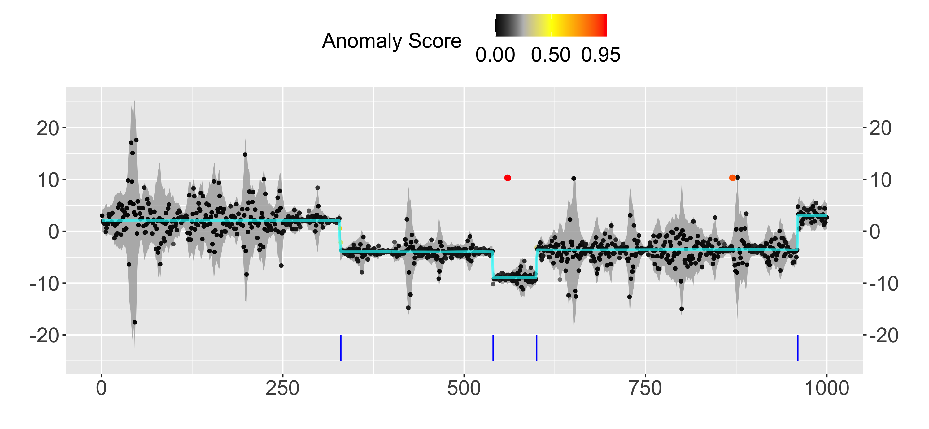
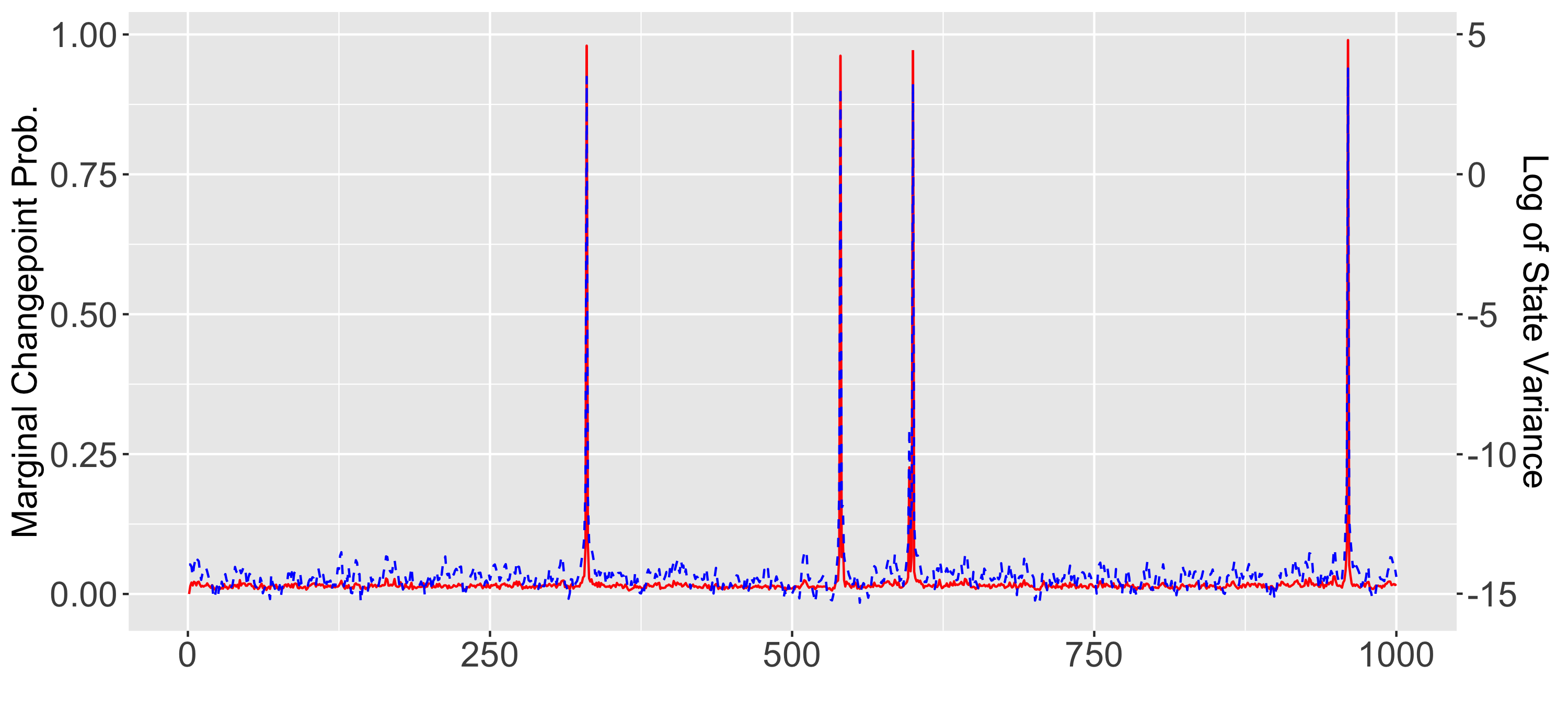
Figure 1: Example Plots for Changes in Mean with Stochastic Volatility

The top plot shows an example of simulated data with two added outliers (colored in red and orange). The anomaly scoring shows local adaptive of the algorithm; the first (left) outlier (above a low volatility region) has the highest score while the second (right) outlier (above a high volatility region) has a lower score. The cyan lines indicate posterior mean of $\{\beta_{t}\}$; vertical blue lines indicate predicted changepoints and gray bands indicate $95\%$ point-wise credible bands for the data excluding the anomaly process component. The bottom plot shows the marginal probability of being a changepoint at each time step (red line) and $\{\log(\omega_{t-D}^{2})\}$ (blue dashed line); the marginal probability at each time step $t$ is calculated from the percentage of posterior simulations of $\log(\omega_{t-D}^{2})$ that exceed the changepoint threshold $\gamma$. We can see, as a result of the threshold variable, $\{\log(\omega_{t-D}^{2})\}$ spikes when changepoint is predicted and comes down right-away; this is key for not over-predicting in regions of high-volatility.

Table 1: Mean Changes with Stochastic Volatility

Algorithms	Rand Avg.	Adj. Rand Avg.	F1-Score	Avg. Dist. to True
ABCO	$\textbf{0.95}_{(0.01)}$	$\textbf{0.90}_{(0.02)}$	0.84	$\textbf{0.59}_{(0.14)}$
Horseshoe	$0.63_{(0.02)}$	$0.32_{(0.02)}$	$0.15$	$87.62_{(9.81)}$
R-FPOP	$0.93_{(0.01)}$	$0.86_{(0.02)}$	$0.78$	$6.01_{(2.30)}$
E.Divisive	$0.85_{(0.01)}$	$0.66_{(0.02)}$	$0.58$	$35.07_{(5.74)}$
H-SMUCE	$\textbf{0.95}_{(0.01)}$	$\textbf{0.90}_{(0.02)}$	$0.76$	$16.34_{(4.54)}$

Table details comparisons between ABCO, the horseshoe approach, R-FPOP, E.Divisive and H-SMUCE on simulated data with stochastic volatility. The standard errors for the metrics are shown in subscript parentheses.

Table 1 details results comparing the performance of ABCO with the competing methods. As seen, ABCO performs the best among the competing models, highlighting its robustness to heteroskedastic noise. ABCO and H-SMUCE both achieve the highest average Rand value of 0.95 and the average highest adjusted Rand average of 0.90, with standard errors of 0.01 and 0.02, respectively. This is expected as H-SMUCE is designed to work under heteroskedastic noise. ABCO achieves a better F1-score of 0.84, in comparison to 0.76 of H-SMUCE, showing a better trade-off in terms of precision and recall for ABCO. R-FPOP achieves the second highest F1-score of 0.78 but has a lower average adjusted Rand value of 0.84.

A further statistic to highlight is the average distance from a predicted changepoint to a true changepoint. ABCO has an impressive distance of 0.59 (se 0.14), with almost every predicted changepoint very close to a true changepoint. While R-FPOP and H-SMUCE were similar in terms of other metrics, they feature much greater prediction-to-true distances of 16.01 and 16.34 respectively. This implies that ABCO is more accurate at predicting the correct location and less susceptible to predicting false positives. The ability to avoid false positives in this setting makes ABCO well suited for diverse applications. In comparison, the static Horseshoe algorithm is less accurate in predicting the correct number of changepoints and tends to miss some more subtle change as illustrated by low F1-score of 0.15. This further supports the previous finding in Kowal et al. (2019) that the SV(1) model provides better estimation of the true mean, which in this case was piecewise constant.

Furthermore, within the Bayesian framework, ABCO provides estimates both the local mean and point-wise credible bands. This allows tracking both a constant or varying signal within each cluster. We can see in Figure 1 that the credible bands are able to adapt well to regions of high volatility.

Table 2: Mean Changes with Outliers

Algorithms	Rand Avg.	Adj. Rand Avg.	F1-Score	Avg. Dist. to True
ABCO	$\textbf{0.94}_{(0.02)}$	$\textbf{0.89}_{(0.03)}$	0.76	$1.56_{(0.23)}$
Horseshoe	$0.67_{(0.01)}$	$0.36_{(0.01)}$	$0.07$	$60.25_{(1.67)}$
E.Divisive	$0.79_{(0.01)}$	$0.59_{(0.02)}$	$0.40$	$22.52_{(1.33)}$
R-FPOP	$0.85_{(0.02)}$	$0.65_{(0.05)}$	$0.73$	$\boldsymbol{0.42}_{(0.09)}$
H-SMUCE	$0.91_{(0.01)}$	$0.83_{(0.01)}$	$0.57$	$5.15_{(0.77)}$

Result for ABCO against other changepoint algorithms on simulated data with changes in mean and significant outliers. The metrics mostly match those detailed in Table 1.

3.2 Detecting Changes in the Presence of Outliers

Next we illustrate the effectiveness of ABCO in the presence of significant outliers. 100 time series are generated of length 300, with a single changepoint in mean randomly selected in the middle 50 percent of the series, partitioning the series into two segments. The first segment has a mean of 0 and the second segment has a mean of 2. Both segments have noise simulated by a normal distribution with mean 0 and variance 1. Additionally, for each segment, 5 significant outliers are generated uniformly at random to be 20-30 standard deviations away from the mean. The outliers are chosen to be significantly greater than the change in mean to test robustness against extreme values. We again fit the ABCO model, the static horseshoe model, E.Divisive, R-FPOP and H-SMUCE on the simulated data sets.

Figure 2: ABCO Outlier Scoring / Stochastic Volatility

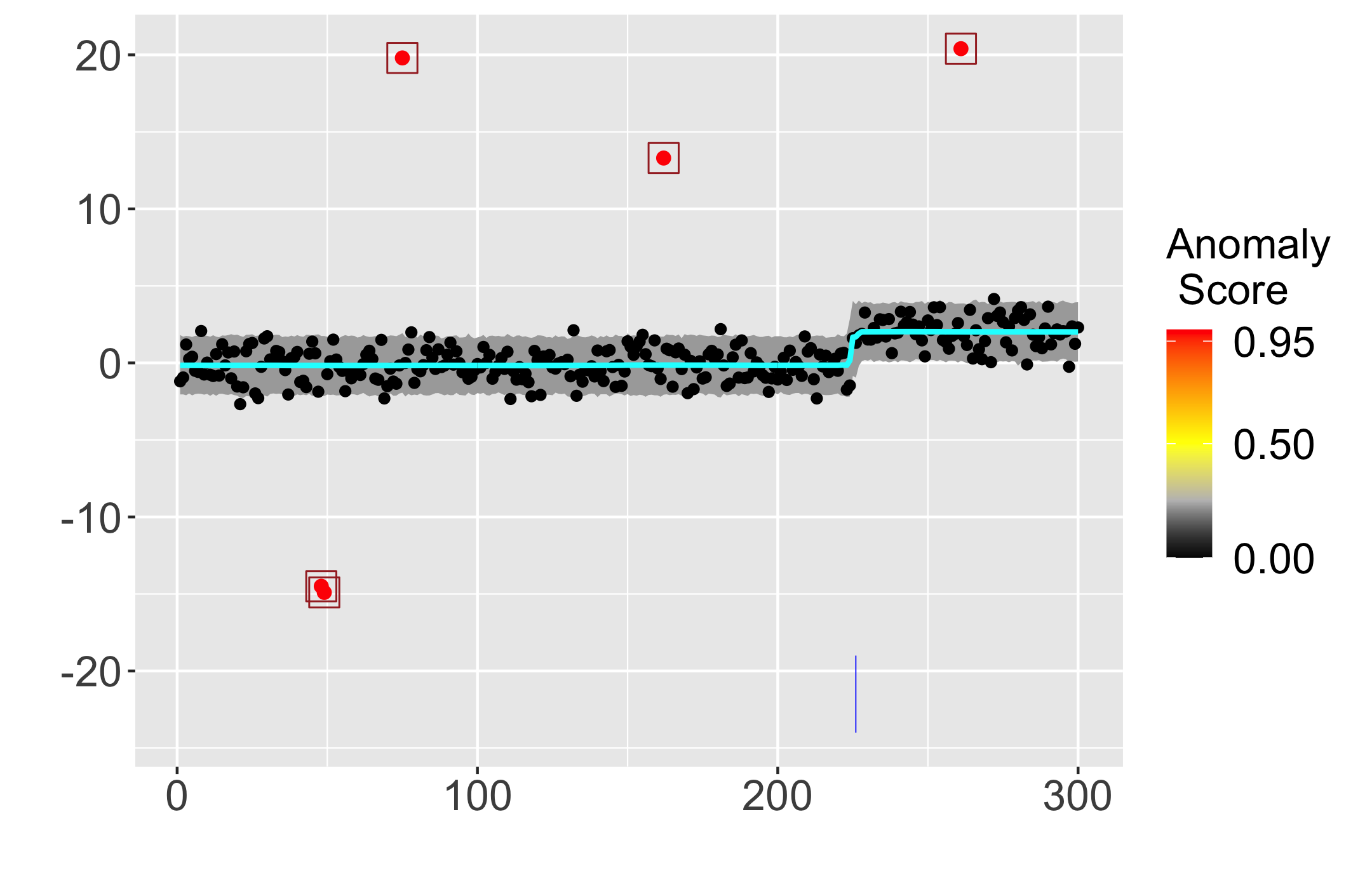
a)	c)
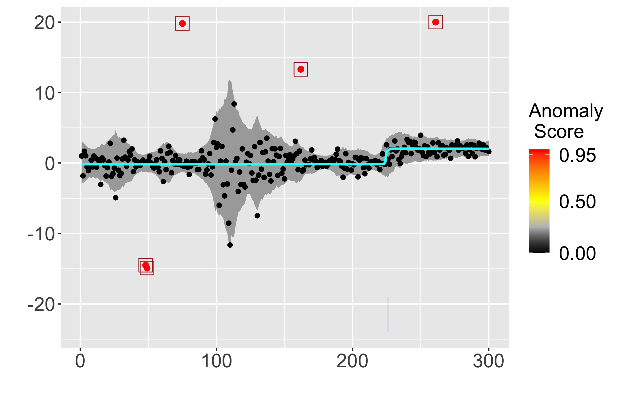
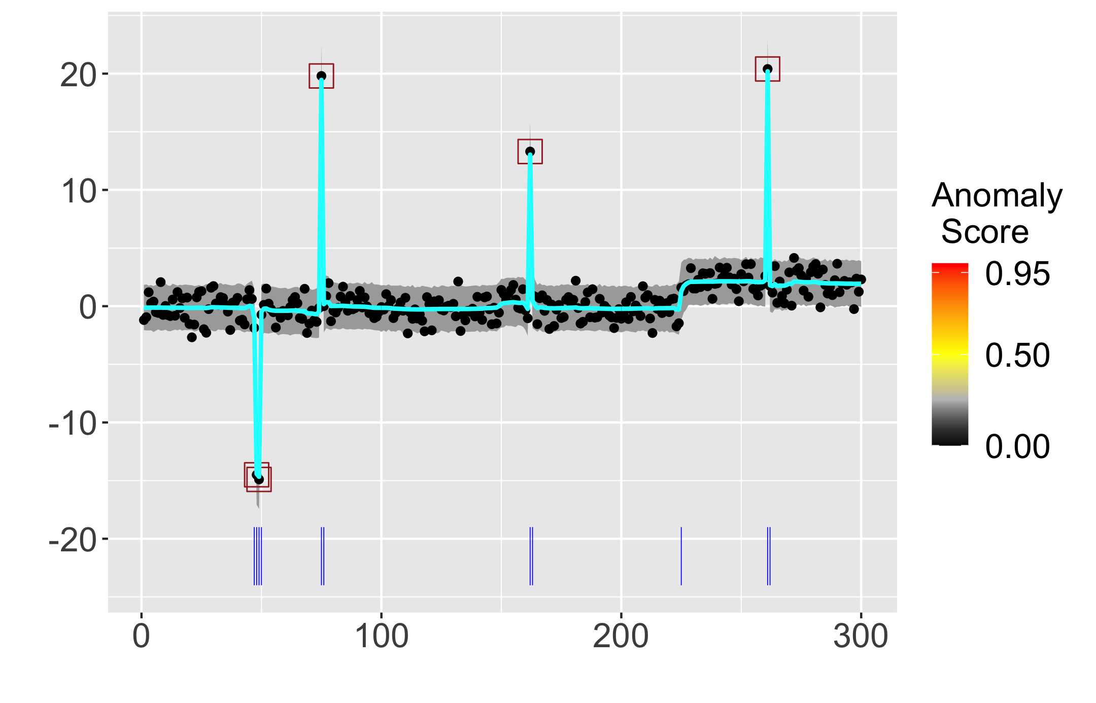
b)	d)

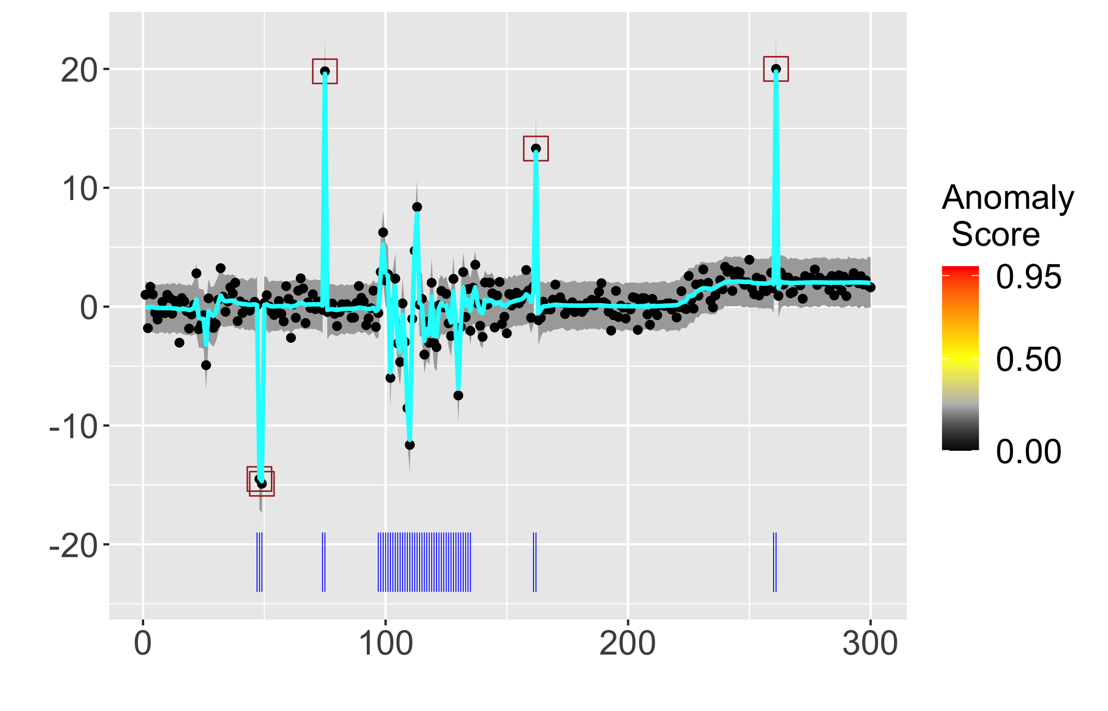
This figure illustrates data generated with same signal and outlier but different noise processes. a) Results of ABCO on data generated with constant noise. b) Results of ABCO without the stochastic volatility component and without the anomaly component on same data as plot a. c) Results of ABCO on data generated with stochastic volatility. d) Results of ABCO without the stochastic volatility component and without the anomaly component on same data as plot c. As seen, ABCO struggles to adapt to these series without both the outlier and the stochastic volatility components included. True positive outliers flagged by the model are outlined by squares. The estimated mean (trend) is shown in cyan; estimated changepoint locations are indicated by blue vertical lines below the series, and credible bands for the observations excluding the estimated outlier process is shown in gray.

The result from the simulation scenario is summarized in Table 2, where ABCO outperforms other models. ABCO achieves highest average Rand value of 0.94 (se 0.02) and highest average adjusted Rand value around 0.89 (se 0.03). H-SMUCE came second with average adjusted rand of 0.83 (se 0.01), while all other algorithms performed quite a bit worse. The key difference between ABCO and H-SMUCE in that ABCO is more accurate at identifying the correct changepoint locations; this is reflected by an average distance from predicted to true changepoints of 1.56 for ABCO in comparison to 5.15 for H-SMUCE. As a result, ABCO has a much higher F1-Score than H-SMUCE. R-FPOP, an algorithm designed to work in presence of outliers, performed similarly to ABCO in terms of F1-score and achieved the best average distance from predicted to true changepoints of 0.42. However, R-FPOP sometimes will under-predict number of changepoints, leading to a much lower average adjusted Rand average. Similar to results from Subsection 3.1, the static horseshoe prior significantly under-performs the dynamic prior of ABCO.

As seen, ABCO works well in both settings of stochastic volatility and significant outliers. This is due to the fact we have decomposed the noise into two components: outlier and heteroskedastic noise. Figure 2 shows an example how these components work together to make ABCO effective. As shown, removing one of the component would lead to over-prediction and decrease in performance of the model. Modeling stochastic volatility within ABCO increases its effectiveness for heterogeneous series while maintaining the same level of performance for series with constant variance. Hence, we recommend including both outlier and heteroskedastic noise when deploying ABCO, in general.

3.3 Linear Trends / Outlier Scoring

Results from Section 3.1 and Section 3.2 have shown ABCO to perform comparably well in comparison to competing methods in settings of changes in mean with outliers or stochastic volatility. One additionally advantage of ABCO is the flexible framework which allow it to detect higher-order changes and flag outliers. For this set of simulations, we will showcase both of these abilities of ABCO by simulating data with changes in linear trend and significant outliers.

Series are generated with a length of 300 with a changepoint randomly selected in the middle 20% of the data. The linear ‘meet-up’ model is utilized to generate the data, meaning the segments are set to be continuous (end of segment 1 becomes the start of segment 2). The start and end of segment 1 as well as end of segment two are uniformly randomly generated between -100 and 100. The segments are set to have a minimum slope difference of 1.5 to ensure separability. Three types of outlier settings are generated: small (5-10 std. dev. away from the true mean), large (25-30 std. dev. away from the true mean) and mixed (5-30 std. dev. away from the true mean). We generate N = 100 series for each outlier setting, with 5-10 outliers randomly generated for each segment. Since none of the other competing methods work well for linear trends, we ran ABCO in each of the three settings and reported the results terms of both changepoint detection accuracy and outlier detection accuracy.

Table 3: Outlier Extension: Linear Trend Results for ABCO

Outlier Type	Rand Avg.	Adj. Rand Avg.	True Positive Rate	False Positive Rate
Small	$0.95_{(0.01)}$	$0.91_{(0.03)}$	$0.71_{(0.04)}$	$0.001_{(0.0001)}$
Large	$0.95_{(0.02)}$	$0.90_{(0.03)}$	$0.95_{(0.02)}$	$0.001_{(0.0005)}$
Mixed	$0.94_{(0.02)}$	$0.88_{(0.03)}$	$0.92_{(0.02)}$	$0.001_{(0.0002)}$

Result for ABCO on predicting both changepoints and outliers in linear settings. Average Rand and adjusted Rand reflect accuracy of changepoint detection, while true positive and false positive rates measures accuracy of outlier detection. The standard error for all measurement are shown in parentheses.

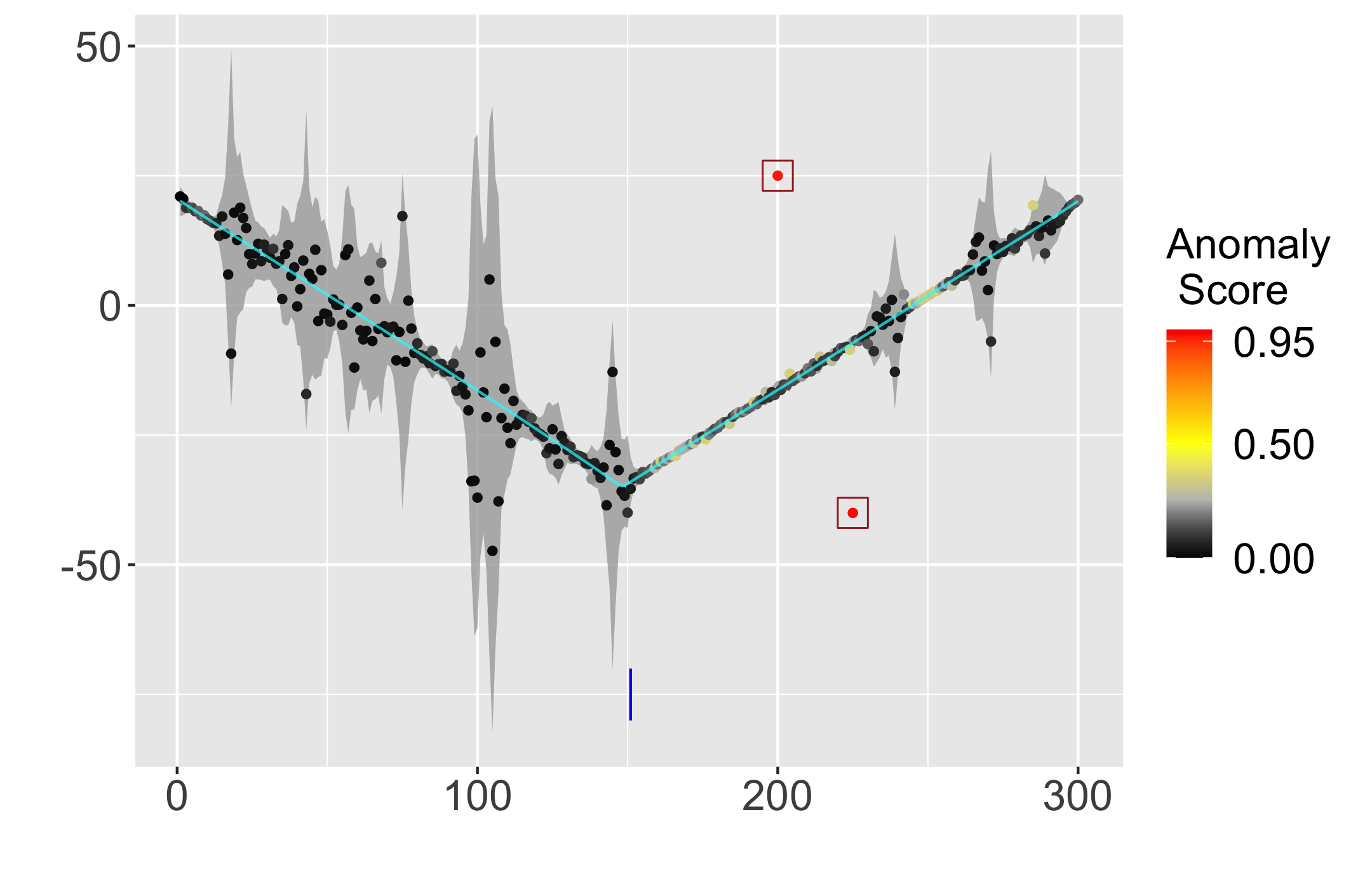
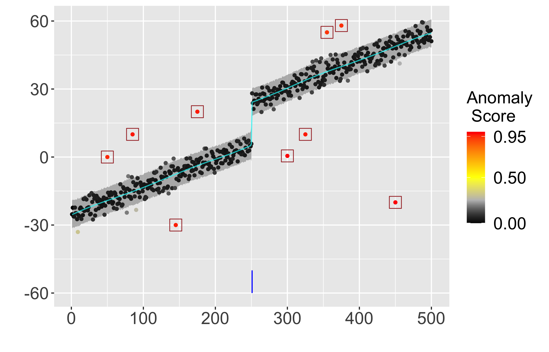
Figure 3: Linear Data Examples

Examples of plots generated using simulated series with linear trends, changepoints and outliers. Left figure shows an example of a linear meet-up model generated with stochastic volatility and 2 outliers. Right figure shows a common linear trend with a jump and several outliers. Outlier scoring is calculated by the ABCO model with true positive outliers outlined by squares. Vertical lines below the series indicate estimated changepoint locations; cyan line denote the estimated mean (trend) with 95% credible bands for the estimated signal plus noise (excluding the estimated outlier component) in gray.

For ABCO, outliers are flagged using the outlier scoring detailed in Section 2.2. We choose a cutoff threshold $0.95$ for $\{o_{t}\}$. Both true positive rate and false negative rate for outliers are reported in Table 3. As seen, ABCO is able to have a high true positive rate and a low false positive rate for all three types of outliers (an example of outlier scoring is seen in Figure 3). At the same-time, ABCO is able to maintain an average adjusted Rand value of at least 0.88, signaling its effectiveness in identifying true changepoints. The detection of both changepoints and outliers simultaneously allows ABCO to provide more information for analysis. As we can see in Figure 3, a series may contain a significant amount of outliers, a very difficult or impossible setting for other changepoint algorithms. The ability to incorporate both heteroskedastic noise and outlier detection makes ABCO very widely applicable. More simulation scenarios for ABCO including varying signal-to-noise ratios, changing variance and dynamic regression analysis are shown in the Online Appendix.

4 Illustrative Applications

4.1 Gross Domestic Product Growth Rate

For the first application we examine changepoints in gross domestic product (GDP) growth rate across three countries (United States, Japan and France). Gross domestic product measures total value of goods/services produced by an economy and represents a key indicator for the country’s economic status (Landefeld, 2000). Understanding changes in long-term pattern of GDP growth rate can provide important information about economic transitions (Antolin-Diaz et al., 2017) and highlight difference between the present versus the past. We chose United States, Japan and France as they are three first world countries in different regions of the world. For the United States, we utilize yearly data from 1940 to 2021. For Japan and France, due to data availability, we utilize yearly data from 1961 to 2021.

Figure 4: GDP Growth Rate Results

United States	Japan
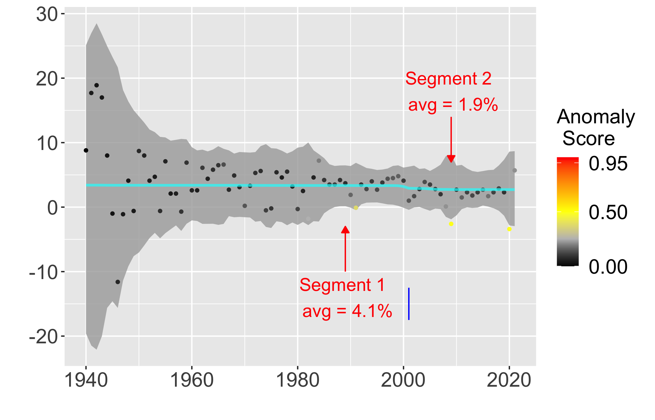
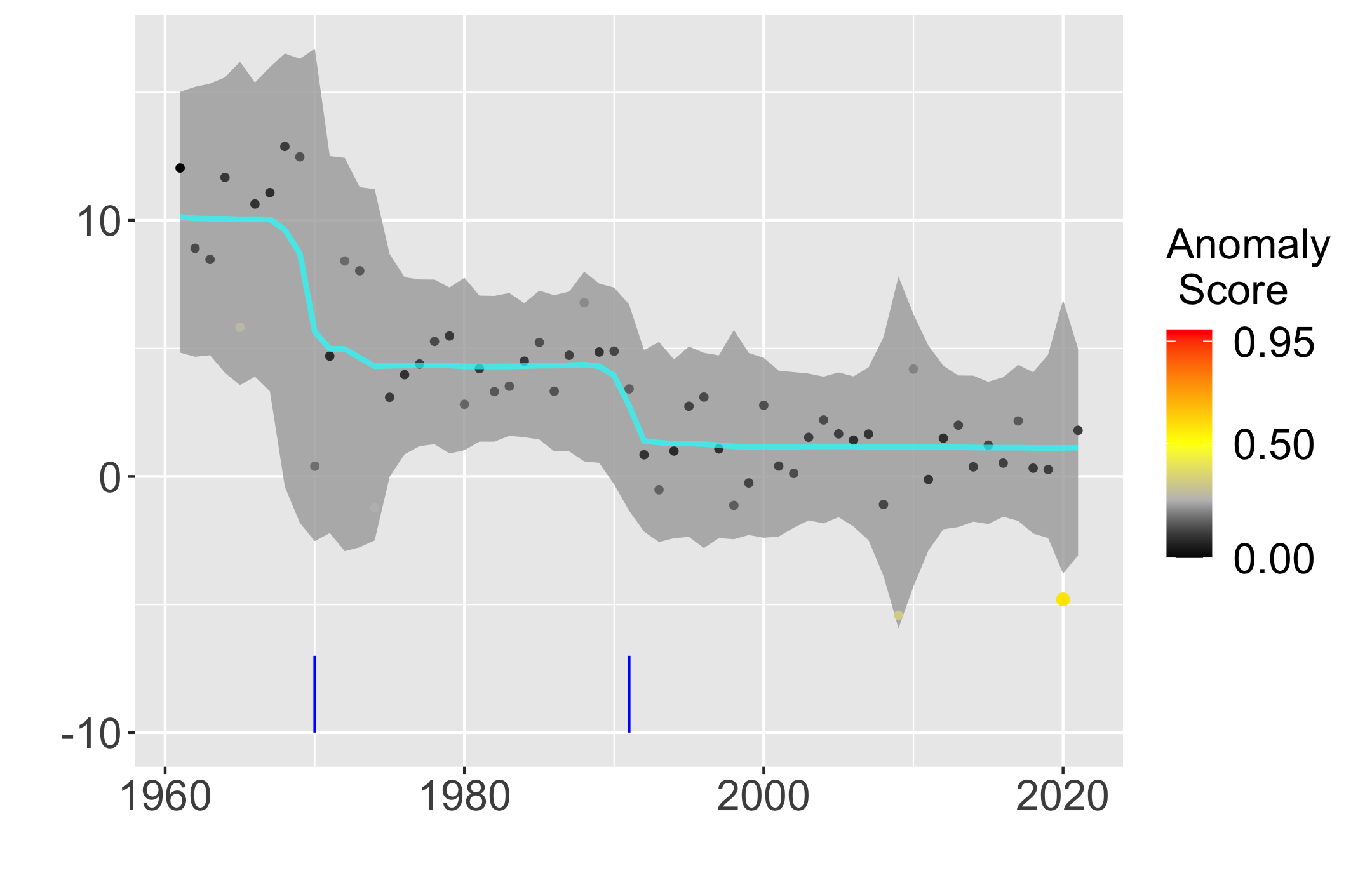
France

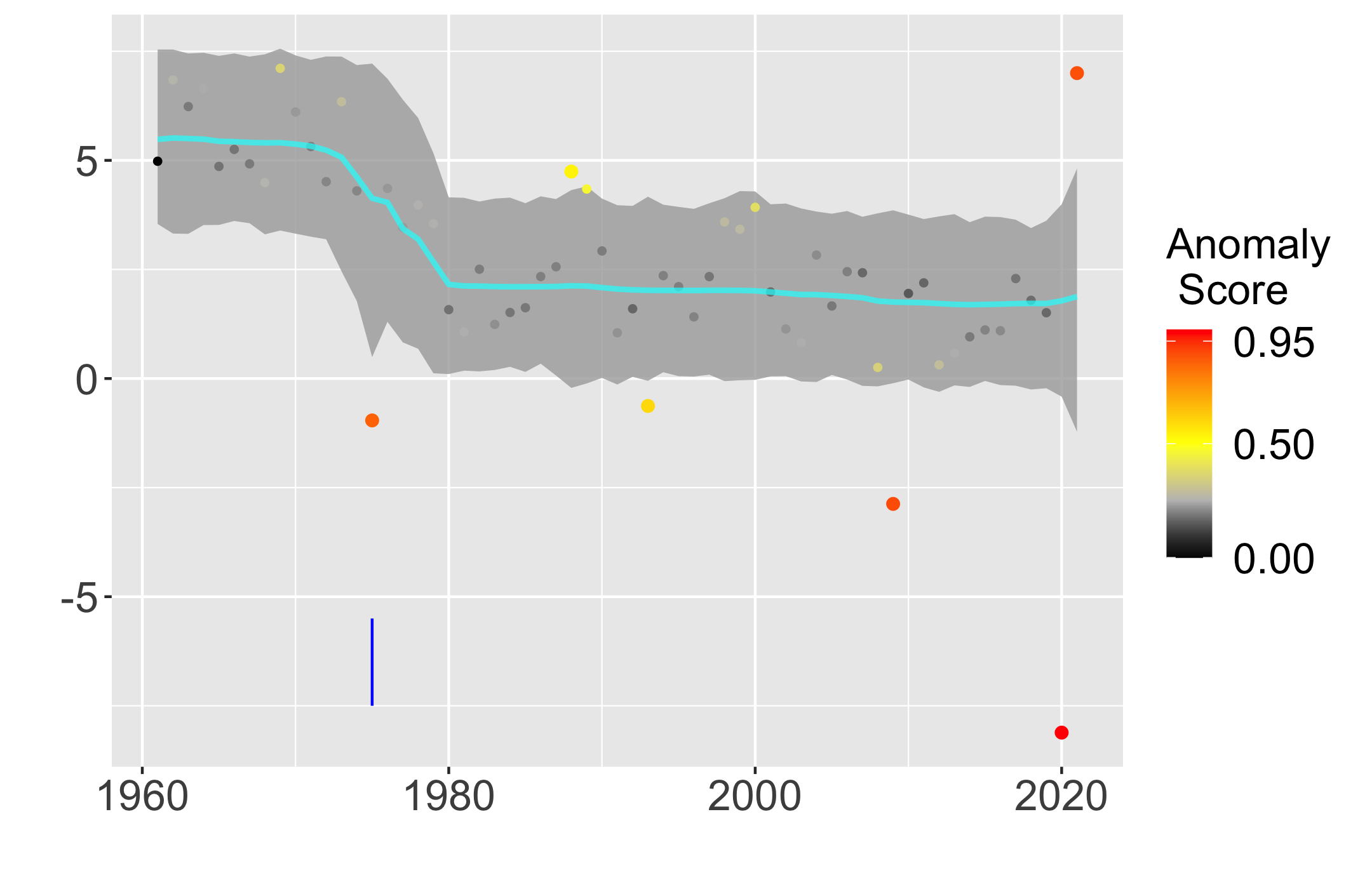
Figure illustrates results of ABCO on GDP growth rate in the United States, Japan and France. The posterior mean predicted trend are shown in cyan and 95% credible band for signal plus noise is shown in light gray. Points are colored according to anomaly scores and estimated changepoints are given by the blue vertical bar.

Figure 4 illustrates results ABCO on the three series. As seen, two features of the series make changepoint detection difficult. First, the series exhibit heteroskedastic variance with regions of high/low variability. For example, in the United States, the GDP growth varied significantly more from 1940-1960 in comparison to from 2000-2020. Second, the series contain significant outliers as a result of economic crashes and boosts. These outliers can potentially lead to over-prediction for changepoint algorithms.

ABCO is able to account for these features and predict reasonable changepoints for each of the three series. For the United States, ABCO predicts one changepoint in the year 2001 after the dot-com crash. This changepoint makes sense as a slowdown in the United States economy since the 2000 has been previously documented (Antolin-Diaz et al., 2017; Cardarelli & Lusinyan, 2015). Looking at historical data, the average GDP growth for the United States between 1940 to 2000 was 4.1$\%$; in comparison, the average GDP growth between 2001-2021 was $1.9\%$. This change represents a significant shift for the US economy. Another feature to highlight is that ABCO adjusts well to the high volatility from the 1940-1950. Despite the fact there exist a small shift in the trend during that time period, ABCO does not predict a changepoint due to high uncertainty at the time period.

For Japan, ABCO predicts two changepoints during the year 1970 and 1991. The underlying trend predicted by ABCO shows a significant slowdown of the Japanese economy over the last 60 years. Looking at the data, the average GDP growth rate in Japan from 1960-1969 was $10.4\%$, from 1970-1990 was $4.3\%$ and from 1990-2021 was $0.8\%$. The changepoints support previous findings in literature that the Japanese economy growth has significantly decreased in the last 3 decades due to their aging workforce (Fukao et al., 2021). For France, ABCO predicts one changepoint around the year 1974 and relatively stable GDP growth of around $1.9\%$ a year for the last 40 years. The results from the French economy shows ABCO’s robustness to outliers. As seen, there exist 3 significant outliers in the years 2008, 2020 and 2021 from the housing crash and the Covid pandemic. As seen, ABCO accounts for these outliers and flags them with high outlier score without letting them affect the underlying trend.

4.2 US Total Imports/Exports

Figure 5: US Imports/Exports Results

Imports Data	Exports Data
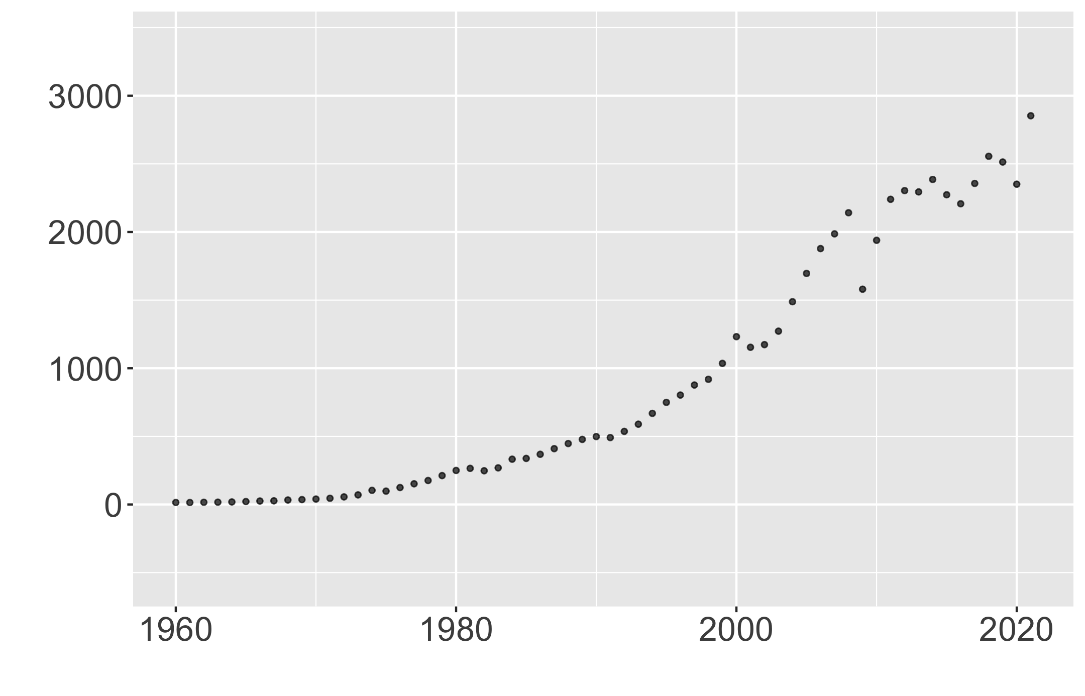
Imports Results	Exports Results

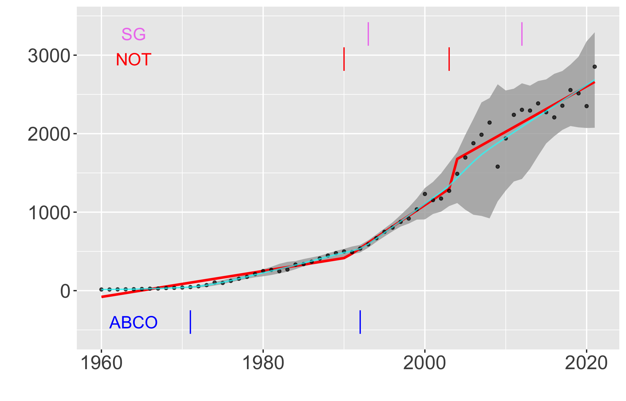
Top plots show the data across last 60 years for yearly imports and exports in units of billions of dollars. Bottom plots show changepoints predicted by ABCO, NOT and Strucchange in blue, red and violet respectively. The posterior mean resulting from ABCO is shown in cyan with $95\%$ credible bands for signal plus noise shown in light gray. The resulting lines of best fit from segmentation predicted by NOT is shown in red.

For the next application, we examine ABCO’s capability to detect changes in linear trend by looking at the United States yearly total import and export across the last 60 years. We chose to examine imports and exports series as they are two important economic indicators and show clear linear trends. However, two features of the series still make changepoint detection difficult. First, the changes in slope appear very subtle, making it challenging to pinpoint the exact changepoint location. Second, the series shows increased volatility over time, especially across the last 20 years. We compare ABCO against two linear changepoint algorithms: narrowest over threshold (NOT, Baranowski et al., 2019) and strucchange (SG, Zeileis et al., 2002). NOT is a non-parametric method that utilizes a series of generalized likelihood ratio test to produce the best segmentations. Strucchange utilizes a generalized fluctuation framework along with F-tests to identify optimal segmentations. The methods are implemented through R packages not and struccchange.

Figure 5 illustrates the results of the three methods on the series. For imports, ABCO predicts two changepoints in years 1971 and 1992. For exports, ABCO predicts two changepoints in years 1971 and 1986. The changepoint at 1971 for both imports and exports are missed by the competing methods as it’s a subtle change in a low volatility area. As seen, this changepoint is well-supported in the data as its clear that the imports/exports began to increase linearly as a faster rate since the 1970. Additionally, 1970 also marks the year where US began running trade deficits (Reinbold & Wen, 2019), showing further evidence for the changepoint. For the other changepoint in both series, NOT also predicts a changepoint in the year 1986 for exports and a changepoint close to 1992 for imports. However, both NOT and Strucchange predicts changepoints after the 2000s, in regions of high volatility. ABCO does not predict those changepoints but rather accounts for increased uncertainty with the adaptive variance.

To further compare the changepoints predicted by the algorithms, we fit a simple linear regression model for each resulting segmentation and compare the Akaike information criterion (AIC) of the resulting fit. The resulting linear best fits from NOT are also shown in Figure 5 in red lines. For imports, ABCO produced an AIC of 618.79, in comparison to 706.47 from NOT and 729.11 from Strucchange. For exports, ABCO produced an AIC of 619.95, in comparison to 634.44 from NOT and 700.49 from Strucchange. These results illustrate that ABCO produces the best segmentation for the underlying series, further highlighting ABCO’s effectiveness in heteroskedastic series.

4.3 Policy Change on Smoking in Italy

For an illustration of applying ABCO to an interrupted time series, we consider the effect of a smoking ban in Sicily, Italy on the hospital admission rate for acute coronary events (ACE) (Barone-Adesi et al., 2011). Monthly ACE rate is recorded from 2002 to 2006 with a smoking ban taking place January of 2005. The dataset has been previously analyzed using interrupted time series in Bernal et al. (2017). The series is shown in Figure 6, with the results of applying the modified ABCO method. The most prominent feature is a major level shift in the underlying trend after the smoking ban in January of 2005, but the slope (rate of increase over time) before and after the intervention appears very similar.

Figure 6: Effect of Smoking Ban on Rate of Acute Coronary Events in Sicily, Italy

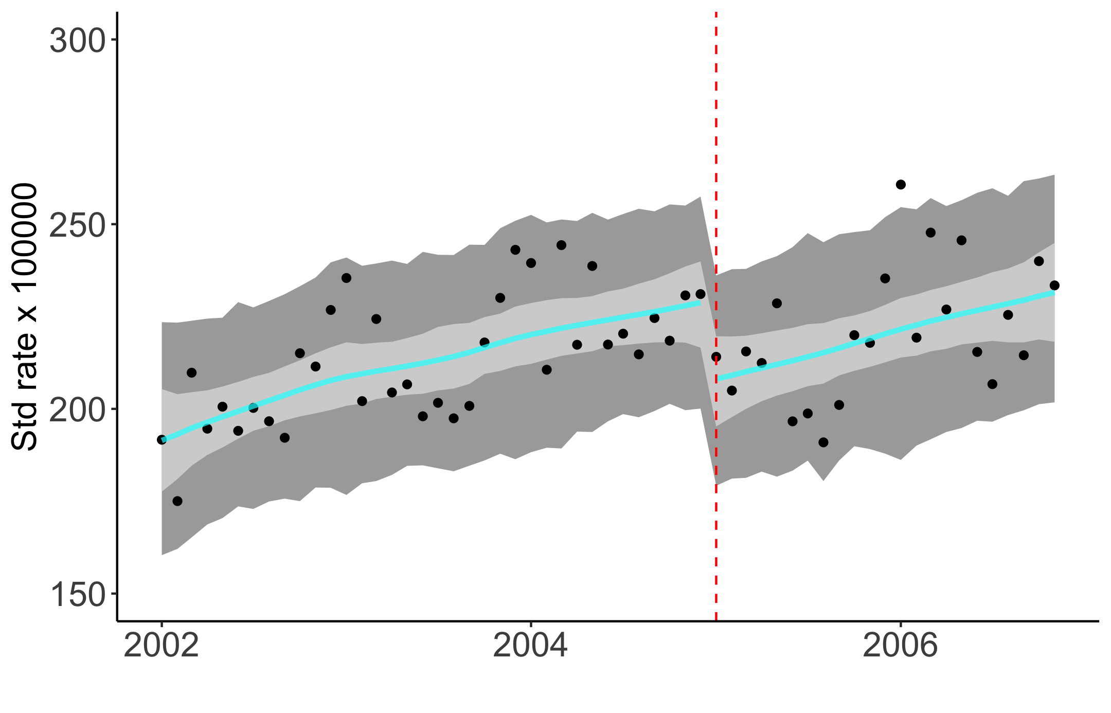
a)	c)
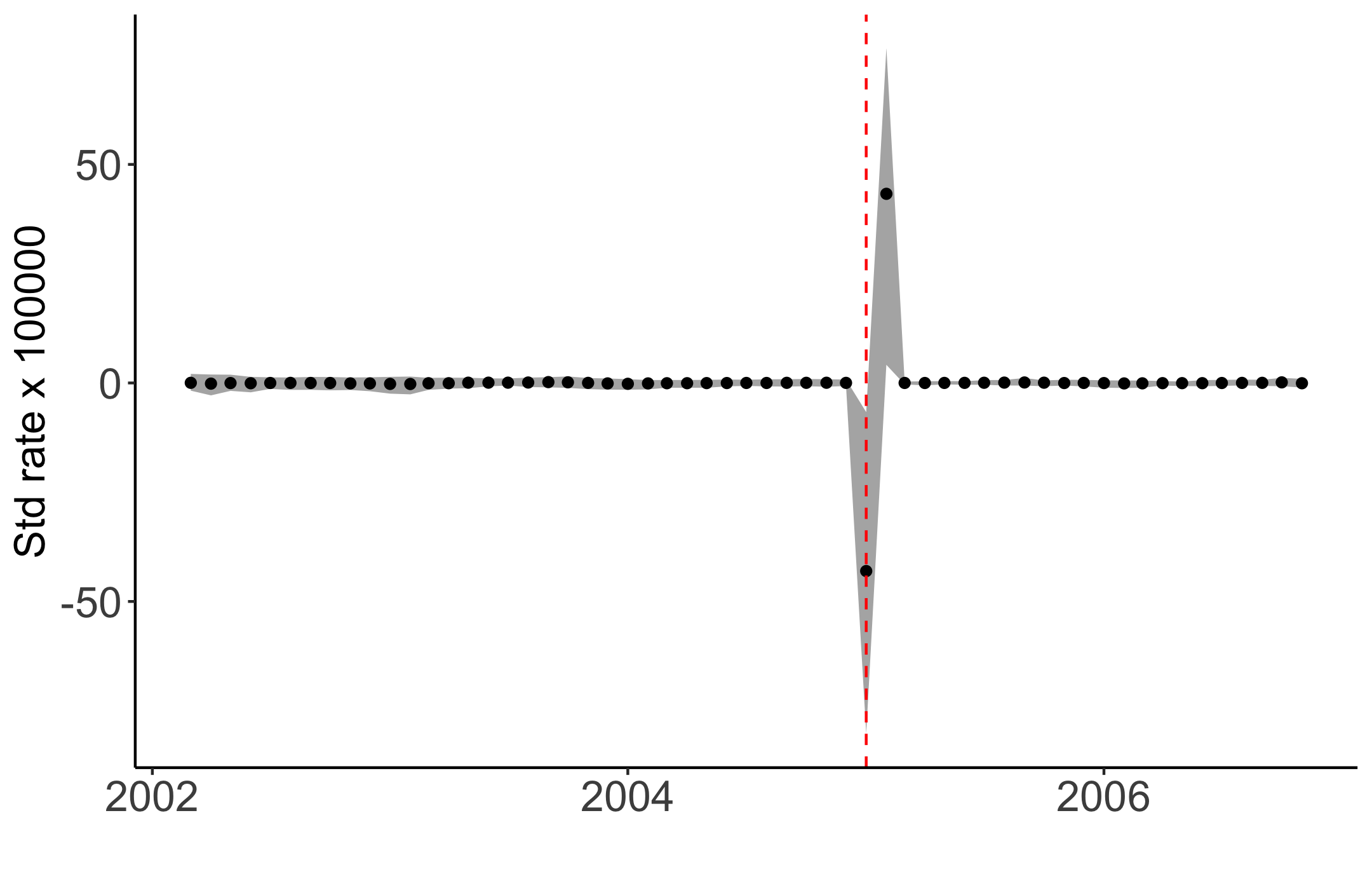
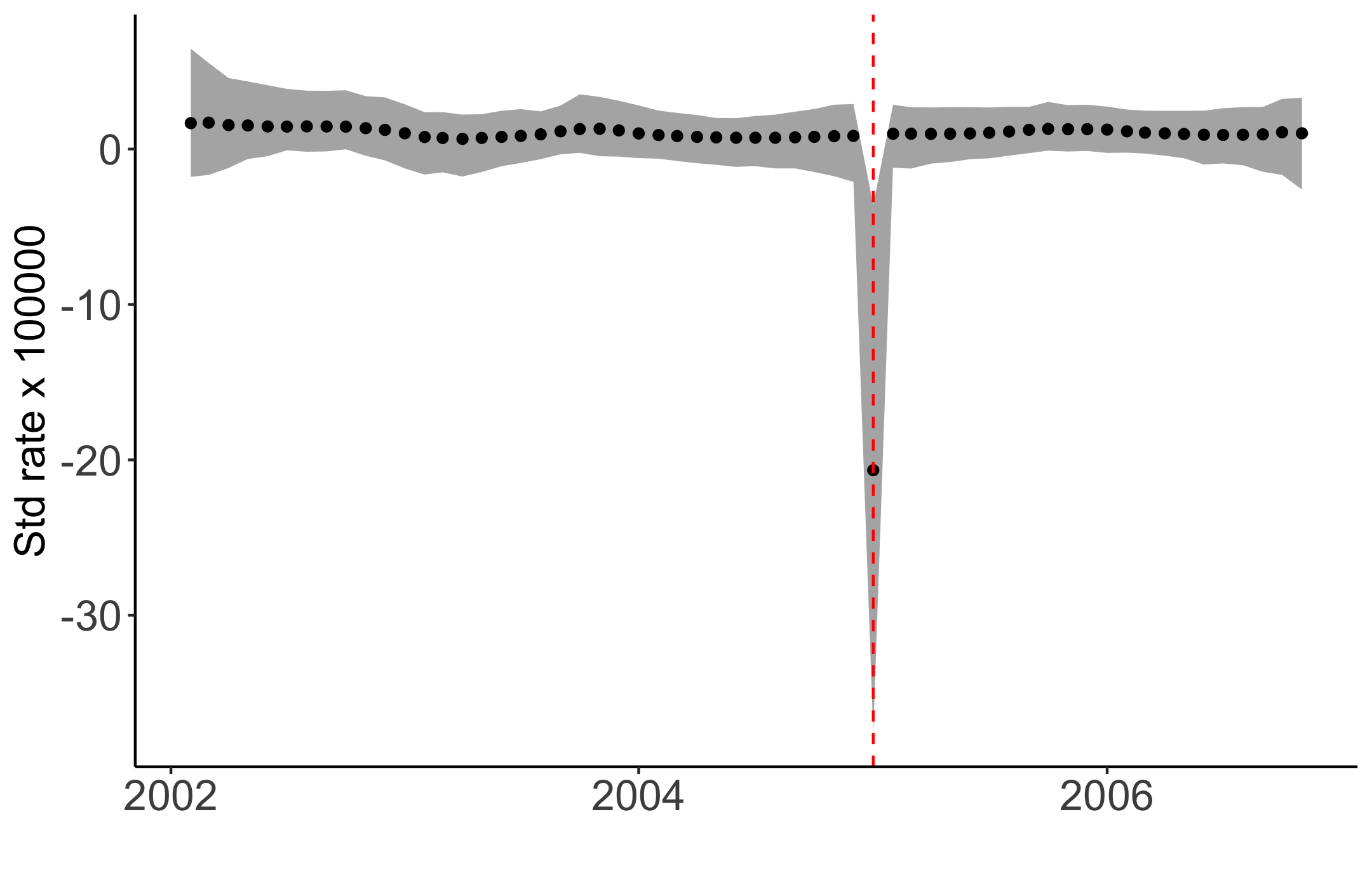
b)	d)

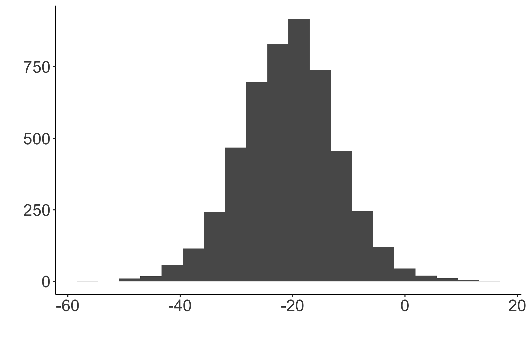
a) ABCO for interrupted time series results: the plot shows the standardized rate of ACE over time. The posterior mean trend for $\{\beta_{t}\}$ is shown in cyan along with 95$\%$ credible bands for $\{\beta_{t}\}$ in light gray and 95$\%$ credible bands for $\{y_{t}\}$ in dark gray. The estimated trend appears to be linear before and after the intervention data, with a level shift downward, but with little change in slope. b) First difference in trend: the plot shows the first degree difference in the trend $\{\bigtriangleup\beta_{t}\}$ from the modified ABCO $(\{\bigtriangleup^{2}\!\beta_{t}=\omega_{t}+\upsilon_{t}\})$ along with 95$\%$ credible bands in dark gray. With the single departure from the otherwise constant increments we have no evidence of anticipatory or temporary intervention effects; the intervention appears to have only had an immediate, but sustained impact, in intercept in this case. c) Second difference in trend: the plot shows the second degree difference in the trend $\{\bigtriangleup\beta_{t}\}$ from the modified ABCO along with 95$\%$ credible bands in dark gray. The negative departure at time $\pi$ and the positive bounce-back of similar magnitude at time $\pi+1$ further support the claim of a shift in intercept but not in slope at time of intervention. d) Posterior distribution at the time of intervention: the plot shows the density of the posterior distribution of the first difference of $\{\beta_{t}\}$ at the intervention time $\pi$ (i.e. $\bigtriangleup\beta_{\pi}$). From here the modified ABCO approach allows model-based inference on the effect size at intervention.

Our overall conclusions in this case are very similar to the finding of traditional interrupted time series analysis (Bernal et al., 2017). Some of the advantages the modified ABCO provides is flexibility in estimating the trends pre- and post-intervention; robustness to any outliers or heteroskedastic noise; adaptive uncertainty quantification over time and at the intervention time in particular. We note from the figure that there is roughly constant variability in changes in the trend (although slightly larger post intervention) except at time $\pi$ where ABCO has estimated substantially more uncertainty about the intervention effect size. This is highlighted in the right panel which shows the estimated posterior distribution for $\bigtriangleup\beta_{\pi}$ which is centered around -20, but with substantial variability. Additional standard model checking was performed but not shown.

5 Conclusion

We have proposed an adaptive Bayesian changepoint model with the ability to detect multiple changepoints within a time series. The model separates the series at each time-step into a trend component, an outlier component and a noise component. For trend estimation with breaks, a horseshoe-like shrinkage is placed on the $Dth$ difference of the trend component through a threshold stochastic volatility model with $Z$-distributed innovations. This shrinkage ensures most increments are relatively small or even nearly zero while allowing some isolated changes to be significantly large. The threshold variable is used to classify large changes as changepoints. For the outlier component, a horseshoe-plus prior is utilized to model extreme values in the data. For the noise component, a stochastic volatility model is specified to adapt both change and outlier detection to regions of both high and low volatility, whether stochastic or not. Together, all three components allow great flexible adaptive trend modeling, changepoint detection, and outlier scoring.

Through simulation experiments and illustrative applications we have highlighted the unique strengths of ABCO and shown settings were it outperform competing methods, i.e. changepoint series with significant outliers and/or non-constant variance. With a Bayesian framework, ABCO provides a reliable means for simultaneously estimating changepoints and scoring anomalies, and it can be further extended, as we demonstrated dynamic regression specifications. Further directions include analysis of multivariate series and incorporating covariates into change and outlier detection equations.

SUPPLEMENTARY MATERIAL

Online Appendix:

Appendix contains details about the MCMC sampling procedures, and more simulations comparing effectiveness of ABCO against other changepoint algorithms.

Code:

Zip file containing the code for running ABCO. The zip file includes all sampling algorithms for ABCO and ABCO for interrupted time series. It also includes code for running all simulations and real world examples seen in the paper.

References

- (1)
- Adams & MacKay (2007) Adams, R. P. & MacKay, D. J. (2007), ‘Bayesian online changepoint detection’, arXiv:0710.3742 .
- Antolin-Diaz et al. (2017) Antolin-Diaz, J., Drechsel, T. & Petrella, I. (2017), ‘Tracking the slowdown in long-run gdp growth’, Review of Economics and Statistics 99(2), 343–356.
- Baranowski et al. (2019) Baranowski, R., Chen, Y. & Fryzlewicz, P. (2019), ‘Narrowest‐over‐threshold detection of multiple change points and change‐point‐like features’, Journal of the Royal Statistical Society, Series B 81, 649–672.
- Barone-Adesi et al. (2011) Barone-Adesi, F., Gasparrini, A., Vizzini, L., Merletti, F. & Richiardi, L. (2011), ‘Effects of italian smoking regulation on rates of hospital admission for acute coronary events: a country-wide study’, PLoS One 6.
- Bernal et al. (2017) Bernal, J. L., Cummins, S. & Gasparrini, A. (2017), ‘Interrupted time series regression for the evaluation of public health interventions: a tutorial’, International Journal of Epidemiology 46, 348–355.
- Bhadra et al. (2017) Bhadra, A., Datta, J., Polson, N. G. & Willard, B. (2017), ‘The horseshoe+ estimator of ultra-sparse signals’, Bayesian Analysis 12(4), 1105–1131.
- Braun et al. (2000) Braun, J., Braun, R. & Müller, H.-G. (2000), ‘Multiple changepoint fitting via quasilikelihood, with application to dna sequence segmentation’, Biometrika 87, 301–314.
- Cardarelli & Lusinyan (2015) Cardarelli, M. R. & Lusinyan, M. L. (2015), US total factor productivity slowdown: evidence from the US states, International Monetary Fund.
- Carvalho et al. (2009) Carvalho, C. M., Polson, N. G. & Scott, J. G. (2009), ‘Handling sparsity via the horseshoe’, AISTATS 5, 73–80.
- Chen et al. (2019) Chen, G., Lu, G., Shang, W. & Xie, Z. (2019), ‘Automated change-point detection of eeg signals based on structural time-series analysis’, IEEE Access 7.
- Chen & Gupta (1997) Chen, J. & Gupta, A. (1997), ‘Testing and locating variance changepoints with application to stock prices’, Journal of American Statistics Association 92, 739–747.
- Cho & Fryzlewicz (2015) Cho, H. & Fryzlewicz, P. (2015), ‘Multiple-change-point detection for high dimensional time series via sparsified binary segmentation’, J. R. Statist. Soc. B 77, 475–507.
- Ebrahimzadeh et al. (2019) Ebrahimzadeh, Z., Zheng, M., Karakas, S. & Kleinberg, S. (2019), ‘Pyramid recurrent neural networks for multi-scale change-point detection’, ICLR .
- Fearnhead & Rigaill (2017) Fearnhead, P. & Rigaill, G. (2017), ‘Changepoint detection in the presence of outliers’, Journal of American Statistical Association 114, 169–183.
- Fuentes-García et al. (2019) Fuentes-García, R., Mena, R. H. & Walker, S. G. (2019), ‘Modal posterior clustering motivated by hopfield’s network’, Computational Statistics & Data Analysis 137, 92–100.
- Fukao et al. (2021) Fukao, K., Kim, Y. G. & Kwon, H. U. (2021), ‘The causes of japan’s economic slowdown: An analysis based on the japan industrial productivity database’, International Productivity Monitor 40, 56–88.
- García & Gutiérrez-Peña (2019) García, E. C. & Gutiérrez-Peña, E. (2019), ‘Nonparametric product partition models for multiple change-points analysis’, Communications in Statistics-Simulation and Computation 48(7), 1922–1947.
- James & Matteson (2014) James, N. A. & Matteson, D. S. (2014), ‘ecp: An r package for nonparametric multiple change point analysis of multivariate data’, Journal of Statistical Software 62.
- Kim et al. (1998) Kim, S., Shephard, N. & Chib, S. (1998), ‘Stochastic volatility: Likelihood inference and comparison with arch models’, Review of Economic Studies 65, 361–393.
- Ko et al. (2015) Ko, S. I., Chong, T. T. & Ghosh, P. (2015), ‘Dirichlet process hidden markov multiple change-point model’, Bayesian Analysis 10(2), 275–296.
- Kowal et al. (2019) Kowal, D., Matteson, D. & Ruppert, D. (2019), ‘Dynamic shrinkage process’, J. R. Statist. Soc. B 81.
- Landefeld (2000) Landefeld, J. S. (2000), ‘Gdp: One of the great inventions of the 20th century’, Survey of Current Business 80(1), 6–14.
- Liu et al. (2013) Liu, S., Yamada, M., Collier, N. & Sugiyama, M. (2013), ‘Change-point detection in time-series data by relative density-ratio estimation’, Neural Networks 43, 72–83.
- Luong et al. (2012) Luong, T. M., Perduca, V. & Nuel, G. (2012), ‘Hidden markov model applications in change-point analysis’, arXiv preprint arXiv:1212.1778 .
- Maheu & Yang (2016) Maheu, J. M. & Yang, Q. (2016), ‘An infinite hidden markov model for short-term interest rates’, Journal of Empirical Finance 38, 202–220.
- Matteson & James (2014) Matteson, D. S. & James, N. A. (2014), ‘A nonparametric approach for multiple change point analysis of multivariate data’, Journal of the American Statistical Association 109, 334–345.
- Monteiro et al. (2011) Monteiro, J. V., Assunçao, R. M. & Loschi, R. H. (2011), ‘Product partition models with correlated parameters’, Bayesian Analysis 6(4), 691–726.
- Park & Dunson (2010) Park, J.-H. & Dunson, D. B. (2010), ‘Bayesian generalized product partition model’, Statistica Sinica pp. 1203–1226.
- Pein et al. (2017) Pein, F., Sieling, H. & Munk, A. (2017), ‘Heterogeneous change point inference’, Journal of the Royal Statistical Society: Series B (Statistical Methodology) 79(4), 1207–1227.
- Peluso et al. (2019) Peluso, S., Chib, S. & Mira, A. (2019), ‘Semiparametric multivariate and multiple change-point modeling’, Bayesian Analysis 14(3), 727–751.
- Rabiner (1989) Rabiner, L. R. (1989), ‘A tutorial on hidden markov models and selected applications in speech recognition’, Proceedings of the IEEE 77(2), 257–286.
- Rehman et al. (2016) Rehman, M. H. u., Liew, C. S., Abbas, A., Jayaraman, P. P., Wah, T. Y. & Khan, S. U. (2016), ‘Big data reduction methods: A survey’, Data Sci. Eng. 1, 265–284.
- Reinbold & Wen (2019) Reinbold, B. & Wen, Y. (2019), ‘How industrialization shaped america’s trade balance’.
- Saatçi et al. (2010) Saatçi, Y., Turner, R. & Rasmussen, C. E. (2010), ‘Gaussian process change point models’, ICML 10 Proceedings of the 27th International Conference on International Conference on Machine Learning pp. 927–934.
- Serumaga et al. (2011) Serumaga, B., Ross-Degnan, D., Avery, T., Elliott, R., Majumdar, S. R., Zhang, F. & Soumerai, S. (2011), ‘Effect of pay for performance on the management and outcomes on hypertension in the united kingdom: Interrupted time series study’, BMJ 342.
- Solow (1987) Solow, A. (1987), ‘Testing for climate change: An application of the two-phase regression model’, Journal of Climate and Applied Meteorology 26.
- Tan et al. (2015) Tan, B. A., Gerstoft, P., Yardim, C. & Hodgkiss, W. S. (2015), ‘Change-point detection for recursive bayesian geoacoustic inversions’, The Journal of the Acoustical Society of America 137, 1962–1970.
- Wagner et al. (2002) Wagner, A. K., Soumerai, S. B., F., Z. & Ross-Degnan, D. (2002), ‘Segmented regression analysis of interrupted time series studies in medication use research’, Journal of Clinical Pharmacy and Therapeutics 27, 299–309.
- Wyse & Friel (2010) Wyse, J. & Friel, N. (2010), ‘Simulation-based bayesian analysis for multiple changepoints’, arXiv preprint arXiv:1011.2932 .
- Zeileis et al. (2002) Zeileis, A., Leisch, F., Hornik, K. & Kleiber, C. (2002), ‘strucchange: An r package for testing for structural change in linear regression models’, Journal of statistical software 7, 1–38.
- Zhang et al. (2019) Zhang, W., Gilbert, D. & Matteson, D. S. (2019), ‘Abacus: Unsupervised multivariate change detection via bayesian source separation’, Proceedings of the 2019 SIAM International Conference on Data Mining .