The minimally extended Varying Speed of Light (meVSL)

Abstract

Even though there have been various models of the time-varying speed of light (VSL), they remain out of the mainstream because of their possible violation of physics laws built into fundamental physics. In order to be the VSL as a viable theory, it should inherit the success of special relativity including Maxwell equations and thermodynamics at least. For this purpose, we adopt the assumption that the speed of light, $\tilde{c}$, i.e., $\tilde{c}[a]$, varies for the scale factor, $a$. The background FLRW universe can be defined by the constant cosmic time hypersurface using physical quantities such as temperature, density, $\tilde{c}$, etc. It is because they evolve in cosmic time and the homogeneity of the Universe demands that they must equal at the equal cosmic time. The variation of $\tilde{c}$ accompanies the joint variations of all related physical constants in order to satisfy the Lorentz invariance, thermodynamics, Bianchi identity, etc. We dub this VSL model as a “minimally extended VSL (meVSL)”. We derive cosmological observables of meVSL and obtain the constraints on the variation of $\tilde{c}$ by using current cosmological observations. Interestingly, both the cosmological redshift $z$ and all geometrical distances except the luminosity distance of meVSL are the same as those of general relativity. However, the Hubble parameter of meVSL is rescaled as $H(z)=(1+z)^{-b/4}H^{(\text{GR})}(z)$, where $H^{(\text{GR})}(z)$ denotes the Hubble parameter obtained from general relativity. Thus, it might be used as an alternative solution for the tension of the Hubble parameter measurements. In this manuscript, we provide the main effects of the meVSL model on various cosmological observations including BBN, CMB, SZE, BAO, SNe, GWs, H, SL, and $\Delta\alpha$. Compared to previous VSL models, meVSL might provide alternative solutions for various late time problems of the standard $\Lambda$CDM model. This is the main motivation for proposing the meVSL model.

1 Introduction

While Einstein’s both special relativity (SR) and general relativity (GR) have passed many tests so far, none knows for sure that they apply everywhere under all conditions. SR is an inseparable part of quantum field theory which describes the interactions of elementary particles with an almost incredible degree of accuracy. Many different experiments have been tested for SR without finding any violation of Lorentz invariance (LI). It is believed to be locally exact. But the local LI has to be replaced by GR at cosmological scales. Thus, it is meaningless to quibble about whether SR is generally true and testable at cosmological distances and time scales.

SR contains only one parameter, $c$, the speed of light in a vacuum. In Sec. 3, we show that the universal Lorentz covariance, or, equivalently, the single postulate of Minkowski spacetime is good enough to satisfy the SR [1, 2]. Thus, it is possible to make the LI varying speed of light (VSL) model as long as $c$ is locally (almost) constant and changes at cosmological scales. In order to avoid trivial rescaling of units, one must test the simultaneous variation of $c$ and Newton’s gravitational constant $G$ because both $c$ and $G$ enter as the combination $G/c^{4}$ in the Einstein action [3].

As a possible way to explain problematic observational results which are based on GR, the possibility of various VSLs has sometimes been invoked. The very early idea of a VSL was proposed by Einstein by claiming that a shorter wavelength $\lambda$ leads to a lower speed of light by means of $c=\nu\lambda$ with the constant frequency $\nu$. He assumed that a gravitational field makes the clock run slower by $\nu_{1}=\nu_{2}(1+GM/rc^{2})$ [4]. Dicke assumed that both the wavelength and the frequency vary by defining a refractive index $n\equiv c/c_{0}=1+2GM/rc^{2}$ [5]. He considered a cosmology with an alternative description to the cosmological redshift by using a decreasing $c$ with time. The early VSL cosmology has been proposed to explain the horizon problem of the Big Bang model and to provide an alternative method to cosmic inflation [3, 6, 7, 8, 9, 10, 11, 12, 13, 14, 15, 17, 18, 19, 21, 23, 24, 25, 26, 27, 28, 29, 30, 31, 32, 33, 34]. A VSL model which proposed the change of the speed of light only without allowing the variations of other physical constants is called minimal VSL (mVSL). Petit proposed that if one allows the time variation of c, then one should include the joint variations of all related physical constants. These variations should be based on the consistency of all physical equations and measurements of these constants remain consistent with physics laws during the evolution of the Universe. From this consideration, one might be able to obtain a universal gauge relationship and the temporal variation of the parameters which are regarded as constants [11, 27].

$$G =G_{0}a^{-1}\,,\quad m=m_{0}a\,,\quad c=c_{0}a^{\frac{1}{2}}\,,\quad h=h_{0}a^{\frac{3}{2}}\,,\quad e=e_{0}a^{\frac{1}{2}}\,,\quad\mu=\mu_{0}a\,.$$ (1.1)

In spite of the success of standard cosmology based on GR and FLRW metrics, there have been several shortcomings of standard cosmology. Thus, one of the main motivations for the proposal of VSL models is to look for explanations of some unusual properties of the Universe and to prevail over some of the limitations of standard cosmology [35, 36, 37, 38]. Some VSL models also provide a solution to the cosmological constant problem. The dynamics of VSL models have been investigated in both theoretical and empirical aspects [39, 40, 41, 243, 43, 44, 45, 46, 47, 48, 49, 50, 51, 52, 53].

However, it is pointed out that if one proposes a varying $c$, one needs to rewrite the related physics to replace the current system which depends on the assumption of the constant $c$. This is because the LI builds into fundamental physics [54, 55]. Thus, one cannot just alter the constant $c_{0}$ to the time-varying $c$ in one or two arbitrary equations and leave the rest of physics unchanged. Any viable VSL theory has to provide an integrated viable replacement to the entire set of physical equations and consequent effects (kinematical and dynamical) dependent on $c$. The speed of light in Einstein’s relativity is related to both the metric tensor and Maxwell’s equations. The former determines temporal and spatial measurements, as well as the geometry of null geodesics, and the latter determine the paths of light rays in spacetime. The properties of wavelike solutions of Maxwell’s equations are null geodesics and it is determined by the metric tensor. Thus, they are related to each other. Light rays (i.e., the paths of photons or other massless particles in spacetime) are remedies for the geodesic equation. It might include the redefinition of distance measurements, the validity of LI, the modification of Maxwell’s equations, and consistencies with respect to all other physical theories.

For this purpose, one should investigate the observational status of variations of fundamental constants [56]. A dimensionless physical constant is a constant that is a pure number having no units attached to it. Thus, its numerical value is independent of the used system of units. Sometimes, the terminology of the fundamental physical constant is used to refer to universal dimensionless constants like the fine-structure constant $\alpha$. One might restrict the fundamental physical constants to the dimensionless universal physical ones. Thus, one cannot derive them from any other source [57, 58, 59]. However, the universal dimensioned physical constants, such as the speed of light $c$, the gravitational constant $G$, the Planck constant $h$, and the vacuum permittivity $\epsilon_{0}$, also have been referred to as the fundamental physical constants [60]. The physical constant is denoted as the notion of a physical quantity subjected to experimental measurement which is independent of the time or location of the experiment. The constancy of any physical constant is thus verified by the experiment. One cannot derive fundamental physical constants and thus they have to be measured. The current precision measurements of cosmology might be used to constrain any time variation of fundamental constants.

Dirac made the large numbers hypothesis (LNH) by relating ratios of size scales in the Universe to that of force scales [61]. One obtains very large dimensionless numbers from these ratios. From this hypothesis, he interprets that the apparent similarity of these ratios could imply a cosmology with several unusual features. For example, he proposes that the gravitational constant representing the strength of gravity is inversely proportional to the age of the Universe, $G\propto 1/t$. Also, he suggests that physical constants are actually not constant but depend on the age of the Universe. The purpose of a time-varying $G$ cosmology was proposed inspired by a dislike of Einstein’s GR [62]. It is given by $G=\left(c^{3}/M_{\text{U}}\right)t$ to satisfy Einstein’s conclusions, where $M_{\text{U}}$ and $t$ are the mass and the age of the Universe, respectively. There are recent reviews and applications for this in [63, 64]. The constancy of fundamental physical constants is an important foundation of the laws of physics. If one finds any variation of physical constants, then it implies the discovery of an unknown law of physics. This concerns the speed of light, the gravitational constant, the fine structure constant, the proton-to-electron mass ratio, etc. There have been ongoing efforts to improve the accuracies of experiments on the time-dependence of these constants [65, 66, 67, 68, 69]. From this point of view, the known values of physical constants are just accidental ones of the current epoch when they happen to be measured. Time variation of the fine-structure constant, $\alpha$ based on observation of quasars was announced [70] but an observation based on CH molecules did not find any variation [71]. Even though it is still under debate for the time variation of $\alpha$, it is important because the time-variation of $\alpha$ is equivalent to the time-variation of one or more of the vacuum permittivity, Planck constant, speed of light, and elementary charge, since $\alpha=e^{2}/(4\pi\epsilon_{0}\hbar c)$. Thus, there have been updates for the limits on the time variation of $\alpha$ [72, 73, 74, 75, 76].

Time variation of $\alpha$ affects various cosmological observables. Big Bang nucleosynthesis (BBN) refers to the formation of nuclei other than those of the lightest isotope of hydrogen (¹H) during the early phases of the Universe roughly at a temperature of about 0.1 MeV, which corresponds to a redshift $z\approx 10^{9}$ [77]. If the primordial Helium mass fraction, $Y_{\text{P}}^{(\text{BBN})}=4n_{{}^{4}\text{He}}/n_{b}$ are changed, then they induce changes in the details of nucleosynthesis [78]. In GR, the expansion rate of the Universe is well known. With this information and for the given value of the photon-baryon ratio, the process of standard BBN is well established and provides an accurate prediction of the values of $Y_{\text{P}}^{(\text{BBN})}$. However, the values of $Y_{\text{P}}^{(\text{BBN})}$ can be changed if one relaxes any BBN prior or gravity theory. The changes in the values of $Y_{\text{P}}^{(\text{BBN})}$ might cause a change in the recombination history. This can modify both the last scattering epoch and the diffusion damping scale and these changes affect CMB anisotropies [79]. The weak interaction rate depends on $\alpha$ and thus the modification of it compared to the standard model causes the change in the freeze-out temperature and consequently affects the BBN [80, 81, 82, 83]. The formation of the cosmic microwave background (CMB) is based on the electromagnetic processes and thus the variation of $\alpha$ affects the cross-section of Thomson scattering. This causes the change in the ionization of the fraction of free electrons to modify the CMB power spectra [84, 85, 86, 87, 88, 89, 90, 91, 92]. The Sunyaev-Zel^’dovich effect (SZE) is a small distortion of the CMB spectrum as a result of the inverse Compton scattering of the CMB photons on hot electrons of the intra-cluster medium (ICM) of galaxy clusters, which preserves the number of photons, but allows photons to gain energy and thus generates an increment of the photon temperature in the Wien region while a decrement of the temperature in the Rayleigh-Jeans part of the black-body spectrum. Thus, the SZE is the imprint on the CMB frequency spectrum of the X-ray of clusters mainly due to bremsstrahlung. The two physical processes related to SZE can be characterized by two parameters. One is the integrated Comptonization parameter $Y_{\text{SZ}}$ and the other is its X-ray counterpart, the $Y_{X}$ parameter. The dependency of the ratio of these two quantities on the fine structure constant is given by $\propto\alpha^{3.5}$ and thus it can be used to investigate the time variation of $\alpha$ [93, 94, 95, 96, 97, 98]. The effects of time-varying $\alpha$ on other cosmological observables like strong lensing (SL), white dwarfs (WDs), etc have also been probed [99, 100, 101, 102]. The spectrum of a distant galaxy can put an upper bound of the change in the proton-to-electron mass ratio that gives $10^{-16}\text{yr}^{-1}$ [103, 104, 105].

Due to the weakness of the gravitational interaction, the gravitational constant is difficult to measure with high precision. There have been conflicting measurements in the 2000s, and thus there have been controversial suggestions of a periodic variation of its value [106]. Under the assumption that the physics in type Ia supernovae (SNe Ia) is universal, one might put an upper bound on $G$ of less than $10^{-10}$ per year for the gravitational constant over the last nine billion years [107]. Both the value of and its possible variation of the dimensional quantity might depend on the choice of units. The gravitational constant is a dimensional quantity. Thus, one might need to compare it with a non-gravitational force in order to provide a meaningful test on its time variation. For example, the ratio of the gravitational force to the electrostatic force between two electrons can give the dimensionless quantity which in turn is related to the dimensionless fine-structure constant. From a theoretical point of view, one can establish gravity theories with a time-varying gravitational constant that satisfies the weak equivalence principle (WEP) but not the strong equivalence principle (SEP) [67]. Most SEP violating theories of gravity predict the locally time-varying gravitational constant. A variation of the gravitational constant is a pure gravitational phenomenon and thus it does not affect the local physics, such as the atomic transitions or nuclear physics. Most constraints on the time-variation of the gravitational constant are obtained from systems where gravity is non-negligible. These include the motion of bodies of the Solar system, astrophysical, and cosmological systems. Again one obtains this by comparing a gravitational time scale to a non-gravitational one. One can simply use Kepler’s third law to encode a time variation of $G$ into an anomalous evolution of the orbital periods of astronomical bodies as shown in [108]. The Lunar Laser Ranging (LLR) experiment has provided measurements of the relative position of the Moon with respect to the Earth with an accuracy of the order of 1 cm over 3 decades since the pioneering work was done in 1978 [109, 110, 111, 112, 113, 114, 115, 116, 108, 117, 118, 119, 120, 121, 122]. One cannot neglect the dependence of the gravitational binding energy when one computes the time variation of the period in pulsar timing not like in the Solar system case [123, 124, 125, 126, 127, 128, 129, 130, 131, 132, 133]. From the Poisson equation, one can interpret a change of the gravitational constant as a change of the star density. Thus, one can constrain the possible value of G from the stellar evolution by using this idea [134, 135, 136, 137, 138, 139, 140, 141, 142, 143, 144, 145, 146, 147, 148, 149, 150, 151]. Cosmological constraints on the time variation of $G$ come from an extension of GR and require modifying all equations describing both the background evolution and the perturbations. When it is applied to the BBN, its effect is introduced by a speed-up factor, $H/H^{(\text{GR})}$. The BBN limits on $\dot{G}/G$ for specific models have been considered [152, 153, 154, 155, 156, 157, 159, 158, 160, 161, 162, 163, 164, 165, 166, 167, 168, 169, 170, 171, 67, 172, 173]. One can also investigate the time-dependent $G$ from CMB observation. It causes the modification of the Friedmann equation to change the sound horizon. Consequently, both the shift in angular scales and the modification of damping scales can be used to constraint the time variation of $G$ [174, 175, 176, 177, 178, 179, 180, 181, 182, 183, 184, 185, 186, 187, 188, 189, 190, 191]. The time variation of $G$ modifies the absolute magnitude of SNe and thus provides a modified magnitude vs redshift relation [192, 193, 194]. The time-varying $G$ causes the difference in the propagation of gravitational waves (GWs) between GR and the given gravity theories. Due to this discrepancy, the luminosity distance for GWs deviates from that for electromagnetic signals [193, 195, 196, 197, 198, 199].

One can also investigate the effect of the variation of fundamental constants on gravitational observables, such as black holes and WDs [200, 201, 202]. Or one can also investigate the time variation of other fundamental constants related to particle physics, like the Fermi constant $G_{F}$ [203, 204].

Observational bounds on $\dot{\tilde{c}}/\tilde{c}$ is $\left(0\pm 2\right)\times 10^{-12}\text{yr}^{-1}$ obtained from the time variation of the radius of Mercury $c=c_{0}e^{\psi}$ with the modification on the Hilbert-Einstein action [205]

$$I=\int d^{4}x\sqrt{-g}\left(e^{a\psi}\left(R-2\Lambda-\kappa\nabla_{\mu}\psi\nabla^{\mu}\psi\right)+\frac{16\pi G}{c_{0}^{4}}e^{b\psi}\mathcal{L}_{m}\right)\,.$$ (1.2)

In VSL models, various cosmological observables are affected by changing $c$ at different epoch. Thus, there have been investigations of effects of variations of fundamental constants including $c$ on various cosmological observables, such as BBN [81, 206, 207, 167, 208, 209, 210], CMB [43, 185, 211, 212, 213], baryonic acoustic oscillations (BAO) [214, 215, 216, 217, 218], SNe [218, 219, 220], GWs [31, 245, 222, 223], Hubble parameter [224], strong lensing (SL) [225] , and others [226, 246, 247].

There have been various attempts to explain mechanisms for VSL models: the hard breaking of Lorentz invariance [13, 12, 3, 23, 19], bimetric VSL theories [14, 41, 17, 20], color-dependent speed of light [227, 228, 229, 230, 231, 232, 233, 234, 235, 236, 237], locally Lorentz invariant VSL [10, 16, 22], extra dimensions induced VSL [238, 239, 240, 241, 242, 243, 244, 245], etc. We simply extend the Einstein Hilbert action by allowing both c and G to vary with respect to the cosmic time and thus can write the action as shown in Eq (5.1). There might be various attempts for the theoretical origin of this action but we postpone this until the next manuscript. Instead, we focus on the phenomenological effects of this model on various late-time cosmological observations and look for possible solutions for known problems.

We briefly review previous VSL models and shortly introduce the minimally extended VSL (meVSL) model in the next section 2. In Sec. 3, we investigate the LI of SR to obtain the cosmological evolutions of fundamental constants in meVSL. We probe also any modification of meVSL compared to GR. We investigate any modification of the geodesic equation and the deviation of it in meVSL in section 4. In section 5, we derive Friedmann equations of meVSL and show that the cosmological redshift of meVSL is the same as that of GR. We investigate modifications of cosmological observables in meVSL and try to obtain the constrain of the variation of the speed of light based on the current observations. We conclude in section 7.

2 Previous VSL

When one describes the background Friedmann-Lemaître-Robertson-Walker (FLRW) universe, one can define the constant-time hypersurface by using physical quantities such as temperature or density. It is because the temperature and density evolve in time, and the homogeneity of the Universe demands that they must equal at the same cosmic time. Thus, the speed of light is also constant at a given time, even though it can evolve through cosmic time, $\tilde{c}[a]$. In other words, the speed of light is a function of the scale factor, $a$. This fact makes it possible to construct the LI VSL models on each hypersurface.

Even though GR has been a successful theory to describe the Universe, there exist some drawbacks of standard cosmology based on GR. Thus, it is worth trying a new minimally extended theory to overcome those shortcomings while keeping the success of GR. VSL can be a candidate among these kinds of minimally extended theories.

As an alternative to cosmic inflation, the early VSL models focus on solving the horizon problem of the Big Bang model [3, 6, 7, 8, 9, 10, 11, 12, 13, 14, 15, 17, 18, 19, 20, 21, 23, 24, 25, 26, 27, 28, 29, 30, 31, 32, 33, 34]. Petit also proposed that the variation of $c$ accompanies the joint variations of all physical constants as given in Eq. (1.1) [11, 27]. The dynamics of VSL models have been investigated in theoretical as well as empirical aspects [35, 36, 37, 38, 39, 40, 41, 243, 43, 44, 45, 46, 47, 48, 49, 50, 51, 52, 53].

Recently, there have been interesting investigations of mVSL model effects on cosmological observables, such as CMB [212], BAO [214, 215, 216, 217, 218], SNe [219, 220], GWs [222], H [224], and SL [225]. However, the mVSL model only considers the variation of c which is a dimensional constant. By changing units, one can obtain time dependence of dimensional constants. Thus, time-varying dimensional constants are not invariant statements. After one fixes units, dimensional parameters become invariant, since they are implicitly referred to as dimensionless ratios between the parameter and the unit.

However, one needs to rewrite modern physics for varying $c$ to propose an integrated viable alternative to the whole set of physical equations and consequent effects dependent on $c$ [54, 55]. In addition to the geometry of null geodesics, both the temporal and the spatial measurements are affected by the speed of light. Thus, any VSL model may require the validity of LI and the redefinition of distance measurements. Also, it may cause the modification of Maxwell’s equations. One also needs to investigate the consistencies with respect to all other physical theories.

In the next section, we show that we can obtain an extended theory satisfying both the LI and the law of energy conservation even when the speed of light varies as a function of the cosmic time, $c[a]$. We obtain the cosmological evolutions on other physical constants to satisfy LI, electromagnetism, and thermodynamics. We compare the cosmological evolutions on both physical constants and quantities between different VSL models in table 1. The results in the last column come from meVSL and we derive these relations in section. 3.

Table 1: Cosmological evolutions on both physical quantities and constants of various VSL models. NC means not considered.

$c$	$G$	$\hbar$	$\lambda$	$\nu$	$m$	$k_{\text{B}}$	$T$	$e$	$\alpha$	reference
$c_{0}a^{-1/2}$	$G_{0}a^{-1}$	$\hbar_{0}a^{3/2}$	$\lambda_{0}a$	$\nu_{0}a^{-3/2}$	$m_{0}a$	NC	NC	$e_{0}a^{1/2}$	const	[6, 11, 27]
$c_{0}a^{n}$	const	$\hbar_{0}a^{n}$	const	$\nu_{0}a^{n}$	const	const	$T_{0}a^{2n}$	const	$\alpha_{0}a^{-2n}$	[3, 12]
$c_{0}a^{-1/4}$	const	NC	$\lambda_{0}a$	$\nu_{0}a^{-5/4}$	$\text{m}_{0}a^{1/2}$	const	$T_{0}a^{-5/4}$	NC	NC	[45, 46]
$c_{0}a^{n}$	const	NC	NC	NC	NC	NC	NC	NC	NC	[47, 48, 212]
$c_{0}a^{b/4}$	$G_{0}a^{b}$	$\hbar_{0}a^{-b/4}$	$\lambda_{0}a$	$\nu_{0}a^{b/4}$	$m_{0}a^{-b/2}$	const	$T_{0}a^{-1}$	$e_{0}a^{-b/4}$	$\alpha_{0}a^{-b/4}$	meVSL

3 Special Relativity

SR has been proven and known to be the most accurate theory of motion at any speed when gravitational and quantum effects are negligible. SR has a wide range of consequences that have been experimentally verified. Thus, meVSL should inherit the success of SR. In this section, we review SR and modifications of physical laws related to SR in meVSL. This provides us modifications of additional physical constants in meVSL.

SR was originally based on two postulates. One is that the laws of physics are the same (invariant) in all inertial frames of reference (i.e., non-accelerating frames of reference) and the other is that the vacuum speed of light is the same for all observers, regardless of the motion of the light source or observer. However, the finite limiting speed can be obtained if the spacetime transformation between inertial frames is Lorentzian. Thus, the single postulate of universal Lorentz covariance, or, equivalently, the single postulate of Minkowski spacetime is good enough to satisfy the SR [1, 2].

In relativistic physics, SR implies that the laws of physics are the same for all observers who are moving with respect to one another within an inertial frame and this provides an equivalence of observation or observational symmetry which is called Lorentz symmetry. If a physical quantity transforms under a given representation of the Lorentz group, then we call it Lorentz covariant. One can build Lorentz covariant quantities from scalars, four-vectors, four-tensors, and spinors. In particular, a Lorentz invaraince defines a Lorentz covariant scalar which remains the same under Lorentz transformations. One also calls an equation to be Lorentz covariant if one writes it in terms of Lorentz covariant quantities. When Lorentz covariant quantities hold in one inertial frame, they also hold in any inertial frame. This follows from the fact that if all the components of a tensor vanish in one frame, they also vanish in every frame. This is a required condition based on the principle of relativity (i.e., all non-gravitational laws must make the same predictions for identical experiments taking place at the same spacetime event in two different inertial frames of reference). When one says local Lorentz covariance in GR, it means Lorentz covariance applied only locally in an infinitesimal region of spacetime.

In Einstein’s theory of relativity, a point in Minkowski space is an assemble of one temporal and three spatial positions called an event, or sometimes the position four-vector described in one reference frame by a set of four coordinates. One can describe the path of an object moving relative to a particular frame of reference by this position four-vector (i.e., four-position), $x^{\mu}=(ct,x^{i})=(c\tau,0)$, where $\mu$ is a spacetime index which takes the value $0$ for the timelike component, $i=1,2,3$ for the spacelike coordinates, and $\tau$ is the so-called proper time measured at the instantaneous rest frame. One should emphasize that the speed of light of meVSL is a function of cosmic time. Thus, it is better to express the time variation of the speed of light as $c[a]$ as a function of the scale factor, $a$

$$x^{0}(t)=c\left[a\left[t\right]\right]t\quad,\quad x^{0}(\tau)=c\left[a\left[\tau\right]\right]\tau\,.$$ (3.1)

Then the differentials of $x^{0}$ in different coordinates are given by

$$dx^{0} =\begin{cases}\left(1+\frac{d\ln c}{d\ln a}\frac{d\ln a}{d\ln\tau}\right)c(a[\tau])\,d\tau\equiv\tilde{\tilde{c}}(a[\tau])\,d\tau\\ \left(1+\frac{d\ln c}{d\ln a}Ht\right)c[a[t]]\,dt\equiv\tilde{c}(a[t])\,dt\end{cases}\,,$$ (3.2)

where $H=d\ln a/dt$ is the Hubble parameter and we introduce new definitions of the speed of light, $\tilde{c}$ and $\tilde{\tilde{c}}$.

Time dilation is a difference of the elapsed time measured between two events, as measured by two observers that are moving relative to each other. From time dilation, the relation between the differentials in both coordinate time $t$ and proper time $\tau$ can be parameterized by

$$dt \equiv\gamma(v,\tilde{c},\tilde{\tilde{c}})d\tau\,,$$ (3.3)

where $\gamma(v,\tilde{c},\tilde{\tilde{c}})$ is the Lorentz factor in meVSL model and this might depend on both $\tilde{c}$ and $\tilde{\tilde{c}}$ compare to the conventional Lorentz factor which depends on only the relative motion between two frames, $v$.

The relation between the Lorentz factor of meVSL and that of SR is obtained from the conservation of the line element, $ds=\sqrt{\eta_{\mu\nu}dx^{\mu}dx^{\nu}}$. For Lorentzian coordinate $\eta_{00}=-1$ and $\eta_{ii}=1$ and the line-element square is given by

$$ds^{2} =\eta_{\mu\nu}dx^{\mu}dx^{\nu}=-\tilde{\tilde{c}}^{2}(\tau)d\tau^{2}=-\tilde{c}^{2}(t)dt^{2}+\sum_{i=1}^{3}\left(dx^{i}\right)^{2}\,.$$ (3.4)

We define the norm of the three tangent vector $v^{i}=dx^{i}/dt$ as $v=\sqrt{\sum_{i}(v^{i}})^{2}$. From Eq. (3.4), one obtains

$$\left(\frac{\tilde{\tilde{c}}(\tau)}{\tilde{c}(t)}\frac{d\tau}{dt}\right)^{2} =1-\frac{v^{2}}{\tilde{c}(t)^{2}}\equiv 1-\tilde{\beta}^{2}\equiv\tilde{\gamma}^{-2}\quad\Longrightarrow\quad\gamma(v,\tilde{c},\tilde{\tilde{c}})=\breve{r}(\tilde{c},\tilde{\tilde{c}})\tilde{\gamma}(v,\tilde{c})\,,\text{where}\,\,\breve{r}\equiv\frac{\tilde{\tilde{c}}}{\tilde{c}}\,,$$ (3.5)

where $\tilde{\gamma}$ equals the Lorentz factor of SR when the speed of light is $\tilde{c}$. From Eq. (3.5), one can interpret that the time delay in the meVSL model is obtained from two effects. One is from the relative motion of each frame $\tilde{\gamma}$, and the other comes from the differences of the time-varying speed of light at two frames, $\breve{r}$. In the local inertial frame (LIF), $v=0$, as $\tilde{\gamma}=1$ and $\breve{r}=1$, so $\gamma=1$. This also means that $\tilde{\tilde{c}}=\tilde{c}$ in the LIF. However, this relation is not enough to specify the conditions of $\tilde{c}$ and $\tilde{\tilde{c}}$. Thus, we investigate the other relation specifying the relation between $\tilde{c}$ and $\tilde{\tilde{c}}$. Furthermore, one should notice that the expression for $\tilde{c}[a]$ in Eq. (3.2) is a function of the scale factor $a[t]$. Thus, at the given constant time hypersurface (i.e. at the given cosmic epoch), $\tilde{c}$ is a constant value. Later, we investigate the Einstein field equation (EFE) to obtain the specific form of $\tilde{c}$ from the Friedmann-Lemaître-Robertson-Walker (FLRW) universe.

3.1 Four velocity and four acceleration

The four-velocity is defined as the rate of change of four-position with respect to the proper time along the curve. Whereas the velocity denotes the rate of change of the position in the three-dimensional space of the object, as seen by an observer, with respect to the observer’s time. The value of the magnitude square of a four-velocity, $|{\bf U}|^{2}={\bf U}\cdot{\bf U}=\eta_{\mu\nu}U^{\mu}U^{\nu}$, is always equal to $-\tilde{\tilde{c}}^{2}$, where $\tilde{\tilde{c}}$ is the speed of light in the inertial frame. For an object at rest, the direction of its four-velocity is parallel to that of the time coordinate with $U^{0}=\tilde{\tilde{c}}$. Thus, a four-velocity is a contravariant vector with the normalized future-directed timelike tangent vector to a world line. Even though the four-velocity is a vector, the addition of two of them does not yield another four-velocity. This means that the space of four-velocities is not itself a vector space but the tangent four-vector of a timeline world line. Thus, four-velocity $U^{\mu}$ at any point is defined as

$$U^{\mu} \equiv\frac{dx^{\mu}}{d\tau}=\begin{cases}\left(\tilde{\tilde{c}}\,,0\right)\\ \gamma\left(\tilde{c}\,,v^{i}\right)=\tilde{\gamma}\left(\tilde{\tilde{c}}\,,\frac{\tilde{\tilde{c}}}{\tilde{c}}v^{i}\right)\end{cases}\,.$$ (3.6)

When it is described in the particular slice of the flat spacetime, the three spacelike components of four-velocity define a traveling object’s proper velocity $\gamma\vec{v}=d\vec{x}/d\tau$. One can obtain the magnitude of four-velocity from Eq. (3.6)

$$U^{\mu}U_{\mu} =\gamma^{2}\left(-\tilde{c}^{2}+v^{2}\right)=-\breve{r}^{2}\tilde{c}^{2}=-\tilde{\tilde{c}}^{2}\,.$$ (3.7)

Similarly, the four-acceleration, $A^{\mu}$ is defined as the rate of change in four-velocity with respect to the particle’s proper time along its worldline. Thus, one can obtain $A^{\mu}$ from Eq. (3.6)

$$A^{\mu} \equiv\frac{dU^{\mu}}{d\tau}=\gamma^{2}\left[\frac{\dot{\gamma}}{\gamma}\left(\,\tilde{c},v^{i}\,\right)+\left(\,\dot{\tilde{c}},a^{i}\,\right)\right]=\gamma^{2}\tilde{\gamma}^{2}\left(\frac{\vec{v}\cdot\vec{a}}{\tilde{c}}-\tilde{\beta}^{2}\dot{\tilde{c}}+\tilde{\gamma}^{-2}\frac{\dot{\tilde{\tilde{c}}}}{\tilde{\tilde{c}}}\tilde{c}\,,\vec{a}+\frac{\vec{v}\times\left(\vec{v}\times\vec{a}\right)}{\tilde{c}^{2}}-\frac{\dot{\tilde{c}}}{\tilde{c}}\vec{v}+\tilde{\gamma}^{-2}\frac{\dot{\tilde{\tilde{c}}}}{\tilde{\tilde{c}}}\vec{v}\right)\,,$$ (3.8)

where dots denote the derivatives with respect to the coordinate time, $t$. We show the detailed derivation of the above Eq. (3.8) in appendix B.1. Geometrically, four-acceleration is a curvature vector of a worldline.

In an instantaneously co-moving inertial reference frame (i.e., $\vec{v}=0$, $\tilde{\gamma}=1$, and $\dot{\gamma}=0$), the four-acceleration in Eq. (3.8) becomes

$$A_{(\text{inert})}^{\mu} =\left(\frac{\dot{\tilde{\tilde{c}}}}{\tilde{\tilde{c}}}\tilde{c}\,,\vec{a}\right)=\left(\dot{\tilde{\tilde{c}}}\,,\vec{a}\right)=\left(\dot{\tilde{c}}\,,\vec{a}\right)\,,$$ (3.9)

where we use $\tilde{\tilde{c}}=\tilde{c}$ in the second equality. We want to establish a VSL model that takes over the success of SR. Thus, we make a VSL model that satisfies all three equivalence principles. In other words, the result of any local experiment (gravitational or not) to a freely falling observer is independent of the observer’s velocity and location in spacetime. An inertial frame of reference in SR possesses the property that the acceleration of an object with zero net force acting upon it is zero in this frame of reference. That means that such an object is at rest or moving at a constant velocity. The core concept in the equivalence principles is locality. Thus, if one assumes that $\tilde{c}$ (equally $\tilde{\tilde{c}}$) depends on the cosmic time only (i.e., $c=c[a[t]]$), then one can establish the constant $\tilde{c}$ at the given cosmic time. We are already familiar with this concept when we consider the temperature of the cosmic microwave background radiation (CMB). $T_{\gamma}[a[t]]=T_{\gamma 0}(a[t]/a[t_{0}])^{-1}$ for the temperature of the cosmic photon where $t_{0}$ is the cosmic time at the present epoch (i.e., age of the Universe), $a[t_{0}]\equiv a_{0}$ is the present scale factor which will be set as $1$ later, and $T_{\gamma 0}=T[a_{0}]$ is the present value of the CMB. $T_{\gamma}$ at the given cosmic epoch is constant and one considers the cosmic evolution of $T_{\gamma}$ as a function of the scale factor only. This kind of VSL model is called the minimally varying speed of light, “mVSL”. Thus, the four-velocity and four-acceleration of mVSL in an instantaneously co-moving inertial frame become

$$U_{(\text{inert})}^{\mu} =\left(\tilde{\tilde{c}}\,,\vec{0}\right)=\left(\tilde{c}\,,\vec{0}\right)\quad,\quad A_{(\text{inert})}^{\mu}=\left(\frac{\dot{\tilde{\tilde{c}}}}{\tilde{\tilde{c}}}\tilde{c}\,,\vec{a}\right)=\left(0\,,\vec{a}\right)\,.$$ (3.10)

These are the same as those of SR. We also investigate the scalar product of a particle’s four-velocity and its four-acceleration $U^{\mu}A_{\mu}$ which is given by

$$U^{\mu}A_{\mu} =-\gamma^{3}\tilde{\gamma}^{-2}\frac{d\tau}{dt}\frac{d\tilde{\tilde{c}}}{d\tau}\frac{1}{\tilde{\tilde{c}}}\tilde{c}^{2}=-\tilde{\tilde{c}}\frac{d\tilde{\tilde{c}}}{d\tau}\,.$$ (3.11)

The detailed derivation of the above Eq. (3.11) is given in appendix B.1. In order to satisfy $U^{\mu}A_{\mu}=0$ in the inertial frame, $\tilde{\tilde{c}}=\tilde{c}=$ const is required and this is satisfied in mVSL. Now, one needs to investigate other consequences of mVSL.

3.2 Four momentum

One can generalize the classical three-dimensional momentum to four-momentum in the four-dimensional spacetime. As the classical momentum is a vector in three dimensions, so four-momentum is a four-vector in spacetime. The contravariant four-momentum of a massive particle is given by the particle’s rest mass, $m_{\text{rs}}$ multiplied by the particle’s four-velocity

$$P^{\mu} =m_{\text{rs}}U^{u}=m_{\text{rs}}\gamma\left(\tilde{c}\,,\vec{v}\right)=m_{\text{rs}}\tilde{\gamma}\left(\tilde{c}\,,\vec{v}\right)\equiv\left(\frac{E}{\tilde{c}}\,,\vec{p}\right)\,,$$ (3.12)

where the above relation is defined at the LIF (i.e., at the given cosmic time). Thus, the relativistic energy $E$ and three-momentum $\vec{p}=\gamma m_{\text{rs}}\vec{v}$, where $\vec{v}$ is the particle’s three-velocity and $\gamma$ is the Lorentz factor, are given by

$$E =m_{\text{rs}}\gamma\tilde{c}^{2}\quad,\quad\vec{p}=m_{\text{rs}}\tilde{\gamma}\vec{v}\,.$$ (3.13)

The energy-momentum relation (relativistic dispersion relation) is obtained from the squaring of the four-momentum

$$P^{\mu}P_{\mu} =-m_{\text{rs}}^{2}\tilde{\tilde{c}}^{2}=-m_{\text{rs}}^{2}\tilde{c}^{2}=-\frac{E^{2}}{\tilde{c}^{2}}+p^{2}\quad\rightarrow\quad E^{2}=m_{\text{rs}}^{2}\tilde{c}^{4}+\tilde{p}^{2}\tilde{c}^{2}\,.$$ (3.14)

As expected, the dispersion relation of the massive particle of mVSL in Eq. (3.14) is the same as that of SR. One can also recover the classical mechanics for the non-relativistic limit, $v\ll\tilde{c}$

$$E \approx m_{\text{rs}}\tilde{c}^{2}\left(1+\frac{1}{2}\left(\frac{m_{\text{rs}}v}{m_{\text{rs}}\tilde{c}}\right)^{2}+\cdots\right)=m_{\text{rs}}\tilde{c}^{2}+\frac{1}{2}m_{\text{rs}}v^{2}+\cdots\,,$$ (3.15)

where the second term is the classical kinetic energy.

For massless particles, one needs to redefine energy and momentum as

$$E \equiv\hbar\,\omega=h\,\nu\quad,\quad\vec{p}\equiv\hbar\,\vec{k}=\frac{h}{\lambda}\hat{n}\,,$$ (3.16)

where $h(\hbar)$ is the (reduced) Planck constant, $\nu(\omega)$ is the (angular) frequency, $\vec{k}$ is the wavevector with a magnitude $|\vec{k}|=k$, equals to the wavenumber, $\lambda$ is the wavelength, and $\hat{n}$ is the unit vector. Thus, the energy-momentum relation in Eq. (3.14) becomes

$$E^{2} =p^{2}\tilde{c}^{2}\quad\Longrightarrow\quad\lambda\tilde{\nu}=\tilde{c}\,.$$ (3.17)

One may wonder why we repeat the seemingly obvious results which seem to be identical to those of SR. However, one should be careful $\tilde{c}$ in equations (3.14) and (3.17). In section 5, we obtain the explicit form of $\tilde{c}$ as a function of the scale factor, $a$ and thus we may investigate the any deviation of dispersion relation in cosmic time.

For the matter waves, one can use the de Broglie relations for energy and momentum of matter to obtain

$$\left(\hbar\omega\right)^{2}=\left(\hbar k\tilde{c}\right)^{2}+m_{\text{rs}}^{2}\tilde{c}^{4}\quad\Longrightarrow\left(\frac{\omega}{\tilde{c}}\right)^{2}=k^{2}+\left(\frac{m_{\text{rs}}\tilde{c}}{\hbar}\right)^{2}\,.$$ (3.18)

When we consider the cosmological evolution of $\tilde{c}$, we also obtain the evolution equations for $\hbar$, $\nu$, and $m_{\text{rs}}$ from the conservations of energy and number densities. Thus, the dispersion relation in Eq. (3.18) might be interpreted differently at the different epoch. The last energy relation which is frequently used in cosmology is the relation between the microscopic energy $E$ and the macroscopic temperature $T$ given by

$$E=k_{\text{B}}T\,,$$ (3.19)

where $k_{B}$ is the Boltzmann constant. In cosmology, we consider the thermal equilibrium period for the calculation of relic densities of particles. In subsection 3.4, we show that both $k_{B}$ and $T$ are not affected by variation of the speed of light.

3.3 Electromagnetism

VSL theories when analyzed in a consistent way, might lead to large violations of charge conservation [246]. However, VSL theories can simply correspond to frameworks where units are adapted with the scales in the dynamics. One can redefine time and space units so that the differentials scale as $dt\rightarrow[f(x)]^{a}dt$ , $dx^{i}\rightarrow[f(x)]^{b}dx^{i}$, where $f$ is a function, $a$ and $b$ are constants, and local LI of the line element requires $c(x)\propto[f(x)]^{b-a}$. The scaling between space and time variables are different to form an anisotropic multi-scaling. When $b=0$, one can redefine the time coordinate by reabsorbing $c$ in the coordinate [247]

$$x^{0}=\int dtc(x)\,,$$ (3.20)

which has a length dimension. One can make all equations general-covariant and gauge invariant with this choice of the coordinate if some conditions are met.

In this subsection, we review the Maxwell’s equations in 4-dimensional spacetime in order to investigate the effect of meVSL on the Maxwell’s equation. We adopt the speed of electromagnetic waves propagate in vacuum is related to the distributed capacitance and inductance of vacuum, $\tilde{c}^{-2}=\tilde{\epsilon}\tilde{\mu}$ where $\tilde{\epsilon}$ and $\tilde{\mu}$ represent the permittivity and the permeability of vacuum, respectively. One consequence of meVSL is that both $\tilde{\epsilon}$ and $\tilde{\mu}$ can also vary as a function of the scale factor, $a$ (i.e., as a cosmic time). In section 5, we obtain $\tilde{c}=\tilde{c}_{0}a^{b/4}$ and as a result we also obtain $\tilde{\epsilon}=\tilde{\epsilon}_{0}a^{-b/4}$ and $\tilde{\mu}=t\mu_{0}a^{-b/4}$ where subscripts $0$ represent the values of the present Universe instead of vacuum. Thus, the Maxwell’s equations can be changed in meVSL. The electromagnetic field is fully described by a vector field called the 4-potential $A^{\alpha}$ which is given by

$$A^{\alpha}(t\,,\vec{x}) \equiv\left(\frac{\phi}{\tilde{c}}\,,\vec{A}\right)\quad,\quad A_{\alpha}(t\,,\vec{x})\equiv\left(-\frac{\phi}{\tilde{c}}\,,\vec{A}\right)\,,$$ (3.21)

where $\phi$ is the electrostatic scalar potential, $\vec{A}$ is the vector potential, and $\tilde{c}$ is speed of light given in Eq. (3.2). The Lagrangian of a charged particle and an electromagnetic field is given by

$$L_{\text{EM}} \equiv\int\mathcal{L}d^{3}x=-\int\rho_{m}\tilde{c}\sqrt{U_{\alpha}U^{\alpha}}d^{3}x-\int\frac{1}{4\mu}F_{\alpha\beta}F^{\alpha\beta}d^{3}x+\int j_{\alpha}A^{\alpha}d^{3}x\,,$$ (3.22)

where $F^{\alpha\beta}=\partial^{\alpha}A^{\beta}-\partial^{\beta}A^{\alpha}$ is an electromagnetic field strength tensor, $j^{\alpha}=\rho_{\text{EM}\text{rs}}U^{\alpha}=\rho_{\text{EM}\text{rs}}\gamma\left(\tilde{c}\,,\vec{v}\right)$ is a four-current density, and $\rho_{\text{EM}\text{rs}}=q_{\text{EM}\text{rs}}\delta(\vec{r}-\vec{s})$. $\rho_{\text{EM}\text{rs}}$ is the rest charge density i.e., the charge density for a comoving observer (an observer moving at the speed $\vec{v}$). The Euler-Lagrange equations for the electromagnetic field provide

$$\partial^{\alpha}F_{\alpha\beta} =-\mu j_{\beta}+\frac{\partial^{\alpha}\mu}{\mu}F_{\alpha\beta}\,,$$ (3.23)

$$\epsilon^{\alpha\beta\gamma\delta}\partial_{\gamma}F_{\alpha\beta} =0\,,$$ (3.24)

where Eq. (3.23) are inhomogeneous Maxwell’s equations (Gauss’s law and Ampère’s law) and Eq. (3.24) are Bianchi identity (Gauss’s law for magnetism and Maxwell-Faraday equation). One can refer the appendix B.2 for the detail derivation. We adopt $E_{i}=-\tilde{c}F_{0i}$ and $B_{i}=1/2\epsilon_{ijk}F^{jk}$ to obtain

$$\vec{\nabla}\cdot\vec{E}(t)=-\tilde{\mu}\tilde{c}j_{0}+\vec{\nabla}(\ln\tilde{\mu})\cdot\vec{E}=\tilde{\mu}\tilde{c}^{2}\rho_{\text{EM}\text{rs}}=\frac{\rho_{\text{EM}\text{rs}}}{\tilde{\epsilon}}\quad,\quad\text{for}\quad\beta=0\,,$$ (3.25)

where we use $\tilde{c}^{2}=1/(\tilde{\mu}\tilde{\epsilon})$, $\tilde{\mu}$, and $\tilde{\epsilon}$ are functions of the cosmic time only. In the last equality we use $\tilde{c}=\tilde{c}_{0}a^{b/4}$ and $\tilde{\epsilon}=\tilde{\epsilon}_{0}a^{-b/4}$ and $\tilde{\mu}=\tilde{\mu}_{0}a^{-b/4}$.

$$-\frac{1}{\tilde{c}^{2}}\frac{d\vec{E}(t)}{dt}+\vec{\nabla}\times\vec{B}=\tilde{\mu}\vec{j}(t)-\frac{d\ln[\tilde{c}\tilde{\mu}]}{dt}\frac{\vec{E}(t)}{\tilde{c}}=\tilde{\mu}\vec{j}(t)-\frac{d\ln[\tilde{c}_{0}\tilde{\mu}_{0}]}{dt}\frac{\vec{E}(t)}{\tilde{c}}=\tilde{\mu}\vec{j}(t)\quad,\quad\text{for}\quad\beta=k\,,$$ (3.26)

where we use the fact that the present values of $\tilde{c}_{0}$ and $\tilde{\mu}_{0}$ are given constant values at the present hypersurface. Thus, Ampère’s law is also same as that of SR.

In SR, charge conservation is that the Lorentz invariant divergence of $J^{\alpha}$ is zero

$$\partial_{\alpha}J^{\alpha}=\frac{d}{\tilde{c}dt}\left(\rho_{\text{EM}}\tilde{c}\right)+\vec{\nabla}\cdot\vec{j}=0\,.$$ (3.27)

In the local inertial frame (LIF), one can conclude $\rho_{\text{EM}}\tilde{c}=$ constant where both $\rho_{\text{EM}}(t_{\ast})$ and $\tilde{c}(t_{\ast})$ are constants at the local time $t_{\ast}$ in the absence of the local current. Thus, this is consistent with the conservation of charge in the LIF. Similarly, the continuity equation in GR with FLRW metric is written as

$$\nabla_{\alpha}J^{\alpha}=\frac{d}{\tilde{c}dt}\left(\rho_{\text{EM}}\tilde{c}\right)+\vec{\nabla}\cdot\vec{j}+3\frac{H}{\tilde{c}}\rho_{\text{EM}}\tilde{c}=0\,.$$ (3.28)

When $\vec{j}=0$, the above continuity equation gives the solution as

$$\rho_{\text{EM}}=\rho_{\text{EM}0}a^{-3-\frac{b}{4}}\,.$$ (3.29)

By using the above Eq. (3.29), the Gauss’s law in Eq. (3.25) becomes

$$\nabla\cdot\vec{E}(t)=\frac{\rho_{\text{EM}}}{\tilde{\epsilon}}=\frac{\rho_{\text{EM}0}a^{-b/4}}{\tilde{\epsilon}_{0}a^{-b/4}}=\frac{\rho_{\text{EM}0}}{\tilde{\epsilon}_{0}}\,.$$ (3.30)

Thus, the Gauss’s law holds for any epoch.

3.4 Thermal Equilibrium

From the perfect blackbody spectrum of the CMB, we know that the early Universe was in the local thermal equilibrium. We need to use statistical mechanics in order to turn microscopic laws into an behaviors of macroscopic laws. It is convenient to describe the system in phase space, where the gas of weakly interacting particles is described by the positions and momenta of all particles. The density of momentum eigenstates of particles in momentum space is volume divided by $\tilde{h}^{3}$ and the state density in position and momentum phase space is $\tilde{h}^{-3}$. Thus, if the particle has $g$ internal degrees of freedom (e.g., spin), then the density of states becomes $g/(2\pi\tilde{\hbar})^{3}$. One needs to know the phase space distribution function, $f(\vec{x},\vec{p},t)$ in order to obtain macroscopic quantities (e.g., number density, energy density, etc). If we adopt the cosmological principle, then the homogeneity requires $f$ is independent of the position, $\vec{x}$ and the isotropy make $f$ is a function of the magnitude of momentum $p=|\vec{p}|$. Thus, the local number density of particles in real space is given by

$$n=\frac{g}{(2\pi\tilde{\hbar})^{3}}\int_{0}^{\infty}d^{3}pf(p)\,.$$ (3.31)

For weakly interacting particles, one can ignore the interaction energies between particles and thus the energy-momentum relation given in Eq. (3.14) can be used to give the energy of particles. Then, the energy density and the pressure are defined by

$$\rho\tilde{c}^{2} =\frac{g}{(2\pi\tilde{\hbar})^{3}}\int_{0}^{\infty}d^{3}pf(p)E(p)\quad,\quad P=\frac{g}{(2\pi\tilde{\hbar})^{3}}\int_{0}^{\infty}d^{3}pf(p)\frac{p^{2}}{3E}\,.$$ (3.32)

If the particles exchange energy and momentum efficiently, then a system of particles is said to be in kinetic equilibrium and distribution functions are given by the Fermi-Dirac or Bose-Einstein distributions for fermions and for bosons, respectively. At early universe, the chemical potentials of all particles are so small that one can neglect them and thus the distribution functions are given by

$$f(p)=\frac{1}{\exp[E/(k_{\text{B}}T)]\pm 1}\,,$$ (3.33)

where $+$ sign and $-$ sign is for fermions and bosons, respectively. From the above equations (3.31) - (3.33), one can obtain the number densities, energy densities, and the pressures of relativistic and non-relativistic particles

$$n =\begin{cases}\frac{g}{\pi^{2}}\left(\frac{k_{\text{B}}T}{\tilde{\hbar}\tilde{c}}\right)^{3}\frac{3}{4}\zeta(3)&\text{fermion}\\ \frac{g}{\pi^{2}}\left(\frac{k_{\text{B}}T}{\tilde{\hbar}\tilde{c}}\right)^{3}\zeta(3)&\text{boson}\\ g\left(\frac{1}{2\pi}\frac{m_{\text{rs}}\tilde{c}^{2}}{\tilde{\hbar}\tilde{c}}\frac{k_{\text{B}}T}{\tilde{\hbar}\tilde{c}}\right)^{\frac{3}{2}}e^{-\frac{m_{\text{rs}}\tilde{c}^{2}}{k_{\text{B}}T}}&\text{non-relativistic}\end{cases}\,,$$ (3.34)

$$\rho\tilde{c}^{2} =\begin{cases}\frac{g\pi^{2}}{30}\frac{\left(k_{\text{B}}T\right)^{4}}{\left(\tilde{\hbar}\tilde{c}\right)^{3}}\frac{7}{8}&\text{fermion}\\ \frac{g\pi^{2}}{30}\frac{\left(k_{\text{B}}T\right)^{4}}{\left(\tilde{\hbar}\tilde{c}\right)^{3}}&\text{boson}\\ n\left(m_{\text{rs}}\tilde{c}^{2}+\frac{3}{2}k_{\text{B}}T\right)\approx nm_{\text{rs}}\tilde{c}^{2}&\text{non-relativistic}\end{cases}\,,\quad P=\begin{cases}\frac{1}{3}\rho\tilde{c}^{2}&\text{fermion}\\ \frac{1}{3}\rho\tilde{c}^{2}&\text{boson}\\ nT\approx 0&\text{non-relativistic}\end{cases}\,.$$ (3.35)

The above quantities are local and the cosmological evolution informations of them are embedded in both $T$ and $\tilde{c}$. As we mentioned, $\tilde{c}=\tilde{c}_{0}a^{b/4}$, $T=T_{0}a^{-1}$, and $k_{\text{B}}$ is a constant. Also, the number density is defined as the total number of particles, $N$ divided by the volume, $V$. In the expanding universe, it is given by $n=N/V=N/(V_{\text{cm}}a^{3})$ where $V_{\text{cm}}$ means the comoving volume. It is most natural to propose that both the total number of particles and the energy are conserved when the Universe expands. The conservations of them provide the cosmological evolutions of other physical constants (quantities) as

$$\tilde{\hbar}=\tilde{\hbar}_{0}a^{-\frac{b}{4}}\quad,\quad m_{\text{rs}}=m_{\text{rs}0}a^{-\frac{b}{2}}\,,$$ (3.36)

where $\tilde{\hbar}_{0}$ and $m_{\text{rs}0}$ denote the present values of the reduced Planck constant and the rest mass, respectively. Consequently, we also obtain the mass density is redshifted as $\rho\propto a^{-3(1+\omega_{i})-b/2}$ from Eq. (3.35). We also obtain the consistent result of this when we consider the cosmology in section 5. We emphasize that the relations in Eq. (3.36) is based on our assumptions on the conservations of both the total number of particles and the energy of them. We call these requirements as the minimal extension of VSL and dubbed this model as the meVSL. Thus, if one chooses other conditions as the required physical principle, then one may obtain other cosmological redshift relations for $\tilde{\hbar}$ and $m_{\text{rs}}$.

3.5 Lorentz transformation and Lorentz covariance

We briefly review the Lorentz transformation (LT) in this subsection. Thus, this subsection seems to be an unnecessary repetition. However, we want to emphasize that the equality of the local speed of light is a condition for satisfying LI and thus any model with the cosmic varying speed of light is safe from the violating the LI. From the translational symmetry of space and time, a transformation of the coordinates $x$ and $t$ from one inertial reference frame $\mathcal{O}$ to $x^{\prime}$ and $t^{\prime}$ in the another reference frame $\mathcal{O}^{\prime}$ should be linear functions. This fact is written as

$$\begin{pmatrix}t^{\prime}\\ x^{\prime}\end{pmatrix} =\begin{pmatrix}A&B\\ C&D\end{pmatrix}\begin{pmatrix}t\\ x\end{pmatrix}\,.$$ (3.37)

If one chooses that $x^{\prime}=0$ is the origin of $\mathcal{O}^{\prime}$ and it moves with velocity $v$ relative to $\mathcal{O}$ so that $x=vt$, then one obtains $C=-vD$. One can also choose $x=0$ is the origin of $\mathcal{O}$ and it moves with velocity $-v$ relative to $\mathcal{O}^{\prime}$ so that $x^{\prime}=-vt^{\prime}$, then one obtains $t^{\prime}=Dt=At$ and thus $A=D$. With these relations, one can rewrite $t^{\prime}=A(t+Fx)$ where $F=B/A$. If one changes the notation $A=\gamma$, then one has

$$\begin{pmatrix}t^{\prime}\\ x^{\prime}\end{pmatrix} =\gamma[v]\begin{pmatrix}1&F[v]\\ -v&1\end{pmatrix}\begin{pmatrix}t\\ x\end{pmatrix}\,.$$ (3.38)

Combination of two Lorentz transformations also must be a Lorentz transformation (form a group). If a reference frame $\mathcal{O}^{\prime}$ moving relative to $\mathcal{O}$ with velocity $v_{1}$ and a reference frame $\mathcal{O}^{\prime\prime}$ moving relative to $\mathcal{O}^{\prime}$ with velocity $v_{2}$ then

$$\begin{pmatrix}t^{\prime\prime}\\ x^{\prime\prime}\end{pmatrix} =\gamma[v_{2}]\gamma[v_{1}]\begin{pmatrix}1-F[v_{2}]v_{1}&F[v_{1}]+F[v_{2}]\\ -v_{2}-v_{1}&1-F[v_{1}]v_{2}\end{pmatrix}\begin{pmatrix}t\\ x\end{pmatrix}\,.$$ (3.39)

One can compare the coefficients in Eqs. (3.38) and  (3.39) to obtain

$$1-F[v_{2}]v_{1}=1-F[v_{1}]v_{2}\Rightarrow\frac{F[v_{1}]}{v_{1}}=\frac{F[v_{2}]}{v_{2}}\equiv\alpha^{-1}=\text{constant}\,.$$ (3.40)

By inserting Eq. (3.40) into Eq. (3.38), one obtains

$$\begin{pmatrix}t^{\prime}\\ x^{\prime}\end{pmatrix} =\gamma[v]\begin{pmatrix}1&\frac{v}{\alpha}\\ -v&1\end{pmatrix}\begin{pmatrix}t\\ x\end{pmatrix}\,.$$ (3.41)

If one makes the Lorentz transformation from the reference frame $\mathcal{O}$ to $\mathcal{O}^{\prime}$ and then from $\mathcal{O}^{\prime}$ to $\mathcal{O}$ back to obtain $1+v^{2}/\alpha\equiv\gamma[v]^{-2}$. Finally, if one put $\alpha=-\tilde{c}^{2}$, then the Lorentz transformation is given by

$$\begin{pmatrix}\tilde{c}t^{\prime}\\ x^{\prime}\end{pmatrix} =\frac{1}{\sqrt{1-\tilde{\beta}^{2}}}\begin{pmatrix}1&-\tilde{\beta}\\ -\tilde{\beta}&1\end{pmatrix}\begin{pmatrix}\tilde{c}t\\ x\end{pmatrix}\,,$$ (3.42)

where $\tilde{\beta}\equiv v/\tilde{c}$. In meVSL model, the local value of the speed of light is constant and thus the Lorentz transformation is well established in meVSL model.

Due to the Lorentz symmetry, the laws of physics are the same for all inertial observers. Thus, experimental results are independent of the orientation or the magnitude of the observer’s velocity. As we mentioned, Lorentz covariance means that a Lorentz covariant scalar stays the same under Lorentz transformations. This is also said to be a Lorentz invariant. If an equation is written by Lorentz covariant quantities, then it is also called Lorentz covariant. Lorentz covariance hold in any inertial frame, if they hold in one inertial frame. Local Lorentz covariance, which follows from GR, refers to Lorentz covariance applying only locally in an infinitesimal region of spacetime at every point. And meVSL satisfies Lorentz covariance as we have shown in this section 3.

4 Geodesics

Now, we extend meVSL model in the curved spacetime. In GR, the notion of a ”straight line” to curved spacetime is generalized as a geodesic.This means that a freely moving or falling particle always follows a geodesic. In this section, we investigate both the geodesic equation and the geodesic deviation equation in meVSL model.

4.1 Geodesic equation

We adopt the equivalence principle in meVSL model and the derivation of the geodesic equation is directly from it. A free falling particle does not accelerate in the neighborhood of a point-event with respect to a freely falling coordinate system, $X^{\mu}$. Setting $X^{0}\equiv c\tau$, one has the following equation that is locally applicable in free fall

$$\frac{d^{2}x^{\lambda}}{d\tau^{2}} =-\Gamma^{\lambda}_{\alpha\beta}\frac{dx^{\alpha}}{d\tau}\frac{dx^{\beta}}{d\tau}+\frac{d\ln\tilde{\tilde{c}}}{d\tau}\frac{dx^{\lambda}}{d\tau}\quad,\quad\text{where}\quad\Gamma^{\lambda}_{\alpha\beta}=\frac{\partial^{2}X^{\mu}}{\partial x^{\alpha}\partial x^{\beta}}\frac{\partial x^{\lambda}}{\partial X^{\mu}}\,.$$ (4.1)

One can rewrite Eq. (4.1) in terms of the time coordinate $t$

$$\frac{d^{2}x^{\lambda}}{dt^{2}} =-\Gamma^{\lambda}_{\alpha\beta}\frac{dx^{\alpha}}{dt}\frac{dx^{\beta}}{dt}-\frac{d\ln\gamma}{dt}\frac{dx^{\lambda}}{dt}+\frac{d\ln\tilde{\tilde{c}}}{dt}\frac{dx^{\lambda}}{dt}=-\Gamma^{\lambda}_{\alpha\beta}\frac{dx^{\alpha}}{dt}\frac{dx^{\beta}}{dt}+\frac{d\ln[\tilde{c}/\tilde{\gamma}]}{dt}\frac{dx^{\lambda}}{dt}\,,$$ (4.2)

where we use $\gamma/\tilde{\tilde{c}}=\tilde{\gamma}/\tilde{c}$ from Eq. (3.3). By expressing the last term with four coordinate, one obtains

$$\frac{d^{2}x^{\lambda}}{dt^{2}} =-\Gamma^{\lambda}_{\alpha\beta}\frac{dx^{\alpha}}{dt}\frac{dx^{\beta}}{dt}+\Gamma^{0}_{\alpha\beta}\frac{dx^{\alpha}}{dt}\frac{dx^{\beta}}{dt}\frac{dx^{\lambda}}{dt}+\frac{d\ln\tilde{c}}{dt}\frac{dx^{\lambda}}{dt}\,.$$ (4.3)

Thus, compared to the GR, meVSL has the correction term due to $d\ln\tilde{c}/dt$. In order to estimate the effect of this contribution, we apply the geodesic equation to the Newtonian limit. Because the particle in the Newtonian limit is moving slowly, the time-component dominates the spatial components, and every term containing one or two spatial four-velocity components will be then dwarfed by the term containing two time components. We can therefore take the approximation

$$\frac{d^{2}x^{\lambda}}{dt^{2}} \approx-\Gamma^{\lambda}_{00}\tilde{c}^{2}+\frac{d\ln\tilde{c}}{dt}\frac{dx^{\lambda}}{dt}\,.$$ (4.4)

If the gravitational field is weak enough, then spacetime will be only slightly deformed from the gravity-free Minkowski space of SR, and we can consider the spacetime metric as a small perturbation from the Minkowski metric $\eta_{\mu\nu}$

$$g_{\mu\nu} =\eta_{\mu}+h_{\mu\nu}\quad,\quad|h_{\mu\nu}|\ll 1\quad,\quad g_{00,i}=h_{00,i}\,.$$ (4.5)

Because we are interested in the Newtonian 3-D space, we can then replace the four dimensional index $\lambda$ in Eq. (4.4) by the spatial component, $i$

$$\frac{d^{2}\vec{x}}{dt^{2}}=-\vec{\nabla}\Phi+\vec{v}\frac{d\ln\tilde{c}}{dt}\,,$$ (4.6)

where we define $2\Phi=h_{00}\tilde{c}^{2}$. Now we can estimate the magnitudes of each term in the right hand side of Eq. (4.6)

$$h_{00} =2\frac{\Phi}{\tilde{c}^{2}}=\frac{2}{\tilde{c}^{2}}\frac{GM_{\text{Earth}}}{R_{\text{Earth}}}\approx 1.39\times 10^{-9}\,,$$ (4.7)

$$\left|\nabla\Phi\right| \approx\frac{GM_{\text{Earth}}}{R_{\text{Earth}}^{2}}\sim 10[\text{m}/\text{s}^{2}]\quad,\quad\left|v\frac{d\ln\tilde{c}}{dt}\right|=\left|vbH\right|\sim 10^{-15}[\text{m}/\text{s}^{2}]\,,$$ (4.8)

where we use $v\sim 100$ km/s and $\tilde{c}/\tilde{c}_{0}=a^{b/4}$ with $b\sim 10^{-2}$ which will be obtained later. Thus, the geodesic equation of meVSL model is deviated from that of GR but that effect is negligible. However, we should emphasize that the local variation of $\tilde{c}$ is ignored in meVSL model and the correction term in Eq. (4.2) should not be considered for the local observer.

4.2 Geodesic deviation equation

Now, we consider how the evolution of the separation measured between two adjacent geodesics, also known as geodesic deviation can be modified in meVSL model. We consider two particles following two very close geodesics. We denote their respective path as $x^{\mu}(\tau)$ (reference particle) and $y^{\mu}(\tau)=x^{\mu}(\tau)+\xi^{\mu}(\tau)$ (second particle) where $\xi^{\mu}$ refers to the deviation four-vector joining one particle to the other at each given time $\tau$ ($\xi^{\mu}\ll x^{\mu}$). The relative acceleration $A^{\mu}$ of the two objects is defined, roughly, as the second derivative of the separation vector $\xi^{\mu}$ as the objects advance along their respective geodesics. As each particle follows a geodesic as in Eq. (4.1) , the equations of their respective coordinates are given by

$$\frac{d^{2}x^{\alpha}}{d\tau^{2}}+\Gamma^{\alpha}_{\mu\nu}(x^{\alpha})\frac{dx^{\mu}}{d\tau}\frac{dx^{\nu}}{d\tau}=\frac{d\ln\tilde{\tilde{c}}}{d\tau}\frac{dx^{\alpha}}{d\tau}\,,$$ (4.9)

$$\frac{d^{2}x^{\mu}}{d\tau^{2}}+\frac{d^{2}\xi^{\mu}}{d\tau^{2}}+\left(\Gamma^{\alpha}_{\mu\nu}(x^{\alpha})+\partial_{\sigma}\Gamma^{\alpha}_{\mu\nu}\xi^{\sigma}\right)\left(\frac{dx^{\mu}}{d\tau}+\frac{d\xi^{\mu}}{d\tau}\right)\left(\frac{dx^{\nu}}{d\tau}+\frac{d\xi^{\nu}}{d\tau}\right)=\frac{d\ln\tilde{\tilde{c}}}{d\tau}\left(\frac{dx^{\alpha}}{d\tau}+\frac{d\xi^{\alpha}}{d\tau}\right)\,,$$ (4.10)

If one substracts Eq. (4.9) from Eq. (4.10), then one obtains equation for $\xi$ upto the linear order of $\xi$ (i.e., $\mathcal{O}(\xi)$)

$$\frac{d^{2}\xi^{\alpha}}{d\tau^{2}}+2\Gamma^{\alpha}_{\mu\nu}U^{\mu}\frac{d\xi^{\nu}}{d\tau}+\partial_{\sigma}\Gamma^{\alpha}_{\mu\nu}U^{\mu}U^{\nu}\xi^{\sigma}=\frac{d\ln\tilde{\tilde{c}}}{d\tau}\frac{d\xi^{\alpha}}{d\tau}\,,$$ (4.11)

where we use the torsion free condition $\Gamma^{\alpha}_{\mu\nu}=\Gamma^{\alpha}_{\nu\mu}$. We now have an expression for $d\xi^{\mu}/d\tau$, but this is not the total derivative of the four-vector $\xi^{\mu}$, since its derivative could also get a contribution from the change of the basis vectors $e_{\alpha}$ as the object moves along its geodesic. To get the total derivative, we have

$$\left(\frac{d\xi}{d\tau}\right)^{\alpha} =\frac{d\xi^{\alpha}}{d\tau}+\Gamma^{\alpha}_{\mu\sigma}U^{\mu}\xi^{\sigma}\quad,\quad\text{where}\quad\frac{de_{\alpha}}{d\tau}\equiv\Gamma^{\sigma}_{\mu\alpha}U^{\mu}e_{\sigma}\,.$$ (4.12)

Since ${\bf\xi}$ is a four-vector, its derivative with respect to proper time is also a four-vector, so we can find the second absolute derivative by using the same development as for the first order derivative

$$\left(\frac{d^{2}\xi}{d\tau^{2}}\right)^{\alpha} =-\left(\partial_{\sigma}\Gamma^{\alpha}_{\mu\nu}-\partial_{\nu}\Gamma^{\alpha}_{\mu\sigma}+\Gamma^{\alpha}_{\gamma\sigma}\Gamma^{\gamma}_{\nu\mu}-\Gamma^{\alpha}_{\nu\sigma}\Gamma^{\gamma}_{\mu\sigma}\right)U^{\mu}U^{\nu}\xi^{\sigma}+\left(\frac{d\ln\tilde{\tilde{c}}}{d\tau}\right)^{2}\xi^{\alpha}$$

$$\equiv-\tensor{R}{{}^{\alpha}_{\mu}{}_{\sigma}{}_{\nu}}U^{\mu}U^{\nu}\xi^{\sigma}+\left(\frac{d\ln\tilde{\tilde{c}}}{d\tau}\right)^{2}\xi^{\alpha}\,$$

where we use Eqs. (4.11) and  (4.12) in the third equality. Eq. (4.2) is the geodesic deviation equation of VSL model. Compared to the GR, we obtain the additional term related with $d\tilde{\tilde{c}}/d\tau$. However for the local observer this modification term is ignored and geodesic deviation equation is same as that of the GR. Thus, meVSL predict the same polarization of gravitational waves (GWs) as the GR. In other word, if one breaks the equivalence principle, then one needs to consider the effect of VSL in the GWs polarization detections.

5 Cosmology

We now investigate the cosmology in meVSL model. Thus, the Einstein-Hilbert action based on meVSL model is rewritten as

$$\tilde{S} =\int\Biggl{[}\frac{\tilde{c}^{4}}{16\pi\tilde{G}}\left(\tilde{R}-2\Lambda\right)+\mathcal{L}_{\text{m}}\Biggr{]}\sqrt{-g}dtd^{3}x\equiv\int\Biggl{[}\frac{1}{2\tilde{\kappa}}\left(\tilde{R}-2\Lambda\right)+\mathcal{L}_{\text{m}}\Biggr{]}\sqrt{-g}dtd^{3}x\,,$$ (5.1)

where $g=\det(g_{\mu\nu})$ is the determinant of the metric tensor, $\tilde{R}$ is the Ricci scalar, $\tilde{G}$ is the time-varying Newton’s gravitational constant, and $\tilde{c}$ is the time-varying speed of light. We show that as we allow the speed of light to change with time, so does $\tilde{G}$ in order to obtain the consistent theory. This becomes obvious when we consider the field equation. We obtain the field equations by using the fact that the variation of the action with respect to the inverse metric must be zero in order to recover Einstein’s field equation. By doing this, we obtain

$$0 =\delta\tilde{S}=\int\frac{\sqrt{-g}}{2\tilde{\kappa}}\left[\tilde{R}_{\sigma\nu}-\frac{1}{2}g_{\sigma\nu}\left(\tilde{R}-2\Lambda\right)-\tilde{\kappa}T_{\sigma\nu}\right]\delta g^{\sigma\nu}dtd^{3}x+\int\frac{\sqrt{-g}}{2\tilde{\kappa}}\left[\nabla_{\sigma}\nabla_{\nu}-g_{\sigma\nu}\Box\right]\delta g^{\sigma\nu}dtd^{3}x\,,$$ (5.2)

where $T_{\mu\nu}$ is the stress-energy tensor and the second term on the right-hand side is the so-called Palatini identity term. If one uses the integrate by part, then this term gives the contributions such as $\nabla_{\mu}\nabla_{\nu}(\tilde{\kappa}^{-1})$. This is the case for the Brans-Dicke theory when there exists a coupling between the Ricci scalar and the scalar field. Thus, if we want to avoid these additional unexpected dynamical contributions, then we should have the constraint on meVSL model as

$$\frac{d}{\tilde{c}dt}\frac{1}{\tilde{\kappa}}=0\quad\Longrightarrow\quad\tilde{\kappa}[a]=\text{const}\quad\Longrightarrow\quad\tilde{c}[a]^{4}\propto\tilde{G}[a]\,,$$ (5.3)

where $t$ is the cosmic time. This is a main constrain of meVSL model. We specify this constraint equation by using scale factor $a$ when we adopt the energy conservation of matter (i.e., Bianchi identity) later. One can also proceed with other general kinds of VSL models without this constraint. In that case, one should include the terms that come from this Palatini identity term. However, we adopt this minimal model in this manuscript in order not to spoil the success of the GR.

5.1 FLRW solution

We now investigate the cosmology of the meVSL model for the FLRW metric which is given by

$$g_{\mu\nu}=\text{diag}\left(-1,\frac{a^{2}}{1-kr^{2}},a^{2}r^{2},a^{2}r^{2}\sin^{2}\theta\right)\,.$$ (5.4)

The line element is written as

$$ds^{2}=-\tilde{c}dt^{2}+a^{2}\gamma_{\ij}dx^{i}dx^{j}\,$$

Then, Riemann curvature tensors, Ricci tensors, and Ricci scalar curvature are given by

$$\tensor{\tilde{R}}{{}^{0}_{i}{}_{0}{}_{j}}=\frac{g_{ij}}{\tilde{c}^{2}}\left(\frac{\ddot{a}}{a}-H^{2}\frac{d\ln\tilde{c}}{d\ln a}\right),\quad\tensor{\tilde{R}}{{}^{i}_{0}{}_{0}{}_{j}}=\frac{\delta^{i}_{j}}{\tilde{c}^{2}}\left(\frac{\ddot{a}}{a}-H^{2}\frac{d\ln\tilde{c}}{d\ln a}\right),\quad\tensor{\tilde{R}}{{}^{i}_{j}{}_{k}{}_{m}}=\left(\frac{H^{2}}{\tilde{c}^{2}}+\frac{k}{a^{2}}\right)\left(\delta^{i}_{k}g_{jm}-\delta^{i}_{m}g_{jk}\right)\,,$$ (5.5)

$$\tilde{R}_{00}=-\frac{3}{\tilde{c}^{2}}\left(\frac{\ddot{a}}{a}-H^{2}\frac{d\ln\tilde{c}}{d\ln a}\right)\quad,\quad\tilde{R}_{ii}=\frac{g_{ii}}{\tilde{c}^{2}}\left(2\frac{\dot{a}^{2}}{a^{2}}+\frac{\ddot{a}}{a}+2k\frac{\tilde{c}^{2}}{a^{2}}-H^{2}\frac{d\ln\tilde{c}}{d\ln a}\right)\,,$$ (5.6)

$$\tilde{R}=\frac{6}{\tilde{c}^{2}}\left(\frac{\ddot{a}}{a}+\frac{\dot{a}^{2}}{a^{2}}+k\frac{\tilde{c}^{2}}{a^{2}}-H^{2}\frac{d\ln\tilde{c}}{d\ln a}\right)\,.$$ (5.7)

The stress-energy tensor of a perfect fluid in thermodynamic equilibrium is given by

$$T_{\mu\nu}=\left(\rho+\frac{P}{\tilde{c}^{2}}\right)U_{\mu}U_{\nu}+Pg_{\mu\nu}\,.$$ (5.8)

In an inertial frame of reference comoving with the fluid, the fluid’s four-velocity becomes $U^{\mu}=\left(\tilde{c},\,,\vec{0}\right)$. Thus, the energy-momentum tensor is given by

$$T_{\mu}^{\nu}=\text{diag}\left(-\rho\tilde{c}^{2},P,P,P\right)\,.$$ (5.9)

One needs to investigate Bianchi identity to provide the energy conservation given by

$$\rho_{i}\tilde{c}^{2}=\rho_{i0}\tilde{c}_{0}^{2}a^{-3(1+\omega_{i})}\,,$$ (5.10)

where $\tilde{c}_{0}$ is the present value of the speed of light, $\rho_{i0}$ is the present value of mass density of the i-component, and we use $a_{0}=1$.

We obtain EFEs including the cosmological constant by using Eqs. (5.6)- (5.10)

$$\frac{\dot{a}^{2}}{a^{2}}+k\frac{\tilde{c}^{2}}{a^{2}}-\frac{\Lambda\tilde{c}^{2}}{3}=\frac{8\pi\tilde{G}}{3}\sum_{i}\rho_{i}\,,$$ (5.11)

$$\frac{\dot{a}^{2}}{a^{2}}+2\frac{\ddot{a}}{a}+k\frac{\tilde{c}^{2}}{a^{2}}-\Lambda\tilde{c}^{2}-2H^{2}\frac{d\ln\tilde{c}}{d\ln a}=-8\pi\tilde{G}\sum_{i}\frac{P_{i}}{\tilde{c}^{2}}=-8\pi\tilde{G}\sum_{i}\omega_{i}\rho_{i}\,.$$ (5.12)

One substracts Eq. (5.11) from Eq. (5.12) to obtain

$$\frac{\ddot{a}}{a}=-\frac{4\pi\tilde{G}}{3}\sum_{i}\left(1+3\omega_{i}\right)\rho_{i}+\frac{\Lambda\tilde{c}^{2}}{3}+H^{2}\frac{d\ln\tilde{c}}{d\ln a}\,.$$ (5.13)

From Eqs. (5.11) and (5.13), one can understand that the expansion velocity of the Universe does depend on not only the speed of light $\tilde{c}$ but also both on $\tilde{G}$ and on $\rho$. Also, so does the acceleration of the expansion of the Universe.

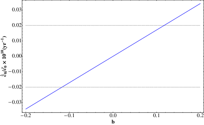
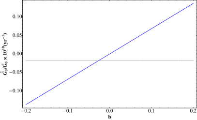
Figure 1: The present values of time variation of physical constants as a function of $b$. a) The values of $\dot{\tilde{c}}_{0}/\tilde{c}_{0}$ multiplied by $10^{10}$ for the different values of $b$ in the units $yr^{-1}$. a) The values of $\dot{\tilde{G}}_{0}/\tilde{G}_{0}$ multiplied by $10^{10}$ for the different values of $b$ in the units $yr^{-1}$.

Eq. (5.13) also should be obtained by differentiating Eq. (5.11) with respect to the cosmic time, $t$ and using Eq. (5.10). This provides the relation between $\tilde{G}$ and $\tilde{c}$ as

$$\frac{d\ln\tilde{G}}{d\ln a}=4\frac{d\ln\tilde{c}}{d\ln a}\equiv b=\text{const.}\quad\Longrightarrow\quad\frac{\tilde{G}}{\tilde{G}_{0}}=\left(\frac{\tilde{c}}{\tilde{c}_{0}}\right)^{4}=\left(\frac{a}{a_{0}}\right)^{b}=a^{b}\,.$$ (5.15)

From the above Eq. (5.15), one can obtain the expressions for the time variations of $\tilde{c}$ and $\tilde{G}$ as

$$\frac{\dot{\tilde{G}}}{\tilde{G}}=bH\quad,\quad\frac{\dot{\tilde{c}}}{\tilde{c}}=\frac{b}{4}H\,.$$ (5.16)

Thus, the present values of both the ratio of the time variation of the gravitational constant and that of the speed of light are given by

$$\frac{\dot{\tilde{G}}_{0}}{\tilde{G}_{0}}=bH_{0}\quad,\quad\frac{\dot{\tilde{c}}_{0}}{\tilde{c}_{0}}=\frac{b}{4}H_{0}\,.$$ (5.17)

One way to obtain the limits on the time variations of both the speed of light and the gravitational constant is by using the evolution of the radius of Mercury [205]. The radius of a planet is determined by the hydrostatic equilibrium equation besides an equation of state and boundary conditions. The presence of the time-varying speed of light causes in general time variations of the radius of a planet. On the other hand, one uses different topographical observations to estimate the actual change in the size of several bodies of the Solar system. There exists a stringent bound for the radius of Mercury. It has not changed more than 1 km in the last $3.9\times 10^{9}$ years [109]. This fact provides a bound for the temporal variation of the speed of light. The hydrostatic equilibrium equation is equivalent to another equation in which the temporal dependence exists only in $G$. The present bound on the time variation of $\tilde{c}$ is $\dot{\tilde{c}}_{0}/\tilde{c}_{0}=0\pm 2\times 10^{-12}\text{yr}^{-1}$ [205]. This provides the bound on $b$ as $-0.11\leq b\leq 0.11$. The present bound on the time variation of $\tilde{G}$ is $\dot{\tilde{G}}_{0}/\tilde{G}_{0}\leq 1.8\times 10^{-12}\text{yr}^{-1}$ [150]. This gives the bound $-0.026\leq b$. We show this in the figure. 1. In the left panel of Fig. 1, the present values of $\dot{\tilde{c}}/\tilde{c}$ for the different values of $b$ are depicted. The value of $\dot{\tilde{c}}_{0}/\tilde{c}_{0}$ is proportional to the present value of the Hubble parameter $H_{0}(\sim 6.83\times 10^{-11})\text{yr}^{-1}$ as shown in Eq. (5.17). The horizontal dotted lines indicate the bound on $\dot{\tilde{c}}_{0}/\tilde{c}_{0}$ in the reference [205]. The sign of $b$ can be determined if $\dot{\tilde{c}}_{0}/\tilde{c}_{0}$ is obtained. We also show the behavior of $\dot{\tilde{G}}_{0}/\tilde{G}_{0}$ as a function of $b$ in the right panel of Fig. 1. Because it is proportional to $H_{0}$ as for the time variation of the speed of light, this behavior is the same as that of $\dot{\tilde{c}}_{0}/\tilde{c}_{0}$ except the slope is increased by factor $4$.

Eq. (5.15) is consistent with Eq. (5.3) and this guarantees the consistency of the theory of meVSL. The above equation (5.15) is one of the main properties of meVSL from which the cosmological evolutions of other quantities are obtained. One adopts Eq. (5.15) into Eq. (5.10) to obtain

$$\rho_{i}=\rho_{i0}a^{-3(1+\omega_{i})-\frac{b}{2}}\equiv\rho_{i\text{rs}}a^{-3(1+\omega_{i})}\,,$$ (5.18)

where we define $\rho_{i\text{rs}}\equiv\rho_{i0}a^{-b/2}$ as the rest-mass density of the $i$-component. Thus, the mass density of $i$-component redshifts slower (faster) than that of the GR for a negative (positive) value of $b$. Or, one can interpret this equation as that the rest mass cosmologically evolves as $a^{-b/2}$. For later use, it is convenient to rewrite the equations  (5.11) and  (5.13) by using Eqs. (5.10) and (5.15)

$$H^{2} =\left(\frac{8\pi\tilde{G}_{0}}{3}\sum_{i}\rho_{i0}a^{-3(1+\omega_{i})}-k\frac{\tilde{c}_{0}^{2}}{a^{2}}\right)a^{\frac{b}{2}}\equiv\left(\frac{8\pi\tilde{G}_{0}}{3}\rho_{\text{cr}}-k\frac{\tilde{c}_{0}^{2}}{a^{2}}\right)a^{\frac{b}{2}}\equiv H^{(\text{GR})2}a^{\frac{b}{2}}\,,$$ (5.19)

$$\frac{\ddot{a}}{a} =\left(-\frac{4\pi\tilde{G}_{0}}{3}\sum_{i}\left(1+3\omega_{i}\right)\rho_{i0}a^{-3(1+\omega_{i})}\right)a^{\frac{b}{2}}+\frac{b}{4}H^{2}$$

$$=\left(-\frac{4\pi\tilde{G}_{0}}{3}\sum_{i}\left(1+3\omega_{i}\right)\rho_{i0}a^{-3(1+\omega_{i})}+\frac{b}{4}H^{(\text{GR})2}\right)a^{\frac{b}{2}}\equiv\left(\left(\frac{\ddot{a}}{a}\right)^{(\text{GR})}+\frac{b}{4}H^{(\text{GR})2}\right)a^{\frac{b}{2}}\,,$$ (5.20)

where we denote $H^{(\text{GR})}$ is the Hubble parameter of GR, $\Lambda\tilde{c}_{0}^{2}=8\pi\tilde{G}_{0}\rho_{\Lambda}$, the equation of state (e.o.s) of the cosmological constant $\omega_{\Lambda}=-1$, and $\rho_{\text{cr}}$ is the critical density to have a flat Universe.

From now on, we limit ourselves to the consideration of the flat universe (i.e., $k=0$) only. In this case, the deceleration parameter, $q$ can be written as

$$q\equiv-\frac{\ddot{a}}{aH^{2}}=\frac{1}{2}\sum_{i}\left(1+3\omega_{i}\right)\Omega_{i}-\frac{b}{4}\equiv q^{(\text{GR})}-\frac{b}{4}\,,$$ (5.21)

where $\Omega_{i}\equiv\rho_{i}/\rho_{\text{cr}}$ is the mass density contrasts of i-component. Because both $H^{2}$ and $\ddot{a}/a$ of meVSL are modified by factor $a^{b/2}$ as shown in Eqs. (5.19) and (5.20), the deceleration parameter does not include an extra scale factor. However, it still includes the meVSL effect as $-b/4$. Thus, the value of the deceleration parameter of meVSL model decreases (increases) by $-b/4$ compared to that of GR when $b$ is positive (negative). This difference is independent of the cosmic time (i.e., the scale factor $a$) and thus gives important information when combined with other observational quantities that depend on the cosmic time.

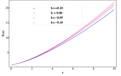
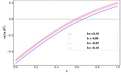
Figure 2: Cosmological evolutions of $E(z)$ and $q(z)$ for the different values of $b$. a) The $E(z)$ for $b=0.1$ (solid), 0 (dotted), -0.05 (dashed), and -0.1 (dot-dashed), respectively. b) $q(z)$ with the same notation as $E(z)$.

One can rewrite the above equations (5.19) and (5.20) by dividing them with $H_{0}^{2}$

$$\frac{H^{2}}{H_{0}^{2}} \equiv E^{2}=\left(\sum_{i}\Omega_{i0}a^{-3(1+\omega_{i})}\right)a^{\frac{b}{2}}\equiv E^{(\text{GR})2}a^{\frac{b}{2}}\,,$$ (5.23)

$$\frac{\ddot{a}}{a}/H_{0}^{2} =\left(-\frac{1}{2}\sum_{i}\left(1+3\omega_{i}\right)\Omega_{i0}a^{-3(1+\omega_{i})}\right)a^{\frac{b}{2}}+\frac{b}{4}E^{(\text{SD})2}a^{\frac{b}{2}}\equiv\left[\left(\frac{\ddot{a}}{a}/H_{0}^{2}\right)^{(\text{GR})}+\frac{b}{4}E^{(\text{GR})2}\right]a^{\frac{b}{2}}\,.$$ (5.24)

Thus, one can find that the present values both $E_{0}$ and $E_{0}^{(GR)}$ are equal to one. However, the present value of the deceleration parameter of meVSL is modified as $q_{0}\equiv-\ddot{a}_{0}/(a_{0}H_{0}^{2})=q_{0}^{(\text{GR})}+b/4$. Thus, the magnitude of the $q_{0}$-value depends on the sign of $b$ too in addition to cosmological parameters. These facts are shown in figure 2. The values of $E(z)$ for the different values of $b$ are shown in the left panel of Fig. 2. Through this manuscript, we adopt best fit cosmological parameters based on Planck 2018 TT + lowE data Planck [248]. The ratio of $E(z)$ of meVSL to that of GR is $(1+z)^{-b/4}$. Thus, $E(z$)-values of meVSL are smaller (bigger) than those of GR for the positive (negative) values of $b$. The dot-dashed, dashed, dotted, and solid lines correspond $b=-0.1,-0.05,0,$ and 0.1, respectively. The percent differences between $E(z)$ and $E^{(\text{GR})}$ at $z=10$ (i.e., $\Delta E(z=10)=(E-E^{(\text{GR})})/E^{(\text{GR})}\times 100(\%)$) $=6.2,3.0$, and $-5.8$ for $b=-0.1,-0.05$, and 0.1, respectively. The cosmological evolutions of values of the deceleration parameter, $q$ of meVSL for different values of $b$ are depicted in the right panel of Fig 2. As shown in Eq. (5.21), the deceleration parameter of meVSL is shifted by $-b/4$ compared to that of GR. Thus, the value of $q$ at the given redshift $z$ decreases as the value of $b$ increases. This induces the delay of late-time acceleration of the Universe as the value of $b$ decreases. Again, the dot-dashed, dashed, dotted, and solid lines correspond b = −0.1, −0.05, 0, and 0.1, respectively. One can define the accelerating redshift, $z_{\text{acc}}$ as $q(z_{\text{acc}})=0$ and $z_{\text{acc}}=0.577,0.597,0.617,$ and 0.658 for $b=-0.1,-0.05,0$, and 0.1, respectively.

One of the main motivations of previous VSL models is providing the model alternative to cosmic inflation by shrinking the so-called comoving Hubble radius in time (i.e., $d(c/aH)/dt<0$). However, one can obtain the comoving Hubble radius of meVSL by using Eqs. (5.15) and (5.19)

$$\frac{\tilde{c}}{aH}=\frac{\tilde{c}_{0}}{aH^{(\text{GR})}}\,.$$ (5.25)

As shown in the above equation (5.25), the Hubble radius of meVSL is the same as that of GR and thus meVSL cannot replace the early inflation.

Now, one can obtain an explicit form of $\tilde{c}$ by using Eqs. (3.2) and (5.19). If the Universe is dominated by the $i$-component, then Eq. (5.19) gives

$$Ht=\frac{2}{3(1+\omega_{i})-b/2}\,.$$ (5.26)

By combining Eqs. (3.2) and  (5.26), one obtains

$$\tilde{c} \equiv\tilde{c}_{0}a^{\frac{b}{4}}=\left(\frac{3(1+\omega_{i})}{3(1+\omega_{i})-b/2}\right)c_{0}a^{\frac{b}{4}}\,,$$ (5.27)

where we assume $c=c_{0}a^{b/4}$. Thus, there exists the upper limit on $b$ as $b<6(1+\omega_{i})$.

5.2 Redshift

The line element of the FLRW metric is given in Eq. (5.1). The proper distance $D_{p}$ from our galaxy ($r=0$) to another galaxy at cosmic time t is given by

$$D_{\text{p}}=a(t)\int_{0}^{r}\frac{dr^{\prime}}{\sqrt{1-kr^{{}^{\prime}2}}}\equiv a(t)f(r)=\begin{cases}a(t)\sin^{-1}r&k=1\\ a(t)r&k=0\\ a(t)\sinh^{-1}r&k=-1\end{cases}\,.$$ (5.28)

Now we consider a light reaching us, at $r=0$, has been emitted from a galaxy at $r=r_{1}$. Also, we consider successive crests of light, emitted at times $t_{1}$ and $t_{1}+\Delta t_{1}$ and received at times $t_{0}$ and $t_{0}+\Delta t_{0}$. Since $ds^{2}=0$ and the light is traveling radially one has for the first and the second crest of light

$$\int_{r_{1}}^{0}\frac{dr}{\sqrt{1-kr^{2}}} =\int_{t_{1}}^{t_{0}}\frac{\tilde{c}dt}{a}=\int_{t_{1}+\Delta t_{1}}^{t_{0}+\Delta t_{0}}\frac{\tilde{c}dt}{a}\,.$$ (5.29)

One can rewrite the above equation as

$$\int_{t_{0}}^{t_{0}+\Delta t_{0}}\frac{\tilde{c}dt}{a} =\int_{t_{1}}^{t_{1}+\Delta t_{1}}\frac{\tilde{c}dt}{a}\quad\Longrightarrow\quad\int_{t_{0}}^{t_{0}+\Delta t_{0}}\frac{\tilde{c}_{0}dt}{a^{1-b/4}}=\int_{t_{1}}^{t_{1}+\Delta t_{1}}\frac{\tilde{c}_{0}dt}{a^{1-b/4}}\,.$$ (5.30)

Now if $\Delta t_{1}$ and $\Delta t_{0}$ are very small (i.e., $\Delta t\ll t$) and then we may assume that $a(t)$ is constant over these intervals, then Eq. (5.30) provides

$$\frac{\Delta t_{1}}{a(t_{1})^{1-b/4}}=\frac{\Delta t_{0}}{a(t_{0})^{1-b/4}}\,.$$ (5.31)

Cosmological redshift is characterized by the relative difference between the observed and emitted wavelengths of an object. This change can be represented by a dimensionless quantity called the redshift, $z$. If $\lambda$ represents wavelength and $\nu$ represents frequency, then the emitted and observed wavelengths are given by

$$\lambda_{\text{e}}\equiv\tilde{c}(t_{1})\Delta t_{1}=\tilde{c}_{0}a_{1}^{b/4}\Delta t_{1}\quad,\quad\lambda_{\text{o}}\equiv\tilde{c}(t_{0})\Delta t_{0}=\tilde{c}_{0}a_{0}^{b/4}\Delta t_{0}\,.$$ (5.32)

If we use Eqs. (5.31) and (5.32), then we obtain

$$1+z\equiv\frac{\lambda_{\text{o}}}{\lambda_{\text{e}}}=\frac{a_{0}}{a_{1}}\,.$$ (5.33)

Thus, the redshift, $z$ in meVSL is the same as that of GR. This is important because the cosmological observations are expressed by using the redshift, not by the cosmic time. If the $z$ of any VSL model is different from that of GR, then one needs to reinterpret the observational data by using a new redshift obtained from that model. In meVSL, as $\tilde{c}$ changes as a function of time, so does the frequency. One can use $\tilde{c}=\tilde{\nu}\lambda$ where $\tilde{\nu}=\tilde{\nu}_{0}a^{b/4}$ by using Eq. (5.31). It means the wavelength is not changed. Also, one can investigate the so-called redshift drift, $\Delta z$, the source redshift changes during the time interval between the first and the second crest of light [249]

$$\Delta z\equiv\frac{a(t_{0}+\Delta t_{0})}{a(t_{1}+\Delta t_{1})}-\frac{a(t_{0})}{a(t_{1})}\approx\Delta t_{0}\left[H_{0}(1+z)-H(t_{1})\frac{\tilde{c}(t_{0})}{\tilde{c}(t_{1})}\right]=\Delta t_{0}\left[H_{0}(1+z)-H(z)^{(\text{GR})}\right]=\Delta z^{(\text{GR})}\,.$$ (5.34)

The redshift drift, $\Delta z$ in meVSL is the same as that of GR. This result is different from other VSL models [47].

5.3 Distances

There are a few different definitions of the distances between two objects or events in the Universe. They are used to relate some observable quantities (such as the redshift of a distant galaxy, the luminosity of a supernova, or the angular size of the acoustic peaks in the CMB power spectrum) to other quantities (like mass density contrast, equation of state of dark energy, and curvature constant) that are not directly observable. We often refer to background observables as cosmological observables related to a distance measurement. It is more practical to write these distances as functions of the redshift, $z$ rather than the cosmic time, $t$. The comoving distance is defined as the distance which is measured locally between two events today if those two points were locked into the Hubble flow. As we show in Eq. (5.29), the comoving distance is defined as

$$D_{\text{C}}(z)\equiv\int_{0}^{r}\frac{dr^{\prime}}{\sqrt{1-kr^{2}}}=\frac{\tilde{c}_{0}}{H_{0}}\int_{0}^{z}\frac{dz^{\prime}}{E^{(\text{GR})}(z^{\prime})}=D_{\text{C}}^{(\text{GR})}(z)\,,$$ (5.35)

where we use the fact that the Hubble radius is identical in both meVSL and GR as shown in Eq. (5.25). Thus, the comoving distances both in GR and in meVSL are the same. The transverse comoving distance is defined as the ratio of the transverse velocity of an object to its proper motion and it is given as

$$D_{\text{M}}(z)=D_{\text{M}}^{(\text{GR})}(z)=\begin{cases}\frac{\tilde{c}_{0}}{H_{0}}\frac{1}{\sqrt{\Omega_{K0}}}\sinh\left(\sqrt{\Omega_{k0}}\frac{H_{0}}{\tilde{c}_{0}}D_{\text{C}}\right)&\Omega_{k0}>0\\ D_{\text{C}}&\Omega_{k0}=0\\ \frac{\tilde{c}_{0}}{H_{0}}\frac{1}{\sqrt{|\Omega_{K0}|}}\sin\left(\sqrt{|\Omega_{k0}|}\frac{H_{0}}{\tilde{c}_{0}}D_{\text{C}}\right)&\Omega_{k0}<0\end{cases}\,.$$ (5.36)

The luminosity distance, $D_{\text{L}}$ is defined by the relationship between bolometric flux and bolometric luminosity. Thus, the relation between the luminosity distance and the transverse comoving distance is modified compared to that of GR as derived in sec. C.6. And the angular diameter distance, $D_{\text{A}}$ is defined as the ratio of an object’s physical transverse size to its angular size. They are given by

$$D_{\text{L}}(z)=(1+z)^{1-b/8}D_{\text{M}}(z)=(1+z)^{-\frac{b}{8}}D_{\text{L}}^{(\text{GR})}(z)\quad,\quad D_{\text{A}}(z)=\frac{D_{\text{M}}}{(1+z)}=D_{\text{A}}^{(\text{GR})}(z)\,.$$ (5.37)

Thus, the so-called cosmic distance duality relation (DDR) of meVSL is different from that of GR and can be written as

$$\frac{(1+z)^{2}D_{\text{A}}}{D_{\text{L}}}=\left(1+z\right)^{-\frac{b}{8}}\,.$$ (5.38)

The comoving volume $V_{\text{C}}$ is defined as the volume measured in which the number densities of non-evolving objects locked into the Hubble flow are constant with redshift. Thus, the comoving volume element in solid angle $d\Omega$ and redshift interval $dz$ is given by

$$\frac{dV_{\text{C}}}{d\Omega dz}=(1+z)^{2}\frac{\tilde{c}_{0}}{H_{0}}\frac{D_{\text{A}}^{2}}{E^{(\text{GR})}(z)}=\left(\frac{dV_{\text{C}}}{d\Omega dz}\right)^{(\text{GR})}\,.$$ (5.39)

Thus, all of the cosmological distances of meVSL are the same as those of GR except the luminosity distance. However, this does not imply that one obtains the same values of cosmological parameters that are extracted from the background evolution observables. This is due to the fact that some physical constants and quantities also vary as a function of the cosmic time as a consequence of a time variation of the speed of light. Thus, we need to investigate subsequent changes in relevant quantities, such as the fine structure constant, the Thomson cross-section, the decay rate of weak interaction, etc, related to physical processes.

6 Observations

The validity of theories of gravity should be verified by cosmological observations. In addition to background evolution observations, there have been various cosmological observations based on the thermal history of the Universe. These include Big Bang Nucleosynthesis (BBN), cosmic microwave background (CMB), baryon acoustic oscillation (BAO), type Ia supernova (SNe), Hubble parameter (H), and gravitational waves (GWs). Also, the time variation of the fine structure constant has been investigated as a possible probe for the time variations of fundamental physical constants. We investigate the effects of meVSL on those cosmological observations in this section.

6.1 BBN

BBN is the formation of primordial light elements other than those of the lightest isotope of hydrogen during the early Universe. At temperatures higher than 1MeV photons, electrons, positrons, neutrinos, antineutrinos, protons, and neutrons formed the primordial plasma of the early Universe. At this epoch, neutrinos start being decoupled and then the number of neutrons begins to diminish through the $\beta$-decay. Neutrons are also captured by protons and form deuterium nuclei. The end result of these reactions was to lock up most of the free neutrons into $\tensor[^{4}]{\text{He}}{}$ nuclei and to create trace amounts of D, $\tensor[^{3}]{\text{He}}{}$, $\tensor[^{7}]{\text{Li}}{}$, and $\tensor[^{7}]{\text{Be}}{}$. One can investigate the modification of meVSL at each mentioned step.

For $T>1$ MeV, a first stage during which the neutrons, protons, electrons, positrons, and neutrinos are kept in statistical equilibrium by the weak interaction. As long as the statistical equilibrium holds, the neutron to proton ratio is

$$\left(\frac{n}{p}\right)=e^{-E_{\text{np}}/k_{\text{B}}T}=\left(\frac{n}{p}\right)^{(\text{GR})}\,,$$ (6.1)

where we use $E_{\text{np}}\equiv(m_{\text{n}\,\text{rs}}-m_{\text{p}\,\text{rs}})\tilde{c}^{2}=(m_{\text{n}0}-m_{\text{p}0})\tilde{c}_{0}^{2}=E_{\text{np}}^{(\text{GR})}=1.293$ MeV. Thus, the neutron to proton ratio in meVSL model is the same as that of GR. The abundance of the other light element of the mass number $A$ and charge $Z$ is given by

$$Y_{A}=g_{A}\left(\frac{\zeta(3)}{\sqrt{\pi}}\right)^{A-1}2^{(3A-5)/2}A^{5/2}\left[\frac{k_{\text{B}}T}{m_{\text{N}}\tilde{c}^{2}}\right]^{3(A-1)/2}\eta^{A-1}Y_{\text{p}}^{Z}Y_{\text{n}}^{A-Z}e^{B_{A}/k_{\text{B}}T}=Y_{A}^{(\text{GR})}\,,$$ (6.2)

where $g_{A}$ is the number of degrees of freedom of the nucleus ${}^{A}_{Z}X$, $m_{\text{N}}$ is the nucleon mass, $\eta$ is the baryon to photon ratio, and $B_{A}\equiv(Zm_{\text{p}}+(A-Z)m_{\text{n}}-m_{A})c^{2}=B_{A}^{(\text{GR})}$ is the binding energy which is identical for both GR and meVSL. Thus, the abundances of light elements are the same in both models.

Around $T\sim 0.8$ MeV, the weak interactions freeze out at a temperature $T_{f}=T(z_{f})$ determined by the competition between the weak interaction rate and the expansion rate of the Universe. The total decay rate of neutrons is given by

$$\Gamma_{\text{w}}=\frac{1}{4\pi^{3}\hbar}\left(\frac{g_{\text{w}}}{2M_{\text{W}}\tilde{c}^{2}}\right)^{4}\left(m_{e}\tilde{c}^{2}\right)^{5}\left[\frac{1}{15}\left(2b^{4}-9b^{2}-8\right)\sqrt{b^{2}-1}+b\ln\left[b+\sqrt{b^{2}-1}\right]\right]\equiv\Gamma_{\text{w}}^{(\text{GR})}a^{\frac{b}{4}}\,,$$ (6.3)

where $g_{\text{w}}$ is the coupling constant of the weak interaction measured as 0.653, $M_{\text{W}}$ is the mass of the W-boson, and $b\equiv(m_{\text{n}}-m_{\text{p}})/m_{\text{e}}\approx 2.53$. $b$ of GR is the same as that of meVSL. In GR, $\Gamma_{\text{w}}^{(\text{GR})}\approx 7.5876\times 10^{-4}s^{-1}$. The decay rate of the neutron is modified from that of GR as shown in Eq. (6.3). However, this does not cause the change of the decoupling epoch of neutrons. The thermal equilibrium of neutrons is maintained so long as the timescale for the weak interaction is short compared with the timescale of the cosmic expansion. They begin to decouple from the primordial plasma when the condition $\Gamma_{\text{w}}\sim H$ is reached. We can show that the decoupling condition of meVSL is equal to that of GR by using Eqs. (5.19) and (6.3)

$$\Gamma_{\text{w}}(z_{f})=H(z_{f})\quad\Longrightarrow\quad\Gamma_{\text{w}}^{(\text{GR})}(z_{f})=H^{(\text{GR})}(z_{f})\,.$$ (6.4)

Thus, the neutrons are decoupled from other elements after $z_{f}$ which is the same for meVSL and GR. After $z_{f}$, the number of neutrons and protons change only through the neutron $\beta$-decay between $T_{f}$ to $T_{\text{N}}\sim 0.1$MeV when $p+n$ reactions proceed faster than their inverse dissociation.

For 0.05 MeV $<T<0.6$MeV, only two-body reactions produce the synthesis of light elements. This requires two conditions. One is that the deuteron to be synthesized ($p+n\rightarrow D$). The other is the very low photon density in order to neglect the photon-dissociation. This happens roughly when

$$\left(\frac{n_{\text{d}}}{n_{\gamma}}\right)\sim\eta^{2}\exp\left[-\frac{B_{\text{D}}}{k_{\text{B}}T}\right]=\left(\frac{n_{\text{d}}}{n_{\gamma}}\right)^{(\text{GR})}\,.$$ (6.5)

The abundance of ⁴He by mass, $Y_{\text{p}}$, is then well estimated by

$$Y_{\text{p}}\simeq 2\frac{(n/p)_{\text{N}}}{1+(n/p)_{\text{N}}}\quad\text{where}\quad\left(\frac{n}{p}\right)_{\text{N}}=\left(\frac{n}{p}\right)_{f}\exp\left[-\frac{t_{\text{N}}}{\tau_{\text{n}}}\right]\,,$$ (6.6)

where $t_{\text{N}}=t_{\text{N}}^{(\text{GR})}(1+z_{\text{N}})^{b/4}$ and $\tau_{\text{n}}=\tau_{\text{N}}^{(\text{GR})}(1+z_{\text{n}})^{b/4}$. This means $Y_{\text{p}}\simeq Y_{\text{p}}^{(\text{GR})}$.

Thus, unlike other VSL models, meVSL does not affect the BBN predictions compared to those of GR. Thus, if one wants to obtain the cosmological limit on the value of $b$, one should use other observations rather than BBN. The same cosmological parameters from BBN based on GR can be adopted in meVSL.

6.2 CMB

CMB is electromagnetic radiation as a remnant from an early Universe after it decouples from the primordial plasma. One can distinguish the recombination from the decoupling. Recombination is the process by which neutral hydrogen is formed via a combination of electrons and protons. At sufficiently low temperatures, photons are no more able to ionize the hydrogen atoms, and thus the number of free electrons dramatically drops. Thus, the epoch of recombination solely depends on the number densities of electrons and protons. The number densities of them are the same both in GR and in meVSL. Thus, the epoch of recombination is not modified in meVSL compared to GR. However, photons interacted primarily with electrons through Thomson scattering (i.e., the elastic scattering of electromagnetic radiation by a free-charged particle). In this process, one can regard the electron as being made to oscillate in the electromagnetic field of the photon causing it, in turn, to emit radiation at the same frequency as the incident wave, and thus the wave is scattered. An important feature of Thomson scattering is that it introduces polarization along the direction of motion of the electron. The cross-section for Thomson scattering is given by

$$\sigma_{\text{T}}=\frac{8\pi}{3}\left(\frac{e^{2}}{4\pi\tilde{\epsilon}m_{\text{e}}\tilde{c}^{2}}\right)^{2}=\sigma_{\text{T}}^{(\text{GR})}a^{-\frac{b}{2}}\,.$$ (6.7)

It is tiny and therefore Thomson scattering is most important when the density of free electrons is high, as in the early Universe or in the dense interiors of stars. The scattering rate per photon, $\Gamma_{\text{T}}$, can be estimated as the speed of light divided by the mean free path for photons (the mean distance traveled between scatterings)

$$\Gamma_{\text{T}}=n_{\text{e}}\sigma_{\text{T}}\tilde{c}=\Gamma_{\text{T}}^{(\text{GR})}a^{-\frac{b}{4}}\,.$$ (6.8)

Thus, the decoupling epoch is determined by using Eqs. (5.19) and (6.8)

$$\Gamma_{\text{T}}=H\quad\Longrightarrow\quad\Gamma_{\text{T}}^{(\text{GR})}=H^{(\text{GR})}a^{\frac{b}{2}}\,.$$ (6.9)

Recombination is the process by which neutral hydrogen is formed via a combination of protons and electrons. Decoupling is generally referred to be the epoch when photons stop interacting with free electrons. In this case, their mean free path becomes larger than the Hubble radius and we are able to detect them as CMB coming from the last scattering surface at the present epoch. We can estimate the deviation of the decoupling epoch in meVSL compared to GR. For this purpose, we assume that the Universe is dominated by the radiation at that epoch, then the Hubble parameter at that epoch is given by $H_{\text{de}}=H_{0}(1+z_{\text{de}})^{2-b/4}$ where $z_{\text{de}}$ is the redshift at the decoupling epoch. Also, if we assume that the Universe is fully ionized at this epoch $n_{\text{e}}(z_{\text{de}})=X_{\text{e}}n_{\text{b}}(z_{\text{de}})=X_{\text{e}}n_{\text{b}0}(1+z_{\text{de}})^{3}$ where $X_{\text{e}}$ is the free electron fraction. Then the decoupling epoch defined to be $\Gamma_{\text{T}}(z_{\text{de}})=H(z_{\text{de}})$ is estimated by

$$\Gamma_{\text{T}}(z_{\text{de}}) =X_{\text{e}}n_{\text{b}}\sigma_{\text{T}}\tilde{c}=\frac{3H_{0}^{2}\Omega_{\text{b}0}}{8\pi\tilde{G}_{0}m_{\text{p}\text{rs}}}X_{\text{e}}\sigma_{\text{T}}^{(\text{GR})}\tilde{c}_{0}\left(1+z_{\text{de}}\right)^{3+\frac{b}{4}}\,,$$ (6.10)

$$\sigma_{\text{T}} =\frac{8\pi}{3}\left(\frac{e^{2}}{4\pi\epsilon m_{\text{e}}\tilde{c}^{2}}\right)^{2}=\frac{8\pi}{3}\left(\frac{e_{0}^{2}}{4\pi\epsilon_{0}m_{\text{e}\text{rs}}\tilde{c}_{0}^{2}}\right)^{2}a^{-\frac{b}{2}}\equiv\sigma_{\text{T}}^{(\text{GR})}a^{-\frac{b}{2}}\,,$$ (6.11)

$$H(z_{\text{de}}) \simeq H_{0}\sqrt{\Omega_{\text{m}0}}\sqrt{1+\frac{1+z_{\text{de}}}{1+z_{\text{eq}}}}(1+z_{\text{de}})^{\frac{3}{2}-\frac{b}{4}}=H_{0}\sqrt{\Omega_{\text{m}0}}\sqrt{1+\left(1+z_{\text{de}}\right)\frac{\Omega_{\text{r}0}h^{2}}{\Omega_{\text{m}0}h^{2}}}(1+z_{\text{de}})^{\frac{3}{2}-\frac{b}{4}}\,,$$ (6.12)

$$\frac{\Gamma_{\text{T}}(z_{\text{de}})}{H(z_{\text{de}})} =\frac{3\sigma_{\text{T}}^{(\text{GR})}\tilde{c}_{0}H_{0}}{8\pi\tilde{G}_{0}m_{\text{p}\text{rs}}h}X_{\text{e}}(z_{\text{de}})\frac{\Omega_{\text{b}0}h^{2}}{\sqrt{\Omega_{\text{m}0}h^{2}}}\left(1+z_{\text{de}}\right)^{\frac{3+b}{2}}\left(1+\left(1+z_{\text{de}}\right)\frac{\Omega_{\text{r}0}h^{2}}{\Omega_{\text{m}0}h^{2}}\right)^{-\frac{1}{2}}\,$$ (6.13)

$$=145\times 33^{b}\times X_{\text{e}}(z_{\text{de}})\left(\frac{\Omega_{\text{b}0}h^{2}}{0.02212}\right)\left(\frac{0.1434}{\Omega_{\text{m}0}h^{2}}\right)^{\frac{1}{2}}\left(\frac{1+z_{\text{de}}}{1090}\right)^{\frac{3+b}{2}}\left(1+\frac{1+z_{\text{de}}}{3411}\frac{0.1434}{\Omega_{\text{m}0}h^{2}}\right)^{-\frac{1}{2}}\,,$$

where $\sigma_{\text{T}}^{(\text{GR})}=6.635\times 10^{-29}\text{m}^{2}$. Thus, the decoupling epoch of meVSL is earlier (later) than that of GR for the negative (positive) value of $b$. The observed decoupling epoch is $z_{\text{de}}=1090$. We show the effect of $b$ on $z_{\text{de}}$ in Fig. 3. The horizontal lines are depicted 1% (dotted), 5% (dot-dashed), 10% (dashed) errors, respectively. As the value of $b$ increases, $z_{\text{de}}$ decreases. If one allows the 1% error in $z_{\text{de}}$, then the allowed range of $b$ is $-0.004\leq b\leq 0.004$. For 5% deviation of $z_{\text{de}}$, $-0.021\leq b\leq 0.022$ is obtained. For 10% deviations of $z_{\text{de}}$, the allowed regions for $b$ is $-0.048\leq b\leq 0.045$.

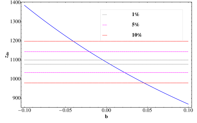
Figure 3: The decoupling redshift as a function of $b$. The horizontal lines correspond 1 (dot-dashed), 5 (dotted), and10 (dashed) % error deviations, respectively.

In the CMB measurement, the shift parameter, $R$ is introduced as a convenient way to quickly evaluate the likelihood of the cosmological models [174]

$$R=\sqrt{\Omega_{\text{m}0}}\int_{0}^{z_{\text{d}}}dz^{\prime}\frac{\tilde{c}(z^{\prime})}{E(z^{\prime})}=\sqrt{\Omega_{\text{m}0}}\int_{0}^{z_{\text{d}}}dz^{\prime}\frac{\tilde{c}_{0}(z^{\prime})}{E^{(\text{GR})}(z^{\prime})}=R^{(\text{GR})}\,.$$ (6.14)

This shift parameter is often used to investigate the VSL model. However, $R$ is the same both in GR and in meVSL. Thus, one is not able to use $R$ to constrain $b$ in meVSL.

The optical depth to Thomson scattering is the integral over time of the scattering rate

$$\tau(t)\equiv\int^{t_{0}}_{t}\Gamma_{\text{T}}(t)dt\,.$$ (6.15)

For instantaneous, complete ionization at redshift $z_{\text{re}}$, one can calculate the optical depth [250]

$$\tau(z_{\text{re}})=(1+y)\frac{(1-Y_{\text{p}})\rho_{\text{cr}0}}{m_{\text{H}0}}\sigma_{\text{T}}^{(\text{GR})}\frac{\tilde{c}_{0}}{H_{0}}\int_{0}^{z_{\text{re}}}\frac{(1+z)^{2+b/2}}{E^{(\text{GR})}(z)}dz\,,$$ (6.16)

where $\rho_{\text{cr}0}$ is the present value of critical density, $m_{\text{H}0}$ is the present mass of hydrogen, and number densities of hydrogen, helium, and electrons are given by $n_{\text{H}}=[(1-Y_{\text{p}})\rho_{\text{cr}0}/m_{\text{H}0}](1+z)^{3}$, $n_{\text{He}}=yn_{\text{H}}$, and $n_{e}=(1+y)n_{\text{H}}$ if helium is singly ionized. The $y$ is related to a helium mass fraction, $Y_{\text{p}}$ by $y=(Y_{\text{p}}/4)/(1-Y_{\text{p}})$. One can obtain the analytic solution of the above integral in Eq. (6.16) if one considers the late time Universe, $E(z)=\sqrt{\Omega_{\text{m}0}(1+z)^{3}+\Omega_{\Lambda 0}}$ with $\Omega_{\Lambda 0}=1-\Omega_{\text{m}0}$

$$\tau(z_{\text{re}}\,,b) =(1+y)\frac{(1-Y_{\text{p}})\rho_{\text{cr}0}}{m_{\text{H}\text{rs}}}\sigma_{\text{T}}^{(\text{GR})}\frac{\tilde{c}_{0}}{H_{0}}\frac{2\Omega_{\text{b}0}}{(6+b)\Omega_{\Lambda 0}}$$

$$\times\Biggl{(}-{}_{2}F_{1}\left[1,\frac{9+b}{6},2+\frac{b}{6},-\frac{\Omega_{\text{m0}}}{\Omega_{\text{$\Lambda$0}}}\right]$$

$$+(1+z_{\text{re}})^{3+\frac{b}{2}}{}_{2}F_{1}\left[1,\frac{9+b}{6},2+\frac{b}{6},-\frac{(1+z_{\text{re}})^{3}\Omega_{\text{m0}}}{\Omega_{\text{$\Lambda$0}}}\right]\sqrt{(1+z_{\text{re}})^{3}\Omega_{\text{m0}}+\Omega_{\text{$\Lambda$0}}}\Biggr{)}\,,$$ (6.17)

where ${}_{2}F_{1}$ is a hypergeometric function and the reionization epoch, $z_{\text{re}}=7.5$ [248]. Eq. (6.17) provides the $\tau(z_{\text{re}})$-dependence on $b$. As $b$ increases, so does $\tau(z_{\text{re}})$. We show this in Fig. 4. In the left panel of Fig. 4, $\tau(z_{\text{re}})$ for the different values of $b$ at the given reionization epoch $z_{\text{re}}$ is depicted. The solid, dotted, dashed, and dot-dashed lines correspond $b=+0.1,0,-0.05$, and $-0.1$, respectively. In Planck 2018 [248], $\tau(7.5)=0.0522\pm 0.0080$ and thus its 1-$\sigma$ error is about 15%. In the right panel of Fig. 4, we show the deviations of $\tau(z_{\text{re}})$ of meVSL from that of GR, $\Delta\tau(z_{\text{re}})=\left(\tau(z_{\text{re}},b\neq 0)-\tau(z_{\text{re}},b=0)\right)/\tau(z_{\text{re}},b=0)\times 100(\%)$. The solid, dashed, and dot-dashed lines correspond $b=+0.1,-0.05$, and $-0.1$, respectively. The differences are about 8 %, -4 %, and -7 % for $b=0.1,-0.05$, and -0.1, respectively. All of these models are within the measurement errors of $\tau(z_{\text{re}})$. Thus, the current observational accuracy on the optical depth might not provide a strong constraint on $b$.

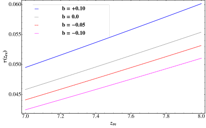
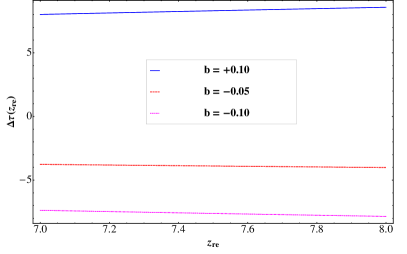
Figure 4: The optical depth to the reionization for the different values of $b$. a) The optical depth, $\tau(z_{\text{re}})$ for $b=+0.1$(solid), 0 (dotted), -0.05 (dashed), and -0.1 (dot-dashed), respectively. b) The differences of $\tau(z_{\text{re}})$ between meVSL models and GR (i.e., $b=0$).

The conformal time derivative of the optical depth, $\tau^{\prime}$ and the visibility function are given by

$$\tau^{\prime} \equiv\frac{d\tau}{d\eta}=-n_{\text{e}}\sigma_{\text{T}}a\tilde{c}=\tau^{{}^{\prime}(\text{GR})}a^{-\frac{b}{4}}\,,$$ (6.19)

$$g(\eta) \equiv-\tau^{\prime}e^{-\tau}\quad\text{with}\quad\int_{0}^{\eta_{0}}d\eta g(\eta)=1\,.$$ (6.20)

These quantities contribute to the source terms of temperature and polarization. However, the visibility function is nonzero only during the recombination and reionization process. Thus, it provides a weak constraint on $b$.

6.3 SZE

Masses of clusters of galaxies often exceed $3\times 10^{14}M_{\odot}$ with the effective gravitational radii, $R_{\text{eff}}$ of order Mpc. Any gas in hydrostatic equilibrium within a cluster’s gravitational potential well has electrons with the temperature $T_{e}$ given by

$$k_{\text{B}}T_{\text{e}} \approx\frac{GMm_{\text{p}}}{2R_{\text{eff}}}=6.74\left(\frac{M}{3\times 10^{14}M_{\odot}}\right)\left(\frac{\text{Mpc}}{R_{\text{eff}}}\right)\text{KeV}\,,$$ (6.21)

where $G=4.3\times 10^{-3}$ pc $\text{M}_{\odot}^{-1}$ $\left(\text{km}/\text{s}\right)^{2}$ and $m_{\text{p}}$ = 938.272 MeV/$c^{2}$. At this temperature, the X-ray part of the spectrum shows the thermal emission from the gas which is composed of thermal bremsstrahlung and line radiation.

Among the mass of clusters of galaxies, the mass of distributed gas is about a quarter of it. Thus, clusters of galaxies are luminous X-ray sources, with the bulk of the X-rays being produced as bremsstrahlung rather than line radiation due to this high mass density of the gas. However, electrons in the intracluster gas are scattered not only by ions but also CMB photons. The cross-section of this low-energy scattering is given by the Thomson scattering cross-section, $\sigma_{\text{T}}$ so that the scattering optical depth $\tau_{\text{e}}\simeq n_{\text{e}}\sigma_{\text{T}}R_{\text{eff}}\sim 10^{-2}$. Due to the inverse Thomson scattering with the high-temperature electrons, the frequency of the photon will be shifted slightly and upscattering is more presumably. On average a slight mean change of photon energy from this scattering is produced

$$\frac{\Delta\nu}{\nu}\approx\frac{k_{\text{B}}T_{\text{e}}}{m_{\text{e}}c^{2}}\sim\frac{6.74KeV}{0.511MeV}\sim 1.32\times 10^{-2}\,.$$ (6.22)

Thus, this inverse Compton (Thomson) scattering produces about 1 part in $10^{4}$ overall change in brightness of CMB.

Spatial distributions of clusters of galaxies determine SZE. SZE is observed towards clusters of galaxies which are large-scale structures detectable in the optical and X-ray bands and it is localized. In addition, other observable properties of the clusters also affect the amplitude of the signal. However, primordial structures of the CMB are nonlocalized. They are also not related to structures seen at different wavebands. Moreover, they are randomly distributed over the entire sky with almost constant correlation amplitude in different patches of sky. When the radiation passes through an electron population with significant energy content, its spectrum is distorted. This is called the thermal SZE.

One can express the scattering optical depth, Comptonization parameter, and X-ray spectral surface brightness along a particular line of sight with a cluster atmosphere gas of electron concentration $n_{\text{e}}({\bf r})$

$$\tau_{\text{e}} =\int n_{\text{e}}({\bf r})\sigma_{\text{T}}dl\,,$$ (6.23)

$$y =\int n_{\text{e}}({\bf r})\sigma_{\text{T}}\frac{k_{\text{B}}T_{\text{e}}({\bf r})}{d}l\,,$$ (6.24)

$$S_{X}(E) =\frac{1}{4\pi(1+z)^{3}}\int n_{\text{e}}({\bf r})^{2}\Lambda(E,T_{\text{e}})dl\,,$$ (6.25)

where $z$ is the redshift of the cluster, and $\Lambda$ is the spectral emissivity of the gas at observed X-ray energy $E$. One obtains the factor of $4\pi$ from the assumption of the isotropic emissivity. Also, the cosmological transformations of spectral surface brightness and energy give the $(1+z)^{3}$ factor. Introducing a parameterized gas model in the cluster and using it to fit these parameter values to the X-ray data is convenient in many cases. One can predict the appearance of the cluster in the SZE by integrating Eq. (6.24). There exists a simple and popular model called the isothermal $\beta$ model. In this model, the electron temperature, $T_{\text{e}}$ is regarded as a constant, and the electron number density is assumed as spherically distributed

$$n_{\text{e}}({\bf r})=n_{\text{e}0}\left(1+x^{2}\right)^{-\frac{3}{2}\beta}\,,$$ (6.26)

where $x=r/r_{c}$ and $r_{c}=\theta_{\text{c}}D_{\text{A}}$ is the core radius of the distribution. The surface brightness profile of intracluster medium observed at the projected radius, $b_{\text{p}}$, $S_{X}(b_{\text{p}})$, is the projection on the sky of the plasma emissivity, $\epsilon(r)$

$$S_{X}(b_{\text{p}}) =\frac{1}{4\pi}\frac{D_{\text{A}}^{2}}{D_{\text{L}}^{2}}\int_{b^{2}}^{\infty}\frac{\epsilon dr^{2}}{\sqrt{r^{2}-b_{\text{p}}^{2}}}\quad,\text{where}\quad\epsilon(r)=\Lambda(T_{gas})n_{p}^{2}\quad\left(\text{ergs}^{-1}\text{cm}^{-3}\right)$$

$$=\frac{1}{4\sqrt{\pi}}\frac{1}{(1+z)^{4}}n_{0}^{2}\Lambda(T_{gas})r_{c}\frac{\Gamma[3\beta-\frac{1}{2}]}{\Gamma[3\beta]}\left(1+\frac{b_{\text{p}}^{2}}{r_{c}^{2}}\right)^{0.5-3\beta}\equiv S_{0}\left(1+\frac{b_{\text{p}}^{2}}{r_{c}^{2}}\right)^{0.5-3\beta}\,,$$ (6.27)

where $n_{\text{p}}=\rho_{\text{gas}}/(2.21\mu m_{\text{p}})$ is the proton density and the cooling function, $\Lambda(T_{\text{gas}})$ depends on the mechanism of the emission. Assuming isothermality and a $\beta$-model for the gas density, the surface brightness profile has an analytic solution. The SZE on the temperature is given by

$$\Delta T_{\text{SZE}}(\theta) =f(\nu,T_{\text{e}})\frac{k_{\text{B}}T_{\text{e}}T_{\gamma 0}}{m_{\text{e}\rm}\tilde{c}_{0}^{2}}\sigma_{\text{T}}^{(\text{GR})}(1+z)^{\frac{b}{2}}\int_{-l_{max}}^{l_{max}}n_{e}dl=f(\nu,T_{\text{e}})\frac{k_{\text{B}}T_{\text{e}}T_{\gamma 0}}{m_{\text{e}\rm}\tilde{c}_{0}^{2}}\sigma_{\text{T}}^{(\text{GR})}(1+z)^{\frac{b}{2}}\int_{b^{2}}^{\infty}\frac{n_{e}dr^{2}}{\sqrt{r^{2}-b_{\text{p}}^{2}}}\,,$$

$$=f(\nu,T_{\text{e}})\frac{k_{\text{B}}T_{\text{e}}T_{\gamma 0}}{m_{\text{e}\rm}\tilde{c}_{0}^{2}}\sigma_{\text{T}}^{(\text{GR})}(1+z)^{\frac{b}{2}}\sqrt{\pi}n_{0}r_{c}\frac{\Gamma[\frac{3\beta-1}{2}]}{\Gamma[\frac{3\beta}{2}]}\left(1+\frac{b_{\text{p}}^{2}}{r_{c}^{2}}\right)^{\frac{1-3\beta}{2}}\equiv\Delta T_{0}\left(1+\frac{b_{\text{p}}^{2}}{r_{c}^{2}}\right)^{\frac{1-3\beta}{2}}\,,$$ (6.28)

where $S_{0}$, $\Delta T_{0}$, and $\theta_{\text{c}}$ are observed quantities. Thus, one can solve for $n_{0}$ from Eqs. (6.27) and (6.28) to obtain $D_{\text{A}}$

$$D_{A}(z_{\text{c}})=\frac{1}{4\pi\sqrt{\pi}}\left[\frac{\Delta T_{0}^{2}}{S_{X0}}\theta_{\text{c}}^{-1}\frac{\tilde{\Gamma}[\beta]}{\tilde{\Gamma}[\beta/2]^{2}}\right]\left[\left(\frac{m_{\text{e}\text{rs}}\tilde{c}_{0}^{2}}{k_{\text{B}}T_{\text{e}0}}\right)\frac{\Lambda}{fT_{\gamma 0}\sigma_{\text{T}}^{(\text{GR})}}\right]^{2}\left(1+z_{\text{c}}\right)^{-4-b}\equiv D_{\text{A}}^{(\text{GR})}(z_{\text{c}})(1+z_{c})^{-b}\,,$$ (6.29)

where $\tilde{\Gamma}[\beta]=\Gamma[3\beta-1/2]/\Gamma[3\beta]$. Thus, the observed diameter distance has extra $(1+z_{c})^{-b}$ factor in meVSL compared to GR. The difference between GR and meVSL is given by

$$\Delta D_{A}(z_{\text{c}})\equiv\frac{D_{A}(z_{\text{c}})-D_{A}^{(\text{GR})}(z_{\text{c}})}{D_{A}^{(\text{GR})}(z_{\text{c}})}=\left(1+z_{\text{c}}\right)^{b}-1\,.$$ (6.30)

We show the behavior of this in Fig. 5. It is obvious that $\Delta D_{A}(z_{\text{c}})$ increases as $z_{\text{c}}$ does. The dot-dashed, dotted, and solid lines correspond $b=-0.1,-0.05$, and $0.1$, respectively. The discrepancies are about 2% and 4 (-4)% at $z_{c}=0.5$ for $b=-0.05$ and -0.1 (+0.1), respectively. Thus, one needs to consider the time-varying speed of light effect when one interprets the cosmological parameters from the observed angular diameter obtained from the X-ray cluster.

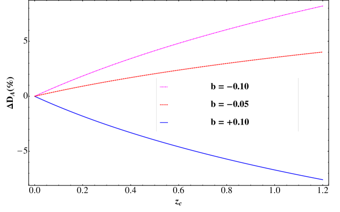
Figure 5: The differences of angular diameter distance between meVSL and GR, $\Delta D_{\text{A}}(z_{c})$ as a function of $z_{c}$ for different values of $b$. The dot-dashed, dashed, and solid lines correspond $b=-0.1,-0.05$, and 0.1, respectively.

6.4 BAO

The oscillating behavior of primordial plasma is created by the competition between the gravitational attraction of matter to the primordial plasma and the outward pressure created from the heat of photon-matter interactions. This overdense region contains dark matter (DM), baryons, and photons. The pressure results in spherical sound waves of both baryons and photons outwards from the overdensity. While the DM interacts with other components only gravitationally, and thus it stays at the center of the sound waves. The photons and baryons moved outwards together before decoupling. However, they diffused away after the decoupling due to the lack of interactions between the photons and the baryons. That provided the pressure on the system, leaving behind shells of baryonic matter. Out of all those shells, representing different sound waves wavelengths, the resonant shell corresponds to the first one as it is that shell that travels the same distance for all overdensities before decoupling. The radius of this traveling distance is called the sound horizon. There remains only the gravitational force acting on the baryons after the disappearance of the photon-baryon pressure driving the system outwards. Hence, the baryons and DM constructed a shape that comprised overdensities of matter both at the original position of the anisotropy and in the shell at the sound horizon for that anisotropy.

Such anisotropies eventually became the ripples in matter density that would form galaxies. Thus, it is expected that there exist a greater number of galaxy pairs at the sound horizon distance scale compared to at other length scales. This specific pattern of matter happened at each anisotropy in the early universe to make many overlapping ripples.

The effect of baryon loading on the CMB monopole is given by

$$\int_{0}^{\eta_{\text{drag}}}kc_{s}(\eta^{\prime})d\eta^{\prime}\equiv kr_{s}(\eta_{\text{drag}})\,,$$

$$r_{s}(\eta_{\text{drag}})=\int_{0}^{\eta_{\text{drag}}}\tilde{c}_{s}d\eta=\int_{z_{\text{drag}}}^{\infty}\frac{\tilde{c}_{s}}{H}dz=\int_{z_{\text{drag}}}^{\infty}\frac{\tilde{c}_{s}^{(\text{GR})}}{H^{(\text{GR})}}\sqrt{\frac{1+R}{1+\frac{1+b/6}{1+b/8}R}}dz\neq r_{s}^{(\text{GR})}(\eta_{\text{drag}})\,,$$ (6.31)

where $r_{s}$ is the sound horizon evaluated at the baryon drag epoch and the speed of sound of the baryon-photon plasma, $\tilde{c}_{s}$ is given by

$$\tilde{c}_{s}^{2} \equiv\frac{\partial P}{\partial\rho}=\frac{\tilde{c}_{0}^{2}}{3}a^{\frac{b}{2}}\left(1+\frac{(3+b/2)\rho_{b}}{(4+b/2)\rho_{\gamma}}\right)^{-1}\equiv\tilde{c}_{s}^{(GR)2}a^{\frac{b}{2}}\frac{1+R}{1+\frac{1+b/6}{1+b/8}R}\quad\text{where}\quad R=\frac{3\rho_{b}}{4\rho_{\gamma}}\,.$$ (6.32)

Thus, there exits difference on the sound horizon between of GR and of meVSL.

Galaxy distribution is three dimensional and thus one measurement of the sound horizon should be done in three different directions. Two of them are on the projected sky and the other is in the radial direction [215]. The former is referred to be the tangential modes and the latter is the radial defined as

$$y_{\text{t}}(z) =\frac{D_{\text{A}}(z)}{r_{s}(z_{\text{drag}})}\quad\text{and}\quad y_{\text{r}}(z)=\frac{c}{H(z)r_{s}(z_{\text{drag}})}\,.$$ (6.33)

Thus, one can measure the constraint on the value of $b$ from the measurements of tangential and radial modes. However, if we limit the measurements as the combined quantities using $D_{A}$ and $H$, as, for example, the cube root of the product of the radial dilation times the square of the transverse dilation, the average distance [251]

$$D_{V}=\left[(1+z)^{2}\frac{cz}{H}D_{A}^{2}\right]^{1/3}=\left[\frac{cz}{H}D_{\text{M}}^{2}\right]^{1/3}=\left[\frac{\tilde{c}_{0}z}{H^{(\text{GR})}}D_{\text{M}}^{(\text{GR})2}\right]^{1/3}=D_{V}^{(\text{GR})}\,,$$ (6.34)

or the Alcock-Paczynski (AP) distortion parameter

$$F=(1+z)D_{A}\frac{H}{c}=(1+z)D_{A}^{(\text{GR})}\frac{H^{(\text{GR})}}{\tilde{c}_{0}}=F^{(\text{GR})}\,.$$ (6.35)

Thus, both $D_{V}$ and $F$ are same in both GR and meVSL. Thus, one is not able to use either the average distance or the AP to distinguish between GR and meVSL.

In order to investigate dark energy, the low redshift constraints on the path from today, $z=0$ to the galaxy, $z=z_{1}$ are investigated rather than $z_{1}$ to the last scattering surface. For this purpose, in the literature one often adopts the so-called the BAO shift parameter $A(z_{1})$ at a specific $z_{1}$ which is defined as [251]

$$A(z_{1}) \equiv D_{V}(z_{1})\frac{\sqrt{\Omega_{m0}}H_{0}}{z_{1}c}\equiv\left(\frac{\sqrt{\Omega_{m0}}}{E^{(\text{GR})}(z_{1})}\right)^{\frac{1}{3}}\left[\frac{\sqrt{\Omega_{m0}}}{z_{1}}\int_{0}^{z_{1}}\frac{dz^{\prime}}{E^{(\text{GR})}(z^{\prime})}\right]^{\frac{2}{3}}\left(1+z_{1}\right)^{-\frac{b}{4}}$$

$$\equiv A^{(\text{GR})}(z_{1})(1+z_{1})^{-\frac{b}{4}}\,.$$ (6.36)

As shown in the above equation  (6.36), the BAO shift parameter of meVSL deviates from that of GR. Thus, one might need to take into account the varying c in this observable. We show the values of $A(z_{1})$ for different models in the left panel of Fig. 6. The dot-dashed, dashed, dotted, and solid lines correspond $b=-0.1,-0.05,0,$ and +0.1, respectively. The deviations of $A(z_{1})$ for $b\neq 0$ from that of $b=0$ are depicted in the right panel of Fig. 6. $\Delta A(z_{1})\equiv(A(z_{1})-A^{(\text{GR})}(z_{1}))/A^{(\text{GR})}(z_{1})\times 100$ % and they are all sub-percentage level for $-0.1\leq b\leq 0.1$. Thus, even though there do exist the differences in $A(z_{1})$ between GR and meVSL, they might be ignored with the given measurement accuracy [217].

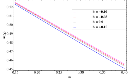
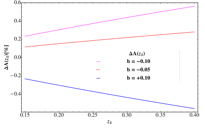
Figure 6: The BAO shift parameters for different models. a) The shift parameter, $A(z_{1})$ at $z_{1}$ for different values of $b$. b) The difference of the BAO shift parameter, $\Delta A(z_{1})$ for the different values of $b$.

6.5 SNe

Supernovae are promising candidates for measuring cosmic expansion. Their peak brightnesses seem quite uniform, and they are bright enough to be seen at extremely large distances. The type Ia supernovae (SNe Ia) show a great uniformity both in their spectral characteristics and in their light curves that are in the way their luminosities vary as functions of time, as they reach the peak of brightness first and then fade over after around a few weeks. Thus, they are regarded as standard candles.

SNe Ia are thought to be nuclear explosions of WDs in binary systems. The WD gradually cumulate matter from an evolving companion and its mass reaches toward the Chandrasekhar limit. WDs resist against gravitational collapse mainly through the electron degeneracy pressure. The Chandrasekhar limit denotes the mass above which the gravitational self-attraction of the star becomes strong enough to overcome the electron degeneracy pressure in the star’s core. Consequently, a WD with a mass greater than this limit is subject to further gravitational collapse, evolving into a different type of stellar remnant, such as a neutron star or black hole. Those with masses up to this limit remain stable as WDs. Based on the equation of state for an ideal Fermi gas, the Chandrasekhar mass limit, $M^{(\text{Ch})}$ is given by,

$$M^{(\text{Ch})} =\frac{\omega_{3}^{0}\sqrt{3\pi}}{2}\left(\frac{\hbar\tilde{c}}{\tilde{G}}\right)^{\frac{3}{2}}\frac{1}{\left(\mu_{e}m_{\text{H}}\right)^{2}}=\frac{\omega_{3}^{0}\sqrt{3\pi}}{2}\left(\frac{\hbar\tilde{c}_{0}}{\tilde{G}_{0}}\right)^{\frac{3}{2}}\frac{1}{\left(\mu_{e}m_{\text{H}0}\right)^{2}}a^{-\frac{b}{2}}\equiv M^{(\text{Ch})}_{0}a^{-\frac{b}{2}}\,,$$ (6.38)

where $\omega_{0}^{3}\approx 2.018$ is a constant related with the solution to the so-called Lane-Emden equation, $\mu_{e}$ is the average molecular weight per electron which is determined by the chemical composition of the star, and $m_{\text{H}0}$ is the present value of the mass of the hydrogen atom.

Figure 7: The distance module, $\mu$ and the difference of distance module, $\Delta\mu$ for the different values of $b$.

The peak luminosity is proportional to the mass of synthesized nickel in the simple analytic light curve models. And this mass is a fixed fraction of the Chandrasekhar mass to a good approximation. The actual fraction varies when different specific SNe Ia scenarios are considered, but the physical mechanisms relevant for SNe Ia naturally relates the energy yield to the Chandrasekhar mass. Thus, the peak luminosity of SNe Ia is proportional to the total amount of nickel synthesized in the SN outburst, $L\propto M^{(\text{Ch})}$. We define that the apparent magnitude of a star would be equal to its absolute magnitudeIf when the star was at $10$ parsecs distance from us. Thus, the absolute magnitude is a measure of the star’s luminosity $\text{M}\propto-2.5\log[L]$. Under this assumption, we have the modification of the absolute magnitude of SNe Ia

$$\text{M}-\text{M}_{0}=-2.5\log\left[\frac{L}{L_{0}}\right]=\frac{5}{4}b\log\left[a\right]\,,$$ (6.40)

where the subscript $0$ refers to the local value of $M$. Thus, the distance module of meVSL, $\mu$ is written by

$$\mu=5\log\left[\frac{D_{\text{L}}}{1\text{Mpc}}\right]+25+\frac{5}{4}b\log\left[a\right]=\mu^{(\text{GR})}-\frac{5}{4}b\log\left[1+z\right]\,,$$ (6.41)

where $D_{\text{L}}$ is the luminosity distance given in Eq. (5.37). Thus, one might have a measurement error in the distance module when one assumes the Universe is governed by GR instead of meVSL by $-\frac{5}{4}b\log\left[1+z\right]$. The larger the redshift, the greater the deviation. We show this in Fig. 7. The left panel of Fig. 7 shows the distance modules for the different models. The dot-dashed, dashed, dotted, and solid lines correspond $b=-0.1,-0.05,0$, and $0.1$, respectively. The differences in distance modules, $\mu-\mu^{(\text{GR})}$ are depicted in the right panel of Fig.7. $\Delta\mu$ can be 0.04 (0.02, -0.04) for $b=-0.1(-0.05,0.1)$ at $z=1.2$. These are quite small and SNe Ia are improper observation to constrain $b$ [220]. This result is rather different from that of [192, 142, 146, 107, 193, 194, 50]

6.6 GWs

If it is somehow possible to learn how the source’s mass quadrupole moment varies with time, then a measurement of the gravitational wave (GW) amplitude would reveal that distance by using the fact that the amplitude of a GW falls off inversely with the distance to the source, $h_{jk}=2G/(c^{4}D)\ddot{I}_{jk}$. Thus, the GWs generated by the merger of two massive compact objects give the information of the distance to the merger and providing the independent distance measurement method. Thus, the measurement of the luminosity distance with standard sirens is one of the most interesting targets of third-generation GW detectors.

The waveform produced by a binary inspiral is modified by the propagation across cosmological distance. In a local wave zone, where the distance to the source is sufficiently large so that the gravitational field already has the $1/r$ behavior characteristic of waves, but still sufficiently small, so that the expansion of the Universe is negligible. The GW produced at a distance $r_{\text{phys}}=a(t_{\text{emis}})r$ in the local wave zone is written as

$$h_{+}\left(t_{\text{s}}\right) =h_{\text{c}}(t^{\text{ret}}_{\text{s}})\frac{1+\cos^{2}\imath}{2}\cos\left[2\Phi\left(t^{\text{ret}}_{\text{s}}\right)\right]\quad,\quad h_{\times}\left(t_{\text{s}}\right)=h_{\text{c}}(t^{\text{ret}}_{\text{s}})\cos\imath\cos\left[2\Phi\left(t^{\text{ret}}_{\text{s}}\right)\right]\,\quad,\quad\text{where}$$ (6.42)

$$h_{\text{c}}(t^{\text{ret}}_{\text{s}}) =\frac{4}{a(t_{\text{emis}})r}\left(\frac{GM_{\text{chirp}}}{\tilde{c}^{2}}\right)^{\frac{5}{3}}\left(\frac{\pi f^{(\text{s})}_{\text{gw}}(t^{\text{ret}}_{\text{s}})}{\tilde{c}}\right)^{\frac{2}{3}}=\frac{4}{a(t_{\text{emis}})r}\left(\frac{G^{(\text{GR})}M_{\text{chirp}}^{(\text{GR})}}{\tilde{c}_{0}^{2}}\right)^{\frac{5}{3}}\left(\frac{\pi f^{(\text{s})(\text{GR})}_{\text{gw}}(t^{\text{ret}}_{\text{s}})}{\tilde{c}_{0}}\right)^{\frac{2}{3}}a^{-\frac{1}{16}b}\,,$$

$$=h_{\bar{c}}^{(\text{GR})}(t^{\text{ret}}_{\text{s}})a^{-\frac{1}{16}b}\,$$ (6.43)

$$f^{(\text{s})}_{\text{gw}}(\tau_{\text{s}}) =\frac{1}{\pi}\left(\frac{5}{256}\frac{1}{\tau_{\text{s}}}\right)^{\frac{3}{8}}\left(\frac{GM_{\text{chirp}}}{\tilde{c}^{3}}\right)^{-\frac{5}{8}}=\frac{1}{\pi}\left(\frac{5}{256}\frac{1}{\tau_{\text{s}}}\right)^{\frac{3}{8}}\left(\frac{G^{(\text{GR})}M_{\text{chirp}}^{(\text{GR})}}{\tilde{c}_{0}^{3}}\right)^{-\frac{5}{8}}a^{\frac{5}{32}b}\equiv f^{(\text{s})(\text{GR})}_{\text{gw}}(\tau_{\text{s}})a^{\frac{5}{32}b}\,,$$ (6.44)

$$M_{\text{chirp}} =\mu^{\frac{3}{5}}m^{\frac{2}{5}}=M_{\text{chirp}}^{(\text{GR})}a^{-\frac{b}{2}}\quad\text{where}\quad\frac{1}{\mu}=\frac{1}{m_{1}}+\frac{1}{m_{2}}=\frac{1}{\mu^{(\text{rs})}}a^{\frac{b}{2}}\,\,,\,\,m\equiv m_{1}+m_{2}=m^{(\text{rs})}a^{-\frac{b}{2}}\,,$$ (6.45)

$$\Phi\left(t^{\text{ret}}_{\text{s}}\right) =\pi\int^{t^{\text{rs}}_{\text{s}}}dt^{\prime}_{\text{s}}f^{(\text{s})}_{\text{gw}}(t_{\text{s}}^{\prime})\,,$$ (6.46)

where $\imath$ is the angle between the observer’s $z$-axis and the normal to the orbit, $\tau\equiv t_{\text{coal}}-t$ is the time to coalescence, $t_{\text{s}}$ is the time measured by the clock of the source, $t^{\text{ret}}_{\text{s}}$ is the corresponding value of retarded time, $t_{\text{emis}}$ is the time of emission, $h_{\text{c}}$ is the amplitude of GW, $M_{\text{chirp}}$ is the chirp mass, $f_{\text{gw}}$ is the angular frequency of the GW which is twice the orbital frequency, and $\Phi$ is the integrated phase. Thus, both the amplitude and the phase measured by the clock of the source are modified in meVSL. However, we measure GW at present and we need to replace the above results in the observer’s time.

After propagation from the source to the detector, the GW amplitude is given by the above equations  (6.42)-(6.46) with replacing $a(t_{\text{emis}})$ by $a(t_{0})$. Then, it is convenient to express the above results in terms of the time, $t_{\text{obs}}=(1+z)t_{\text{s}}$ and the GW frequency, $f^{\text{obs}}_{\text{gw}}=f^{\text{s}}/(1+z)$ measured by the observer. Both Eqs. (6.43) and (6.44) are rewritten by

$$h_{\text{c}}(t^{\text{ret}}_{\text{obs}}) =\frac{4}{a(t_{0})r}(1+z)^{\frac{2}{3}}\left(\frac{G^{(\text{GR})}M_{\text{chirp}}^{(\text{GR})}}{\tilde{c}_{0}^{2}}\right)^{\frac{5}{3}}\left(\frac{\pi f^{(\text{obs})(\text{GR})}_{\text{gw}}(t^{\text{ret}}_{\text{obs}})}{\tilde{c}_{0}}\right)^{\frac{2}{3}}\,,$$

$$\equiv\frac{4}{D_{\text{L}}(z)}\left(\frac{G^{(\text{GR})}\mathcal{M}_{\text{chirp}}^{(\text{GR})}(z)}{\tilde{c}_{0}^{2}}\right)^{\frac{5}{3}}\left(\frac{\pi f^{(\text{obs})(\text{GR})}_{\text{gw}}(t^{\text{ret}}_{\text{obs}})}{\tilde{c}_{0}}\right)^{\frac{2}{3}}=h_{\bar{c}}^{(\text{GR})}(t^{\text{ret}}_{\text{s}})\,,$$ (6.47)

$$f^{(\text{obs})}_{\text{gw}}(\tau_{\text{obs}}) =\frac{1}{\pi}\left(\frac{5}{256}\frac{1}{\tau_{\text{obs}}}\right)^{\frac{3}{8}}\left(\frac{G^{(\text{GR})}\mathcal{M}_{\text{chirp}}^{(\text{GR})(z)}}{\tilde{c}_{0}^{3}}\right)^{-\frac{5}{8}}\equiv f^{(\text{obs})(\text{GR})}_{\text{gw}}(\tau_{\text{obs}})\,,$$ (6.48)

where $D_{\text{L}}$ is the luminosity distance given in Eq. (5.37). We use $a_{\text{obs}}=a_{0}=1$ and define $\mathcal{M}_{\text{chirp}}(z)=(1+z)M_{\text{chirp}}$. Also we can use $\mathcal{M}_{\text{chirp}}(z_{\text{obs}})=M_{\text{chirp}}$. Thus, the observed $h_{\text{c}}$ and $f_{\text{gw}}^{\text{obs}}(\tau_{\text{obs}})$ of meVSL are same as those of GR.

However, we still have the effect of meVSL on the GWs detection. As we show in the appendix. C.7, the propagation equation of the TT gauge metric perturbations, $h$ in the FLRW background is given by Eq. (C.79)

$$h^{\prime\prime}+2\mathcal{H}\left(1+\frac{b}{8}\right)h^{\prime}+\tilde{c}^{2}k^{2}h=0\,,$$ (6.49)

where $h(\eta,{\bf k})$ are the Fourier modes of the GW amplitudes, primes denote the derivative with respect to the conformal time, and $\mathcal{H}=a^{\prime}/a$. However, we need to replace the conformal time derivatives in the above equation. (6.49) with the derivatives w.r.t to $\ln a$ in order to properly investigate the modification of GW evolutions in meVSL. Then the above equation is rewritten as

$$\frac{d^{2}h}{d\ln a^{2}}+\left(2+\frac{\mathcal{H}^{\prime}}{\mathcal{H}^{2}}+\frac{b}{4}\right)\frac{dh}{d\ln a}+\frac{\tilde{c}^{2}k^{2}}{\mathcal{H}^{2}}h=\frac{d^{2}h}{d\ln a^{2}}+\left(2+\frac{\mathcal{H}^{\prime}}{\mathcal{H}^{2}}+\frac{b}{4}\right)\frac{dh}{d\ln a}+\frac{\tilde{c}_{0}^{2}k^{2}}{\mathcal{H}^{(\text{GR})2}}h=0\,,$$ (6.50)

where $\mathcal{H}^{\prime}/\mathcal{H}^{2}\equiv-q=-q^{(\text{GR})}+b/4$ as given in Eq. (5.21). Thus, the above equation is rewritten as

$$\frac{d^{2}h}{d\ln a^{2}}+\left(2-q^{(\text{GR})}+\frac{b}{2}\right)\frac{dh}{d\ln a}+\frac{\tilde{c}_{0}^{2}k^{2}}{\mathcal{H}^{(\text{GR})2}}h=0\,,$$ (6.51)

the source-term is the same as that of GR because $\tilde{c}=\tilde{c}_{0}a^{b/4}$, $\mathcal{H}=\mathcal{H}^{(GR)}a^{b/4}$, and the wavenumber $k$ is a constant. However, the Hubble friction term are different from that of GR by the extra-term, $b/2$. Thus, there exists the varying-$\tilde{c}$ effect only on the friction term in the meVSL. Thus, this change affects the luminosity distance of GW which affects the amplitude of GWs, $h_{\text{c}}$ as shown in Eq. (6.47). One can define $h$ as $Ae^{iB}$ and insert it into Eq. (6.49) to obtain

$$\frac{A^{\prime\prime}}{A}+\left(2+\frac{b}{4}\right)\mathcal{H}\frac{A^{\prime}}{A}-B^{{}^{\prime}2}+\tilde{c}^{2}k^{2}=0\,,$$ (6.52)

$$2\frac{A^{\prime}}{A}+\frac{B^{\prime\prime}}{B^{\prime}}+\left(2+\frac{b}{4}\right)\mathcal{H}=0\,.$$ (6.53)

Because $A$ changes slowly and the sub-horizon mode solution $k\eta\gg 1$ is a good approximation for current GWs observations, one can ignore first two terms in Eq. (6.52) to obtain

$$B=\pm\tilde{c}_{0}k\int^{\eta}d\eta^{\prime}a^{\frac{b}{4}}\,.$$ (6.54)

By inserting Eq. (6.54) into Eq. (6.53), one obtains the WKB solution

$$h \propto\frac{1}{\sqrt{\tilde{c}}}\exp\left[-\int^{\eta}d\eta^{\prime}\left(1+\frac{b}{8}\right)\mathcal{H}\right]\exp\left[\pm i\tilde{c}_{0}k\int^{\eta}d\eta^{\prime}a^{\frac{b}{4}}\right]$$

$$\propto\frac{1}{\sqrt{\tilde{c}}}\exp\left[-\int^{\eta}d\eta^{\prime}\frac{b}{8}\mathcal{H}\right]\frac{\exp\left[\pm i\tilde{c}_{0}k\int^{\eta}d\eta^{\prime}a^{\frac{b}{4}}\right]}{\exp\left[\pm i\tilde{c}_{0}k\int^{\eta}d\eta^{\prime}\right]}\exp\left[-\int^{\eta}d\eta^{\prime}\mathcal{H}\right]\exp\left[\pm i\tilde{c}_{0}k\int^{\eta}d\eta^{\prime}\right]$$ (6.55)

$$\equiv\left(1+z\right)^{-\frac{b}{8}}e^{-ik\Delta T}h^{(\text{GR})}\quad\text{with}\quad\frac{\exp\left[\pm i\tilde{c}_{0}k\int^{\eta}d\eta^{\prime}a^{\frac{b}{4}}\right]}{\exp\left[\pm i\tilde{c}_{0}k\int^{\eta}d\eta^{\prime}\right]}\equiv e^{-ik\Delta T}\,,$$ (6.56)

where we use $\mathcal{H}d\eta=-dz/(1+z)$. The first term is the damping factor from the change of evolution and the second term is phase shift due to the time delay due to the change of speed of light. As a consequnce, the sub-horizon solution of Eq. (6.49) moves in the effective scale factor $\tilde{a}=a^{1+b/8}$. The amplitude, $h$ in the propagation of cosmological distance decreases as $\tilde{a}^{-1}$ instead of $a^{-1}$. Thus, a GW luminosity distance $D_{\text{L}}^{\text{gw}}$ can be defined as

$$D_{\text{L}}^{\text{gw}}(z)=\frac{a(z)}{\tilde{a}(z)}D_{\text{L}}(z)=(1+z)^{\frac{b}{8}}D_{\text{L}}(z)\,,$$ (6.57)

where we use $\tilde{a}=a^{1+b/8}$ and $D_{\text{L}}$ is the usual (electromagnetic) luminosity distance given in Eq. (5.37).

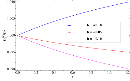
Figure 8: The GW luminosity distance $D_{\text{L}}^{\text{gw}}$ of meVSL. a) The ratio $D_{\text{L}}^{\text{gw}}/D_{\text{L}}$ for different values of $b$. b) The relative difference $\Delta D_{\text{L}}^{\text{gw}}/D_{\text{L}}(\%)$ between meVSL and GR for different values of $b$.

There have been similar results on the luminosity distance of GW for the modified gravity models [195, 196, 197, 198, 199]. It uses the fact that the time variation of the gravitational constant G can be constrained from the GW observations of merging binary neutron stars. One can relate the luminosity distance to the gravitational constant G from the Friedmann equation. This equally means that the GWs give information about the value of G at the time of the merger. Thus, the measured masses of neutron stars from the GW observations can be inconsistent with the theoretically allowed range, if there exists a significant time evolution of $G$ from the merging epoch to the present epoch. One might be able to place bounds on the variation of $G$ between the merger epoch and the present epoch by using GWs.

In meVSL, the ratio $D_{\text{L}}^{\text{gw}}/D_{\text{L}}$ is given by $(1+z)^{b/8}$ as given in Eq. (6.57). We plot this ratio in the left panel of Fig. 8. For a positive value of $b$, this ratio is greater than $1$. This ratio becomes less than 1 for the negative value of $b$. The solid, dashed, and, dot-dashed lines correspond $b=+0.1$, $-0.05$, and $-0.1$, respectively. We show the relative difference $\Delta D_{\text{L}}/D_{\text{L}}(\%)=(D_{\text{L}}^{\text{gw}}-D_{\text{L}})/D_{\text{L}}\times 100$ for different models (i.e., for different values of $b$) in the right panel of Fig. 8. For standard sirens, we need to compare the GW luminosity distance of meVSL to that of GR. There is about 1% at $z=1.2$ difference between two models when $|b|=0.1$. For values of $b$ smaller than $0.1$, there will be a sub-percent difference between two luminosity distances.

6.7 Hubble parameter

As we show in the subsection 5.1, the Hubble parameter of meVSL in Eq. (5.19) can be rewritten as

$$H(z) =H_{0}E(z)^{(\text{GR})}\left(1+z\right)^{-\frac{b}{4}}\equiv 100\,h(z)\,E(z)^{(\text{GR})}\,[\text{km/s/Mpc}]\,,$$ (6.59)

where $h[z]\equiv h(1+z)^{-b/4}$ with $h$ is known as 0.6688 in Planck 2018 [248]. Thus, the $h$-value is a constant in GR, but it can be interpreted as $h[z]$ cosmologically evolves in meVSL.

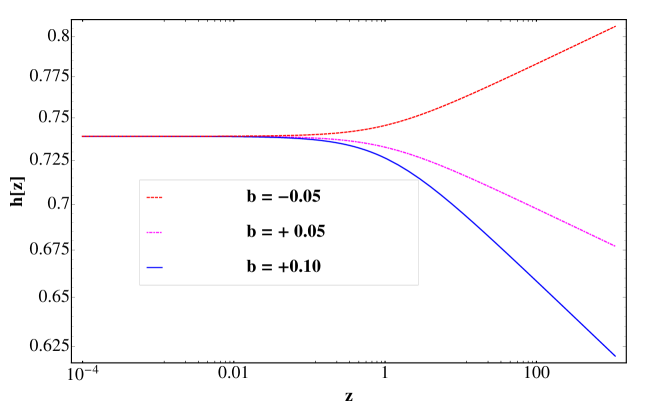
Figure 9: The cosmological evolution of the reduced Hubble parameters, $h[z]$ for the different values of $b$.

The present values of local measurements of the Hubble parameter, from the Cepheid-calibrated SNe [252, 253, 254, 255] and time delays of strong lensing [256, 257, 258], are close to 74 km/s/Mpc. However, $H_{0}$-values inferred from a $\Lambda$CDM fit to the CMB [248], various large-scale structures [259, 260, 261, 262, 263, 264, 265], and the local measurements based on the inverse distance ladder method [266] converge to 68 km/s/Mpc. This discrepancy (the so-called “Hubble tension” or “$H_{0}$-tension”) is not easily explained by any obvious systematic effect in either measurement [267, 268, 269, 270, 271, 272, 273], and so increasing attention is focusing on the possibility that this “Hubble tension” may be indicating new physics beyond the standard cosmological model [274, 275, 276, 277, 278].

If one adopts the $H_{0}$-tension as the evidence for the new physics, then there are two promising ways to alter early cosmology so that the tension between CMB-inferred value and the measured value of $H_{0}$ is reduced. These are either changing the early time expansion history or changing the details of recombination. The second effect is changes in the details of nucleosynthesis can be captured by changes in the primordial Helium mass fraction, parametrized by $Y_{\text{P}}^{(\text{BBN})}$. However, this is not the case for meVSL. Instead the expansion history can be modified in the early Universe in meVSL and this can be used to solve the $H_{0}$-tension.

We can interpret $h[z]=h(1+z)^{-b/4}$ in Eq. (6.59) as follows. Even though the present value of $h[z]$ is $h$, its past value was smaller (larger) than that of $h$ for the positive (negative) value of b. This is depicted in Fig. 9. The dashed, dot-dashed, and solid lines correspond $b=-0.05,0.05$, and $0.1$, respectively. If we choose $h=0.739$, then $h[z=1091]=0.6688$ when $b=0.057$. This can explain that the local measurement $0.74$ is identical to the CMB measured value, $0.67$.

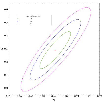
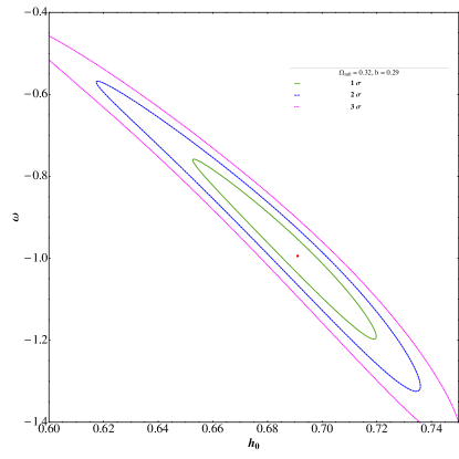
Figure 10: Contour plots of $h$ for $b$ and $\omega$. a) 1,2, and, 3-$\sigma$ contour plots for $h_{0}$ and $b$. b) 1,2, and, 3-$\sigma$ contour plots for $h_{0}$ and $\omega$.

The Hubble parameter which directly probes the expansion history of the Universe is also related to the differential redshift as, $H(z)=−(dz/dt)/(1+z)$, where $dz$ is obtained from the spectroscopic surveys and so a measurement of $dt$ provides the Hubble parameter. In fact, two methods are generally used to measure the Hubble parameter values H(z) at certain redshift and are extraction of H(z) from line-of-sight BAO data and differential age (DA) method estimating $H(z)$. We use 57 data points from the reference [279] out of which 31 data points measured with the DA method and 26 data points are obtained with BAO and other methods. We perform the maximum likelihood analysis to obtain the best fit values of $b$, $\omega$, and $h$ of meVSL by using these data. The best fit values of ($b,\omega,h$) = (0.290, -0.994, 0.691) if we adopt $\Omega_{m0}=0.32$ and $\Omega_{\Lambda 0}=0.68$. We obtain the 1, 2, and 3-$\sigma$ contour plots for the fixed $b$ and $\omega$, respectively. These are shown in figure 10. In the left panel of Fig. 10, the solid, dotted, and dashed lines correspond 1, 2, and, 3-$\sigma$ level contour plots with $\omega=-0.99$. In the right panel of Fig. 10, we also show the contour plots of $h$ verse $\omega$ for the fixed value of $b=0.29$. The solid, dotted, and dashed lines correspond 1, 2, and, 3-$\sigma$ level contour plots. In this case, the $h$-value can include both the local and the CMB values.

6.8 Strong lensing

In GR, the presence of matter curves spacetime, and this causes the deflection of the path of a light ray as a result. This process is known as the gravitational lensing. The most extreme bending of light (i.e., strong lensing) occurs when the lens is very massive and the source of the lens is close enough to it. In this case, lights can reach the observer through different paths and there can be more than one image of the source. One can estimate the volume of space back to the sources by using the number of discovered lenses. This volume depends strongly both on cosmological parameters and on gravity theories. However, there can be time delays for the changes in the images because the traveling distance for each image is different from each other due to the bending of space. One can estimate the present value of the Hubble constant, $H_{0}$ by using these time delays. In some cases, the source and the lens are in the special alignment to make light will be deflected to the observer and produce an Einstein ring. The Einstein radius, $\theta_{\text{E}}$ under the singular isothermal sphere (SIS) model is given by [99]

$$\theta_{\text{E}}=4\pi\frac{D_{A}^{\text{ls}}}{D_{A}^{\text{so}}}\frac{\sigma_{\text{SIS}}^{2}}{\tilde{c}^{2}}=4\pi\frac{D_{A}^{\text{ls}}}{D_{A}^{\text{so}}}\frac{\sigma_{\text{SIS}}^{2}}{\tilde{c}_{0}^{2}}(1+z)^{\frac{b}{2}}=\theta_{\text{E}}^{(\text{GR})}(1+z)^{\frac{b}{2}}\,,$$ (6.61)

where $D_{A}^{\text{ls}}$ is the angular diameter distance from the lens to the source, $D_{A}^{\text{so}}$ is that from the source to the observer, and $\sigma_{\text{SIS}}$ is the velocity dispersion due to the lens mass distribution. Angular diameter distances both in GR and in meVSL are same and only difference between two models is the speed of light in Eq. (6.61). $\theta_{\text{E}}$ is the observed quantity and one can estimate cosmological parameters from the angular diameters based on the given gravity theory. Thus, if meVSL is the true gravity theory governing our Universe, then one needs to insert $(1+z)^{b/2}$ into the Einstein radius obtained from GR in order to properly extract cosmological parameters from the strong lensing signal.

The observations of gravitationally lensed quasars are best understood in light of Fermat’s principle. Intervening mass between a source and an observer introduces an effective index of refraction, thereby increasing the light travel time. The competition between this Shapiro delay due to the gravitational field and the geometric delay from bending the ray paths leads to the formation of multiple images at the stationary points of the travel time [280].There exists a thin-lens approximation that applies when the optics are small compared to the distances to the source and the observer. In this approximation, we need only the effective potential, $\psi(\vec{x})=(2/\tilde{c}^{2})D_{\text{ls}}/D_{\text{s}}\int dz\phi$ found by integrating the 3D potential $\phi$ along the line of sight. The light-travel time is

$$\tau(\vec{x})=\frac{1+z_{\text{l}}}{\tilde{c}}\frac{D_{\text{l}}D_{\text{s}}}{D_{\text{ls}}}\left(\frac{1}{2}\left(\vec{x}-\vec{\beta}\right)^{2}-\psi(\vec{x})\right)=\tau^{(\text{GR})}(1+z)^{-\frac{b}{4}}\,,$$ (6.62)

where $\vec{x}$ is the angular position of the image, $\vec{\beta}$ is the angular position of the source, $\psi(\vec{x})$ is the effective potential, $z_{\text{l}}$ is the lens redshift. $D_{\text{l}}$, $D_{\text{s}}$, and $D_{\text{ls}}$ are angular diameter distances to the lens, to the source, and from the lens to the source, respectively. $\left(\vec{x}-\vec{\beta}\right)^{2}/2$ is the geometric delay in the small-angle approximation. Similar to the Einstein radius, one has the additional factor $(1+z)^{-b/4}$ in the light-travel time.

6.9 Fine structure constant

The strength of the electromagnetic interaction between elementary charged particles can be characterized by the so called the fine structure constant, $\alpha$ also known as Sommerfeld’s constant. This is a dimensionless constant obtained from the combination of other physical constant as

$$\alpha\equiv\frac{e^{2}}{4\pi\tilde{\epsilon}\hbar\tilde{c}}=\frac{e_{0}^{2}}{4\pi\tilde{\epsilon}_{0}\hbar_{0}\tilde{c}_{0}}(1+z)^{\frac{b}{4}}\equiv\alpha^{(\text{GR})}(1+z)^{\frac{b}{4}}\,,$$ (6.63)

where we use $e=e_{0}a^{-b/4}$, $\tilde{\epsilon}=\tilde{\epsilon}_{0}a^{-b/4}$, $\hbar=\hbar_{0}a^{-b/4}$, and $\tilde{c}=\tilde{c}_{0}a^{b/4}$ as shown both in Sec. 3.3 and in Sec. 3.4. In meVSL, we assume the conservation of the particle numbers and the above Eq. (6.63) is the consequence of this assumption. Compared to the $\alpha^{(\text{GR})}$, it has the additional factor, $(1+z)^{b/4}$ and thus $\alpha$ of meVSL in the past is larger (smaller) than $\alpha^{(\text{GR})}$ for the positive (negative) value of b. Thus, a temporal variation of $\alpha$ over cosmological time periods, $\dot{\alpha}/\alpha$ and the fractional difference of it $\Delta\alpha/\alpha_{0}$ are given by

$$\frac{\dot{\alpha}}{\alpha} =-\frac{b}{4}H(z)=-\frac{b}{4}(1+z)^{-\frac{b}{4}}H^{(\text{GR})}(z)\,,$$ (6.64)

$$\frac{\Delta\alpha}{\alpha_{0}} \equiv\frac{\alpha(z)-\alpha_{0}}{\alpha_{0}}=(1+z)^{\frac{b}{4}}-1\,,$$ (6.65)

where $\alpha_{0}=\alpha^{(\text{GR})}\approx 1/137$ denotes the value of $\alpha$ at the present epoch (i.e., $z=0$). Observational limits on these values from the Keck telescopes are $\dot{\alpha}/\alpha=(6.45\pm 1.35)\times 10^{-16}\text{yr}^{-1}$ and $\Delta\alpha/\alpha=(-5.43\pm 0.116)\times 10^{-6}$ for $0.2<z<3.7$ [281] . In order to satisfy these results, $b$ should be negative and its magnitude is about $10^{-5}$. This is a strong constrain on $b$ and if this value is adopted, then there might not be any observation that can be detected in cosmology.

The method to obtain these observational values of $\Delta\alpha$ is called as “Many Multiplet (MM)” method [73]. This method compares the relative velocity spacing between different metal ion transitions and relates it to possible variation in $\alpha$. For example, considering just a single transition, variation in $\alpha$ is related to the velocity shift $\Delta v_{i}$ of a transition

$$\frac{\Delta\alpha}{\alpha}\equiv\frac{\alpha_{\text{obs}}-\alpha_{\text{lab}}}{\alpha_{\text{lab}}}\approx-\frac{\Delta v_{i}}{2\tilde{c}}\frac{\omega_{i}}{q_{i}}=-\frac{\Delta v_{i}}{2\tilde{c}_{0}}\frac{\omega_{i}}{q_{i}}(1+z)^{\frac{b}{4}}\,,$$ (6.66)

where $q_{i}$ is the sensitivity of the transition to $\alpha$ variation, calculated from many-body relativistic corrections to the energy levels of ions and $\omega_{i}$ is its wavenumber measured in the laboratory. Thus, one should include the effect of the variation of the speed of light in the data analysis as given in the above Eq. (6.66). However, this effect is negligible and it might not affect the observational results.

6.10 The gravitational constant and the speed of light

The stringent limitations on any violation of the equivalence principle (EP) can be obtained from LLR. One can increase the accuracy of the limit on violation of the EP by change the laser ranges to the Moon. These analyses give an EP test. In addition to the SEP constraint, the PPN parameters $\gamma$ and $\beta$ affect the orbit of relativistic point masses, and $\gamma$ also influences time delay. LLR can test this orbital $\beta$ and $\gamma$ dependence, as well as geodesic de-Sitter precession, and $\dot{G}/G$. In this LLR analysis, the limit on the temporal variation of the gravitational constant is $\dot{G}/G=(4\pm 9)\times 10^{-13}\text{yr}^{-1}$ and $\dot{\tilde{c}}/\tilde{c}=(0\pm 2)\times 10^{-12}\text{yr}^{-1}$ [114].

One can use Eq. (5.15) to obtain the expressions of time variations of those quantities

$$\frac{\dot{G}}{G} =\frac{d\ln G}{dt}=bH=bH^{(\text{GR})}(1+z)^{-b}\,,$$ (6.67)

$$\frac{\dot{\tilde{c}}}{\tilde{c}} =\frac{d\ln\tilde{c}}{dt}=\frac{b}{4}H=\frac{b}{4}H^{(\text{GR})}(1+z)^{-\frac{b}{4}}\,.$$ (6.68)

We show these results in subection 5.1.

7 Conclusions

One of the main motivations for probing previous time-varying speed of light models is to provide alternative solutions for early time problems of the Big Bang model. However, we have investigated the new kind of time-varying speed of light model as an alternative solution for various late time problems of the standard $\Lambda$CDM model.

We have proposed the new time-varying speed of light model which satisfies the Lorentz invariance, including Maxwell’s equations and the local thermal equilibrium. The cosmological evolution of the speed of light also induces the evolutions of both permittivity and permeability. As a consequence, the charge also cosmologically evolves to satisfy the charge conservation. One can also obtain the cosmological evolution of the Planck constant from the conservation of the number density by using the local thermal equilibrium. This also provides the cosmological evolution of frequency. However, the Boltzmann constant is still constant, and both the wavelength and the temperature are the same as those of GR. The conservation of number density also provides the cosmological evolution of the rest mass. When we derive the Einstein field equation from the action with allowing the time variation of the speed of light, this also induces the time evolution of the gravitational constant, $G$. All of these consequences are summarized in table 1, and we dubbed this new varying speed of light model as the “minimally extended varying speed of light” (meVSL).

In table 2, we have summarized both the consequent time variations of other physical constants and modifications of some observable quantities derived in this manuscript.

All of these changes in both the physical constants and the physical quantities induce the modifications of the Friedmann equations when we apply the meVSL to the Friedmann-Lemaître-Robertson-Walker metric. Both the expansion speed (i.e., the Hubble parameter) and the expansion acceleration are modified in meVSL model compared to those of GR. However, the gravitational redshift is still the same as that of GR, and the geometrical distances including transverse comoving distance and the angular diameter distance are also not changed in the meVSL model. But the luminosity distance is modified due to the modification of the cosmological evolution of the frequency. meVSL also affects the cosmological observations, like the cosmic microwave background, the Sunyaev-Zel^’dovich effect, the baryon acoustic oscillation, the supernovae, the gravitational waves, the Hubble parameter, and the strong gravitational lensing.

Thus, it is necessary to include the effect of the time variation of the speed of light when one investigates cosmological observations. This will induce changes in cosmological parameter values compared to those obtained from GR. As an example, we have scrutinized the Hubble tension, and meVSL might be able to solve this problem as we have shown in section 6.7. One can analyze the cosmological observations based on meVSL to obtain new best fit values on cosmological parameters.

Table 2: Both equalities and differences of physical observables between meVSL and GR. EM, TD, and KN denote electromagnetism, thermodynamics, and kinematics, respectively.

Criteria		Equality	Difference
SR	EM	wavelegth $\lambda$	electric charge $e=e_{0}a^{-\frac{b}{4}}$ frequency $\nu=\nu_{0}a^{\frac{b}{4}}$
	TD	Boltzmann constant $k_{B}$ temperature $T$	Planck constant $h=h_{0}a^{-\frac{b}{4}}$
GR	KN	redshift $z$	gravitational constant $G=G_{0}a^{b}$
	FLRW	equation of state $\omega$ Hubble radius $c/H$ angular distance $D_{A}$	mass density $\rho=\rho^{(\text{GR})}a^{-\frac{b}{2}}$ Hubble parameter $H=H^{(\text{GR})}a^{\frac{b}{4}}$ luminosity distance $D_{L}=D_{L}^{(\text{GR})}a^{\frac{b}{8}}$

Appendix A Appendix

In the appendix, we show some detailed calculations in contents.

Appendix B Special Relativity

B.1 Four acceleration

A point in Minkowski spacetime is a time and spatial position called an event, or sometimes the four-position, described in some reference frame by a set of four coordinates

$$x^{\mu}=\left(c\left(a\right)t\,,x^{i}(t)\right)=\left(c\left(a\right)\tau\,,0\right)\;,$$ (B.1)

where $x^{i}$ is the three-dimensional space position vector which is a function of the coordinate time, $t$ in the same frame. These coordinates are the components of the position four-vector for the event. In the SR, the four-positions are four-vectors that transform one inertial frame of reference to another by Lorentz transformations. A clock fastened to a particle moving along a world-line in four-dimensional spacetime measures the particle’s proper time $\tau$. This relation is shown in the second equality of Eq. (B.1). The four-velocity of a particle is defined as the rate of change of its four-position with respect to proper time and is the tangent vector to the particle’s world line

$$U^{\mu}\equiv\frac{dx^{\mu}}{d\tau}=\frac{dt}{d\tau}\left(\tilde{c}\,,v^{i}\right)\equiv\gamma\left(\tilde{c}\,,v^{i}\right)\equiv\left(\tilde{\tilde{c}}\,,0\right)\quad,\quad\text{where}\;,$$

$$\tilde{c}\equiv\left(\frac{d\ln c}{d\ln a}Ht+1\right)c\quad\text{and}\quad\tilde{\tilde{c}}\equiv\left(\gamma\frac{d\ln c}{d\ln a}H\tau+1\right)c\,,$$ (B.2)

where the Lorentz factor, $\gamma$ represents the time dilation of a process due to the fact that it takes a proper time $\Delta\tau$ in its own rest frame has a longer duration $\Delta t$ measured by another observer moving relative to the rest frame. The $Ht$-term in the above Eq. (B.2) can be obtained in the FLRW universe as

$$E^{2}=H^{2}/H_{0}^{2}=\sum_{i}\Omega_{0i}a^{-3(1+\omega_{i})+b/2}\,\,\Rightarrow\,\,E(z)=(1+z)^{-b/4}\sqrt{\sum_{i}\Omega_{i0}(1+z)^{3(1+\omega_{i})}}\;,$$ (B.3)

$$H_{0}\int_{0}^{t}dt^{\prime}=H_{0}t=-\int_{\infty}^{z}\frac{dz^{\prime}}{(1+z^{\prime})E(z^{\prime})}=\int_{z}^{\infty}\frac{dz^{\prime}}{(1+z^{\prime})^{1-b/4}\sqrt{\sum_{i}\Omega_{i0}(1+z^{\prime})^{3(1+\omega_{i})}}}\;,$$ (B.4)

$$Ht=H_{0}tE=(1+z)^{-b/4}\sqrt{\sum_{i}\Omega_{i0}(1+z)^{3(1+\omega_{i})}}\int_{z}^{\infty}\frac{dz^{\prime}}{(1+z^{\prime})^{1-b/4}\sqrt{\sum_{i}\Omega_{i0}(1+z^{\prime})^{3(1+\omega_{i})}}}\;.$$ (B.5)

$H_{0}t_{0}\sim 1$ and thus if $c$ varies as a function of the scale factor $a$ then $\tilde{c}_{0}$ is different from $c_{0}$ as shown in Eq. (B.2). We emphasize that the value of $\tilde{c}$ is a constant at the given hypersurface (for the given cosmic time). The four-acceleration, $A^{\mu}$ is defined as the rate of change in four-velocity with respect to the particle’s proper time along its worldline

$$A^{\mu} \equiv\frac{dU^{\mu}}{d\tau}=\frac{dt}{d\tau}\frac{dU^{\mu}}{dt}=\gamma\left[\dot{\gamma}\left(\,\tilde{c},v^{i}\,\right)+\gamma\left(\,\dot{\tilde{c}},a^{i}\,\right)\right]=\gamma^{2}\left[\frac{\dot{\gamma}}{\gamma}\left(\,\tilde{c},v^{i}\,\right)+\left(\,\dot{\tilde{c}},a^{i}\,\right)\right]\,,$$ (B.6)

where we use Eq. (B.2) and dots denote the derivatives with respect to the coordinate time, $t$. We explicitly write terms in the above equation (B.6)

$$\dot{\tilde{c}} =\frac{b}{4}H\tilde{c}\quad,\quad\frac{\dot{\breve{r}}}{\breve{r}}=\left(\frac{\dot{\tilde{\tilde{c}}}}{\tilde{\tilde{c}}}-\frac{\dot{\tilde{c}}}{\tilde{c}}\right)\quad,\quad\frac{\dot{\tilde{\gamma}}}{\tilde{\gamma}}=\tilde{\gamma}^{2}\left(\frac{\vec{v}\cdot\vec{a}}{\tilde{c}^{2}}-\frac{v^{2}}{\tilde{c}^{2}}\frac{\dot{\tilde{c}}}{\tilde{c}}\right)\,,$$ (B.7)

$$\frac{\dot{\gamma}}{\gamma} =\frac{\dot{\breve{r}}}{\breve{r}}+\frac{\dot{\tilde{\gamma}}}{\tilde{\gamma}}=\left(\frac{\dot{\tilde{\tilde{c}}}}{\tilde{\tilde{c}}}-\frac{\dot{\tilde{c}}}{\tilde{c}}\right)+\tilde{\gamma}^{2}\left(\frac{\vec{v}\cdot\vec{a}}{\tilde{c}^{2}}-\frac{v^{2}}{\tilde{c}^{2}}\frac{\dot{\tilde{c}}}{\tilde{c}}\right)\,,$$ (B.8)

where we use the explicit form of $\tilde{c}$ given in Eq. (5.15) to have

$$\frac{\dot{\tilde{c}}}{\tilde{c}}=\frac{d\ln\tilde{c}}{dt}=\frac{d\ln a}{dt}\frac{d\ln\tilde{c}}{d\ln a}=\frac{b}{4}H\,.$$ (B.9)

We inserts Eqs. (B.7) and (B.8) into Eq. (B.6) to obtain

$$A^{\mu} =\left(\gamma\dot{\gamma}\tilde{c}+\gamma^{2}\dot{\tilde{c}}\,,\gamma\dot{\gamma}\vec{v}+\gamma^{2}\vec{a}\right)=\gamma^{2}\left[\left[\left(\frac{\dot{\tilde{\tilde{c}}}}{\tilde{\tilde{c}}}-\frac{\dot{\tilde{c}}}{\tilde{c}}\right)+\tilde{\gamma}^{2}\left(\frac{\vec{v}\cdot\vec{a}}{\tilde{c}^{2}}-\frac{v^{2}}{\tilde{c}^{2}}\frac{\dot{\tilde{c}}}{\tilde{c}}\right)\right]\left(\,\tilde{c},\vec{v}\,\right)+\left(\,\dot{\tilde{c}},\vec{a}\,\right)\right]$$

$$=\gamma^{2}\tilde{\gamma}^{2}\left(\frac{\vec{v}\cdot\vec{a}}{\tilde{c}}-\beta^{2}\dot{\tilde{c}}+\tilde{\gamma}^{-2}\frac{\dot{\tilde{\tilde{c}}}}{\tilde{\tilde{c}}}\tilde{c}\,,\frac{\vec{v}\times\left(\vec{v}+\vec{a}\right)}{\tilde{c}^{2}}+\tilde{\gamma}^{-2}\frac{\dot{\tilde{\tilde{c}}}}{\tilde{\tilde{c}}}\vec{v}-\frac{\dot{\tilde{c}}}{\tilde{c}}\vec{v}+\vec{a}\right)\,,$$ (B.10)

where we use

$$\vec{v}\left(\vec{v}\cdot\vec{a}\right)=\vec{v}\times\left(\vec{v}\times\vec{a}\right)+v^{2}\vec{a}\quad,\quad\frac{v^{2}}{\tilde{c}^{2}}+\tilde{\gamma}^{-2}=1\,.$$ (B.11)

Even though we express the four-acceleration in Eq. (B.10) by including $\dot{\tilde{c}}$ and $\dot{\tilde{\tilde{c}}}$ terms, we should drop these terms from the expression in order to properly describe $A^{\mu}$ as a local quantity in the constant time hypersurface. And $\tilde{c}=\tilde{\tilde{c}}$ in this frame. Thus, the four-acceleration is simply expressed by

$$A^{\mu} =\gamma^{2}\tilde{\gamma}^{2}\left(\frac{\vec{v}\cdot\vec{a}}{\tilde{c}}-\beta^{2}\dot{\tilde{c}}+\tilde{\gamma}^{-2}\frac{\dot{\tilde{\tilde{c}}}}{\tilde{\tilde{c}}}\tilde{c}\,,\frac{\vec{v}\times\left(\vec{v}+\vec{a}\right)}{\tilde{c}^{2}}+\vec{a}\right)\,.$$ (B.12)

This is the same as the four-acceleration of SR if $\tilde{c}=c$ and thus $\tilde{\gamma}=\gamma$. The scalar product of a particle’s four-velocity and its four-acceleration $U^{\mu}A_{\mu}$ is given by

$$U^{\mu}A_{\mu} =\gamma^{3}\tilde{\gamma}^{2}\left(-\vec{v}\cdot\vec{a}+\frac{\dot{\tilde{c}}}{\tilde{c}}v^{2}-\tilde{\gamma}^{-2}\frac{\dot{\tilde{\tilde{c}}}}{\tilde{\tilde{c}}}\tilde{c}^{2}+\vec{v}\cdot\vec{a}+\frac{\vec{v}\times\left(\vec{v}\times\vec{a}\right)}{\tilde{c}^{2}}\cdot\vec{v}-\frac{\dot{\tilde{c}}}{\tilde{c}}v^{2}+\tilde{\gamma}^{-2}\frac{\dot{\tilde{\tilde{c}}}}{\tilde{\tilde{c}}}v^{2}\right)$$

$$=-\gamma^{3}\tilde{\gamma}^{2}\tilde{\gamma}^{-2}\frac{\dot{\tilde{\tilde{c}}}}{\tilde{\tilde{c}}}\tilde{c}^{2}\left(1-\frac{v^{2}}{\tilde{c}^{2}}\right)=-\gamma^{3}\tilde{\gamma}^{-2}\frac{\dot{\tilde{\tilde{c}}}}{\tilde{\tilde{c}}}\tilde{c}^{2}=-\tilde{\tilde{c}}\frac{d\tilde{\tilde{c}}}{d\tau}\,.$$ (B.13)

Again, in the local reference frame, one obtains constant $\tilde{c}$ and $\tilde{\tilde{c}}$ and thus the inner product between the four-velocity and the four-acceleration becomes zero.

B.2 Electromagnetism

In this appendix, we review Maxwell’s equations in 4-dimensional spacetime. The electromagnetic field is fully described by a four-potential $A^{\mu}$

$$A^{\mu}=\left(\frac{\phi}{\tilde{c}}\,,A^{i}\right)\;,$$ (B.14)

where $\phi$ is the electrostatic scalar potential and $A^{i}$ is the vector potential. The Lagrangian of a charged particle and an electromagnetic field is given by

$$L_{\text{EM}} \equiv\int\mathcal{L}d^{3}x=-\int\rho_{m}\tilde{c}\sqrt{U_{\alpha}U^{\alpha}}d^{3}x-\int\frac{1}{4\tilde{\mu}}F_{\alpha\beta}F^{\alpha\beta}d^{3}x+\int j_{\alpha}A^{\alpha}d^{3}x\,,$$ (B.15)

$$=-\frac{1}{2}m_{\text{rs}}U^{\alpha}U_{\alpha}-\int\left(\frac{1}{4\tilde{\mu}}F_{\alpha\beta}F^{\alpha\beta}-j_{\alpha}A^{\alpha}\right)d^{3}x\,,$$ (B.16)

$$F_{\alpha\beta}F^{\alpha\beta} =\left(\partial_{\alpha}A_{\beta}-\partial_{\beta}A_{\alpha}\right)\left(\partial^{\alpha}A^{\beta}-\partial^{\beta}A^{\alpha}\right)=2\left(\partial_{\alpha}A_{\beta}\partial^{\alpha}A^{\beta}-\partial_{\beta}A_{\alpha}\partial^{\alpha}A^{\beta}\right)\,,$$ (B.17)

$$=2\left(g_{\alpha\delta}g_{\beta\epsilon}\partial^{\delta}A^{\epsilon}\partial^{\alpha}A^{\beta}-g_{\alpha\delta}g_{\beta\epsilon}\partial^{\epsilon}A^{\delta}\partial^{\alpha}A^{\beta}\right)\,,$$

where $m_{\text{rs}}$ is the rest mass of a charged particle, $F^{\alpha\beta}$ is the electromagnetic field strength tensor, a four-current density $j^{\alpha}=\rho_{\text{EM}}^{\text{rs}}U^{\alpha}=\rho_{\text{EM}}^{\text{rs}}\gamma\left(\tilde{c}\,,\vec{v}\right)$, and the rest charge density $\rho_{\text{EM}}^{\text{rs}}=q^{\text{rs}}\delta(\vec{r}-\vec{s})$. Thus, the action of the electromagnetic field is given by

$$S_{\text{EM}}=\int L_{\text{EM}}d\tau=\int L_{\text{EM}}\gamma^{-1}dt\,.$$ (B.18)

The Euler-Lagrange equations for the electromagnetic field provide

$$\frac{\partial\mathcal{L}}{\partial A^{\nu}}=j_{\alpha}\frac{\partial A^{\alpha}}{\partial A^{\nu}}=j_{\alpha}\delta^{\alpha}_{\nu}=j_{\nu}\quad,\quad\frac{\partial\mathcal{L}}{\partial(\partial^{\mu}A^{\nu})}=\frac{\partial}{\partial(\partial^{\mu}A^{\nu})}\left(-\frac{1}{4\tilde{\mu}}F_{\alpha\beta}F^{\alpha\beta}\right)\quad,\quad\frac{\partial\left(F_{\alpha\beta}F^{\alpha\beta}\right)}{\partial(\partial^{\mu}A^{\nu})}=4F_{\mu\nu}\,,$$

$$\partial^{\mu}\frac{\partial\mathcal{L}}{\partial(\partial^{\mu}A^{\nu})}=\partial^{\mu}\left(-\frac{F_{\mu\nu}}{\tilde{\mu}}\right)=-\frac{1}{\tilde{\mu}}\partial^{\mu}F_{\mu\nu}+\frac{\partial^{\mu}\tilde{\mu}}{\tilde{\mu}^{2}}F_{\mu\nu}\,,$$

$$\partial^{\alpha}F_{\alpha\beta}=-\tilde{\mu}j_{\beta}+\frac{\partial^{\alpha}\tilde{\mu}}{\tilde{\mu}}F_{\alpha\beta}=-\tilde{\mu}j_{\beta}+\left(\partial^{\alpha}\ln\tilde{\mu}\right)F_{\alpha\beta}\,,$$ (B.19)

$$\epsilon^{\alpha\beta\gamma\delta}\partial_{\gamma}F_{\alpha\beta}=0\,,$$ (B.20)

where $\tilde{\mu}$ is the permeability and $\epsilon_{\alpha\beta\gamma\delta}$ is a four-dimensional Levi-Civita symbol. Since $\tilde{c}$ varies as a function of the scale factor in meVSL, it is reasonable to assume that so does $\tilde{\mu}$. Thus, we write the permeability in the meVSL as $\tilde{\mu}[a]$ and the modification in Eq. (B.19) does not contribute to Maxwell’s equation in the local inertial frame. Eq. (B.19) includes inhomogeneous Maxwell’s equations (Gauss’s law and Ampère’s law) and Eq. (B.20) implies Bianchi’s identity (Gauss’s law for magnetism and Maxwell-Faraday equation). We can explicitly rewrite the above equations as

$$F_{0i}=\partial_{0}A_{i}-\partial_{i}A_{0}=\frac{1}{\tilde{c}}\left(\frac{dA_{i}}{dt}+\frac{d\phi}{dx^{i}}\right)\quad,\quad J^{\alpha}=\left(\rho_{\text{EM}}\tilde{c}\,,\vec{j}\right)\,,$$ (B.21)

where $\rho_{\text{EM}}$ is the charge density and $\vec{j}$ is the conventional current density.

We adopt the electric field $E_{i}=-\tilde{c}F_{0i}$ and the magnetic field $B_{i}=1/2\epsilon_{ijk}F^{jk}$ to obtain

$$\partial^{i}F_{i0}=-\tilde{\mu}j_{0}+\left(\partial^{i}\ln\tilde{\mu}\right)F_{i0}\quad,\quad\beta=0$$

$$\partial^{i}\frac{1}{\tilde{c}}E_{i}(t)=-\tilde{\mu}j_{0}(t)+\left(\partial^{i}\ln\tilde{\mu}\right)\frac{1}{\tilde{c}}E_{i}(t)\quad\Longrightarrow\quad\vec{\nabla}\cdot\vec{E}(t)=-\tilde{\mu}\tilde{c}j_{0}(t)=\rho\tilde{\mu}\tilde{c}^{2}=\frac{\rho(t)}{\tilde{\epsilon}}\,,$$ (B.22)

where we use the fact that $\tilde{\mu}[a]$ is a function of the scale factor $a$ and thus $\tilde{c}[a]^{2}=1/(\tilde{\mu}[a]\tilde{\epsilon}[a])$. We obtain $\tilde{c}=\tilde{c}_{0}a^{b/4}$ and $\tilde{\epsilon}=\tilde{\epsilon}_{0}a^{-b/4}$ and $\tilde{\mu}=\tilde{\mu}_{0}a^{-b/4}$. Eq. (B.22) is the same as that of SR at the given cosmic epoch. We also obtain the Ampère’s law by taking $\beta$ for the spatial index,

$$\partial^{\alpha}F_{\alpha k}=-\mu j_{k}+\frac{\partial^{\alpha}\mu}{\mu}F_{\alpha k}\quad,\quad\beta=k$$

$$\partial^{0}F_{0k}+\partial^{i}F_{ik}=-\mu j_{k}+\frac{\partial^{0}\mu}{\mu}F_{0k}$$

$$\Longrightarrow\quad-\frac{1}{\tilde{c}^{2}}\frac{d\vec{E}(t)}{dt}+\vec{\nabla}\times\vec{B}=\tilde{\mu}\vec{j}(t)-\frac{d\ln[\tilde{c}\tilde{\mu}]}{dt}\frac{\vec{E}(t)}{\tilde{c}}=\tilde{\mu}\vec{j}(t)-\frac{d\ln[\tilde{c}_{0}\tilde{\mu}_{0}]}{dt}\frac{\vec{E}(t)}{\tilde{c}}=\tilde{\mu}\vec{j}\,.$$ (B.23)

Thus, Ampère’s law is the same as that of SR, too.

In SR, charge conservation is that the Lorentz invariant divergence of $J^{\alpha}$ is zero

$$\frac{\partial J^{\alpha}}{\partial x^{\alpha}}=\partial_{\alpha}J^{\alpha}=\frac{d}{\tilde{c}dt}\left(\rho\tilde{c}\right)+\vec{\nabla}\cdot\vec{j}=0\,,$$ (B.24)

Similarly, the continuity equation in GR with FLRW metric is written as

$$\nabla_{\alpha}J^{\alpha} =\partial_{\alpha}J^{\alpha}+\Gamma^{\alpha}_{\alpha\beta}J^{\beta}=0=\partial_{0}J^{0}+\partial_{i}J^{i}+\Gamma^{k}_{k0}J^{0}=\frac{d}{\tilde{c}dt}\left(\rho\tilde{c}\right)+\vec{\nabla}\cdot\vec{j}+3\frac{H}{\tilde{c}}\rho\tilde{c}\,.$$ (B.25)

The continuity equation can be solved

$$\frac{d\rho}{dt}+\frac{d\ln\tilde{c}}{dt}\rho+3\frac{d\ln a}{dt}\rho=-\vec{\nabla}\cdot\vec{j}$$

$$\frac{d\ln\rho}{dt}+3\frac{d\ln a}{dt}+\frac{d\ln\tilde{c}}{dt}=\frac{d\ln\rho}{dt}+\left(3+\frac{b}{4}\right)\frac{d\ln a}{dt}=0\quad\text{if}\quad\vec{j}=0$$

$$\rho_{\text{EM}}=\rho_{\text{EM}0}a^{-3-\frac{b}{4}}\,,$$ (B.26)

where $\rho_{\text{EM}0}$ denotes the present value of the charge density. Thus, Gauss’s law in Eq. (B.22) becomes

$$\nabla\cdot\vec{E}=\frac{\rho_{\text{EM}}}{\tilde{\epsilon}}=\frac{\rho_{\text{EM}0}a^{-b/4}}{\tilde{\epsilon}_{0}a^{-b/4}}=\frac{\rho_{\text{EM}0}}{\tilde{\epsilon}_{0}}\,.$$ (B.27)

This means that Gauss’s law holds for any epoch in meVSL.

B.3 Thermal Equilibrium

The perfect blackbody spectrum of the CMB is a piece of good observational evidence showing that the early universe was in local thermal equilibrium. The hot big bang model predicts thermal equilibrium above 100 GeV. To describe the subsequent evolution of the universe, we need to recall some basic facts of equilibrium thermodynamics, suitably generalized to apply to an expanding universe. It is convenient to describe the system of a weakly interacting particle in phase space, where it is described by the positions and momenta of all particles. In quantum mechanics, the momentum eigenstates of a particle included in a volume $V=L^{3}$ have a discrete spectrum. Then, the density of states in momentum space $\{{\bf p}\}$ is given by $L^{3}/h^{3}=V/h^{3}$, and the state density in phase space $\{{\bf x},{\bf p}\}$ is $h^{-3}$. If $g$ denotes the internal degrees of freedom (e.g. spin) of the particle, then the density of states becomes

$$\frac{g}{h^{3}}=\frac{g}{(2\pi\hbar)^{3}}\;.$$ (B.28)

The thermal equilibrium hypothesis is held until the nuclear interaction rate is not less than the expansion rate of the Universe. The distribution function is a function $f=f(\vec{x},\vec{p},t)$ of the position, of the proper momentum, and of the time. In other words, it is a function that takes its values in the phase space. It can be thought of as a probability density

$$f(t,\vec{x},\vec{p})\frac{d^{3}{\bf x}d^{3}{\bf p}}{\mathcal{N}}=f(t,p)\frac{d^{3}{\bf x}d^{3}{\bf p}}{\mathcal{N}}\;,$$ (B.29)

which is the probability of finding a particle at the given time $t$ in a small volume $d^{3}{\bf x}d^{3}{\bf p}$ of the phase space centered in $\{{\bf x},{\bf p}\}$, and $\mathcal{N}$ is some suitable normalization. We use the fact that distribution is homogeneous and isotropy to use $f(t,\vec{x},\vec{p})=f(t,p)$. In the early universe, the chemical potentials of all particles are so small that one can neglect them and thus the distribution functions are given by

$$f(p)=\frac{1}{\exp[E/(k_{\text{B}}T)]\pm 1}\,,$$ (B.30)

where $+$ sign and $-$ sign is for fermions and bosons, respectively. Because of the Heisenberg uncertainty principle of quantum mechanics, no particle can be localized in the phase space in a point $\{{\bf x},{\bf p}\}$, but at most in a small volume $\mathcal{N}=h^{3}$ about that point, where $h$ is Planck constant. Therefore, the probability density is given by

$$d\mathcal{P}(t,\vec{x},\vec{p})=f(t,p)\frac{d^{3}{\bf x}d^{3}{\bf p}}{(2\pi\hbar)^{3}}\;.$$ (B.31)

Integrating the distribution function with respect to the momentum, one gets the particle number density

$$n(t,\vec{x})\equiv g\int\frac{d^{3}{\bf p}}{(2\pi\hbar)^{3}}f(t,p)\;.$$ (B.32)

In general, one can write the energy-momentum tensor in terms of the distribution function as

$$T^{\mu}_{\nu}(t,x)=g\int\frac{dP_{1}dP_{2}dP_{3}}{(2\pi\hbar)^{3}}\frac{1}{\sqrt{-g}}\frac{cP^{\mu}P_{\nu}}{P^{0}}f(t,p)\;,$$ (B.33)

where $P^{\mu}=dx^{\mu}/d\lambda$ is the comoving momentum.

This equation satisfies the mass-shell condition. In order to use thermodynamics, one can calculate the number densities, energy densities, and the pressures of the relativistic and non-relativistic particles

$$n=\frac{g}{2\pi^{2}\hbar^{3}}\int_{0}^{\infty}dp\frac{p^{2}}{\exp[\sqrt{p^{2}c^{2}+m^{2}c^{4}}/k_{\text{B}}T]\pm 1}\,,$$ (B.34)

$$\rho\tilde{c}^{2}=\frac{g}{2\pi^{2}\hbar^{3}}\int_{0}^{\infty}dp\frac{p^{2}\sqrt{p^{2}c^{2}+m^{2}c^{4}}}{\exp[\sqrt{p^{2}c^{2}+m^{2}c^{4}}/k_{\text{B}}T]\pm 1}\,,$$ (B.35)

$$P=\frac{g}{2\pi^{2}\hbar^{3}}\int_{0}^{\infty}dp\frac{p^{4}c^{2}/\sqrt{p^{2}c^{2}+m^{2}c^{4}}}{3\left(\exp[\sqrt{p^{2}c^{2}+m^{2}c^{4}}/k_{\text{B}}T]\pm 1\right)}\,.$$ (B.36)

If we define $x\equiv\beta mc^{2}$, $\xi\equiv\beta pc$, and $\beta=1/(k_{\text{B}}T)$, then above equations are rewritten as

$$n=\frac{g}{2\pi^{2}}\left(\frac{k_{\text{B}}T}{\hbar c}\right)^{3}\int_{0}^{\infty}d\xi\frac{\xi^{2}}{\exp[\sqrt{\xi^{2}+x^{2}}]\pm 1}\equiv\frac{g}{2\pi^{2}}\left(\frac{k_{\text{B}}T}{\hbar c}\right)^{3}I_{\pm}(x)\,,$$ (B.37)

$$\rho\tilde{c}^{2}=\frac{g}{2\pi^{2}}\left(\frac{k_{\text{B}}^{4}T^{4}}{\hbar^{3}c^{3}}\right)\int_{0}^{\infty}d\xi\frac{\xi^{2}\sqrt{\xi^{2}+x^{2}}}{\exp[\sqrt{\xi^{2}+x^{2}}]\pm 1}\equiv\frac{g}{2\pi^{2}}\left(\frac{k_{\text{B}}^{4}T^{4}}{\hbar^{3}c^{3}}\right)J_{\pm}(x)\,,$$ (B.38)

$$P=\frac{g}{2\pi^{2}}\left(\frac{k_{\text{B}}^{4}T^{4}}{\hbar^{3}c^{3}}\right)\int_{0}^{\infty}d\xi\frac{\xi^{4}/\sqrt{\xi^{2}+x^{2}}}{3\left(\exp[\sqrt{\xi^{2}+x^{2}}]\pm 1\right)}\equiv\frac{g}{2\pi^{2}}\left(\frac{k_{\text{B}}^{4}T^{4}}{\hbar^{3}c^{3}}\right)K_{\pm}(x)\,.$$ (B.39)

Thus, the number densities, energy densities, and the pressures of relativistic and non-relativistic particles are given by

$$n =\begin{cases}\frac{g}{\pi^{2}}\left(\frac{k_{\text{B}}T}{\tilde{\hbar}\tilde{c}}\right)^{3}\frac{3}{4}\zeta(3)&\text{fermion}\\ \frac{g}{\pi^{2}}\left(\frac{k_{\text{B}}T}{\tilde{\hbar}\tilde{c}}\right)^{3}\zeta(3)&\text{boson}\\ g\left(\frac{1}{2\pi}\frac{m_{\text{rs}}\tilde{c}^{2}}{\tilde{\hbar}\tilde{c}}\frac{k_{\text{B}}T}{\tilde{\hbar}\tilde{c}}\right)^{\frac{3}{2}}e^{-\frac{m_{\text{rs}}\tilde{c}^{2}}{k_{\text{B}}T}}&\text{non-relativistic}\end{cases}\,,$$ (B.40)

$$\rho\tilde{c}^{2} =\begin{cases}\frac{g\pi^{2}}{30}\frac{\left(k_{\text{B}}T\right)^{4}}{\left(\tilde{\hbar}\tilde{c}\right)^{3}}\frac{7}{8}&\text{fermion}\\ \frac{g\pi^{2}}{30}\frac{\left(k_{\text{B}}T\right)^{4}}{\left(\tilde{\hbar}\tilde{c}\right)^{3}}&\text{boson}\\ n\left(m_{\text{rs}}\tilde{c}^{2}+\frac{3}{2}k_{\text{B}}T\right)\approx nm_{\text{rs}}\tilde{c}^{2}&\text{non-relativistic}\end{cases}\,,\quad P=\begin{cases}\frac{1}{3}\rho\tilde{c}^{2}&\text{fermion}\\ \frac{1}{3}\rho\tilde{c}^{2}&\text{boson}\\ nT\approx 0&\text{non-relativistic}\end{cases}\,.$$ (B.41)

B.4 Lorentz Transformation

From the translational symmetry of space and time, a transformation of the coordinates $x$ and $t$ from the inertial reference frame $\mathcal{O}$ to $x^{\prime}$ and $t^{\prime}$ in another reference frame $\mathcal{O}^{\prime}$ should be linear functions. This fact is written by

$$\begin{pmatrix}t^{\prime}\\ x^{\prime}\end{pmatrix}=\begin{pmatrix}A&B\\ C&D\end{pmatrix}\begin{pmatrix}t\\ x\end{pmatrix}\quad,\quad t^{\prime}=At+Bx\quad,\quad x^{\prime}=Ct+Dx\,.$$ (B.42)

If we set $x^{\prime}=0$ as the origin of $\mathcal{O}^{\prime}$ and it moves with velocity $v$ relative to $\mathcal{O}$, so that $x=vt$

$$x^{\prime} =Ct+Dx\Rightarrow 0=Ct+Dvt=(C+Dv)t\Rightarrow C=-vD\,,$$

$$x^{\prime} =D(-vt+x)\,.$$ (B.43)

Now $x=0$ is the origin of $\mathcal{O}$ and it moves with velocity $-v$ relative to $\mathcal{O}^{\prime}$, so that $x^{\prime}=-vt^{\prime}$

$$x^{\prime} =D(-vt+x)\Rightarrow-vt^{\prime}=-Dvt+0\Rightarrow t^{\prime}=Dt\,,$$

$$t^{\prime} =At+Bx\Rightarrow t^{\prime}=At+0\Rightarrow t^{\prime}=At\,,$$

$$A =D\,.$$ (B.44)

One can rewrite Eq. (B.42) as

$$t^{\prime} =At+Bx=A(t+Fx)\quad\text{where}\quad F=B/A\,.$$ (B.45)

If one changes the notation $A$ as $\gamma$, then the above equation (B.45) becomes

$$t^{\prime} =\gamma\left(t+Fx\right)\quad,\quad x^{\prime}=\gamma\left(-vt+x\right)\quad,\quad\begin{pmatrix}t^{\prime}\\ x^{\prime}\end{pmatrix}=\gamma[v]\begin{pmatrix}1&F[v]\\ -v&1\end{pmatrix}\begin{pmatrix}t\\ x\end{pmatrix}\,.$$ (B.46)

A Combination of two Lorentz transformations also must be a Lorentz transformation (form a group). If a reference frame $\mathcal{O}^{\prime}$ moving relative to $\mathcal{O}$ with velocity $v_{1}$ and a reference frame $\mathcal{O}^{\prime\prime}$ moving relative to $\mathcal{O}^{\prime}$ with velocity $v_{2}$ then

$$\begin{pmatrix}t^{\prime\prime}\\ x^{\prime\prime}\end{pmatrix} =\gamma[v_{2}]\begin{pmatrix}1&F[v_{2}]\\ -v_{2}&1\end{pmatrix}\begin{pmatrix}t^{\prime}\\ x^{\prime}\end{pmatrix}=\gamma[v_{2}]\begin{pmatrix}1&F[v_{2}]\\ -v_{2}&1\end{pmatrix}\gamma[v_{1}]\begin{pmatrix}1&F[v_{1}]\\ -v_{1}&1\end{pmatrix}\begin{pmatrix}t\\ x\end{pmatrix}$$

$$=\gamma[v_{2}]\gamma[v_{1}]\begin{pmatrix}1-F[v_{2}]v_{1}&F[v_{1}]+F[v_{2}]\\ -v_{2}-v_{1}&1-F[v_{1}]v_{2}\end{pmatrix}\begin{pmatrix}t\\ x\end{pmatrix}\,.$$ (B.47)

One compares the coefficients in Eqs. (B.46) and (B.47) to obtain

$$1-F[v_{2}]v_{1}=1-F[v_{1}]v_{2}\Rightarrow\frac{F[v_{1}]}{v_{1}}=\frac{F[v_{2}]}{v_{2}}\equiv\frac{1}{\alpha}=\text{constant}\,.$$ (B.48)

If one puts Eq. (B.48) into Eq. (B.46), then one obtains

$$t^{\prime} =\gamma\left(t+\frac{v}{\alpha}x\right)\quad,\quad x^{\prime}=\gamma\left(-vt+x\right)\quad,\quad\begin{pmatrix}t^{\prime}\\ x^{\prime}\end{pmatrix}=\gamma[v]\begin{pmatrix}1&\frac{v}{\alpha}\\ -v&1\end{pmatrix}\begin{pmatrix}t\\ x\end{pmatrix}\,.$$ (B.49)

If one makes the Lorentz transformation from the reference frame $\mathcal{O}$ to $\mathcal{O}^{\prime}$ and then from $\mathcal{O}^{\prime}$ to $\mathcal{O}$ back, then one can use Eq. (B.47)

$$\begin{pmatrix}t\\ x\end{pmatrix} =\gamma[-v]\gamma[v]\begin{pmatrix}1-F[-v]v&F[v]+F[-v]\\ v-v&1+F[v]v\end{pmatrix}\begin{pmatrix}t\\ x\end{pmatrix}=\gamma[-v]\gamma[v]\begin{pmatrix}1+\frac{v^{2}}{\alpha}&0\\ 0&1+\frac{v^{2}}{\alpha}\end{pmatrix}\begin{pmatrix}t\\ x\end{pmatrix}\,,$$

$$\Rightarrow \quad\gamma[-v]\gamma[v]=1/\left(1+\frac{v^{2}}{\alpha}\right)\equiv\gamma[v]^{2}\quad\text{because of space symmetry}\,.$$ (B.50)

Thus, the Lorentz transformation is given by

$$\begin{pmatrix}t^{\prime}\\ x^{\prime}\end{pmatrix} =\frac{1}{\sqrt{1+\frac{v^{2}}{\alpha}}}\begin{pmatrix}1&\frac{v}{\alpha}\\ -v&1\end{pmatrix}\begin{pmatrix}t\\ x\end{pmatrix}\,.$$ (B.51)

Finally, if one puts $\alpha=-\tilde{c}^{2}$, then Eq. (B.51) becomes

$$t^{\prime}=\frac{t-\frac{v}{\tilde{c}^{2}}x}{\sqrt{1-\frac{v^{2}}{\tilde{c}^{2}}}}\quad,\quad x^{\prime}=\frac{-vt+x}{\sqrt{1-\frac{v^{2}}{\tilde{c}^{2}}}}\quad,\quad\tilde{c}t^{\prime}=\frac{\tilde{c}t-\beta x}{\sqrt{1-\beta^{2}}}\quad,\quad x^{\prime}=\frac{-\beta\tilde{c}t+x}{\sqrt{1-\beta^{2}}}\,,$$ (B.52)

$$\begin{pmatrix}\tilde{c}t^{\prime}\\ x^{\prime}\end{pmatrix}=\frac{1}{\sqrt{1-\beta^{2}}}\begin{pmatrix}1&-\beta\\ -\beta&1\end{pmatrix}\begin{pmatrix}\tilde{c}t\\ x\end{pmatrix}\quad,\quad\text{where}\quad\beta=\frac{v}{\tilde{c}}\,.$$ (B.53)

Appendix C GR

C.1 Geodesic equation

As per the considerations of the Equivalence Principle, if we were to describe the movement of an object in the Earth’s gravitational field, we would then have to follow the following steps: First, Describe the movement in a local inertial free falling referential. Second, Operate a coordinate transformation from this local inertial referential to the Earth referential, this one seen as accelerated upwards. One can derive the geodesic equation directly from the equivalence principle. A free-falling particle does not accelerate in the neighborhood of a point-event with respect to a freely falling coordinate system, $X^{\mu}$. Setting $X^{0}\equiv T\equiv c\tau$, one has the following equation that is locally applicable in free fall

$$\frac{d^{2}X^{\mu}}{dT^{2}}=0\,.$$ (C.1)

We emphasize that $\tau$ refers to the time as measured by an observer at rest in her own rest referential and is called the proper time. One can express the above equation in general non-inertial referential coordinate $x^{\mu}$ by using the chain-rule

$$\frac{dX^{\mu}}{dT} =\frac{dx^{\alpha}}{dT}\frac{\partial X^{\mu}}{\partial x^{\alpha}}=\frac{1}{\tilde{\tilde{c}}}\frac{dx^{\alpha}}{d\tau}\frac{\partial X^{\mu}}{\partial x^{\alpha}}\,,$$ (C.2)

$$\frac{d^{2}X^{\mu}}{dT^{2}} =\frac{d}{\tilde{\tilde{c}}d\tau}\left[\frac{dx^{\alpha}}{\tilde{\tilde{c}}d\tau}\frac{\partial X^{\mu}}{\partial x^{\alpha}}\right]=\frac{1}{\tilde{\tilde{c}}^{2}}\left[\frac{d^{2}x^{\alpha}}{d\tau^{2}}-\frac{1}{\tilde{\tilde{c}}}\frac{d\tilde{\tilde{c}}}{d\tau}\frac{dx^{\alpha}}{d\tau}\right]\frac{\partial X^{\mu}}{\partial x^{\alpha}}+\frac{1}{\tilde{\tilde{c}}^{2}}\left[\frac{\partial^{2}X^{\mu}}{\partial x^{\alpha}\partial x^{\beta}}\right]\frac{dx^{\alpha}}{d\tau}\frac{dx^{\beta}}{d\tau}$$

$$=\frac{1}{\tilde{\tilde{c}}^{2}}\left[\frac{d^{2}x^{\lambda}}{d\tau^{2}}+\left(\frac{\partial^{2}X^{\mu}}{\partial x^{\alpha}\partial x^{\beta}}\frac{\partial x^{\lambda}}{\partial X^{\mu}}\right)\frac{dx^{\alpha}}{d\tau}\frac{dx^{\beta}}{d\tau}-\frac{1}{\tilde{\tilde{c}}}\frac{d\tilde{\tilde{c}}}{d\tau}\frac{dx^{\lambda}}{d\tau}\right]\,,$$

$$=\frac{1}{\tilde{\tilde{c}}^{2}}\left[\frac{d^{2}x^{\lambda}}{d\tau^{2}}+\Gamma^{\lambda}_{\alpha\beta}\frac{dx^{\alpha}}{d\tau}\frac{dx^{\beta}}{d\tau}-\frac{d\ln\tilde{\tilde{c}}}{d\ln a}\frac{d\ln a}{d\tau}\frac{dx^{\lambda}}{d\tau}\right]=0\,.$$ (C.3)

Thus, the geodesic equation in the locally free-falling coordinate in Eq. (C.1) is rewritten in the general coordinate w.r.t the proper time, $\tau$. Thus, the inertial force in the fixed laboratory reference frame is given by

$$F^{\lambda} \equiv m\frac{d^{2}x^{\lambda}}{d\tau^{2}}\equiv mA^{\lambda}=-m\Gamma^{\lambda}_{\alpha\beta}\frac{dx^{\alpha}}{d\tau}\frac{dx^{\beta}}{d\tau}+m\frac{dx^{\lambda}}{d\tau}\frac{d\ln\tilde{\tilde{c}}}{d\ln a}\frac{d\ln a}{d\tau}$$

$$\equiv-m\Gamma^{\lambda}_{\alpha\beta}U^{\alpha}U^{\beta}+mU^{\lambda}\frac{d\ln\tilde{\tilde{c}}}{d\ln a}\frac{d\ln a}{d\tau}\,,$$ (C.4)

and this is the gravitational force. The last term of the Eq. (C.4) is the correction term in the meVSL model compared to GR. This term is turned on only when one considers the cosmological evolution of the inertial force. Also, one can rewrite the above geodesic equation in Eq. (C.3) w.r.t the cosmic time $t$ by using the chain-rule again

$$\frac{dx^{\lambda}}{d\tau} =\frac{dt}{d\tau}\frac{dx^{\lambda}}{dt}\quad,\quad\frac{d^{2}x^{\lambda}}{d\tau^{2}}=\left(\frac{dt}{d\tau}\right)^{2}\frac{d^{2}x^{\lambda}}{dt^{2}}+\frac{d^{2}t}{d\tau^{2}}\frac{dx^{\lambda}}{dt}\,.$$ (C.5)

One inserts Eq. (C.5) into Eq. (C.3) to obtain

$$\frac{d^{2}x^{\lambda}}{dt^{2}} =-\Gamma^{\lambda}_{\alpha\beta}\frac{dx^{\alpha}}{dt}\frac{dx^{\beta}}{dt}-\left(\frac{d\tau}{dt}\right)^{2}\frac{d^{2}t}{d\tau^{2}}\frac{dx^{\lambda}}{dt}+\frac{d\ln\tilde{\tilde{c}}}{d\ln a}\frac{d\ln a}{dt}\frac{dx^{\lambda}}{dt}\,.$$ (C.6)

Thus, one obtains the modification due to the varying $\tilde{\tilde{c}}$ in the last term of the above equation (C.6) compared to the GR. Applying $\lambda=0$ in the above Eq. (C.6) to obtain

$$\frac{d^{2}t}{d\tau^{2}}\left(\frac{d\tau}{dt}\right)^{2} =-\Gamma^{0}_{\alpha\beta}\frac{1}{\tilde{c}}\frac{dx^{\alpha}}{dt}\frac{dx^{\beta}}{dt}+\frac{d\ln\tilde{\tilde{c}}}{dt}-\frac{d\ln\tilde{c}}{dt}\,.$$ (C.7)

Thus, the geodesic equation (C.6) using the coordinate time $t$ becomes

$$\frac{d^{2}x^{\lambda}}{dt^{2}} =-\Gamma^{\lambda}_{\alpha\beta}\frac{dx^{\alpha}}{dt}\frac{dx^{\beta}}{dt}+\left[\Gamma^{0}_{\alpha\beta}\frac{1}{\tilde{c}}\frac{dx^{\alpha}}{dt}\frac{dx^{\beta}}{dt}+\frac{d\ln\tilde{c}}{d\ln a}H\right]\frac{dx^{\lambda}}{dt}\,.$$ (C.8)

One can see that the last term in the above Eq. (C.8) contains $(d\ln\tilde{c}/d\ln a)$-term which gives the explicit correction on the geodesic equation compared to that of GR. Both $\Gamma^{0}_{\alpha\beta}$ and $\tilde{c}$ are also different from those of GR. This equation contains four components. For $\lambda=0$, the above equation shows the consistency $\dot{\tilde{c}}=\dot{\tilde{c}}$. One can estimate the magnitude of the correction by comparing the magnitude of the third term to the second one in the above Eq. (C.8) for $\lambda=i$ with some results of meVSL, $\tilde{c}=\tilde{c}_{0}a^{b/4}$ and $H=H^{(\text{GR})}a^{b/4}$

$$\frac{d^{2}x^{i}}{dt^{2}} =-H\frac{dx^{i}}{dt}+\left[a^{2}H\frac{v^{2}}{\tilde{c}^{2}}+\frac{d\ln\tilde{c}}{d\ln a}H\right]\frac{dx^{i}}{dt}=\left[-1+a^{2}\frac{v^{2}}{\tilde{c}^{2}}+\frac{d\ln\tilde{c}}{d\ln a}\right]H\frac{dx^{i}}{dt}\,$$

$$=\left[-1+a^{2-\frac{b}{2}}\frac{v^{2}}{\tilde{c}_{0}^{2}}+\frac{b}{4}\right]H\frac{dx^{i}}{dt}\,.$$ (C.9)

We show that the constraint on $b$ is rough $b\leq 0.1$ and thus the correction on geodesic equation due to the varying $c$ is less than percent level.

If we want to apply the above equation into the Newtonian dynamics, then we should remind the so-called “Newtonian limit” which is based on three assumptions that, the particle is moving relatively slowly (compared to the speed of light), the gravitational field is weak, and the field does not change with time, (i.e., it is static). As the geodesic equation describes the worldline of a particle acted only upon only by gravity, we need to show that in the context of the Newtonian limit, the geodesic equation reduces to the first Newton’s gravity equation. From the geodesic equation, the second term hides a sum in $\alpha$ and $\beta$ over all indices. But the particle in question is moving slowly, the time-component dominates the other spatial components, and every term containing one or two spatial four-velocity components will be then dwarfed by the term containing two time-components. We can therefore take the approximation

$$\frac{dx^{i}}{d\tau} \ll\frac{\tilde{c}dt}{d\tau}\quad,\quad\frac{d^{2}x^{\lambda}}{d\tau^{2}}\approx-\Gamma^{\lambda}_{00}\left(\frac{\tilde{c}dt}{d\tau}\right)^{2}+\frac{1}{\tilde{\tilde{c}}}\frac{d\tilde{\tilde{c}}}{d\tau}\frac{dx^{\lambda}}{d\tau}\,.$$ (C.10)

One obtains from Eq. (C.10) for $\lambda=0$,

$$\frac{d^{2}t}{d\tau^{2}} \simeq-\Gamma^{0}_{00}\tilde{c}\left(\frac{dt}{d\tau}\right)^{2}+\left(\frac{d\ln\tilde{\tilde{c}}}{d\tau}-\frac{d\ln\tilde{c}}{d\tau}\right)\frac{dt}{d\tau}\equiv-\Gamma^{0}_{00}\tilde{c}\left(\frac{dt}{d\tau}\right)^{2}+\frac{d\ln\bar{c}}{d\tau}\frac{dt}{d\tau}\,,$$ (C.11)

where $\bar{c}=\tilde{\tilde{c}}/\tilde{c}$. Now, if the gravitational field is weak enough, then spacetime will be only slightly deformed from the gravity-free Minkowski space of SR, and we can consider the spacetime metric as a small perturbation from the Minkowski metric $\eta_{\mu\nu}$

$$g_{\mu\nu} =\eta_{\mu}+h_{\mu\nu}\quad,\quad|h_{\mu\nu}|\ll 1\quad,\quad g_{00,i}=h_{00,i}\,.$$ (C.12)

If we restrict ourselves to the Newtonian 3-D space, meaning that we assign $\beta$ to spatial dimensions only, we can then replace $\lambda$ by the Latin letter ($i=x,y,z$), giving

$$\frac{d^{2}x^{i}}{d\tau^{2}} \approx-\Gamma^{i}_{00}\left(\frac{\tilde{c}dt}{d\tau}\right)^{2}+\frac{1}{\tilde{\tilde{c}}}\frac{d\tilde{\tilde{c}}}{d\tau}\frac{dx^{i}}{d\tau}\quad\text{where}\quad\Gamma^{i}_{00}=-\frac{1}{2}g^{ii}g_{00,i}$$

$$=\frac{1}{2}h_{00,i}\left(\frac{\tilde{c}dt}{d\tau}\right)^{2}+\frac{1}{\tilde{\tilde{c}}}\frac{d\tilde{\tilde{c}}}{d\tau}\frac{dx^{i}}{d\tau}\,.$$ (C.13)

Again, one can repeat the above process for the cosmic time $t$ to obtain

$$\frac{d^{2}x^{i}}{dt^{2}} \approx\frac{\tilde{c}^{2}}{2}h_{00,i}+v^{i}\frac{d\ln\tilde{c}}{dt}\quad\Rightarrow\quad\frac{d^{2}\vec{x}}{dt^{2}}=-\vec{\nabla}\Phi+\vec{v}\frac{d\ln\tilde{c}}{dt}=-\vec{\nabla}\Phi+\frac{b}{4}H\vec{v}\,,$$

$$h_{00} =2\frac{\Phi}{\tilde{c}^{2}}=\frac{2}{\tilde{c}^{2}}\frac{GM_{\text{Earth}}}{R_{\text{Earth}}}=\frac{2}{(3\times 10^{8}\text{m/s})^{2}}\frac{6.67\times 10^{-11}\text{$m^{3}$/kg/$s^{2}$}6\times 10^{24}\text{kg}}{6.4\times 10^{6}\text{m}}\approx 1.39\times 10^{-9}\,,$$ (C.14)

$$\frac{H_{0}}{\tilde{c}_{0}}\frac{v}{\tilde{c}_{0}} =\frac{100h\text{km/s/Mpc}}{(3\times 10^{5}\text{km/s})}\frac{v}{\tilde{c}_{0}}=\frac{h}{(3\times 10^{5})(3.09\times 10^{22}\text{m})}\frac{v}{\tilde{c}_{0}}\approx 10^{-26}h\frac{v}{\tilde{c}_{0}}\frac{1}{\text{m}}\,.$$ (C.15)

Thus, the contribution to the geodesic equation from the varying $\tilde{c}$ can be negligible even compared to the contribution from the Earth.

C.2 Geodesic deviation equation

We show how the evolution of the separation measured between two adjacent geodesics, also known as geodesic deviation can be related to a non-zero curvature of the spacetime, or to use a Newtonian language, to the presence of tidal force. So let us pick out two particles following two very close geodesics. Their respective path could be described by the functions $x^{\mu}(\tau)$ (reference particle) and $y^{\mu}(\tau)=x^{\mu}(\tau)+\xi^{\mu}(\tau)$ (second particle) where $\tau$ is the proper time along the reference particle’s worldline and where $\xi^{\mu}$ refers to the deviation four-vector joining one particle to the other at each given time $\tau$ ($\xi^{\mu}\ll x^{\mu}$). The relative acceleration $A^{\mu}$ of the two objects is defined, roughly, as the second derivative of the separation vector $\xi^{\mu}$ as the objects advance along their respective geodesics. As each particle follows a geodesic, the equation of their respective coordinate is by using Eq. (C.3)

$$\frac{d^{2}x^{\alpha}}{d\tau^{2}}+\Gamma^{\alpha}_{\mu\nu}(x^{\alpha})\frac{dx^{\mu}}{d\tau}\frac{dx^{\nu}}{d\tau}=\frac{d\ln\tilde{\tilde{c}}}{d\tau}\frac{dx^{\alpha}}{d\tau}\,,$$ (C.16)

$$\frac{d^{2}x^{\mu}}{d\tau^{2}}+\frac{d^{2}\xi^{\mu}}{d\tau^{2}}+\left(\Gamma^{\alpha}_{\mu\nu}(x^{\alpha})+\partial_{\sigma}\Gamma^{\alpha}_{\mu\nu}\xi^{\sigma}\right)\left(\frac{dx^{\mu}}{d\tau}+\frac{d\xi^{\mu}}{d\tau}\right)\left(\frac{dx^{\nu}}{d\tau}+\frac{d\xi^{\nu}}{d\tau}\right)=\frac{d\ln\tilde{\tilde{c}}}{d\tau}\left(\frac{dx^{\alpha}}{d\tau}+\frac{d\xi^{\alpha}}{d\tau}\right)\,.$$ (C.17)

If one substracts Eq. (C.16) from Eq. (C.17), then one obtains for the linear order of $\xi$ (i.e., $\mathcal{O}(\xi)$)

$$\frac{d^{2}\xi^{\alpha}}{d\tau^{2}}+2\Gamma^{\alpha}_{\mu\nu}U^{\mu}\frac{d\xi^{\nu}}{d\tau}+\partial_{\sigma}\Gamma^{\alpha}_{\mu\nu}U^{\mu}U^{\nu}\xi^{\sigma}=\frac{d\ln\tilde{\tilde{c}}}{d\tau}\frac{d\xi^{\alpha}}{d\tau}\,,$$ (C.18)

where we use the torsion-free condition $\Gamma^{\alpha}_{\mu\nu}=\Gamma^{\alpha}_{\nu\mu}$. We now have an expression for $d\xi^{\mu}/d\tau$, but as usual, this is not the total derivative of the four-vector $\xi^{\mu}$, since its derivative could also get a contribution from the change of the basis vectors $e_{\alpha}$ as the object moves along its geodesic. To get the total derivative, we have

$$\frac{d\xi}{d\tau} =\frac{d}{d\tau}\left(\xi^{\alpha}e_{\alpha}\right)=\frac{d\xi^{\alpha}}{d\tau}e_{\alpha}+\xi^{\alpha}\frac{de_{\alpha}}{d\tau}=\left(\frac{d\xi}{d\tau}\right)^{\alpha}e_{\alpha}\,,$$ (C.19)

$$\frac{de_{\alpha}}{d\tau} =\frac{dx^{\mu}}{d\tau}\frac{\partial e_{\alpha}}{\partial x^{\mu}}\equiv\frac{dx^{\mu}}{d\tau}\Gamma^{\sigma}_{\mu\alpha}e_{\sigma}=\Gamma^{\sigma}_{\mu\alpha}U^{\mu}e_{\sigma}\,,$$ (C.20)

$$\left(\frac{d\xi}{d\tau}\right)^{\alpha} =\frac{d\xi^{\alpha}}{d\tau}+\Gamma^{\alpha}_{\mu\sigma}U^{\mu}\xi^{\sigma}\,.$$ (C.21)

Since ${\bf\xi}$ is a four-vector, its derivative with respect to proper time is also a four-vector, so we can find the second absolute derivative by using the same development as for the first-order derivative

$$\left(\frac{d^{2}\xi}{d\tau^{2}}\right)^{\alpha} =\left(\frac{d}{d\tau}\left[\frac{d\xi}{d\tau}\right]\right)^{\alpha}=\frac{d}{d\tau}\left(\frac{d\xi^{\alpha}}{d\tau}+\Gamma^{\alpha}_{\mu\sigma}U^{\mu}\xi^{\sigma}\right)+\Gamma^{\alpha}_{\mu\sigma}U^{\mu}\left(\frac{d\xi^{\sigma}}{d\tau}+\Gamma^{\sigma}_{\beta\gamma}U^{\beta}\xi^{\gamma}\right)$$

$$=-\left(\partial_{\sigma}\Gamma^{\alpha}_{\mu\nu}-\partial_{\nu}\Gamma^{\alpha}_{\mu\sigma}+\Gamma^{\alpha}_{\gamma\sigma}\Gamma^{\gamma}_{\nu\mu}-\Gamma^{\alpha}_{\nu\gamma}\Gamma^{\gamma}_{\mu\sigma}\right)U^{\mu}U^{\nu}\xi^{\sigma}+\frac{d\ln\tilde{\tilde{c}}}{d\tau}\left(\frac{d\xi}{d\tau}\right)^{\alpha}$$

$$\equiv-\tensor{R}{{}^{\alpha}_{\mu}{}_{\sigma}{}_{\nu}}U^{\mu}U^{\nu}\xi^{\sigma}+\frac{d\ln\tilde{\tilde{c}}}{d\tau}\left(\frac{d\xi}{d\tau}\right)^{\alpha}\,,$$ (C.22)

where we use Eqs. (C.18) and (C.21) to obtain the above equation. This is the geodesic deviation equation of meVSL model. Compared to GR, we obtain the additional term related with the derivatives of $\tilde{\tilde{c}}$ w.r.t the scale factor $a$. One can rewrite the above equation w.r.t the cosmic time $t$

$$\frac{d^{2}\xi^{\alpha}}{dt^{2}} =-\tensor{R}{{}^{\alpha}_{\mu}{}_{\sigma}{}_{\nu}}\frac{dx^{\mu}}{dt}\frac{dx^{\nu}}{dt}\xi^{\sigma}+\left[\Gamma^{0}_{\mu\nu}\frac{1}{\tilde{c}}\frac{dx^{\mu}}{dt}\frac{dx^{\nu}}{dt}+\frac{d\ln\tilde{c}}{d\ln a}H\right]\frac{d\xi^{\alpha}}{dt}\,,$$ (C.23)

$$=-\tensor{R}{{}^{\alpha}_{\mu}{}_{\sigma}{}_{\nu}}\frac{dx^{\mu}}{dt}\frac{dx^{\nu}}{dt}\xi^{\sigma}+\left[a^{2}\frac{v^{2}}{\tilde{c}^{2}}+\frac{b}{4}\right]H\frac{d\xi^{\alpha}}{dt}$$ (C.24)

where we use Eq. (C.7) to obtain the above equation (C.23). The modification in the geodesic deviation equation of meVSL model is indicated in the last term in Eq. (C.24). In addition to this, there are another contribution from Riemann curvature tensor as shown in Eq. (C.32). This modifies the geodesic deviation equations and it affect to the GWs detections.

C.3 FLRW metric

We now derive the Einstein equation of the meVSL model based on the FLRW metric. The FLRW metric is a spatially homogenous and isotropic spacetime given by

$$ds^{2}=g_{\mu\nu}dx^{\mu}dx^{\nu}=-\tilde{c}^{2}dt^{2}+a^{2}\gamma_{ij}dx^{i}dx^{j}=-\tilde{c}^{2}dt^{2}+a^{2}\left(\frac{dr^{2}}{1-kr^{2}}+r^{2}d\Omega^{2}\right)\,.$$ (C.25)

The Christoffel symbols $\Gamma^{\mu}_{\nu\lambda}$ for the FLRW metric in Eq. (C.25) are given by

$$\Gamma^{\mu}_{\nu\lambda}\equiv\frac{1}{2}g^{\mu\alpha}\left(g_{\alpha\nu,\lambda}+g_{\alpha\lambda,\nu}-g_{\nu\lambda,\alpha}\right)\,$$ (C.26)

$$\Gamma^{0}_{ij}=\frac{a\dot{a}}{\tilde{c}}\gamma_{ij}\quad,\quad\Gamma^{i}_{0j}=\frac{1}{\tilde{c}}\frac{\dot{a}}{a}\delta^{i}_{j}\quad,\quad\Gamma^{i}_{jk}=^{s}\Gamma^{i}_{jk}\,,$$ (C.27)

where ${}^{s}\Gamma^{i}_{jk}$ denotes the Christoffel symbols for the spatial metric $\gamma_{ij}$. As shown in the above Eq. (C.27), the Christoffel symbols of meVSL are the same forms as those of GR. However, $\tilde{c}$ varies as a function of the scale factor.

The curvature of the Riemann manifold is expressed by the Riemann curvature tensors that are given by

$$\tensor{R}{{}^{\alpha}_{\beta}{}_{\mu}{}_{\nu}}=\Gamma^{\alpha}_{\beta\nu,\mu}-\Gamma^{\alpha}_{\beta\mu,\nu}+\Gamma^{\alpha}_{\lambda\mu}\Gamma^{\lambda}_{\beta\nu}-\Gamma^{\alpha}_{\lambda\nu}\Gamma^{\lambda}_{\beta\mu}\,,$$ (C.28)

$$\tensor{R}{{}^{0}_{i}{}_{0}{}_{j}}=\frac{\gamma_{ij}}{\tilde{c}^{2}}\left(a\ddot{a}-\dot{a}^{2}\frac{d\ln\tilde{c}}{d\ln a}\right)\quad,\quad\tensor{R}{{}^{i}_{0}{}_{0}{}_{j}}=\frac{\delta^{i}_{j}}{\tilde{c}^{2}}\left(\frac{\ddot{a}}{a}-\frac{\dot{a}^{2}}{a^{2}}\frac{d\ln\tilde{c}}{d\ln a}\right)\,,$$ (C.29)

$$\tensor{R}{{}^{i}_{j}{}_{k}{}_{m}}=\frac{\dot{a}^{2}}{\tilde{c}^{2}}\left(\delta^{i}_{k}\gamma_{jm}-\delta^{i}_{m}\gamma_{jk}\right)+\tensor[^{s}]{R}{{}^{i}_{j}{}_{k}{}_{m}}\quad,\quad\tensor[^{s}]{R}{{}^{i}_{j}{}_{k}{}_{m}}=k\left(\delta^{i}_{k}\gamma_{jm}-\delta^{i}_{m}\gamma_{jk}\right)\,.$$ (C.30)

Even though the Christoffel symbols of the FLRW metric of the meVSL model are the same form as those of GR, the Riemann curvature tensors of meVSL are different from those of GR. This is because the Riemann curvature tensors are obtained from the derivatives of the Christoffel symbols including the time-varying speed of light with respect to the cosmic time $t$ (i.e., the scale factor $a$). Thus, one obtains the correction term ($H^{2}d\ln\tilde{c}/d\ln a$) in both $\tensor{R}{{}^{0}_{i}{}_{0}{}_{j}}$ and $\tensor{R}{{}^{i}_{0}{}_{0}{}_{j}}$.

The Ricci curvature tensors measuring of how a shape is deformed as one moves along geodesics in the space are obtained from the contraction of the Riemann curvature tensors given in Eqs. (C.29) and (C.30)

$$R_{\mu\nu} =\Gamma^{\lambda}_{\mu\nu,\lambda}-\Gamma^{\lambda}_{\mu\lambda,\nu}+\Gamma^{\lambda}_{\mu\nu}\Gamma^{\sigma}_{\lambda\sigma}-\Gamma^{\sigma}_{\mu\lambda}\Gamma^{\lambda}_{\nu\sigma}\,,$$ (C.31)

$$R_{00} =-\frac{3}{\tilde{c}^{2}}\left(\frac{\ddot{a}}{a}-\frac{\dot{a}^{2}}{a^{2}}\frac{d\ln\tilde{c}}{d\ln a}\right)\quad,\quad R_{ij}=\frac{\gamma_{ij}}{\tilde{c}^{2}}a^{2}\left(2\frac{\dot{a}^{2}}{a^{2}}+\frac{\ddot{a}}{a}+2k\frac{\tilde{c}^{2}}{a^{2}}-\frac{\dot{a}^{2}}{a^{2}}\frac{d\ln\tilde{c}}{d\ln a}\right)\,.$$ (C.32)

Again, there are correction terms in both $R_{00}$ and $R_{ij}$ due to the time-variation of the speed of light.

Finally, one can also obtain the Ricci scalar by taking the trace of the Ricci tensors

$$R =\frac{6}{\tilde{c}^{2}}\left(\frac{\ddot{a}}{a}+\frac{\dot{a}^{2}}{a^{2}}+k\frac{\tilde{c}^{2}}{a^{2}}-\frac{\dot{a}^{2}}{a^{2}}\frac{d\ln\tilde{c}}{d\ln a}\right)\,,$$ (C.33)

where the time-varying speed of light effect is shown in the last term.

C.4 Hilbert Einstein action

We adopt the Einstein-Hilbert (EH) action to obtain EFEs through the principle of least action from the action. In mVSL model, the only difference from GR is that the speed of light varies as a function of scale factor, $a$. However, that causes the problem in recovering the EFE due to the Palatini identity term acting on the varying speed of light. Thus, one also should allow the gravitational constant to vary as a function of scale factor to obtain the EFE from the EH action with the varying speed of light in the way that the combination of them (i.e., $\tilde{\kappa}\equiv 8\pi\tilde{G}/\tilde{c}^{4}$) in EH does not depend on the cosmic time. The EH action of meVSL is given by

$$S \equiv\int\Biggl{[}\frac{1}{2\tilde{\kappa}}\left(R-2\Lambda\right)+\mathcal{L}_{m}\Biggr{]}\sqrt{-g}dtd^{3}x\,,$$ (C.34)

where $\tilde{\kappa}$ is sometimes called as the Einstein gravitational constant. As we will show shortly, not only the speed of light but also the gravitational constant should cosmologically evolve in order to recover the EFE of GR from the EH action in meVSL. The variation of action with respect to the inverse metric should be zero

$$\delta S =\int\left(\left[\frac{\left(R-2\Lambda\right)}{2\tilde{\kappa}}\right]\delta\left(\sqrt{-g}\right)+\frac{1}{2\tilde{\kappa}}\sqrt{-g}\delta R\right)dtd^{3}x+\int\delta\left(\sqrt{-g}\mathcal{L}_{m}\right)dtd^{3}x\,$$

$$=\int\frac{\sqrt{-g}}{2\tilde{\kappa}}\left[R_{\mu\nu}-\frac{1}{2}g_{\mu\nu}\left(R-2\Lambda\right)-\tilde{\kappa}T_{\mu\nu}\right]\delta g^{\mu\nu}dtd^{3}x+\int\frac{\sqrt{-g}}{2\tilde{\kappa}}\left[\nabla_{\mu}\nabla_{\nu}-g_{\mu\nu}\Box\right]\delta g^{\mu\nu}dtd^{3}x\,.$$ (C.35)

In order not to spoil the EFE, the second term (i.e., Palatini identity term) in the above Eq. (C.35) should vanish. It means that $\tilde{\kappa}$ should be constant even though both $\tilde{c}$ and $\tilde{G}$ cosmologically evolve.

$$\tilde{\kappa}=\text{const}\quad\Rightarrow\quad\tilde{c}^{4}\propto\tilde{G}\,,$$

$$\tilde{c}=\tilde{c}_{0}a^{b/4}\quad,\quad\tilde{G}=\tilde{G}_{0}a^{b}\,,$$ (C.36)

where we put $a_{0}=1$ and $\tilde{c}_{0}$ and $\tilde{G}_{0}$ denote present values of the speed of light and the gravitational constant, respectively. From the above two equations (C.35) and (C.36), one can obtain EFE including the cosmological constant

$$R_{\mu\nu}-\frac{1}{2}g_{\mu\nu}R+\Lambda g_{\mu\nu}\equiv G_{\mu\nu}+\Lambda g_{\mu\nu}=\frac{8\pi\tilde{G}}{\tilde{c}^{4}}T_{\mu\nu}\;,$$ (C.37)

where $G_{\mu\nu}$ is the so-called Einstein tensor. The above EFE is the same form as that of GR.

C.5 FLRW universe

In order to solve the EFE given in Eq. (C.37), one needs the stress-energy tensor in addition to the geometric terms in Eqs. (C.32) and (C.33). The symmetric stress-energy tensor of a perfect fluid in thermodynamic equilibrium which acts as the source of the spacetime curvature is given by

$$T_{\mu\nu}=\left(\rho+\frac{P}{\tilde{c}^{2}}\right)U_{\mu}U_{\nu}+Pg_{\mu\nu}\;,$$ (C.38)

where $\rho$ is the mass density and $P$ is the hydrostatic pressure. The covariant derivatives of both the Einstein tensor $G_{\mu\nu}$ and the metric $g_{\mu\nu}$ are zero and this is known as the Bianchi identity. From the Bianchi identity and the constancy of the Einstein gravitational constant $\kappa$, one can obtain the local conservation of energy and momentum as

$$\tensor{T}{{}^{\mu}_{\nu}{}_{;}{}_{\mu}}=0\quad\Rightarrow\quad\frac{\partial\rho_{i}}{\partial t}+3H\left(\rho_{i}+\frac{P_{i}}{\tilde{c}^{2}}\right)+2\rho_{i}H\frac{d\ln\tilde{c}}{d\ln a}=0\;.$$ (C.39)

One can solve for this equation (C.39) to obtain

$$\rho_{i}\tilde{c}^{2}=\rho_{i0}\tilde{c}_{0}^{2}a^{-3(1+\omega_{i})}\quad,\quad\rho_{i}=\rho_{i0}a^{-3(1+\omega_{i})-\frac{b}{2}}\;,$$ (C.40)

where we use the equation of state $\omega_{i}=P_{i}/(\rho_{i}\tilde{c}^{2})$ for the $i$-component. The mass density of $i$-component redshifts slower (faster) than that of GR for the negative (positive) value of $b$. Alternatively, one might interpret Eq. (C.40) that the rest mass evolves cosmologically as $a^{-b/2}$. By inserting Eqs. (C.32),  (C.33),  (C.38), and  (C.40) into Eq. (C.37), one can obtain the components of EFE as

$$\frac{\dot{a}^{2}}{a^{2}}+k\frac{\tilde{c}^{2}}{a^{2}}-\frac{\Lambda\tilde{c}^{2}}{3}=\frac{8\pi\tilde{G}}{3}\sum_{i}\rho_{i}\,,$$ (C.41)

$$\frac{\dot{a}^{2}}{a^{2}}+2\frac{\ddot{a}}{a}+k\frac{\tilde{c}^{2}}{a^{2}}-\Lambda\tilde{c}^{2}-2\frac{\dot{a}^{2}}{a^{2}}\frac{d\ln\tilde{c}}{d\ln a}=-\frac{8\pi\tilde{G}}{\tilde{c}^{2}}\sum_{i}P_{i}\;.$$ (C.42)

One also obtains the expansion acceleration from Eqs. (C.41) and (C.42) as

$$\frac{\ddot{a}}{a}=-\frac{4\pi\tilde{G}}{3}\sum_{i}\left(1+3\omega_{i}\right)\rho_{i}+\frac{\Lambda\tilde{c}^{2}}{3}+\frac{\dot{a}^{2}}{a^{2}}\frac{d\ln\tilde{c}}{d\ln a}\,.$$ (C.43)

One can rewrite the Hubble parameter $H$ and the acceleration $\ddot{a}/a$ by using Eqs. (C.36) and (C.40) to obtain

$$H^{2} =\left[\frac{8\pi\tilde{G}^{0}}{3}\sum_{i}\rho_{0i}a^{-3(1+\omega_{i})}+\frac{\Lambda\tilde{c}_{0}^{2}}{3}-k\frac{\tilde{c}_{0}^{2}}{a^{2}}\right]a^{\frac{b}{2}}\equiv H^{(\text{GR})2}a^{\frac{b}{2}}\;,$$ (C.44)

$$\frac{\ddot{a}}{a} =\left[-\frac{4\pi\tilde{G}_{0}}{3}\sum_{i}\left(1+3\omega_{i}\right)\rho_{0i}a^{-3(1+\omega_{i})}+\frac{\Lambda\tilde{c}_{0}^{2}}{3}\right]a^{\frac{b}{2}}+H^{2}\frac{d\ln\tilde{c}}{d\ln a}=\left[\left(\frac{\ddot{a}}{a}\right)^{(\text{GR})}+\frac{b}{4}H^{(\text{GR})2}\right]a^{\frac{b}{2}}\,.$$ (C.45)

These equations are background evolutions of the FLRW universe of meVSL model. The expansion speed of the Universe in meVSL, $H$ has the extra factor $(1+z)^{-b/4}$ compared to that of GR, $H^{(\text{GR})}$. The present values of the Hubble parameter of GR and meVSL are the same becasue $a_{0}=1$. However, the value of the Hubble parameter of meVSL in the past is $(1+z)^{-b/4}$-factor larger (smaller) than that of GR if $b$ is negative (positive). This simple fact might be used to solve the Hubble tension [274, 278]. Meanwhile, the acceleration of the expansion of meVSL is modified by two effects compared to that of GR. One is the extra additional factor comes from $\frac{b}{4}H^{(\text{GR})2}$ compared to the acceleration of GR. It depends on the sign of $b$ whether this term gives the additional contribution or the subtraction. The second effect is the same as the one in the Hubble parameter. There exists the overall factor $(1+z)^{-b/4}$ compared to the acceleration of GR.

C.6 Luminosity distance

The line-element of FLRW metric given in Eq. (C.25) can be rewritten as

$$ds^{2}=-\tilde{c}^{2}dt^{2}+a^{2}(t)\left[\frac{dr^{2}}{1-kr^{2}}+r^{2}d\Omega^{2}\right]=-\tilde{c}^{2}dt^{2}+a^{2}(t)\left[d\chi^{2}+f_{k}^{2}(\chi)d\Omega^{2}\right]\,,$$ (C.46)

where $\chi=D_{\text{c}}$ is the comoving distance given in Eq. (5.35) and $f_{k}(\chi)=\sinh(\sqrt{-k}\chi)/\sqrt{-k}=D_{\text{M}}$ is the transverse comoving distance given in Eq. (5.36). Unlike in other VSL models, both $D_{\text{c}}$ and $D_{\text{M}}$ are the same in both GR and meVSL as shown in Sec. 5.3. In order to obtain the luminosity distance in meVSL, one needs to re-examine it from its definition. We define the observed luminosity as $L_{0}$ detected at the present epoch, which is different from the absolute luminosity $L_{s}$ of the source emitted at the redshift $z$. We can write the conservation of flux $\mathcal{F}$ from the source point to the observed point as

$$\mathcal{F}=\frac{L_{s}}{4\pi D_{\text{L}}^{2}(z)}=\frac{L_{0}}{4\pi D_{\text{M}}^{2}(z_{0})}\,.$$ (C.47)

The absolute luminosity, $L_{s}\equiv\Delta E_{1}/\Delta t_{1}$ is defined by the ratio of the energy of the emitted light $\Delta E_{1}$ to the time-interval of that emission $\Delta t_{1}$. And the observed luminosity also can be written as, $L_{0}=\Delta E_{0}/\Delta t_{0}$. Thus, one can rewrite the luminosity distance by using Eq. (C.47) as

$$D_{\text{L}}^{2}(z)=\frac{L_{s}}{L_{0}}D_{\text{M}}^{2}(z_{0})=\frac{\Delta E_{1}}{\Delta E_{0}}\frac{\Delta t_{0}}{\Delta t_{1}}D_{\text{M}}^{2}(z_{0})=\left(1+z\right)^{2-\frac{b}{4}}D_{\text{M}}^{2}(z_{0})\,,$$ (C.48)

where we use

$$\frac{\Delta E_{1}}{\Delta E_{0}} =\frac{\tilde{h}_{1}\tilde{\nu}_{1}}{\tilde{h}_{0}\tilde{\nu}_{0}}=\frac{\tilde{\nu}_{1}^{(\text{GR})}}{\tilde{\nu}_{0}^{(\text{GR})}}=(1+z)\quad,\quad\frac{\Delta t_{0}}{\Delta t_{1}}=\frac{\tilde{\nu}_{1}}{\tilde{\nu}_{0}}=\frac{\tilde{\nu}_{1}^{(\text{GR})}(1+z)^{-b/4}}{\tilde{\nu}_{0}^{(\text{GR})}}=(1+z)^{1-\frac{b}{4}}\,.$$ (C.49)

Thus, we obtain the relation between the luminosity distance and the transverse co-moving distance in meVSL (also for the angular diameter distance, $D_{\text{A}}$)

$$D_{\text{L}}(z)=\left(1+z\right)^{1-\frac{b}{8}}D_{\text{M}}(z)=\left(1+z\right)^{2-\frac{b}{8}}D_{\text{A}}(z)\,.$$ (C.50)

This is the cosmic distance duality relation (CDDR) of the meVSL model and can be rewritten as

$$\frac{(1+z)^{2}D_{\text{A}}}{D_{\text{L}}}=(1+z)^{\frac{b}{8}}\,.$$ (C.51)

C.7 Perturbation

The spacetime geometry is encoded in the metric tensor and the homogeneous, isotropic, and time-varying universe is described by the background FLRW metric $\bar{g}_{\mu\nu}$ given in Eq. (C.25). This is written by the conformal time $\eta$ as

$$\bar{g}_{\mu\nu}=a^{2}(\eta)(-d\eta^{2}+\gamma_{ij}dx^{i}dx^{j})\;.$$ (C.52)

This metric describes the background spacetime (i.e., manifold). However, the background spacetime is fictitious, in the sense that we need to include deviations from homogeneity and isotropy which can be defined as the difference between the actual physical spacetime and the background

$$\delta g_{\mu\nu}(x^{\sigma})=g_{\mu\nu}(x^{\sigma})-\bar{g}_{\mu\nu}(x^{\sigma})\,,$$ (C.53)

at a certain spacetime coordinate $x^{\sigma}$. But $x^{\sigma}$ is an ill-posed statement because $g_{\mu\nu}$ and $\bar{g}_{\mu\nu}$ are tensors defined on different manifolds and $x^{\sigma}$ is a coordinate defined through different charts. Even if we embed the two manifolds in a single one, still the difference between two tensors evaluated at different points is an ill-defined operation. Therefore, in order to make Eq. (C.53) meaningful, we need a map that identifies points of the background manifold with those of the physical one. This map is called gauge. Gauge is arbitrary and allows us to use a fixed coordinate system in the background manifold for the points in the physical one. We shall still use conformal or cosmic time plus comoving spatial coordinates even when describing perturbative quantities. This property leads to the so-called gauge problem. We use the following relations

$$g^{\mu\rho}g_{\rho\nu}=\delta^{\mu}{}_{\nu}\quad,\quad\bar{g}^{\mu\rho}\bar{g}_{\rho\nu}=\delta^{\mu}{}_{\nu}\quad,\quad\delta g^{\mu\nu}=-\bar{g}^{\mu\rho}\delta g_{\rho\sigma}\bar{g}^{\nu\sigma}\,.$$ (C.54)

In particular, we consider the spatially flat metric using the conformal time

$$g_{\mu\nu}=a^{2}(\eta_{\mu\nu}+h_{\mu\nu})\,.$$ (C.55)

Hence, the perturbed contravariant metric is given by

$$\delta g^{00}=-\frac{1}{a^{2}}h_{00}\;,\quad\delta g^{0i}=\frac{1}{a^{2}}\delta^{il}h_{0l}=\frac{1}{a^{2}}h_{0i}\;,\quad\delta g^{ij}=-\frac{1}{a^{2}}\delta^{il}h_{lm}\delta^{mj}=-\frac{1}{a^{2}}h_{ij}\;,$$ (C.56)

where we have used the hypothesis that the indices of $h_{ij}$ are raised by $\delta^{ij}$ and the property $h^{ij}=h_{ij}$. $\delta g_{\mu\nu}$ is the perturbed covariant metric but $\delta g^{\mu\nu}$ is not the contravariant perturbed metric.

The affine connection can be decomposed as

$$\Gamma^{\mu}_{\nu\rho} =\bar{\Gamma}^{\mu}_{\nu\rho}+\delta\Gamma^{\mu}_{\nu\rho}\;,$$ (C.57)

$$\delta\Gamma^{\mu}_{\nu\rho} =\frac{1}{2}\bar{g}^{\mu\sigma}\left(\delta g_{\sigma\nu,\rho}+\delta g_{\sigma\rho,\nu}-\delta g_{\nu\rho,\sigma}-2\delta g_{\sigma\alpha}\bar{\Gamma}^{\alpha}_{\nu\rho}\right)\,,$$ (C.58)

where the barred one is computed from the background metric only as given in Eq. (C.26). The background Christoffel symbols are given by

$$\bar{\Gamma}^{0}_{00}=\frac{1}{\tilde{c}}\frac{a^{\prime}}{a}\;,\quad\bar{\Gamma}^{0}_{ij}=\frac{1}{\tilde{c}}\frac{a^{\prime}}{a}\delta_{ij}\;,\quad\bar{\Gamma}^{i}_{0j}=\frac{1}{\tilde{c}}\frac{a^{\prime}}{a}\delta^{i}{}_{j}\;,$$ (C.59)

where the prime denotes derivation w.r.t the conformal time. The perturbed Christoffel symbols are also given by

$$\delta\Gamma^{0}_{00} =-\frac{1}{2\tilde{c}}h_{00}^{\prime}\;,\quad\delta\Gamma^{0}_{i0}=-\frac{1}{2}\left(h_{00,i}-2\frac{\mathcal{H}}{\tilde{c}}h_{0i}\right)\;,$$ (C.60)

$$\delta\Gamma^{i}_{00} =\left(\frac{1}{\tilde{c}}h_{j0}^{\prime}+\frac{\mathcal{H}}{\tilde{c}}h_{j0}-\frac{1}{2}h_{00,j}\right)\delta^{ij}\;,$$ (C.61)

$$\delta\Gamma^{0}_{ij} =-\frac{1}{2}\left(h_{0i,j}+h_{0j,i}-\frac{1}{\tilde{c}}h^{\prime}_{ij}-2\frac{\mathcal{H}}{\tilde{c}}h_{ij}-2\frac{\mathcal{H}}{\tilde{c}}\delta_{ij}h_{00}\right)\;,$$ (C.62)

$$\delta\Gamma^{i}_{j0} =\frac{1}{2}\left(\frac{1}{\tilde{c}}h_{kj}^{\prime}+h_{k0,j}-h_{0j,k}\right)\delta^{ki}\;,$$ (C.63)

$$\delta\Gamma^{i}_{jk} =\frac{1}{2}\left(h_{lj,k}+h_{lk,j}-h_{jk,l}-2\frac{\mathcal{H}}{\tilde{c}}\delta_{jk}h_{l0}\right)\delta^{li}\;.$$ (C.64)

The indices might seem unbalanced, but we have used the fact that $h_{i0}$ and $h_{ij}$ are 3-tensors with respect to the metric $\delta_{ij}$ and hence, for example, $h^{i}{}_{0}=h_{i0}$. With this result, we compute the components of both the background and the perturbed Ricci tensor

$$R_{\mu\nu} \equiv\bar{R}_{\mu\nu}+\delta R_{\mu\nu}=\bar{\Gamma}^{\rho}_{\mu\nu,\rho}-\bar{\Gamma}^{\rho}_{\mu\rho,\nu}+\bar{\Gamma}^{\rho}_{\mu\nu}\bar{\Gamma}^{\sigma}_{\rho\sigma}-\bar{\Gamma}^{\rho}_{\mu\sigma}\bar{\Gamma}^{\sigma}_{\nu\rho}$$

$$+\delta\Gamma^{\rho}_{\mu\nu,\rho}-\delta\Gamma^{\rho}_{\mu\rho,\nu}+\bar{\Gamma}^{\rho}_{\mu\nu}\delta\Gamma^{\sigma}_{\rho\sigma}+\delta\Gamma^{\rho}_{\mu\nu}\bar{\Gamma}^{\sigma}_{\rho\sigma}-\bar{\Gamma}^{\rho}_{\mu\sigma}\delta\Gamma^{\sigma}_{\nu\rho}-\delta\Gamma^{\rho}_{\mu\sigma}\bar{\Gamma}^{\sigma}_{\nu\rho}\;,$$ (C.65)

by neglecting second-order terms in the connection. Both the background and the perturbed Ricci tensors are given by

$$\bar{R}_{00} =\frac{3}{\tilde{c}^{2}}\left(\mathcal{H}^{2}-\frac{a^{\prime\prime}}{a}+\frac{\tilde{c}^{\prime}}{\tilde{c}}\mathcal{H}\right)=\bar{R}_{00}^{(\text{GR})}+\frac{1}{\tilde{c}^{2}}\frac{d\ln\tilde{c}}{d\ln a}\mathcal{H}^{2}\quad,\quad\text{where}\,\,\,\mathcal{H}\equiv\frac{a^{\prime}}{a}\;,$$ (C.66)

$$\bar{R}_{ij} =\frac{1}{\tilde{c}^{2}}\left(\mathcal{H}^{2}+\frac{a^{\prime\prime}}{a}-\frac{\tilde{c}^{\prime}}{\tilde{c}}\mathcal{H}\right)\delta_{ij}=\bar{R}_{ij}^{(\text{GR})}-\frac{3}{\tilde{c}^{2}}\frac{d\ln\tilde{c}}{d\ln a}\mathcal{H}^{2}\delta_{ij}\;,$$ (C.67)

$$\delta R_{00} =-\frac{1}{2}\nabla^{2}h_{00}-\frac{3}{2}\frac{\mathcal{H}}{\tilde{c}^{2}}h_{00}^{\prime}+\frac{1}{\tilde{c}^{2}}\left[\tilde{c}h_{k0,l}^{\prime}+\tilde{c}\mathcal{H}h_{k0,l}-\frac{1}{2}\left(h_{kl}^{\prime\prime}+\mathcal{H}h_{kl}^{\prime}\right)+\frac{1}{2}\frac{\tilde{c}^{\prime}}{\tilde{c}}h_{kl}^{\prime}\right]\delta^{lk}\;$$

$$\equiv\delta R_{00}^{(GR)}+\frac{1}{2\tilde{c}^{2}}\frac{d\ln\tilde{c}}{d\ln a}\mathcal{H}h_{kl}^{\prime}\delta^{kl}=\delta R_{00}^{(GR)}+\frac{1}{2\tilde{c}^{2}}\frac{d\ln\tilde{c}}{d\ln a}\mathcal{H}h^{\prime}\;,$$ (C.68)

$$\delta R_{0i} =-\frac{\mathcal{H}}{\tilde{c}}h_{00,i}-\frac{1}{2}\nabla^{2}h_{0i}+\frac{1}{\tilde{c}^{2}}\left(\frac{a^{\prime\prime}}{a}+\mathcal{H}^{2}\right)h_{0i}+\frac{1}{2\tilde{c}}\left(\tilde{c}h_{k0,il}+h_{ki,l}^{\prime}-h_{kl,i}^{\prime}\right)\delta^{lk}-\frac{\mathcal{H}}{\tilde{c}^{2}}\frac{\tilde{c}^{\prime}}{\tilde{c}}h_{0i}\;$$

$$\equiv\delta R_{0i}^{(GR)}-\frac{\mathcal{H}^{2}}{\tilde{c}^{2}}\frac{d\ln\tilde{c}}{d\ln a}h_{0i}\;,$$ (C.69)

$$\delta R_{ij} =\frac{1}{2}h_{00,ij}+\frac{1}{\tilde{c}^{2}}\left[\frac{\mathcal{H}}{2}h_{00}^{\prime}+\left(\mathcal{H}^{2}+\frac{a^{\prime\prime}}{a}\right)h_{00}\right]\delta_{ij}$$

$$-\frac{1}{2}\nabla^{2}h_{ij}+\frac{1}{\tilde{c}^{2}}\left[\frac{1}{2}h_{ij}^{\prime\prime}+\mathcal{H}h_{ij}^{\prime}+\left(\mathcal{H}^{2}+\frac{a^{\prime\prime}}{a}\right)h_{ij}\right]+\frac{1}{2}\left(h_{ki,lj}+h_{kj,li}-h_{kl,ij}\right)\delta^{lk}$$

$$+\left(\frac{\mathcal{H}}{2\tilde{c}^{2}}h_{kl}^{\prime}-\frac{\mathcal{H}}{\tilde{c}}h_{k0,l}\right)\delta^{lk}\delta_{ij}-\frac{1}{2\tilde{c}}(h_{0i,j}^{\prime}+h_{0j,i}^{\prime})-\frac{\mathcal{H}}{\tilde{c}}(h_{0i,j}+h_{0j,i})-\frac{1}{\tilde{c}^{2}}\frac{\tilde{c}^{\prime}}{\tilde{c}}\left(\frac{1}{2}h_{ij}^{\prime}+\mathcal{H}h_{ij}+\mathcal{H}\delta_{ij}h_{00}\right)$$

$$\equiv\delta R_{ij}^{(GR)}-\frac{1}{\tilde{c}^{2}}\frac{d\ln\tilde{c}}{d\ln a}\mathcal{H}\left(\frac{1}{2}h_{ij}^{\prime}+\mathcal{H}h_{ij}+\mathcal{H}\delta_{ij}h_{00}\right)\;,$$ (C.70)

where $h\equiv h_{i}^{i}$ denotes the trace of $h_{ij}$. Both the background Ricci scalar and the perturbed Ricci scalar are obtained by contracting the Ricci tensor

$$R =\bar{R}+\delta R=\bar{g}^{\mu\nu}\bar{R}_{\mu\nu}+\bar{g}^{\mu\nu}\delta R_{\mu\nu}+\delta g^{\mu\nu}\bar{R}_{\mu\nu}\;,$$ (C.71)

$$\delta R =-\frac{1}{a^{2}}\delta R_{00}+\frac{1}{a^{2}}\delta^{ij}\delta R_{ij}-a^{2}h_{\rho\sigma}\bar{g}^{\rho\mu}\bar{g}^{\sigma\nu}\bar{R}_{\mu\nu}\;.$$ (C.72)

One can write the Ricci scalar for FLRW as

$$\bar{R} =\frac{6}{\tilde{c}^{2}a^{2}}\left(\frac{a^{\prime\prime}}{a}-\frac{\tilde{c}^{\prime}}{\tilde{c}}\mathcal{H}\right)\;,$$ (C.73)

$$a^{2}\delta R =\nabla^{2}h_{00}+\frac{3}{\tilde{c}^{2}}\left(\mathcal{H}h_{00}^{\prime}+2\frac{a^{\prime\prime}}{a}h_{00}\right)-\frac{2}{\tilde{c}}\left(h_{k0,l}^{\prime}+3\mathcal{H}h_{k0,l}\right)\delta^{lk}$$

$$+\frac{1}{\tilde{c}^{2}}\left(h_{kl}^{\prime\prime}+3\mathcal{H}h_{kl}^{\prime}\right)\delta^{lk}-\left(\nabla^{2}h_{kl}-h_{kj,lj}\right)\delta^{lk}+\frac{1}{\tilde{c}^{2}}\frac{\tilde{c}^{\prime}}{\tilde{c}}h_{kl}^{\prime}\delta^{lk}\;$$

$$\equiv\nabla^{2}h_{00}+\frac{3}{\tilde{c}^{2}}\left(\mathcal{H}h_{00}^{\prime}+2\frac{a^{\prime\prime}}{a}h_{00}\right)-\frac{2}{\tilde{c}}\left(h_{k0,l}^{\prime}+3\mathcal{H}h_{k0,l}\right)\delta^{lk}+a^{2}\delta R^{(3)}+\frac{1}{\tilde{c}^{2}}\frac{\tilde{c}^{\prime}}{\tilde{c}}h_{kl}^{\prime}\delta^{lk}\;$$

$$\equiv a^{2}\delta R^{(\text{GR})}+\frac{1}{\tilde{c}^{2}}\frac{d\ln\tilde{c}}{d\ln a}\mathcal{H}h^{\prime}\;,$$ (C.74)

where $a^{2}\delta R^{(3)}$ denotes the intrinsic spatial perturbed curvature scalar.

It is convenient to work with mixed indices when one solves for Einstein equations

$$G^{\mu}{}_{\nu} =g^{\mu\rho}R_{\rho\nu}-\frac{1}{2}\delta^{\mu}{}_{\nu}R=\bar{g}^{\mu\rho}\bar{R}_{\rho\nu}-\frac{1}{2}\delta^{\mu}{}_{\nu}\bar{R}+\bar{g}^{\mu\rho}\delta R_{\rho\nu}+\delta g^{\mu\rho}\bar{R}_{\rho\nu}-\frac{1}{2}\delta^{\mu}{}_{\nu}\delta{R}$$

$$\equiv\bar{G}^{\mu}{}_{\nu}+\delta G^{\mu}{}_{\nu}\;,$$ (C.75)

where $\bar{G}^{\mu}{}_{\nu}$ is the background Einstein tensor whereas $\delta G^{\mu}{}_{\nu}$ is the linearly perturbed Einstein tensor, which depends on both $\bar{g}_{\mu\nu}$ and $h_{\mu\nu}$.

$$2a^{2}\delta G^{0}{}_{0} =-6\frac{\mathcal{H}^{2}}{\tilde{c}^{2}}h_{00}+4\frac{\mathcal{H}}{\tilde{c}}h_{k0,k}-2\frac{\mathcal{H}}{\tilde{c}^{2}}h_{kk}^{\prime}+\nabla^{2}h_{kk}-h_{kl,kl}-\frac{1}{\tilde{c}^{2}}\frac{\tilde{c}^{\prime}}{\tilde{c}}h_{kk}^{\prime}+\frac{\tilde{c}^{\prime}}{\tilde{c}}\mathcal{H}h_{00}\;$$

$$\equiv 2a^{2}\delta G^{0(\text{GR})}_{0}-\frac{d\ln\tilde{c}}{d\ln a}\mathcal{H}\left(\frac{1}{\tilde{c}^{2}}h_{kk}^{\prime}-\mathcal{H}h_{00}\right)\;,$$ (C.76)

$$2a^{2}\delta G^{0}{}_{i} =2\mathcal{H}h_{00,i}+\nabla^{2}h_{0i}-h_{k0,ki}+h_{kk,i}^{\prime}-h_{ki,k}^{\prime}=2a^{2}\delta G^{0(\text{GR})}_{i}\;,$$ (C.77)

$$2a^{2}\delta G^{i}{}_{j} =\left[\frac{1}{\tilde{c}^{2}}\left(-4\frac{a^{\prime\prime}}{a}h_{00}-2\mathcal{H}h_{00}^{\prime}+2\mathcal{H}^{2}h_{00}-2\mathcal{H}h_{kk}^{\prime}-h_{kk}^{\prime\prime}\right)-\nabla^{2}h_{00}\right.$$

$$\left.+\nabla^{2}h_{kk}-h_{kl,kl}+\frac{1}{\tilde{c}}\left(2h_{k0,k}^{\prime}+4\mathcal{H}h_{k0,k}\right)\right]\delta^{i}{}_{j}+h_{00,ij}-\nabla^{2}h_{ij}+h_{ki,kj}+h_{kj,ki}-h_{kk,ij}$$

$$+\frac{1}{\tilde{c}^{2}}\left(h_{ij}^{\prime\prime}+2\mathcal{H}h_{ij}^{\prime}\right)-\frac{1}{\tilde{c}}\left((h_{0i,j}^{\prime}+h_{0j,i}^{\prime})+2\mathcal{H}(h_{0i,j}+h_{0j,i})\right)-\frac{1}{\tilde{c}^{2}}\frac{\tilde{c}^{\prime}}{\tilde{c}}\left(\frac{1}{2}h^{i^{\prime}}_{j}+\frac{1}{2}h^{k^{\prime}}_{k}\delta^{i}_{j}-\mathcal{H}h_{00}\delta^{i}_{j}\right)\;$$

$$\equiv 2a^{2}\delta G^{i(\text{GR})}_{j}-\frac{1}{\tilde{c}^{2}}\frac{d\ln\tilde{c}}{d\ln a}\mathcal{H}\left(\frac{1}{2}h^{i^{\prime}}_{j}+\frac{1}{2}h^{k^{\prime}}_{k}\delta^{i}_{j}-\mathcal{H}h_{00}\delta^{i}_{j}\right)\;.$$ (C.78)

For the gravitaional waves one can use $h_{00}=h_{0i}=0$. Also for the tracelss-transpose spatial components, $h^{\text{TT}}_{ij}$, $h^{k(\text{TT})}{}_{k}=0$ and $h^{(\text{TT})}_{i,i}=0$. From this TT component, $\delta G^{i}{}_{j}$ becomes

$$0 =\frac{1}{\tilde{c}^{2}}h^{(\text{TT})^{\prime\prime}}_{ij}+2\frac{\mathcal{H}}{\tilde{c}^{2}}h^{(\text{TT})^{\prime}}_{ij}-\frac{1}{\tilde{c}^{2}}\frac{\tilde{c}^{\prime}}{\tilde{c}}h^{(\text{TT})^{\prime}}_{ij}-\nabla^{2}h_{ij}^{(\text{TT})}$$

$$\equiv\frac{1}{\tilde{c}^{2}}\tilde{h}^{{}^{\prime\prime}}_{ij}+2\frac{\mathcal{H}}{\tilde{c}^{2}}\left(1+\frac{b}{8}\right)\tilde{h}^{{}^{\prime}}_{ij}-\nabla^{2}\tilde{h}_{ij}\,,$$ (C.79)

where $\tilde{h}$ denotes the tracelss-transpose component $h^{\text{TT}}$. One can also replace the derivatives w.r.t the conformal time with the derivatives w.r.t $\ln a$ and the above equation becomes

$$h^{\prime}=\mathcal{H}\frac{dh}{d\ln a}\quad,\quad h^{\prime\prime}=\mathcal{H}^{2}\frac{d^{2}h}{d\ln a^{2}}+\mathcal{H}^{\prime}\frac{dh}{d\ln a}\;,$$ (C.80)

$$\frac{d^{2}\tilde{h}_{ij}}{d\ln a^{2}}+\left(2+\frac{b}{4}+\frac{\mathcal{H}^{\prime}}{\mathcal{H}^{2}}\right)\frac{d\tilde{h}_{ij}}{d\ln a}-\frac{\tilde{c}^{2}\nabla^{2}}{\mathcal{H}^{2}}\tilde{h}_{ij}=\frac{d^{2}\tilde{h}_{ij}}{d\ln a^{2}}+\left(2+\frac{b}{2}+\frac{\left(\frac{\ddot{a}}{a}\right)^{(\text{GR})}}{H^{(\text{GR})2}}\right)\frac{d\tilde{h}_{ij}}{d\ln a}-\frac{\tilde{c}_{0}^{2}\nabla^{2}}{\mathcal{H}^{(\text{GR})2}}\tilde{h}_{ij}=0\;,$$ (C.81)

where we use

$$\frac{\mathcal{H}^{\prime}}{\mathcal{H}^{2}}=\frac{\left(\frac{\ddot{a}}{a}\right)^{(\text{GR})}}{H^{(\text{GR})2}}+\frac{d\ln\tilde{c}}{d\ln a}=\frac{\left(\frac{\ddot{a}}{a}\right)^{(\text{GR})}}{H^{(\text{GR})2}}+\frac{b}{4}\;.$$ (C.82)

Thus, the difference of GW between meVSL and GR only appears in the friction term as $b/2$.

References

- [1] A. Das, The Special Theory of Relativity, A Mathematical Exposition (Springer, 1993).
- [2] J. Schutz, Independent Axioms for Minkowski Spacetime (Addison Wesley Longman Limited, 1997).
- [3] J. D. Barrow, Phy. Rev. D. 59, 043515 (1988) doi:10.1103/PhysRevD.59.043515 [arXiv:astro-ph/9811022 [astro-ph]].
- [4] A. Einstein, Annalen. der. Physik. 35, 898–906 (1911) doi:10.1002/andp.19113401005.
- [5] R. Dicke, Rev. Mod. Phys. 29, 363–376 (1957) doi:10.1103/RevModPhys.29.363.
- [6] J. P. Petit, Mod. Phys. Lett. A. 3, 1527–1532 (1988) doi:10.1142/S0217732388001823.
- [7] J. P. Petit, Mod. Phys. Lett. A. 3, 1733–1744 (1988) doi:10.1142/S0217732388002099.
- [8] J. P. Petit and M. Viton, Mod. Phys. Lett. A. 4, 2201–2210 (1989) doi:10.1142/S0217732389002471.
- [9] P. Midy and J P. Petit, Int. J. Mod. Phys. D 8, 271–280 (1989)
- [10] J. W. Moffat, Int. J. Mod. Phys. D 2, 351-366 (1993) doi:10.1142/S0218271893000246 [arXiv:gr-qc/9211020 [gr-qc]].
- [11] J. P. Petit,Astrophys. Sp. Science. 226, 273 (1995) Bibcode:1995Ap&SS.226..273P. CiteSeerX 10.1.1.692.7762. doi:10.1007/bf00627375.
- [12] A. Albrecht and J. Magueijo, Phys. Rev. D 59, 043516 (1999) doi:10.1103/PhysRevD.59.043516 [arXiv:astro-ph/9811018 [astro-ph]].
- [13] J. D. Barrow and J. Magueijo, Phys. Lett. B 447, 246 (1999) doi:10.1016/S0370-2693(99)00008-8 [arXiv:astro-ph/9811073 [astro-ph]].
- [14] M. A. Clayton and J. W. Moffat, Phys. Lett. B 460, 263-270 (1999) doi:10.1016/S0370-2693(99)00774-1 [arXiv:astro-ph/9812481 [astro-ph]].
- [15] J. D. Barrow and J. Magueijo, Class. Quant. Grav. 16, 1435-1454 (1999) doi:10.1088/0264-9381/16/4/030 [arXiv:astro-ph/9901049 [astro-ph]].
- [16] J. D. Barrow and J. Magueijo, Astrophys. J. Lett. 532, L87 (2000) doi:10.1086/312572 [arXiv:astro-ph/9907354 [astro-ph]].
- [17] M. A. Clayton and J. W. Moffat, Phys. Lett. B 477, 269-275 (2000) doi:10.1016/S0370-2693(00)00192-1 [arXiv:gr-qc/9910112 [gr-qc]].
- [18] R. H. Brandenberger and J. Magueijo, [arXiv:hep-ph/9912247 [hep-ph]].
- [19] B. A. Bassett, S. Liberati, C. Molina-Paris and M. Visser, Phys. Rev. D 62, 103518 (2000) doi:10.1103/PhysRevD.62.103518 [arXiv:astro-ph/0001441 [astro-ph]].
- [20] M. A. Clayton and J. W. Moffat, Int. J. Mod. Phys. D 11, 187-206 (2002) doi:10.1142/S0218271802001457 [arXiv:gr-qc/0003070 [gr-qc]].
- [21] P. Gopakumar and G. V. Vijayagovindan, Mod. Phys. Lett. A 16, 957-962 (2001) doi:10.1142/S0217732301004042 [arXiv:gr-qc/0003098 [gr-qc]].
- [22] T. Jacobson and D. Mattingly, Phys. Rev. D 64, 024028 (2001) doi:10.1103/PhysRevD.64.024028 [arXiv:gr-qc/0007031 [gr-qc]].
- [23] J. Magueijo, Phys. Rev. D 62, 103521 (2000) doi:10.1103/PhysRevD.62.103521 [arXiv:gr-qc/0007036 [gr-qc]].
- [24] J. Magueijo, Phys. Rev. D 63, 043502 (2001) doi:10.1103/PhysRevD.63.043502 [arXiv:astro-ph/0010591 [astro-ph]].
- [25] J. Magueijo, Rept. Prog. Phys. 66, 2025 (2003) doi:10.1088/0034-4885/66/11/R04 [arXiv:astro-ph/0305457 [astro-ph]].
- [26] J. Magueijo and J. W. Moffat, Gen. Rel. Grav. 40, 1797-1806 (2008) doi:10.1007/s10714-007-0568-2 [arXiv:0705.4507 [gr-qc]].
- [27] J. P. Petit and G. d’Agostini, [arXiv:0803.1362 [math-ph]].
- [28] M. Roshan, M. Nouri and F. Shojai, Phys. Lett. B 672, 197-202 (2009) doi:10.1016/j.physletb.2009.01.042 [arXiv:0901.3191 [gr-qc]].
- [29] Y. H. Sanejouand, Europhys. Lett. 88, 59002 (2009) [arXiv:0908.0249].
- [30] C. Nassif and A. C. Amaro de Faria, Phys. Rev. D 86 (2012), 027703 doi:10.1103/PhysRevD.86.027703 [arXiv:1205.2298 [gr-qc]].
- [31] J. W. Moffat, Eur. Phys. J. C 76, no.3, 130 (2016) doi:10.1140/epjc/s10052-016-3971-6 [arXiv:1404.5567 [astro-ph.CO]].
- [32] A. Ravanpak, H. Farajollahi and G. F. Fadakar, Res. Astron. Astrophys. 17, no.3, 26 (2017) doi:10.1088/1674-4527/17/3/26 [arXiv:1703.09811 [gr-qc]].
- [33] R. Costa, R. R. Cuzinatto, E. M. G. Ferreira and G. Franzmann, Int. J. Mod. Phys. D 28, no.09, 1950119 (2019) doi:10.1142/S0218271819501190 [arXiv:1705.03461 [gr-qc]].
- [34] C. Nassif and F. A. Silva, Phys. Dark Universe, 22, 127 (2018) [arXiv:2009.05397 [physics.gen-ph]].
- [35] P. P. Avelino and C. J. A. P. Martins, Phys. Rev. D 67 (2003), 027302 doi:10.1103/PhysRevD.67.027302 [arXiv:astro-ph/0209337 [astro-ph]].
- [36] P. Pedram and S. Jalalzadeh, Phys. Lett. B 660 (2008), 1-6 doi:10.1016/j.physletb.2007.11.098 [arXiv:0712.2593 [gr-qc]].
- [37] V. Salzano and M. P. Dabrowski, Astrophys. J. 851 (2017) no.2, 97 doi:10.3847/1538-4357/aa9cea [arXiv:1612.06367 [astro-ph.CO]].
- [38] K. Leszczynska, M. P. Dabrowski and T. Denkiewicz, Eur. Phys. J. C 79 (2019) no.3, 222 doi:10.1140/epjc/s10052-019-6744-1 [arXiv:1804.10045 [hep-th]].
- [39] P. P. Avelino and C. J. A. P. Martins, Phys. Lett. B 459 (1999), 468-472 doi:10.1016/S0370-2693(99)00694-2 [arXiv:astro-ph/9906117 [astro-ph]].
- [40] J. A. Belinchon, Int. J. Theor. Phys. 39, 1669-1686 (2000) doi:10.1023/A:1003644614145 [arXiv:gr-qc/9907003 [gr-qc]].
- [41] I. T. Drummond, [arXiv:gr-qc/9908058 [gr-qc]].
- [42] S. H. S. Alexander, JHEP 11 (2000), 017 doi:10.1088/1126-6708/2000/11/017 [arXiv:hep-th/9912037 [hep-th]].
- [43] P. P. Avelino, C. J. A. P. Martins and G. Rocha, Phys. Lett. B 483 (2000), 210 doi:10.1016/S0370-2693(00)00567-0 [arXiv:astro-ph/0001292 [astro-ph]].
- [44] M. Szydlowski and A. Krawiec, Phys. Rev. D 68, 063511 (2003) doi:10.1103/PhysRevD.68.063511 [arXiv:gr-qc/0212068 [gr-qc]].
- [45] H. Shojaie and M. Farhoudi, Can. J. Phys. 85, 1395-1408 (2007) doi:10.1139/P07-132 [arXiv:gr-qc/0406027 [gr-qc]].
- [46] H. Shojaie and M. Farhoudi, Can. J. Phys. 84, 933-944 (2006) doi:10.1139/P06-070 [arXiv:gr-qc/0407096 [gr-qc]].
- [47] A. Balcerzak and M. P. Dabrowski, Phys. Lett. B 728, 15-18 (2014) doi:10.1016/j.physletb.2013.11.029 [arXiv:1310.7231 [astro-ph.CO]].
- [48] A. Balcerzak and M. P. Dabrowski, JCAP 06, 035 (2014) doi:10.1088/1475-7516/2014/06/035 [arXiv:1406.0150 [astro-ph.CO]].
- [49] G. Franzmann, [arXiv:1704.07368 [gr-qc]].
- [50] E. T. Hanımeli, B. Lamine, A. Blanchard and I. Tutusaus, Phys. Rev. D 101, no.6, 063513 (2020) doi:10.1103/PhysRevD.101.063513 [arXiv:1910.08325 [astro-ph.CO]].
- [51] F. Skara and L. Perivolaropoulos, Phys. Rev. D 101, no.6, 063521 (2020) doi:10.1103/PhysRevD.101.063521 [arXiv:1911.10609 [astro-ph.CO]].
- [52] S. Bhattacharjee and P. K. Sahoo, Eur. Phys. J. Plus 135, no.1, 86 (2020) doi:10.1140/epjp/s13360-020-00116-1 [arXiv:2001.06569 [gr-qc]].
- [53] R. P. Gupta, doi:10.1093/mnras/staa2472 [arXiv:2009.08878 [astro-ph.CO]].
- [54] G. F. R. Ellis and J. P. Uzan, Am. J. Phys. 73, 240-247 (2005) doi:10.1119/1.1819929 [arXiv:gr-qc/0305099 [gr-qc]].
- [55] G. F. R. Ellis, Gen. Rel. Grav. 39, 511-520 (2007) doi:10.1007/s10714-007-0396-4 [arXiv:astro-ph/0703751 [astro-ph]].
- [56] J. P. Uzan, Rev. Mod. Phys. 75, 403 (2003) doi:10.1103/RevModPhys.75.403 [arXiv:hep-ph/0205340 [hep-ph]].
- [57] J. Rich, [arXiv:1304.0577 [astro-ph.CO]].
- [58] M. J. Duff, L. B. Okun and G. Veneziano, JHEP 03, 023 (2002) doi:10.1088/1126-6708/2002/03/023 [arXiv:physics/0110060 [physics]].
- [59] M. J. Duff, Contemp. Phys. 56, no.1, 35-47 (2015) doi:10.1080/00107514.2014.980093 [arXiv:1412.2040 [hep-th]].
- [60] P. J. Mohr, D. B. Newell and B. N. Taylor, Rev. Mod. Phys. 88, no.3, 035009 (2016) doi:10.1103/RevModPhys.88.035009 [arXiv:1507.07956 [physics.atom-ph]].
- [61] P. A. M. Dirac, Nature. 139 323 (1937) doi:10.1038/139323a0
- [62] E. A. Milne (1935). Relativity, Gravity and World Structure. Oxford University Press.
- [63] S. Ray, U. Mukhopadhyay and P. Pratim Ghosh, [arXiv:0705.1836 [gr-qc]].
- [64] S. Ray, U. Mukhopadhyay, S. Ray and A. Bhattacharjee, Int. J. Mod. Phys. D 28, no.08, 1930014 (2019) doi:10.1142/S0218271819300143
- [65] J. P. Uzan, Living Rev. Rel. 14, 2 (2011) doi:10.12942/lrr-2011-2 [arXiv:1009.5514 [astro-ph.CO]].
- [66] T. Chiba, Prog. Theor. Phys. 126, 993-1019 (2011) doi:10.1143/PTP.126.993 [arXiv:1111.0092 [gr-qc]].
- [67] C. M. Will, Living Rev. Rel. 17, 4 (2014) doi:10.12942/lrr-2014-4 [arXiv:1403.7377 [gr-qc]].
- [68] C. J. A. P. Martins, doi:10.1088/1361-6633/aa860e [arXiv:1709.02923 [astro-ph.CO]].
- [69] L. Lopez-Honorez, O. Mena, S. Palomares-Ruiz, P. Villanueva-Domingo and S. J. Witte, JCAP 06, 026 (2020) doi:10.1088/1475-7516/2020/06/026 [arXiv:2004.00013 [astro-ph.CO]].
- [70] J. K. Webb, M. T. Murphy, V. V. Flambaum, V. A. Dzuba, J. D. Barrow, C. W. Churchill, J. X. Prochaska and A. M. Wolfe, Phys. Rev. Lett. 87, 091301 (2001) doi:10.1103/PhysRevLett.87.091301 [arXiv:astro-ph/0012539 [astro-ph]].
- [71] S. Truppe, R. J. Hendricks, S. K. Tokunaga, H. J. Lewandowski, M. G. Kozlov, Christian Henkel, E. A. Hinds, M. R. Tarbutt, Nat. Commun. 4, 2600 (2013) doi: 10.1038/ncomms3600 [arXiv:1308.1496 [physics.atom-ph]]
- [72] M. T. Murphy, A. L. Malec and J. X. Prochaska, Mon. Not. Roy. Astron. Soc. 461, no.3, 2461-2479 (2016) doi:10.1093/mnras/stw1482 [arXiv:1606.06293 [astro-ph.CO]].
- [73] S. M. Kotuš, M. T. Murphy and R. F. Carswell, Mon. Not. Roy. Astron. Soc. 464, no.3, 3679-3703 (2017) doi:10.1093/mnras/stw2543 [arXiv:1609.03860 [astro-ph.CO]].
- [74] S. A. Levshakov, K. W. Ng, C. Henkel and B. Mookerjea, Mon. Not. Roy. Astron. Soc. 471 (2017) no.2, 2143-2150 doi:10.1093/mnras/stx1782 [arXiv:1707.03760 [astro-ph.GA]].
- [75] M. T. Murphy and K. L. Cooksey, Mon. Not. Roy. Astron. Soc. 471, no.4, 4930-4945 (2017) doi:10.1093/mnras/stx1949 [arXiv:1708.00014 [astro-ph.CO]].
- [76] N. Kanekar, T. Ghosh and J. N. Chengalur, Phys. Rev. Lett. 120, no.6, 061302 (2018) doi:10.1103/PhysRevLett.120.061302 [arXiv:1801.07688 [astro-ph.CO]].
- [77] R. A. Alpher, H. Bethe, and G. Gamow, Phys. Rev. 73, 803 (1948). Bibcode:1948PhRv…73..803A. doi:10.1103/PhysRev.73.803.
- [78] G. Steigman, Ann. Rev. Nucl. Part. Sci. 57, 463-491 (2007) doi:10.1146/annurev.nucl.56.080805.140437 [arXiv:0712.1100 [astro-ph]].
- [79] G. Steigman, JCAP 04, 029 (2010) doi:10.1088/1475-7516/2010/04/029 [arXiv:1002.3604 [astro-ph.CO]].
- [80] E. W. Kolb, M. J. Perry, and T. P. Walker, Phys. Rev. D 33 (1986), 869 doi:https://doi.org/10.1103/PhysRevD.33.869
- [81] L. Bergstrom, S. Iguri and H. Rubinstein, Phys. Rev. D 60 (1999), 045005 doi:10.1103/PhysRevD.60.045005 [arXiv:astro-ph/9902157 [astro-ph]].
- [82] K. M. Nollett and R. E. Lopez, Phys. Rev. D 66 (2002), 063507 doi:10.1103/PhysRevD.66.063507 [arXiv:astro-ph/0204325 [astro-ph]].
- [83] K. Ichikawa and M. Kawasaki, Phys. Rev. D 69 (2004), 123506 doi:10.1103/PhysRevD.69.123506 [arXiv:hep-ph/0401231 [hep-ph]].
- [84] S. Hannestad, Phys. Rev. D 60 (1999), 023515 doi:10.1103/PhysRevD.60.023515 [arXiv:astro-ph/9810102 [astro-ph]].
- [85] M. Kaplinghat, R. J. Scherrer and M. S. Turner, Phys. Rev. D 60 (1999), 023516 doi:10.1103/PhysRevD.60.023516 [arXiv:astro-ph/9810133 [astro-ph]].
- [86] P. P. Avelino, C. J. A. P. Martins, G. Rocha and P. T. P. Viana, Phys. Rev. D 62 (2000), 123508 doi:10.1103/PhysRevD.62.123508 [arXiv:astro-ph/0008446 [astro-ph]].
- [87] C. J. A. P. Martins, A. Melchiorri, R. Trotta, R. Bean, G. Rocha, P. P. Avelino and P. T. P. Viana, Phys. Rev. D 66 (2002), 023505 doi:10.1103/PhysRevD.66.023505 [arXiv:astro-ph/0203149 [astro-ph]].
- [88] K. Ichikawa, T. Kanzaki and M. Kawasaki, Phys. Rev. D 74 (2006), 023515 doi:10.1103/PhysRevD.74.023515 [arXiv:astro-ph/0602577 [astro-ph]].
- [89] M. Nakashima, R. Nagata and J. Yokoyama, Prog. Theor. Phys. 120 (2008), 1207-1215 doi:10.1143/PTP.120.1207 [arXiv:0810.1098 [astro-ph]].
- [90] X. Wang and M. Li, Mod. Phys. Lett. A 26 (2011), 43-52 doi:10.1142/S0217732311034360 [arXiv:0904.1061 [astro-ph.CO]].
- [91] E. Menegoni, S. Galli, J. G. Bartlett, C. J. A. P. Martins and A. Melchiorri, Phys. Rev. D 80 (2009), 087302 doi:10.1103/PhysRevD.80.087302 [arXiv:0909.3584 [astro-ph.CO]].
- [92] L. Hart and J. Chluba, Mon. Not. Roy. Astron. Soc. 474, no.2, 1850-1861 (2018) doi:10.1093/mnras/stx2783 [arXiv:1705.03925 [astro-ph.CO]].
- [93] S. Galli, Phys. Rev. D 87, no.12, 123516 (2013) doi:10.1103/PhysRevD.87.123516 [arXiv:1212.1075 [astro-ph.CO]].
- [94] R. F. L. Holanda, S. J. Landau, J. S. Alcaniz, I. E. Sanchez G. and V. C. Busti, JCAP 05, 047 (2016) doi:10.1088/1475-7516/2016/05/047 [arXiv:1510.07240 [astro-ph.CO]].
- [95] R. F. L. Holanda, V. C. Busti, L. R. Colaço, J. S. Alcaniz and S. J. Landau, JCAP 08, 055 (2016) doi:10.1088/1475-7516/2016/08/055 [arXiv:1605.02578 [astro-ph.CO]].
- [96] L. R. Colaço, R. F. L. Holanda, R. Silva and J. S. Alcaniz, JCAP 03, 014 (2019) doi:10.1088/1475-7516/2019/03/014 [arXiv:1901.10947 [astro-ph.CO]].
- [97] R. F. L. Holanda, L. R. Colaço, S. H. Pereira and R. Silva, JCAP 06, 008 (2019) doi:10.1088/1475-7516/2019/06/008 [arXiv:1904.01342 [astro-ph.CO]].
- [98] R. S. Gonçalves, S. Landau, J. S. Alcaniz and R. F. L. Holanda, JCAP 06, 036 (2020) doi:10.1088/1475-7516/2020/06/036 [arXiv:1907.02118 [astro-ph.CO]].
- [99] L. R. Colaço, R. F. L. Holanda and R. Silva, [arXiv:2004.08484 [astro-ph.CO]].
- [100] J. Hu, J. K. Webb, T. R. Ayres, M. B. Bainbridge, J. D. Barrow, M. A. Barstow, J. C. Berengut, R. F. Carswell, V. Dumont, V. Dzuba, V. V. Flambaum, C. C. Lee, N. Reindl, S. P. Preval and W. Ü. L. Tchang-Brillet, [arXiv:2007.10905 [astro-ph.SR]].
- [101] D. Milaković, C. C. Lee, R. F. Carswell, J. K. Webb, P. Molaro and L. Pasquini, [arXiv:2008.10619 [astro-ph.CO]].
- [102] K. Bora and S. Desai, [arXiv:2008.10541 [astro-ph.CO]].
- [103] J. Bagdonaite, P. Jansen, C. Henkel, H. L. Bethlem, K. M. Menten, and W. Ubachs, Science 339, 46 (2012) .
- [104] S. A. Levshakov, M. G. Kozlov and I. I. Agafonova, doi:10.1093/mnras/staa2635 [arXiv:2008.11143 [astro-ph.CO]].
- [105] D. Hanneke, B. Kuzhan, and A. Lunstad, [arXiv:2007.15750].
- [106] J. D. Anderson, G. Schubert, V. Trimble and M. R. Feldman, EPL 110, no.1, 10002 (2015) doi:10.1209/0295-5075/110/10002 [arXiv:1504.06604 [gr-qc]].
- [107] J. Mould and S. Uddin, Publ. Astron. Soc. Austral. 31, 15 (2014) doi:10.1017/pasa.2014.9 [arXiv:1402.1534 [astro-ph.CO]].
- [108] S. M. Merkowitz, Living. Rev. Rel. 13, 7 (2010).
- [109] M. McElhinny, S. Taylor, and D. Stevenson, Nature 271, 316 (1978) https://doi.org/10.1038/271316a0.
- [110] J. Müller, M. Schneider, M. Soffel, and H. Ruder, Astrophys. J. 382, L101 (1991).
- [111] T. Damour and G. Esposito-Farese, Phys. Rev. D 50, 2381-2389 (1994) doi:10.1103/PhysRevD.50.2381 [arXiv:gr-qc/9403051 [gr-qc]].
- [112] J. G. Williams, and et al., Phys. Rev. Lett. 36, 551 (1996). Principle from Lunar Laser Ranging,
- [113] J. G. Williams, X. X. Newhall, and J. O. Dickey, Phys. Rev. D 53, 6730 (1996).
- [114] J. G. Williams, S. G. Turyshev, and D. H. Boggs, Phys. Rev. Lett. 93, 261101 (2004) doi:10.1103/PhysRevLett.93.261101 [arXiv:gr-qc/0411113 [gr-qc]].
- [115] J. G. Williams, S. G. Turyshev and D. H. Boggs, Int. J. Mod. Phys. D 18, 1129-1175 (2009) doi:10.1142/S021827180901500X [arXiv:gr-qc/0507083 [gr-qc]].
- [116] J. B. R. Battat, J. F. Chandler and C. W. Stubbs, Phys. Rev. Lett. 99, 241103 (2007) doi:10.1103/PhysRevLett.99.241103 [arXiv:0710.0702 [gr-qc]].
- [117] J. G. Williams, S. G. Turyshev and D. Boggs, Class. Quant. Grav. 29, 184004 (2012) doi:10.1088/0264-9381/29/18/184004 [arXiv:1203.2150 [gr-qc]].
- [118] T. W. Murphy, Rept. Prog. Phys. 76, 076901 (2013) doi:10.1088/0034-4885/76/7/076901 [arXiv:1309.6294 [gr-qc]].
- [119] A. Bourgoin, A. Hees, S. Bouquillon, C. Le Poncin-Lafitte, G. Francou and M. C. Angonin, Phys. Rev. Lett. 117, no.24, 241301 (2016) doi:10.1103/PhysRevLett.117.241301 [arXiv:1607.00294 [gr-qc]].
- [120] A. Märki, Am. Jou. Ast. Ast, 8, 39 (2020). doi: 10.11648/j.ajaa.20200803.11 [arXiv:1805.05863 [astro-ph.IM]].
- [121] Y.-T. Cheng, J.-C. Liu, and Z. Zhu, A & A 627, A81 (2019) doi:10.1051/0004-6361/201834785 [arXiv:1905.13113 [physics.geo-ph]].
- [122] V. Viswanathan, E. Mazarico, S. Merkowitz, J. G. Williams, S. G. Turyshev, and et.al., [arXiv:2008.09584 [astro-ph.IM]].
- [123] D. M. Eardley, Astrophys. J. 196, L59 (1975).
- [124] H. Heintzmann and H. Hillebrandt, Phys. Lett. A 54, 349 (1975).
- [125] V. N. Mansfield, Nature (London) 261, 560 (1976).
- [126] T. Damour, G. W. Gibbons, and J. H. Taylor, Phys. Rev. Lett. 61, 1151 (1988)
- [127] K. Nordtvedt, Phys. Rev. Lett. 65, 953 (1990).
- [128] I. Goldman, Month. Not. R. Astr. Soc. 244, 184 (1990).
- [129] T. Damour and J. H. Taylor, Astrophys. J. 366, 501 (1991) doi: 10.1086/169585.
- [130] V. M. Kaspi, J. H. Taylor, and M. F. Riba, Astrophys. J. 428, 713 (1994).
- [131] J. P. W. Verbiest, M. Bailes, W. van Straten, G. B. Hobbs, R. T. Edwards, R. N. Manchester, N. D. R. Bhat, J. M. Sarkissian, B. A. Jacoby, and S. R. Kulkarni, Astrophys. J. 679, 675-680 (2008) doi:10.1086/529576 [arXiv:0801.2589 [astro-ph]].
- [132] W. W. Zhu, and et.al., Mon. Not. Roy. Astron. Soc. 482, no.3, 3249-3260 (2019) doi:10.1093/mnras/sty2905 [arXiv:1802.09206 [astro-ph.HE]].
- [133] H. Ding, A. T. Deller, P. Freire, D. L. Kaplan, T. J. W. Lazio, R. Shannon and B. Stappers, Astrophys. J. 896, no.1, 85 (2020) doi:10.3847/1538-4357/ab8f27 [arXiv:2004.14668 [astro-ph.HE]].
- [134] E. Teller, Phys. Rev. 73, 801 (1948).
- [135] G. Gamow, Phys. Rev. Lett. 19, 759 (1967).
- [136] P. Demarque, L. M. Krauss, D. B. Guenther, and D. Nydam, Astrophys. J. 437, 870 (1994).
- [137] D. B. Guenther, K. Sills, P. Demarque, and L. M. Krauss, Astrophys. J. 445, 148 (1995).
- [138] E. Garcia-Berro, et.al., Month. N. Roy. Astron. Soc. 277, 801 (1995).
- [139] S. Degl’Innocenti, G. Fiorentini, G. G. Raffelt, B. Ricci and A. Weiss, Astron. Astrophys. 312, 345-352 (1996) [arXiv:astro-ph/9509090 [astro-ph]].
- [140] E. Thorsett, Phys. Rev. Lett. 77, 1432 (1996).
- [141] D. B. Guenther, L. M. Krauss, and P. Demarque, Astrophys. J. 498, 871 (1998).
- [142] E. Gaztanaga, E. Garcia-Berro, J. Isern, E. Bravo and I. Dominguez, Phys. Rev. D 65, 023506 (2002) doi:10.1103/PhysRevD.65.023506 [arXiv:astro-ph/0109299 [astro-ph]].
- [143] B. Ricci and F. L. Villante, Phys. Lett. B 549, 20-25 (2002) doi:10.1016/S0370-2693(02)02866-6 [arXiv:astro-ph/0204482 [astro-ph]].
- [144] M. Biesiada and B. Malec, Mon. Not. Roy. Astron. Soc. 350, 644 (2004) doi:10.1111/j.1365-2966.2004.07677.x [arXiv:astro-ph/0303489 [astro-ph]].
- [145] O. G. Benvenuto, E. Garcia-Berro and J. Isern, Phys. Rev. D 69, 082002 (2004) doi:10.1103/PhysRevD.69.082002
- [146] E. Garcia-Berro, Y. A. Kubyshin and P. Loren-Aguilar, Int. J. Mod. Phys. D 15, 1163-1174 (2006) doi:10.1142/S0218271806008772 [arXiv:gr-qc/0512164 [gr-qc]].
- [147] C. Bambi and A. Drago, Astropart. Phys. 29, 223-227 (2008) doi:10.1016/j.astropartphys.2008.02.001 [arXiv:0711.3569 [hep-ph]].
- [148] J. A. Ketchum and F. C. Adams, Astrophys. Space Sci. 317, 221-230 (2008) doi:10.1007/s10509-008-9878-4 [arXiv:0808.1301 [astro-ph]].
- [149] L. G. Althaus, A. H. Corsico, S. Torres, P. Loren-Aguilar, J. Isern and E. Garcia-Berro, Astron. Astrophys. 527, A72 (2011) doi:10.1051/0004-6361/201015849 [arXiv:1101.0986 [astro-ph.SR]].
- [150] E. Garcia-Berro, P. Loren-Aguilar, S. Torres, L. G. Althaus and J. Isern, JCAP 05, 021 (2011) doi:10.1088/1475-7516/2011/05/021 [arXiv:1105.1992 [gr-qc]].
- [151] E. García-Berro, S. Torres, L. G. Althaus, A. H. Córsico, P. Lorén-Aguilar, A. D. Romero and J. Isern, Mem. Soc. Ast. It. 85, no.1, 118-123 (2014) [arXiv:1308.5414 [astro-ph.SR]].
- [152] J. D. Barrow, Month. Not. R. Astron. Soc. 184, 677 (1978).
- [153] T. Rothman, and R. Matzner, Astrophys. J. 257, 450 (1982).
- [154] E. W. Kolb, M. J. Perry, and T. P. Walker, Phys. Rev. D 33, 869 (1986).
- [155] K. Arai, M. Hashimoto, and T. Fukui, Astron. Asrophys. 179, 17 (1987).
- [156] F. S. Accetta, L. M. Krauss, and P. Romanelli, Phys. Lett. B 248, 146 (1990).
- [157] T. Damour and C. Gundlach, Phys. Rev. D 43, 3873 (1991).
- [158] D. I. Santiago, D. Kalligas, and R.V. Wagoner, Phys. Rev. D 56, 7627 (1997).
- [159] J. A. Casas, J. Garcia-Bellido, and M. Quiros, Mod. Phys. Lett. A 7, 447 (1992).
- [160] T. Damour and B. Pichon, Phys. Rev. D 59, 123502 (1999) doi:10.1103/PhysRevD.59.123502 [arXiv:astro-ph/9807176 [astro-ph]].
- [161] C. J. Copi, A. N. Davis and L. M. Krauss, Phys. Rev. Lett. 92, 171301 (2004) doi:10.1103/PhysRevLett.92.171301 [arXiv:astro-ph/0311334 [astro-ph]].
- [162] K. A. Olive and E. D. Skillman, Astrophys. J. 617, 29 (2004) doi:10.1086/425170 [arXiv:astro-ph/0405588 [astro-ph]].
- [163] R. H. Cyburt, B. D. Fields, K. A. Olive and E. Skillman, Astropart. Phys. 23, 313-323 (2005) doi:10.1016/j.astropartphys.2005.01.005 [arXiv:astro-ph/0408033 [astro-ph]].
- [164] K. i. Umezu, K. Ichiki and M. Yahiro, Phys. Rev. D 72, 044010 (2005) doi:10.1103/PhysRevD.72.044010 [arXiv:astro-ph/0503578 [astro-ph]].
- [165] T. Clifton, J. D. Barrow and R. J. Scherrer, Phys. Rev. D 71, 123526 (2005) doi:10.1103/PhysRevD.71.123526 [arXiv:astro-ph/0504418 [astro-ph]].
- [166] A. Coc, K. A. Olive, J. P. Uzan and E. Vangioni, Phys. Rev. D 73, 083525 (2006) doi:10.1103/PhysRevD.73.083525 [arXiv:astro-ph/0601299 [astro-ph]].
- [167] A. Coc, N. J. Nunes, K. A. Olive, J. P. Uzan and E. Vangioni, Phys. Rev. D 76, 023511 (2007) doi:10.1103/PhysRevD.76.023511 [arXiv:astro-ph/0610733 [astro-ph]].
- [168] V. Acquaviva and L. Verde, JCAP 12, 001 (2007) doi:10.1088/1475-7516/2007/12/001 [arXiv:0709.0082 [astro-ph]].
- [169] F. Iocco, G. Mangano, G. Miele, O. Pisanti and P. D. Serpico, Phys. Rept. 472, 1-76 (2009) doi:10.1016/j.physrep.2009.02.002 [arXiv:0809.0631 [astro-ph]].
- [170] A. Coc, K. A. Olive, J. P. Uzan and E. Vangioni, Phys. Rev. D 79, 103512 (2009) doi:10.1103/PhysRevD.79.103512 [arXiv:0811.1845 [astro-ph]].
- [171] S. Nesseris and A. Mazumdar, Phys. Rev. D 79, 104006 (2009) doi:10.1103/PhysRevD.79.104006 [arXiv:0902.1185 [astro-ph.CO]].
- [172] J. Alvey, N. Sabti, M. Escudero and M. Fairbairn, Eur. Phys. J. C 80, no.2, 148 (2020) doi:10.1140/epjc/s10052-020-7727-y [arXiv:1910.10730 [astro-ph.CO]].
- [173] B. D. Fields, K. A. Olive, T. H. Yeh and C. Young, JCAP 03, 010 (2020) doi:10.1088/1475-7516/2020/03/010 [arXiv:1912.01132 [astro-ph.CO]].
- [174] J. R. Bond, G. Efstathiou and M. Tegmark, Mon. Not. Roy. Astron. Soc. 291, L33-L41 (1997) doi:10.1093/mnras/291.1.L33 [arXiv:astro-ph/9702100 [astro-ph]].
- [175] X. l. Chen and M. Kamionkowski, Phys. Rev. D 60, 104036 (1999) doi:10.1103/PhysRevD.60.104036 [arXiv:astro-ph/9905368 [astro-ph]].
- [176] R. Nagata, T. Chiba and N. Sugiyama, Phys. Rev. D 69, 083512 (2004) doi:10.1103/PhysRevD.69.083512 [arXiv:astro-ph/0311274 [astro-ph]].
- [177] V. Boucher, J. M. Gerard, P. Vandergheynst and Y. Wiaux, Phys. Rev. D 70, 103528 (2004) doi:10.1103/PhysRevD.70.103528 [arXiv:astro-ph/0407208 [astro-ph]].
- [178] K. C. Chang and M. C. Chu, Phys. Rev. D 75, 083521 (2007) doi:10.1103/PhysRevD.75.083521 [arXiv:astro-ph/0611851 [astro-ph]].
- [179] F. Wu, L. e. Qiang, X. Wang and X. Chen, Phys. Rev. D 82, 083002 (2010) doi:10.1103/PhysRevD.82.083002 [arXiv:0903.0384 [astro-ph.CO]].
- [180] F. Wu and X. Chen, Phys. Rev. D 82, 083003 (2010) doi:10.1103/PhysRevD.82.083003 [arXiv:0903.0385 [astro-ph.CO]].
- [181] S. Galli, A. Melchiorri, G. F. Smoot and O. Zahn, Phys. Rev. D 80, 023508 (2009) doi:10.1103/PhysRevD.80.023508 [arXiv:0905.1808 [astro-ph.CO]].
- [182] P. Brax and A. C. Davis, Phys. Rev. D 85, 023513 (2012) doi:10.1103/PhysRevD.85.023513 [arXiv:1109.5862 [astro-ph.CO]].
- [183] S. Galli, C. J. A. P. Martins, A. Melchiorri and E. Menegoni, Astrophys. Space Sci. Proc., 59-67 (2011) doi:10.1007/978-3-642-19397-2-7
- [184] Y. C. Li, F. Q. Wu and X. Chen, Phys. Rev. D 88, 084053 (2013) doi:10.1103/PhysRevD.88.084053 [arXiv:1305.0055 [astro-ph.CO]].
- [185] P. A. R. Ade et al. [Planck], Astron. Astrophys. 580, A22 (2015) doi:10.1051/0004-6361/201424496 [arXiv:1406.7482 [astro-ph.CO]].
- [186] J. X. Li, F. Q. Wu, Y. C. Li, Y. Gong and X. L. Chen, Res. Astron. Astrophys. 15, no.12, 2151-2163 (2015) doi:10.1088/1674-4527/15/12/003 [arXiv:1511.05280 [astro-ph.CO]].
- [187] J. Ooba, K. Ichiki, T. Chiba and N. Sugiyama, Phys. Rev. D 93, no.12, 122002 (2016) doi:10.1103/PhysRevD.93.122002 [arXiv:1602.00809 [astro-ph.CO]].
- [188] J. Ooba, K. Ichiki, T. Chiba and N. Sugiyama, PTEP 2017, no.4, 043E03 (2017) doi:10.1093/ptep/ptx046 [arXiv:1702.00742 [astro-ph.CO]].
- [189] M. X. Lin, M. Raveri and W. Hu, Phys. Rev. D 99, no.4, 043514 (2019) doi:10.1103/PhysRevD.99.043514 [arXiv:1810.02333 [astro-ph.CO]].
- [190] H. Amirhashchi and A. K. Yadav, Phys. Dark Univ. 30, 100711 (2020) doi:10.1016/j.dark.2020.100711 [arXiv:1908.04735 [gr-qc]].
- [191] K. Wang and L. Chen, Eur. Phys. J. C 80, no.6, 570 (2020) doi:10.1140/epjc/s10052-020-8137-x [arXiv:2004.13976 [astro-ph.CO]].
- [192] A. Riazuelo and J. P. Uzan, Phys. Rev. D 66, 023525 (2002) doi:10.1103/PhysRevD.66.023525 [arXiv:astro-ph/0107386 [astro-ph]].
- [193] W. Zhao, B. S. Wright and B. Li, JCAP 10, 052 (2018) doi:10.1088/1475-7516/2018/10/052 [arXiv:1804.03066 [astro-ph.CO]].
- [194] L. Kazantzidis, L. Perivolaropoulos and F. Skara, Phys. Rev. D 99, no.6, 063537 (2019) doi:10.1103/PhysRevD.99.063537 [arXiv:1812.05356 [astro-ph.CO]].
- [195] E. Belgacem, Y. Dirian, S. Foffa and M. Maggiore, Phys. Rev. D 97, no.10, 104066 (2018) doi:10.1103/PhysRevD.97.104066 [arXiv:1712.08108 [astro-ph.CO]].
- [196] C. Dalang and L. Lombriser, JCAP 10, 013 (2019) doi:10.1088/1475-7516/2019/10/013 [arXiv:1906.12333 [astro-ph.CO]].
- [197] W. J. Wolf and M. Lagos, Phys. Rev. Lett. 124, no.6, 061101 (2020) doi:10.1103/PhysRevLett.124.061101 [arXiv:1910.10580 [gr-qc]].
- [198] J. Noller, Phys. Rev. D 101, no.6, 063524 (2020) doi:10.1103/PhysRevD.101.063524 [arXiv:2001.05469 [astro-ph.CO]].
- [199] A. Vijaykumar, S. J. Kapadia and P. Ajith, [arXiv:2003.12832 [gr-qc]].
- [200] P. C. W. Davies, T. M. Davis, and C. H. Lineweaver, Nature 418, 602-603 (2002).
- [201] J. H. MacGibbon, Phys. Rev. Lett. 99, 061301 (2007) doi:10.1103/PhysRevLett.99.061301 [arXiv:0706.2188 [astro-ph]].
- [202] S. J. Landau, [arXiv:2002.00095 [astro-ph.CO]].
- [203] A. Ferrero and B. Altschul, Phys. Rev. D 82, 123002 (2010) doi:10.1103/PhysRevD.82.123002 [arXiv:1008.4769 [hep-ph]].
- [204] I. Karpikov, M. Piskunov, S. Troitsky and A. Sokolov, Phys. Rev. D 91, no.12, 127301 (2015) doi:10.1103/PhysRevD.91.127301 [arXiv:1501.04909 [hep-ph]].
- [205] J. Racker, P. Sisterna and H. Vucetich, Phys. Rev. D 80, 083526 (2009) doi:10.1103/PhysRevD.80.083526 [arXiv:0711.0797 [astro-ph]].
- [206] K. Ichikawa and M. Kawasaki, Phys. Rev. D 65, 123511 (2002) doi:10.1103/PhysRevD.65.123511 [arXiv:hep-ph/0203006 [hep-ph]].
- [207] C. M. Muller, G. Schafer and C. Wetterich, Phys. Rev. D 70, 083504 (2004) doi:10.1103/PhysRevD.70.083504 [arXiv:astro-ph/0405373 [astro-ph]].
- [208] A. Coc, P. Descouvemont, K. A. Olive, J. P. Uzan and E. Vangioni, Phys. Rev. D 86, 043529 (2012) doi:10.1103/PhysRevD.86.043529 [arXiv:1206.1139 [astro-ph.CO]].
- [209] A. Coc, P. Descouvemont, J. P. Uzan and E. Vangioni, PoS NICXII, 073 (2012) doi:10.22323/1.146.0073 [arXiv:1301.1474 [astro-ph.CO]].
- [210] M. T. Clara and C. J. A. P. Martins, Astron. Astrophys. 633, L11 (2020) doi:10.1051/0004-6361/201937211 [arXiv:2001.01787 [astro-ph.CO]].
- [211] C. J. A. P. Martins, E. Menegoni, S. Galli, G. Mangano and A. Melchiorri, Phys. Rev. D 82, 023532 (2010) doi:10.1103/PhysRevD.82.023532 [arXiv:1001.3418 [astro-ph.CO]].
- [212] J. Z. Qi, M. J. Zhang and W. B. Liu, Phys. Rev. D 90, no.6, 063526 (2014) doi:10.1103/PhysRevD.90.063526 [arXiv:1407.1265 [gr-qc]].
- [213] L. Hart and J. Chluba, Mon. Not. Roy. Astron. Soc. 493, no.3, 3255-3263 (2020) doi:10.1093/mnras/staa412 [arXiv:1912.03986 [astro-ph.CO]].
- [214] V Salzano, M. P. Dabrowski and R. Lazkoz, Phys. Rev. Lett. 114 (2015) no.10, 101304 doi:10.1103/PhysRevLett.114.101304 [arXiv:1412.5653 [astro-ph.CO]].
- [215] V Salzano, M. P. Dabrowski and R. Lazkoz, Phys. Rev. D 93, no.6, 063521 (2016) doi:10.1103/PhysRevD.93.063521 [arXiv:1511.04732 [astro-ph.CO]].
- [216] V. Salzano, Phys. Rev. D 95, no.8, 084035 (2017) doi:10.1103/PhysRevD.95.084035 [arXiv:1604.03398 [astro-ph.CO]].
- [217] V. Salzano, Universe 3, no.2, 35 (2017) doi:10.3390/universe3020035
- [218] D. Wang, H. Zhang, J. Zheng, Y. Wang and G. B. Zhao, [arXiv:1904.04041 [astro-ph.CO]].
- [219] A. Izadi, S. S. Shacker, G. J. Olmo and R. Banerjee, Int. J. Geom. Meth. Mod. Phys. 15, no.05, 1850084 (2018) doi:10.1142/S0219887818500846 [arXiv:1701.06923 [gr-qc]].
- [220] S. Cao, J. Qi, M. Biesiada, X. Zheng, T. Xu and Z. H. Zhu, Astrophys. J. 867, no.1, 50 (2018) doi:10.3847/1538-4357/aae5f7 [arXiv:1810.01287 [astro-ph.CO]].
- [221] C. Csaki, J. Erlich and C. Grojean, Nucl. Phys. B 604, 312-342 (2001) doi:10.1016/S0550-3213(01)00175-4 [arXiv:hep-th/0012143 [hep-th]].
- [222] A. Izadi and A. Shojai, Class. Quant. Grav. 26, 195006 (2009) doi:10.1088/0264-9381/26/19/195006 [arXiv:0909.0341 [gr-qc]].
- [223] S. Tahura, K. Yagi and Z. Carson, Phys. Rev. D 100, no.10, 104001 (2019) doi:10.1103/PhysRevD.100.104001 [arXiv:1907.10059 [gr-qc]].
- [224] R. G. Cai, Z. K. Guo and T. Yang, JCAP 08, 016 (2016) doi:10.1088/1475-7516/2016/08/016 [arXiv:1601.05497 [astro-ph.CO]].
- [225] S. Cao, J. Qi, M. Biesiada, T. Liu and Z. H. Zhu, Astrophys. J. Lett. 888, no.2, L25 (2020) doi:10.3847/2041-8213/ab63d6
- [226] S. Cao, M. Biesiada, J. Jackson, X. Zheng, Y. Zhao and Z. H. Zhu, JCAP 02, 012 (2017) doi:10.1088/1475-7516/2017/02/012 [arXiv:1609.08748 [astro-ph.CO]].
- [227] G. Amelino-Camelia, J. R. Ellis, N. E. Mavromatos and D. V. Nanopoulos, Int. J. Mod. Phys. A 12, 607-624 (1997) doi:10.1142/S0217751X97000566 [arXiv:hep-th/9605211 [hep-th]].
- [228] G. Amelino-Camelia, J. R. Ellis, N. E. Mavromatos, D. V. Nanopoulos and S. Sarkar, Nature 393, 763-765 (1998) doi:10.1038/31647 [arXiv:astro-ph/9712103 [astro-ph]].
- [229] J. R. Ellis, K. Farakos, N. E. Mavromatos, V. A. Mitsou and D. V. Nanopoulos, Astrophys. J. 535, 139-151 (2000) doi:10.1086/308825 [arXiv:astro-ph/9907340 [astro-ph]].
- [230] G. Amelino-Camelia and T. Piran, Phys. Rev. D 64, 036005 (2001) doi:10.1103/PhysRevD.64.036005 [arXiv:astro-ph/0008107 [astro-ph]].
- [231] G. Amelino-Camelia, Phys. Lett. B 510, 255-263 (2001) doi:10.1016/S0370-2693(01)00506-8 [arXiv:hep-th/0012238 [hep-th]].
- [232] J. Kowalski-Glikman, Phys. Lett. A 286, 391-394 (2001) doi:10.1016/S0375-9601(01)00465-0 [arXiv:hep-th/0102098 [hep-th]].
- [233] N. R. Bruno, G. Amelino-Camelia and J. Kowalski-Glikman, Phys. Lett. B 522, 133-138 (2001) doi:10.1016/S0370-2693(01)01264-3 [arXiv:hep-th/0107039 [hep-th]].
- [234] J. Magueijo and L. Smolin, Phys. Rev. Lett. 88, 190403 (2002) doi:10.1103/PhysRevLett.88.190403 [arXiv:hep-th/0112090 [hep-th]].
- [235] J. Magueijo and L. Smolin, Phys. Rev. D 67, 044017 (2003) doi:10.1103/PhysRevD.67.044017 [arXiv:gr-qc/0207085 [gr-qc]].
- [236] J. R. Ellis, N. E. Mavromatos, D. V. Nanopoulos and A. S. Sakharov, Astron. Astrophys. 402, 409-424 (2003) doi:10.1051/0004-6361:20030263 [arXiv:astro-ph/0210124 [astro-ph]].
- [237] G. Amelino-Camelia, Int. J. Mod. Phys. D 11, 1643 (2002) doi:10.1142/S021827180200302X [arXiv:gr-qc/0210063 [gr-qc]].
- [238] L. Randall and R. Sundrum, Phys. Rev. Lett. 83, 3370-3373 (1999) doi:10.1103/PhysRevLett.83.3370 [arXiv:hep-ph/9905221 [hep-ph]].
- [239] L. Randall and R. Sundrum, Phys. Rev. Lett. 83, 4690-4693 (1999) doi:10.1103/PhysRevLett.83.4690 [arXiv:hep-th/9906064 [hep-th]].
- [240] E. Kiritsis, JHEP 10, 010 (1999) doi:10.1088/1126-6708/1999/10/010 [arXiv:hep-th/9906206 [hep-th]].
- [241] G. Kaelbermann, Int. J. Mod. Phys. A 15, 3197-3206 (2000) doi:10.1142/S0217751X00001929 [arXiv:gr-qc/9910063 [gr-qc]].
- [242] D. J. H. Chung and K. Freese, Phys. Rev. D 62, 063513 (2000) doi:10.1103/PhysRevD.62.063513 [arXiv:hep-ph/9910235 [hep-ph]].
- [243] S. H. S. Alexander, JHEP 11, 017 (2000) doi:10.1088/1126-6708/2000/11/017 [arXiv:hep-th/9912037 [hep-th]].
- [244] H. Ishihara, Phys. Rev. Lett. 86, 381-384 (2001) doi:10.1103/PhysRevLett.86.381 [arXiv:gr-qc/0007070 [gr-qc]].
- [245] C. Csaki, J. Erlich and C. Grojean, Nucl. Phys. B 604, 312-342 (2001) doi:10.1016/S0550-3213(01)00175-4 [arXiv:hep-th/0012143 [hep-th]].
- [246] S. Landau, P. D. Sisterna and H. Vucetich, Phys. Rev. D 63, 081303 (2001) doi:10.1103/PhysRevD.63.081303 [arXiv:astro-ph/0007108 [astro-ph]].
- [247] G. Calcagni, J. Magueijo and D. Rodríguez Fernández, Phys. Rev. D 89, no.2, 024021 (2014) doi:10.1103/PhysRevD.89.024021 [arXiv:1305.3497 [hep-th]].
- [248] N. Aghanim et al. [Planck], Astron. Astrophys. 641 (2020), A6 doi:10.1051/0004-6361/201833910 [arXiv:1807.06209 [astro-ph.CO]].
- [249] A. Loeb, Astrophys. J. Lett. 499, L111-L114 (1998) doi:10.1086/311375 [arXiv:astro-ph/9802122 [astro-ph]].
- [250] M. Shull and A. Venkatesan, [arXiv:astro-ph/0702323 [astro-ph]].
- [251] D. J. Eisenstein et al. [SDSS], Astrophys. J. 633, 560-574 (2005) doi:10.1086/466512 [arXiv:astro-ph/0501171 [astro-ph]].
- [252] A. G. Riess, L. M. Macri, S. L. Hoffmann, D. Scolnic, S. Casertano, A. V. Filippenko, B. E. Tucker, M. J. Reid, D. O. Jones and J. M. Silverman, et al. Astrophys. J. 826 (2016) no.1, 56 doi:10.3847/0004-637X/826/1/56 [arXiv:1604.01424 [astro-ph.CO]].
- [253] A. G. Riess, S. Casertano, W. Yuan, L. Macri, B. Bucciarelli, M. G. Lattanzi, J. W. MacKenty, J. B. Bowers, W. Zheng and A. V. Filippenko, et al. Astrophys. J. 861 (2018) no.2, 126 doi:10.3847/1538-4357/aac82e [arXiv:1804.10655 [astro-ph.CO]].
- [254] A. G. Riess, S. Casertano, W. Yuan, L. M. Macri and D. Scolnic, Astrophys. J. 876 (2019) no.1, 85 doi:10.3847/1538-4357/ab1422 [arXiv:1903.07603 [astro-ph.CO]].
- [255] M. J. Reid, D. W. Pesce and A. G. Riess, Astrophys. J. Lett. 886 (2019) no.2, L27 doi:10.3847/2041-8213/ab552d [arXiv:1908.05625 [astro-ph.GA]].
- [256] V. Bonvin, F. Courbin, S. H. Suyu, P. J. Marshall, C. E. Rusu, D. Sluse, M. Tewes, K. C. Wong, T. Collett and C. D. Fassnacht, et al. Mon. Not. Roy. Astron. Soc. 465 (2017) no.4, 4914-4930 doi:10.1093/mnras/stw3006 [arXiv:1607.01790 [astro-ph.CO]].
- [257] S. Birrer, T. Treu, C. E. Rusu, V. Bonvin, C. D. Fassnacht, J. H. H. Chan, A. Agnello, A. J. Shajib, G. C. F. Chen and M. Auger, et al. Mon. Not. Roy. Astron. Soc. 484 (2019), 4726 doi:10.1093/mnras/stz200 [arXiv:1809.01274 [astro-ph.CO]].
- [258] K. C. Wong, S. H. Suyu, G. C. F. Chen, C. E. Rusu, M. Millon, D. Sluse, V. Bonvin, C. D. Fassnacht, S. Taubenberger and M. W. Auger, et al. Mon. Not. Roy. Astron. Soc. 498 (2020) no.1, 1420-1439 doi:10.1093/mnras/stz3094 [arXiv:1907.04869 [astro-ph.CO]].
- [259] T. M. C. Abbott et al. [DES], Mon. Not. Roy. Astron. Soc. 480 (2018) no.3, 3879-3888 doi:10.1093/mnras/sty1939 [arXiv:1711.00403 [astro-ph.CO]].
- [260] A. Cuceu, J. Farr, P. Lemos and A. Font-Ribera, JCAP 10 (2019), 044 doi:10.1088/1475-7516/2019/10/044 [arXiv:1906.11628 [astro-ph.CO]].
- [261] N. Schöneberg, J. Lesgourgues and D. C. Hooper, JCAP 10 (2019), 029 doi:10.1088/1475-7516/2019/10/029 [arXiv:1907.11594 [astro-ph.CO]].
- [262] G. D’Amico, J. Gleyzes, N. Kokron, K. Markovic, L. Senatore, P. Zhang, F. Beutler and H. Gil-Marín, JCAP 05 (2020), 005 doi:10.1088/1475-7516/2020/05/005 [arXiv:1909.05271 [astro-ph.CO]].
- [263] M. M. Ivanov, M. Simonović and M. Zaldarriaga, JCAP 05 (2020), 042 doi:10.1088/1475-7516/2020/05/042 [arXiv:1909.05277 [astro-ph.CO]].
- [264] T. Colas, G. D’amico, L. Senatore, P. Zhang and F. Beutler, JCAP 06 (2020), 001 doi:10.1088/1475-7516/2020/06/001 [arXiv:1909.07951 [astro-ph.CO]].
- [265] O. H. E. Philcox, M. M. Ivanov, M. Simonović and M. Zaldarriaga, JCAP 05 (2020), 032 doi:10.1088/1475-7516/2020/05/032 [arXiv:2002.04035 [astro-ph.CO]].
- [266] P. Lemos, E. Lee, G. Efstathiou and S. Gratton, Mon. Not. Roy. Astron. Soc. 483 (2019) no.4, 4803-4810 doi:10.1093/mnras/sty3082 [arXiv:1806.06781 [astro-ph.CO]].
- [267] G. Efstathiou, Mon. Not. Roy. Astron. Soc. 440 (2014) no.2, 1138-1152 doi:10.1093/mnras/stu278 [arXiv:1311.3461 [astro-ph.CO]].
- [268] M. Rigault, G. Aldering, M. Kowalski, Y. Copin, P. Antilogus, C. Aragon, S. Bailey, C. Baltay, D. Baugh and S. Bongard, et al. Astrophys. J. 802 (2015) no.1, 20 doi:10.1088/0004-637X/802/1/20 [arXiv:1412.6501 [astro-ph.CO]].
- [269] G. E. Addison, Y. Huang, D. J. Watts, C. L. Bennett, M. Halpern, G. Hinshaw and J. L. Weiland, Astrophys. J. 818 (2016) no.2, 132 doi:10.3847/0004-637X/818/2/132 [arXiv:1511.00055 [astro-ph.CO]].
- [270] N. Aghanim et al. [Planck], Astron. Astrophys. 607 (2017), A95 doi:10.1051/0004-6361/201629504 [arXiv:1608.02487 [astro-ph.CO]].
- [271] K. Aylor, M. Joy, L. Knox, M. Millea, S. Raghunathan and W. L. K. Wu, Astrophys. J. 874 (2019) no.1, 4 doi:10.3847/1538-4357/ab0898 [arXiv:1811.00537 [astro-ph.CO]].
- [272] C. S. Kochanek, Mon. Not. Roy. Astron. Soc. 493 (2020) no.2, 1725-1735 doi:10.1093/mnras/staa344 [arXiv:1911.05083 [astro-ph.CO]].
- [273] K. Blum, E. Castorina and M. Simonović, Astrophys. J. Lett. 892 (2020) no.2, L27 doi:10.3847/2041-8213/ab8012 [arXiv:2001.07182 [astro-ph.CO]].
- [274] J. L. Bernal, L. Verde and A. G. Riess, JCAP 10, 019 (2016) doi:10.1088/1475-7516/2016/10/019 [arXiv:1607.05617 [astro-ph.CO]].
- [275] W. L. Freedman, Nature Astron. 1 (2017), 0121 doi:10.1038/s41550-017-0121 [arXiv:1706.02739 [astro-ph.CO]].
- [276] S. M. Feeney, D. J. Mortlock and N. Dalmasso, Mon. Not. Roy. Astron. Soc. 476 (2018) no.3, 3861-3882 doi:10.1093/mnras/sty418 [arXiv:1707.00007 [astro-ph.CO]].
- [277] V. Poulin, T. L. Smith, T. Karwal and M. Kamionkowski, Phys. Rev. Lett. 122 (2019) no.22, 221301 doi:10.1103/PhysRevLett.122.221301 [arXiv:1811.04083 [astro-ph.CO]].
- [278] L. Knox and M. Millea, Phys. Rev. D 101 (2020) no.4, 043533 doi:10.1103/PhysRevD.101.043533 [arXiv:1908.03663 [astro-ph.CO]].
- [279] S. K. J. Pacif, Eur. Phys. J. Plus 135 (2020) no.10, 792 doi:10.1140/epjp/s13360-020-00769-y [arXiv:2005.06972 [physics.gen-ph]].
- [280] P.‘Schneider, J. Ehlers and E. E. Falco, Gravitational Lenses (Berlin, Springer-Verlag, 1992)
- [281] M. T. Murphy, J. K. Webb and V. V. Flambaum, Mon. Not. Roy. Astron. Soc. 345 (2003), 609 doi:10.1046/j.1365-8711.2003.06970.x [arXiv:astro-ph/0306483 [astro-ph]].