Inverse Reinforcement Learning via Matching of Optimality Profiles

Abstract

The goal of inverse reinforcement learning (IRL) is to infer a reward function that explains the behavior of an agent performing a task. The assumption that most approaches make is that the demonstrated behavior is near-optimal. In many real-world scenarios, however, examples of truly optimal behavior are scarce, and it is desirable to effectively leverage sets of demonstrations of suboptimal or heterogeneous performance, which are easier to obtain. We propose an algorithm that learns a reward function from such demonstrations together with a weak supervision signal in the form of a distribution over rewards collected during the demonstrations (or, more generally, a distribution over cumulative discounted future rewards). We view such distributions, which we also refer to as optimality profiles, as summaries of the degree of optimality of the demonstrations that may, for example, reflect the opinion of a human expert. Given an optimality profile and a small amount of additional supervision, our algorithm fits a reward function, modeled as a neural network, by essentially minimizing the Wasserstein distance between the corresponding induced distribution and the optimality profile. We show that our method is capable of learning reward functions such that policies trained to optimize them outperform the demonstrations used for fitting the reward functions.

1 Introduction

Reinforcement learning has achieved remarkable success in learning complex behavior in tasks in which there is a clear reward signal according to which one can differentiate between more or less successful behavior. However, in many situations in which one might want to apply reinforcement learning, it is impossible to specify such a reward function. This is especially the case when small nuances are important for judging the quality of a certain behavior. For example, the performance of a surgeon cannot be judged solely based on binary outcomes of surgeries performed, but requires a careful assessment e.g. of psychomotoric abilities that manifest themselves in subtle characteristics of motion.

When a reward function cannot be specified, an alternative route is to use inverse reinforcement learning (IRL) to learn it from a set of demonstrations performing the task of interest. The learned reward function can then serve as a compact machine-level representation of expert knowledge whose usefulness extends beyond the possibility to optimize a policy based on it. For example, the primary purpose of learning a reward function might be to use it for performance assessment in educational settings.

The assumption of most existing IRL approaches is that the demonstrated behavior is provided by an expert and near-optimal (for an unknown ground truth reward function), and the ensuing paradigm is that the reward function to be found should make the demonstrations look optimal.

In fact, one can argue that it may not even be desirable to learn a reward function solely based on optimal behavior, especially when the final goal is not primarily to optimize a policy that imitates expert behavior, but rather to be able to accurately assess performance across a wide range of abilities. Moreover, it is often unrealistic to get access to many optimal demonstrations in real-world settings, while access to demonstrations of heterogeneous quality, potentially not containing any examples of truly optimal behavior at all, may be abundant. It is then natural that the role of the expert shifts from a provider of demonstrations to a provider of an assessment of the quality of demonstrations performed by non-experts.

In this paper, we investigate the possibility that such an expert assessment is provided in the form of a distribution over rewards seen during the demonstrations, which we call an optimality profile. The basic, and slightly naive, idea is simply that good policies tend to spend much time in regions with high reward, while bad policies tend to spend much time in regions with low reward, which is reflected in the optimality profile. As this naive view may not be accurate in settings with sparse or delayed rewards, we consider, more generally, distributions over cumulative discounted future rewards, which create an association between states and the long-term rewards they lead to eventually.

The IRL paradigm that we propose is then to find a reward function subject to the requirement that it is consistent with a given optimality profile, in the sense that the induced distribution over reward values seen in the demonstrated trajectories approximates the optimality profile.

We think of optimality profiles as succinct summaries of expert opinions about the degree of optimality of demonstrations. We believe that the elicitation of such optimality profiles from experts is much more feasible than direct labeling of a large number of state-action pairs with reward values (based upon which one could use methods more akin to traditional regression for reward function learning). However, we point out that our method still needs a certain amount of additional supervision to cut down the degrees of freedom that remain when the requirement of matching an optimality profile is satisfied. Our experiments indicate that our method is robust to a certain amount of noise in the optimality profile.

2 Related work

Inverse reinforcement learning

Inverse reinforcement learning, introduced by (Ng & Russell, 2000) (Abbeel & Ng, 2004) (Ziebart et al., 2008) and expanded to high-dimensional tasks in (Wulfmeier et al., 2015),(Finn et al., 2016), (Ho & Ermon, 2016), (Fu et al., 2017), aims to learn a reward function based on near-optimal task demonstrations. The optimality of the demonstrations usually required to train valid reward functions is often problematic due to the high cost of obtaining such demonstrations. Hence, a number of algorithms exploiting a lower degree of optimality have been proposed.

Suboptimal demonstrations

A limited number of works have explored the setting of learning a reward function from suboptimal trajectories. An extreme case of learning from suboptimal demonstrations is presented in (Shiarlis et al., 2016). The proposed method makes use of maximum entropy IRL to match feature counts of successful and failed demonstrations for a reward which is linear in input features. A different approach is taken in (Levine, 2018) which introduces a probabilistic graphical model for trajectories enhanced with a binary optimality variable which encodes whether state-action pairs are optimal. This approach reconciles the maximum causal entropy IRL (Ziebart et al., 2013) method and the solution of the forward RL problem by considering the binary optimality variable dependent on the reward function to describe the suboptimal trajectories. The authors of (Brown et al., 2019a) and subsequently (Brown et al., 2019b) propose a method which uses an objective based on pairwise comparisons between trajectories in order to induce a ranking on a set of suboptimal trajectories. They demonstrate the extrapolation capacity of the model by outperforming the trajectories provided at training time on the ground truth episodic returns. While they are able to learn high quality reward functions, they still require a substantial amount of supervision in the form of pairwise comparisons.

Preference based learning

The ranking approach presented in (Brown et al., 2019a) is an instance of a larger class of preference based learning methods. Due to the scarcity of high-quality demonstrations required for using IRL, several methods have proposed learning policies directly based on supervision that encodes preferences. For example, (Akrour et al., 2011), (Wilson et al., 2012), (Warnell et al., 2018) work in a learning scenario where the expert provides a set of non-numerical preferences between states, actions or entire trajectories (Wirth et al., 2017). The use of pairwise trajectory ranking for the purpose of learning a policy that plays Atari games has been shown in (Christiano et al., 2017). The method relies on a large number of labels provided by the annotator in the policy learning stage. The successor of this method, (Ibarz et al., 2018), provides a solution to this problem by using a combination of imitation learning and preference based learning.

Optimal transport in RL

The use of the Wasserstein metric between value distributions has been explored in (Bellemare et al., 2017), which takes a distributional perspective on RL in order to achieve improved results on the Atari benchmarks. The authors of (Xiao et al., 2019) adapt the dual formulation of the optimal transport problem similar to a Wasserstein GAN in for the purposes of imitation learning.

3 Setting

We consider an environment modelled by a Markov decision process ${\mathcal{M}}=({\mathcal{S}},{\mathcal{A}},T,P_{0},R)$, where ${\mathcal{S}}$ is the state space, ${\mathcal{A}}$ is the action space, $T$ is the family of transition distributions on ${\mathcal{S}}$ indexed by ${\mathcal{S}}\times{\mathcal{A}}$ with $T_{s,a}(s^{\prime})$ describing the probability of transitioning to state $s^{\prime}$ when taking action $a$ in state $s$, $P_{0}$ is the initial state distribution, and $R:{\mathcal{S}}\to\mathbb{R}$ is the reward function. For simplicity, we assume that $R$ is a function of states only (it could also be defined on state-action pairs, for example). A policy $\pi$ is a map taking states $s\in{\mathcal{S}}$ to distributions $\pi(\cdot|s)$ over actions, with $\pi(a|s)$ being the probability of taking action $a$ in state $s$.

Terminology and notation

Given sets ${\mathcal{X}},{\mathcal{Y}}$, a distribution $P$ on ${\mathcal{X}}$ and a map $f:{\mathcal{X}}\to{\mathcal{Y}}$, we denote by $f_{*}P$ the push-forward of $P$ to ${\mathcal{Y}}$ via $f$, i.e., the distribution given by $(f_{*}P)(S)=P(f^{-1}(S))$ for $S\subset{\mathcal{Y}}$.

3.1 Distributions on state and trajectory spaces

In this subsection, we define distributions $\rho_{{\mathcal{S}}},\rho_{{\mathcal{T}}}$ on states and trajectory spaces that we will use for the definition of the reward distributions we are interested in. (These distributions are quite “natural”, so the reader not interested in the precise details may want to jump directly to the next subsection.)

A trajectory is a sequence of states ${\mathbf{s}}=(s_{0},s_{1},\dots)\in{\mathcal{S}}^{\infty}$. An MDP ${\mathcal{M}}$ and a policy $\pi$ together induce a distribution on the set of trajectories ${\mathcal{S}}^{\infty}$ as follows:

$$P_{\mathrm{traj}}({\mathbf{s}})=\sum_{{\mathbf{a}}}P_{0}(s_{0})\cdot\prod_{t\geq 0}\pi(a_{t}|s_{t})\cdot P(s_{t+1}|a_{t},s_{t}),$$ (1)

where the first sum is over all possible action sequences ${\mathbf{a}}=(a_{0},a_{1},\dots)\in{\mathcal{A}}^{\infty}$. While these trajectories are a priori infinite, we will be interested in trajectories of length at most $T$ for some fixed finite horizon $T>0$, and thus we consider ${\mathbf{s}},{\mathbf{s}}^{\prime}\in{\mathcal{S}}^{\infty}$ as equivalent if $s_{t}=s^{\prime}_{t}$ for all $t\leq T$. We also assume that ${\mathcal{S}}$ contains a (possibly empty) subset ${\mathcal{S}}_{\mathrm{term}}$ of terminal states for which $T_{s,a}(s)=1$ for all $a\in{\mathcal{A}}$ (meaning that once a trajectory reaches such a state $s$, it stays there forever), and we consider ${\mathbf{s}},{\mathbf{s}}^{\prime}$ as equivalent if they agree up until the first occurrence of a terminal state (in particular, this needs to happen at the same timestep in both trajectories). These two identifications give rise to a map

$${\mathcal{S}}^{\infty}\to{\mathcal{T}}:=\bigcup_{t=0}^{T}{\mathcal{S}}^{\times(t+1)}$$ (2)

which cuts off trajectories after time step $T$ or after the first occurrence of a terminal state, whichever happens first; ${\mathcal{S}}^{\times k}$ denotes the $k$-fold Cartesian product of ${\mathcal{S}}$. We denote by $\ell({\mathbf{s}})$ the length of a finite trajectory ${\mathbf{s}}$.

By pushing forward the distribution $P_{\mathrm{traj}}$ on ${\mathcal{S}}^{\infty}$ (1) via the cut-off map (2), we obtain a distribution on ${\mathcal{T}}$, which we denote by $P_{\mathrm{traj}}^{\prime}$. Using that, we finally define a distribution $\rho_{{\mathcal{T}}_{1}}$ on ${\mathcal{T}}\times[0,T]$ by setting

$$\rho_{{\mathcal{T}}_{1}}({\mathbf{s}},t)=\frac{P_{\mathrm{traj}}^{\prime}({\mathbf{s}})}{\sum_{{\mathbf{s}}^{\prime}\in{\mathcal{T}}}\ell({\mathbf{s}}^{\prime})P_{\mathrm{traj}}^{\prime}({\mathbf{s}}^{\prime})}$$ (3)

for every $({\mathbf{s}},t)$ satisfying $t\leq\ell({\mathbf{s}})-1$, and $P({\mathbf{s}},t)=0$ otherwise; it is easy to check that this defines a distribution. In words, $\rho_{{\mathcal{T}}_{1}}({\mathbf{s}},t)$ describes the probability of obtaining $({\mathbf{s}},t)$ if one first samples a trajectory from ${\mathcal{T}}$ according to a version of $P_{\mathrm{traj}}^{\prime}$ in which probabilities are rescaled proportionally to trajectory length, and then a time step $t$ uniformly at random from $[0,\dots\ell({\mathbf{s}})-1]$ (see additional explanations in the supplementary material). By definition, the distribution (3) has its support contained in the subset

$${\mathcal{T}}_{1}=\{({\mathbf{s}},t)\in{\mathcal{T}}\times[0,T]~{}|~{}t\leq\ell({\mathbf{s}})-1\}$$ (4)

of ${\mathcal{T}}\times[0,T]$, the “set of trajectories with a marked time step”, and therefore we view (3) as a distribution on ${\mathcal{T}}_{1}$. Note that there are natural maps

$$\Pi_{\mathcal{S}}:{\mathcal{T}}_{1}\to{\mathcal{S}}, ({\mathbf{s}},t)\mapsto s_{t}$$ (5)

$$\Pi_{\mathcal{T}}:{\mathcal{T}}_{1}\to{\mathcal{T}}, ({\mathbf{s}},t)\mapsto(s_{t},\dots,s_{\ell({\mathbf{s}})-1})$$

taking $({\mathbf{s}},t)$ to the state at the marked time step $t$, resp. the future of that state from time step $t$ onward. Together with $\rho_{{\mathcal{T}}_{1}}$, these maps induce distributions

$$\rho_{\mathcal{S}}=(\Pi_{\mathcal{S}})_{*}\rho_{{\mathcal{T}}_{1}},\qquad\rho_{{\mathcal{T}}}=(\Pi_{\mathcal{T}})_{*}\rho_{{\mathcal{T}}_{1}}$$ (6)

on ${\mathcal{S}}$ and on ${\mathcal{T}}$ which we call the state occupancy measure resp. the future measure, as $\rho_{\mathcal{T}}({\mathbf{s}}^{\prime})$ is the probability that, if we sample $({\mathbf{s}},t)\sim\rho_{{\mathcal{T}}_{1}}$, the future $\Pi_{\mathrm{{\mathcal{T}}}}({\mathbf{s}},t)$ of ${\mathbf{s}}$ from time step $t$ onward is ${\mathbf{s}}^{\prime}$.

3.2 Distributions induced by the reward function

Given the state occupancy measure $\rho_{\mathcal{S}}$ on ${\mathcal{S}}$, we can view the reward function $R:{\mathcal{S}}\to\mathbb{R}$ as a random variable with distribution

$$P_{R}=R_{*}\rho_{{\mathcal{S}}}.$$ (7)

Note that $P_{R}$ also depends on $\pi$ (because $\rho_{\mathcal{S}}$ does), which we suppress in the notation for simplicity.

The reward function also gives rise to a natural family of return functions $R^{(\gamma)}:{\mathcal{T}}\to\mathbb{R}$ indexed by a discount parameter $\gamma\in[0,1]$ and taking a trajectory ${\mathbf{s}}\in{\mathcal{T}}$ to $R^{(\gamma)}({\mathbf{s}})=\sum_{t=0}^{\ell({\mathbf{s}})-1}\gamma^{t}R(s_{t})$. In words, the return $R^{(\gamma)}({\mathbf{s}})$ is the sum of discounted rewards collected in ${\mathbf{s}}$. Together with the distribution $\rho_{\mathcal{T}}$ on ${\mathcal{T}}$ defined above, the maps $R^{(\gamma)}$ give rise to return distributions on $\mathbb{R}$,

$$P_{R}^{(\gamma)}=(R^{(\gamma)})_{*}\rho_{\mathcal{T}}$$ (8)

For $\gamma=0$, this recovers the reward distribution defined above, i.e., $P_{R}^{(0)}=P_{R}$; see the supplementary material for additional explanations.

4 Problem formulation

The most common formulation of the IRL problem is: “Find a reward function $R$ for which the policy generating the given demonstrations are optimal,” where optimality of a policy means that it maximizes the expected return. It is well known that this is an ill-posed problem, as a policy may be optimal for many reward functions. Therefore, additional structure or constraints must be imposed to obtain a meaningful version of the IRL problem. Such constraints can come in the form of a restriction to functions of low complexity, such as linear functions, or in the form of an additional supervision signal such as pairwise comparisons between demonstrations (Brown et al., 2019a).

Our interpretation of the IRL problem is: “Find a reward function $R$ which is compatible with a supervision signal that provides information about the degree of optimality of the given demonstrations.” We will focus on a specific type of supervision signal: We assume that, in addition to a set of demonstrations, we have access to an estimate of the distribution $P_{R}=R_{*}\rho_{{\mathcal{S}}}$ over ground truth rewards $R(s_{t})$ collected when rolling out the policy that generated the demonstrations. This distribution reflects how much time the policy spends in regions of the state space with high or low reward. Although we use the term “ground truth”, the idea is that $P_{R}$ may for example reflect the subjective opinion of an expert who judges the demonstrations.

A natural generalization is to assume access to the return distribution $P_{R}^{(\gamma)}=R^{(\gamma)}_{*}\rho_{{\mathcal{T}}}$ for some $\gamma>0$. Intuitively, such distributions encode how much time a policy spends in states from which it will eventually reach a state with high reward. Values of $\gamma$ close to 0 corresponds to experts who only take immediate rewards into account, while values $\gamma$ close to 1 corresponds to experts who associate states with rewards collected in the far future. Figure 1 provides a toy example illustrating this point.

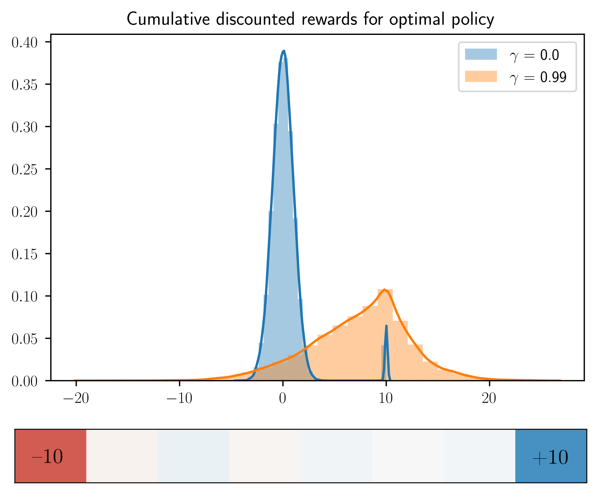
Figure 1: This example illustrates why consideration of the distribution of cumulative discounted future rewards may be more meaningful than of the reward distribution itself: The grid world shown contains a single terminal goal state $s_{\mathrm{goal}}$ with $R(s_{\mathrm{goal}})=+10$, a single terminal fail state $s_{\mathrm{fail}}$ with $R(s_{\mathrm{fail}})=-10$, while for all other states reward values are $R(s)\approx 0$. If the set of non-terminal states ${\mathcal{S}}\smallsetminus\{s_{\mathrm{goal}},s_{\mathrm{fail}}\}$ is large, both optimal policies, which approach $s_{\mathrm{goal}}$ as fast as possible, and highly suboptimal policies, which approach $s_{\mathrm{fail}}$ as fast as possible, spend most time in this region and their reward distributions $P_{R}$ look very much alike: Most of the mass concentrates around 0, and only a small spike at +10 resp. -10 distinguishes them. In contrast, for $\gamma$ tending to 1, the distributions $P_{R}^{(\gamma)}$ for optimal and highly suboptimal policies look increasingly different.

5 Method

The idea on which our method is based is to infer a reward function from demonstrated trajectories together with an estimate of the distribution of (cumulative discounted) rewards that is provided as an input to the algorithm we propose. We refer to this as an optimality profile and denote it by $P_{\mathrm{tgt}}$ (the target we want to match). Our algorithm then tries to find a reward function $R_{\widehat{\theta}}$ within a space of functions ${\mathcal{R}}_{\Theta}=\{R_{\theta}~{}|~{}\theta\in\Theta\}$, such as neural networks of a specific architecture, that minimizes a measure of discrepancy between the optimality profile and the distribution of (discounted) rewards which $R_{\widehat{\theta}}$ induces together with the empirical distribution on ${\mathcal{T}}$:

$$\theta^{*}\in\mathop{\rm arg\,min}_{\theta\in\Theta}\Delta(P_{R_{\theta}}^{(\gamma)},P_{\mathrm{tgt}}),$$ (9)

where $\Delta$ is a metric or divergence measure on the set of probability distributions on $\mathbb{R}$. In our experiments, we use the Wasserstein distance $\Delta=W_{p}$ resp. an entropy-regularized version of it (typically with $p=2$). We will denote the corresponding objective by

$${\mathcal{L}}_{\mathrm{ot}}=W_{p}\big{(}P_{R_{\theta}}^{(\gamma)},P_{\mathrm{tgt}}\big{)},$$ (10)

where “ot” stands for “optimal transport”.

5.1 Symmetry under measure-preserving maps

It may be useful to think of the optimality profile as being induced by a ground truth reward function. The idea is that the requirement of being consistent with the optimality profile induces a strong constraint on the reward function to be found. Ideally, one would hope that a function whose induced distribution is close to the optimality profile should be similar to the ground truth reward function.

However, minima, or approximate minima, of objectives as in (9), which depend on a function only through the push-forward of a given measure, are generally far from unique, due to a large group of symmetries under which such objectives are invariant. In other words, two functions for which these push-forwards are close may still be very different.

Indeed, assume for the moment that we could optimize (9) over the entire space of $\mathbb{R}$-valued functions on ${\mathcal{S}}$, and let $\widehat{R}$ be such a function (we consider the case $\gamma=0$ for simplicity). Let now $\Phi$ be an element of the group of measure-preserving transformations of $({\mathcal{S}},\rho_{\mathcal{S}})$, i.e., a map $\Phi:{\mathcal{S}}\to{\mathcal{S}}$ satisfying $\Phi_{*}\rho_{\mathcal{S}}=\rho_{\mathcal{S}}$. Then we have

$$(\widehat{R}\circ\Phi)_{*}\rho_{\mathcal{S}}=\widehat{R}_{*}(\Phi_{*}\rho_{\mathcal{S}})=\widehat{R}_{*}\rho_{\mathcal{S}},$$ (11)

and hence any objective on functions which only depends on the function through the push-forward of a given measure is invariant under the action of this group. In particular,

$$\Delta(\widehat{R}_{*}\rho_{\mathcal{S}},P_{\mathrm{tgt}})=\Delta((\widehat{R}\circ\Phi)_{*}\rho_{\mathcal{S}},P_{\mathrm{tgt}})$$ (12)

for any $P_{\mathrm{tgt}}$. Since the group of measure-preserving maps is often huge (infinite-dimensional if ${\mathcal{S}}$ is a continuous space), (12) implies that for every local minimum there is a huge subspace of potentially very different functions with the same value of the objective. (Apart from that, our objective is also invariant under the action of the group of measure-preserving maps $(\mathbb{R},P_{\mathrm{tgt}})$, whose elements $\phi$ act by post-composition, i.e., $\widehat{R}\mapsto\phi\circ\widehat{R}$.)

Of course, in reality we do not optimize over the space of all functions ${\mathcal{S}}\to\mathbb{R}$, but only over a subspace ${\mathcal{R}}_{\Theta}$ parametrized by a finite-dimensional parameter $\theta$, which is usually not preserved by the action of the group of measure-preserving maps of $({\mathcal{S}},\rho)$. However, if ${\mathcal{R}}_{\Theta}$ is sufficiently complex, “approximate level sets” of minima will typically still be large. We can therefore not expect our objective (9) to pick a function that is particularly good for our purposes without some additional supervision.

5.2 Additional supervision

In order to deal with the problem described in Section 5.1 in our setting, we propose to use a small amount of additional supervision in order to break the symmetries.

Specifically, we assume that we have access to a small set of pairs of trajectories $\{({\mathbf{s}}_{1},{\mathbf{s}}_{1}^{\prime}),\dots,({\mathbf{s}}_{m},{\mathbf{s}}_{m}^{\prime})\}\subset{\mathcal{T}}\times{\mathcal{T}}$ which are ordered according to ground truth function value, i.e., $R^{(\gamma)}({\mathbf{s}}_{i})\leq R^{(\gamma)}({\mathbf{s}}_{i}^{\prime})$ for all $i$. The corresponding loss component is

$${\mathcal{L}}_{\mathrm{pw}}(R_{\theta})=-\sum_{i=1}^{m}\log\frac{\exp\big{(}R_{\theta}^{(\gamma)}({\mathbf{s}}_{i}^{\prime})\big{)}}{\exp\big{(}R_{\theta}^{(\gamma)}({\mathbf{s}}_{i})\big{)}+\exp\big{(}R_{\theta}^{(\gamma)}({\mathbf{s}}_{i}^{\prime})\big{)}}$$ (13)

which gives a penalty depending on the extent to which the pairs $(R^{(\gamma)}_{\theta}({\mathbf{s}}_{i}),R^{(\gamma)}_{\theta}({\mathbf{s}}_{i}^{\prime}))$ violate the ground truth ordering. This type of loss function, which is related to the classical Bradley–Terry–Luce model of pairwise preferences (Bradley & Terry, 1952; Luce, 1959), has also been used e.g. by (Brown et al., 2019a; Christiano et al., 2017; Ibarz et al., 2018) for learning from preferences in (I)RL settings.

Alternatively, or additionally, we assume that we have access to a small set $\{{\mathbf{s}}_{1},\dots,{\mathbf{s}}_{n}\}\subset{\mathcal{T}}$ of trajectories for which we have ground truth information about returns $y_{i}=R^{(\gamma)}({\mathbf{s}}_{i})$, or noisy versions thereof. Correspondingly, we consider the loss function given by

$${\mathcal{L}}_{\mathrm{fix}}(R_{\theta})=\big{\|}\big{(}R_{\theta}^{(\gamma)}({\mathbf{s}}_{1}),\dots,R_{\theta}^{(\gamma)}({\mathbf{s}}_{n})\big{)}-{\mathbf{y}}\big{\|}_{2},$$ (14)

where ${\mathbf{y}}=(y_{1},\dots,y_{n})$.

To summarize, the objective that we propose to optimize is

$${\mathcal{L}}_{\mathrm{tot}}(R_{\theta})=c_{\mathrm{ot}}{\mathcal{L}}_{\mathrm{ot}}(R_{\theta})+c_{\mathrm{pw}}{\mathcal{L}}_{\mathrm{pw}}(R_{\theta})+c_{\mathrm{fix}}{\mathcal{L}}_{\mathrm{fix}}(R_{\theta}),$$ (15)

a weighted sum of the loss functions discussed above.

6 Algorithm

We assume that we are given a set of demonstrations ${\mathcal{D}}=\{{\mathbf{s}}_{1},\dots,{\mathbf{s}}_{N}\}\subset{\mathcal{T}}$ which are sampled from some policy $\pi$, as well as an optimality profile $P_{\mathrm{tgt}}$ that will serve as the target return distribution for some $\gamma$, and that reflects for example the opinion of a human expert about the degree of optimality of the demonstrations in ${\mathcal{D}}$.

We will also consider the augmented set of trajectories

$$\widetilde{{\mathcal{D}}}=\{{\mathbf{s}}_{1},{\mathbf{s}}_{1}^{[1:]},{\mathbf{s}}_{1}^{[2:]},\dots,{\mathbf{s}}_{N}^{[\ell_{N}-2:]},{\mathbf{s}}_{N}^{[\ell_{N}-1:]}\}$$ (16)

where $\ell_{i}=\ell({\mathbf{s}}_{i})$ and ${\mathbf{s}}^{[j:]}=(s_{j},\dots,s_{\ell({\mathbf{s}})-1})$ is the restriction of ${\mathbf{s}}$ to the time interval $[t,\ell({\mathbf{s}})-1]$. In words, $\widetilde{{\mathcal{D}}}$ consists of all trajectories that one obtains by sampling a trajectory from ${\mathcal{D}}$ and a time step $t\in[0,\ell({\mathbf{s}})-1]$ and then keeping only futures of that time step in ${\mathbf{s}}$; in particular, we have ${\mathcal{D}}\subset\widetilde{{\mathcal{D}}}$. (One could call $\widetilde{{\mathcal{D}}}$ the set of “ends of trajectories in ${\mathcal{D}}$”.) If ${\mathcal{D}}$ is sampled from the trajectory distribution $P_{\mathrm{traj}}$ defined in (1), then $\widetilde{{\mathcal{D}}}\subset{\mathcal{T}}$ is a sample from the distribution $\rho_{{\mathcal{T}}}$ defined in (6).

For notational simplicity, we will recycle notation and denote the elements of $\widetilde{{\mathcal{D}}}$ again by ${\mathbf{s}}_{i}$, that is, $\widetilde{{\mathcal{D}}}=\{{\mathbf{s}}_{1},\dots,{\mathbf{s}}_{M}\}$.

6.1 Stochastic optimization of ${\mathcal{L}}_{\mathrm{ot}}(R_{\theta})$

In every round of Algorithm 2, we need to compute an estimate of the optimal transport loss ${\mathcal{L}}_{\mathrm{ot}}(R_{\theta})$ for the current function $R_{\theta}$ based on a minibatch $B\subset\widetilde{{\mathcal{D}}}$. Algorithm 1 describes how this is done: We first compute the cumulative sum of discounted future rewards $R^{(\gamma)}_{\theta}({\mathbf{s}}_{i})$ for every trajectory ${\mathbf{s}}_{i}\in B$, from which we then compute a histogram $\widehat{P}_{R_{\theta}}^{(\gamma)}(B)$ approximating $P_{R_{\theta}}^{(\gamma)}$, the return distribution for $R_{\theta}$, see (8).

In the next step, we compute an approximately optimal transport plan $G\in\Gamma(\widehat{P}_{R_{\theta}}^{(\gamma)},P_{\mathrm{tgt}})$, i.e., a distribution $G$ on $\mathbb{R}\times\mathbb{R}$ whose marginals are $\widehat{P}_{R_{\theta}}^{(\gamma)}$ and $P_{\mathrm{tgt}}$ and which approximately minimizes the entropy-regularized optimal transport objective

$$\left(\int_{\mathbb{R}\times\mathbb{R}}|x-y|^{p}dG^{\prime}(x,y)\right)^{1/p}-\lambda H(G^{\prime})$$ (17)

among all distributions $G^{\prime}\in\Gamma(\widehat{P}_{R_{\theta}}^{(\gamma)},P_{\mathrm{tgt}})$. Minimizing only the first term in (17) would mean computing an honest optimal transport plan; the entropy term $\lambda H(G^{\prime})$ regularizes the objective, which increases numerical stability. Note that the distributions for which we need to compute a transport plan live in dimension 1, which makes this problem feasible (Cuturi, 2013; Peyré & Cuturi, 2018). In our experiments, we use the Python optimal transport package (Flamary & Courty, 2017) to compute transport plans.

Once we have the transport plan $G$, we sample an element $y_{\mathrm{tgt},j}\sim G(R_{\theta}^{(\gamma)}({\mathbf{s}}_{i_{j}}),\cdot)$ for every trajectory ${\mathbf{s}}_{i_{j}}\in B$; this is a distribution on $\mathbb{R}$ which encodes where the probability mass that $\widehat{P}_{R_{\theta}}^{(\gamma)}$ places on $R_{\theta}^{(\gamma)}({\mathbf{s}}_{i_{j}})\in\mathbb{R}$ should be transported according to the transport plan $G$. Finally, we use the $y_{\mathrm{tgt},j}$ to estimate ${\mathcal{L}}_{\mathrm{ot}}(R_{\theta};B)$.

In spirit, our algorithm has similarity with Wasserstein GANs (Arjovsky et al., 2017), which also attempt to match distributions by minimizing an estimate of the Wasserstein distance (with $p=1$). In contrast to them, we do not make use of Kantorovich-Rubinstein duality to fit a discriminator (which worked much worse for us), but rather work directly with 1d optimal transport plans.

Algorithm 1 Estimation of the optimal transport loss ${\mathcal{L}}_{\mathrm{ot}}$

0:  $B=\{{\mathbf{s}}_{i_{1}},\dots,{\mathbf{s}}_{i_{b}}\}\subset\widetilde{{\mathcal{D}}},P_{\textrm{tgt}}$

1:  Compute $y_{j}=R_{\theta}^{(\gamma)}({\mathbf{s}}_{i_{j}})$ for $j=1,\dots,b$

2:  Use the $y_{i}$ to get an estimate $\widehat{P}_{R_{\theta}}^{(\gamma)}(B)$ of $P_{R_{\theta}}^{(\gamma)}$

3:  Compute a transport plan $G\in\Gamma\big{(}\widehat{P}_{R_{\theta}}^{(\gamma)}(B),P_{\mathrm{tgt}}\big{)}$

4:  Sample $y_{\mathrm{tgt},j}\sim G\big{(}R_{\theta}^{(\gamma)}({\mathbf{s}}_{i_{j}}\big{)},\cdot)$ for $j=1,\dots,b$

5:  ${\mathcal{L}}_{\mathrm{ot}}(R_{\theta};B)=\Big{(}\sum_{j=1}^{b}\big{|}R_{\theta}^{(\gamma)}({\mathbf{s}}_{i_{j}})-y_{\mathrm{tgt},j}\big{|}^{p}\Big{)}^{1/p}$

Algorithm 2 Matching of optimality profiles

0:  ${\mathcal{D}}$, $P_{\mathrm{tgt}}$, ${\mathcal{I}}_{\mathrm{pw}}$, ${\mathcal{Y}}_{\mathrm{fix}}$

1:  Initialize weights $\theta$

2:  for $i=1,\dots,n_{\mathrm{epochs}}$ do

3:     Sample a minibatch $B\subset\widetilde{{\mathcal{D}}}$

4:     Compute ${\mathcal{L}}_{\mathrm{ot}}(R_{\theta};B)$,${\mathcal{L}}_{\mathrm{pw}}(R_{\theta};{\mathcal{I}}_{\mathrm{pw}})$, ${\mathcal{L}}_{\mathrm{fix}}(R_{\theta};{\mathcal{Y}}_{\mathrm{fix}})$

5:     Compute $\nabla_{\theta}{\mathcal{L}}_{\mathrm{tot}}(R_{\theta})$, see (15)

6:     Update weights: $\theta\leftarrow\theta-\eta\nabla_{\theta}{\mathcal{L}}_{\mathrm{tot}}(R_{\theta})$

7:  end for

6.2 Distribution matching with additional supervision

The full distribution matching procedure is summarized by Algorithm 2. In addition to the demonstrations ${\mathcal{D}}$ and the optimality profile $P_{\mathrm{tgt}}$, it takes as its input (a) a set ${\mathcal{Y}}_{\mathrm{fix}}=\{y_{i_{j}},\dots,y_{i_{n}}\in\mathbb{R}\}$ of labels for a subset ${\mathcal{D}}_{\mathrm{fix}}\subset{\mathcal{D}}$, and/or (b) a set ${\mathcal{I}}_{\mathrm{pw}}=\{(j_{1},j_{1}^{\prime}),\dots,(j_{m},j_{m}^{\prime})\in[1,M]^{\times 2}\}$ of ordered pairs of indices of elements of ${\mathcal{D}}$ with respect to which ${\mathcal{L}}_{\mathrm{fix}}(R_{\theta};{\mathcal{Y}}_{\mathrm{fix}})$ (14) resp. ${\mathcal{L}}_{\mathrm{pw}}(R_{\theta};{\mathcal{I}}_{\mathrm{pw}})$ (13) and their gradients are computed in every optimization epoch. The reason we require these additional sourced of supervision is to break symmetries caused by measure-preserving transformations.

In every epoch, we estimate the gradient of the total loss (15) with respect to $\theta$ and then take a step in the direction of the negative gradient. Note that when estimating the gradient $\nabla_{\theta}{\mathcal{L}}_{\mathrm{ot}}(R_{\theta})$ with respect to $\theta$, we treat the target values $y_{\mathrm{tgt},j}$ as constant (line 5 of Algorithm 1), although they really depend on $R_{\theta}$ as well through the optimal transport plan that was computed using an estimate of $P_{R_{\theta}}^{(\gamma)}$.

7 Experiments

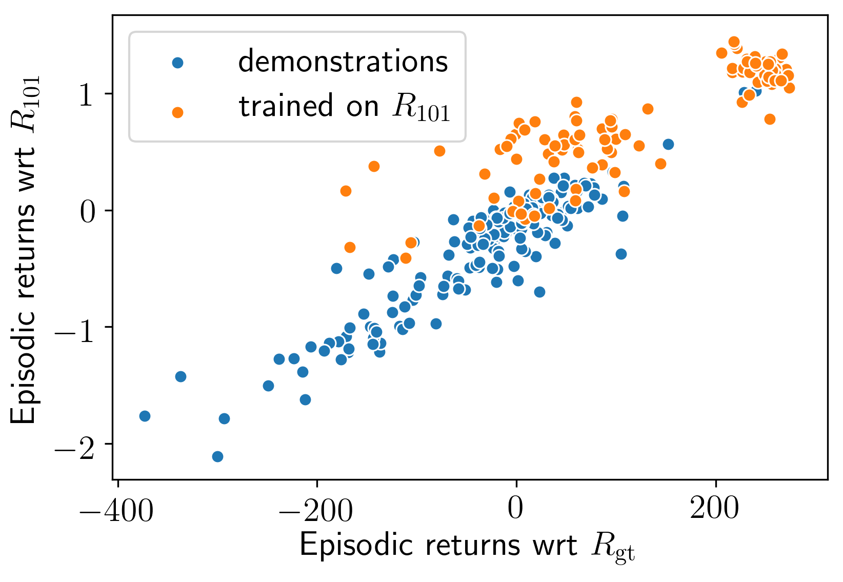
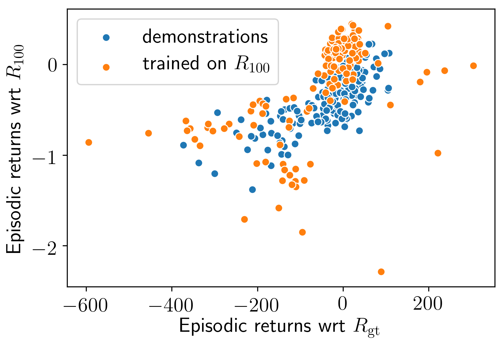
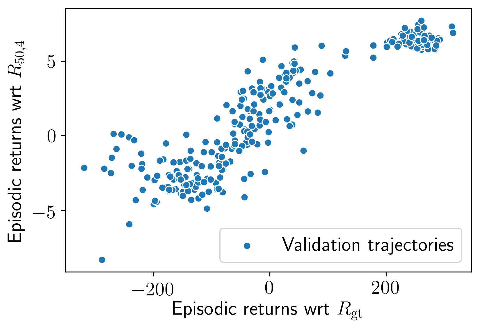
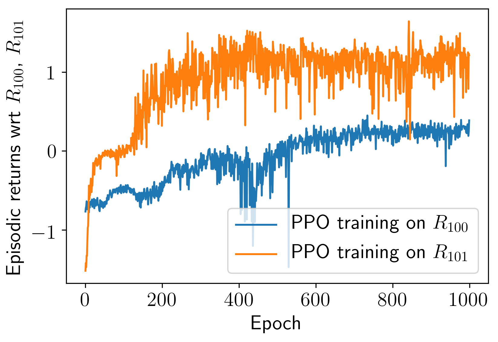
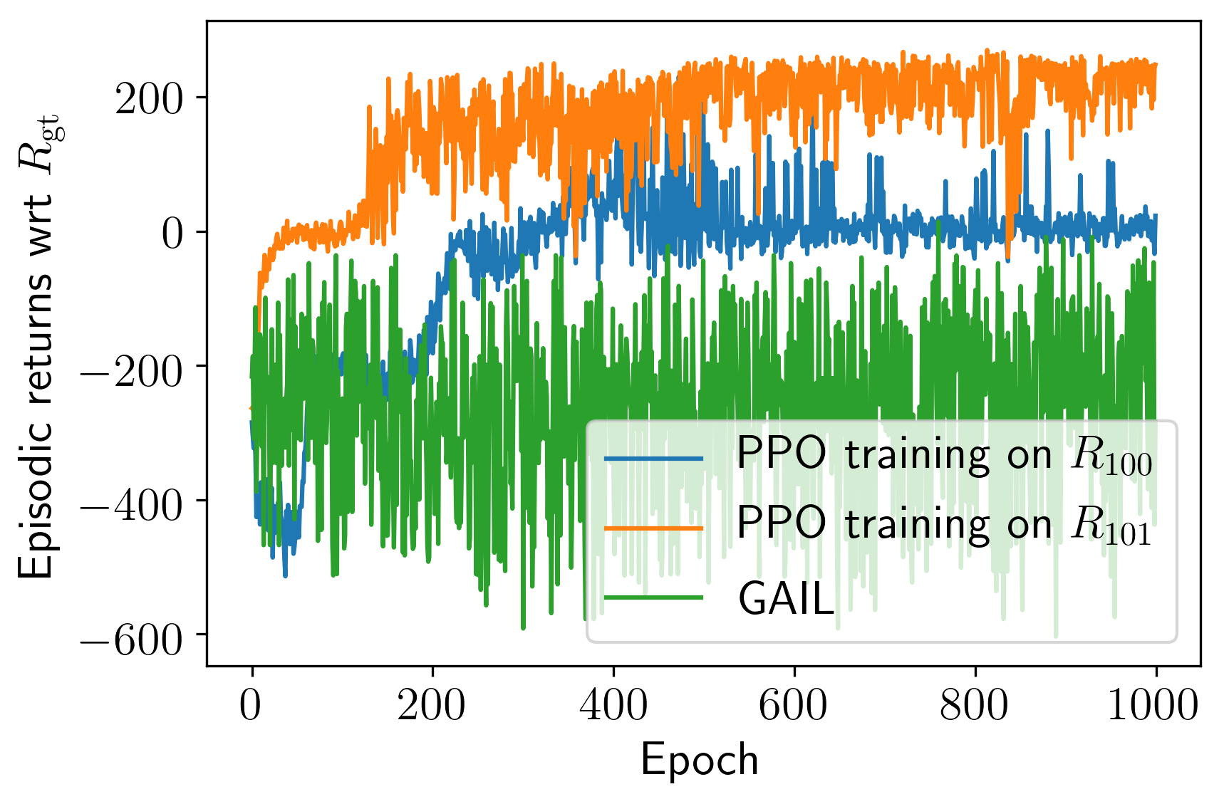
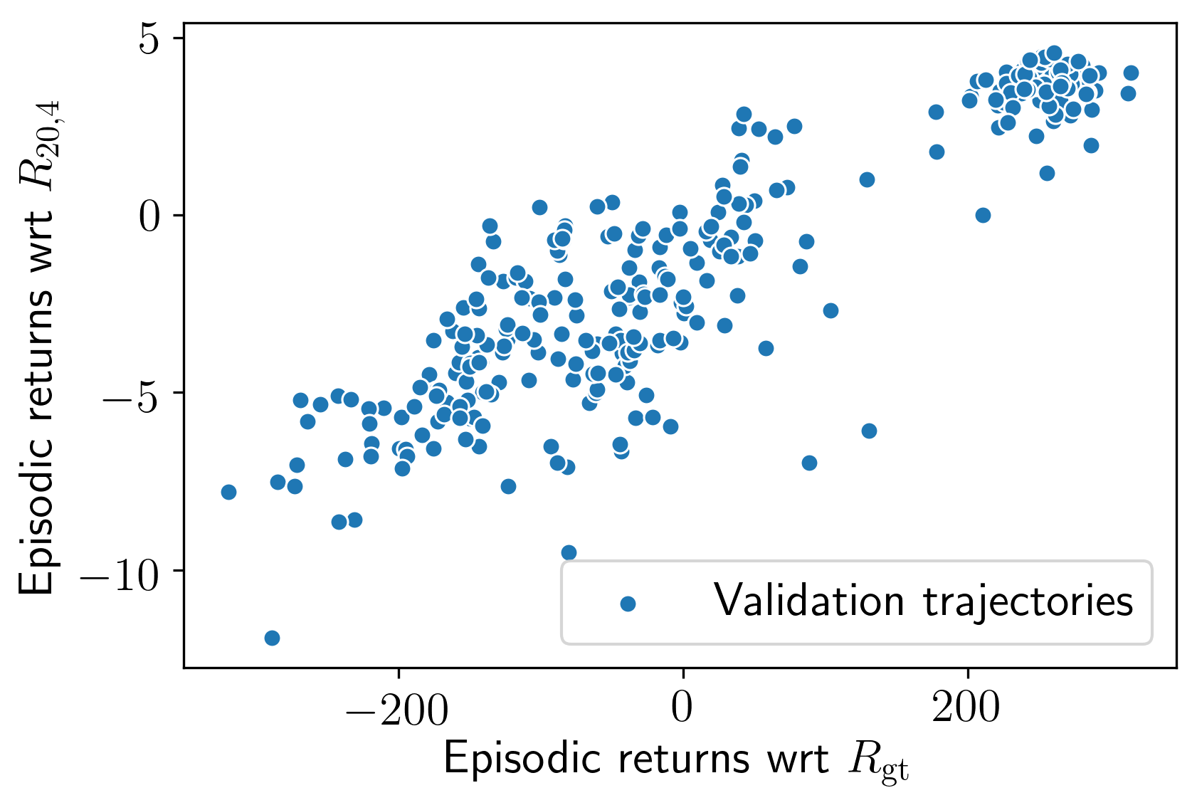
Figure 2: 2 plots ground truth episodic returns versus episodic returns with respect to a learned reward function $R_{101}$; both were evaluated on the demonstrations ${\mathcal{D}}_{101}$ that were used for learning $R_{101}$, and for trajectories generated by policies saved while optimizing a policy for $R_{101}$. 2 shows the same information for a different reward function $R_{100}$ that was trained on different demonstrations ${\mathcal{D}}_{100}$ (see main text). 2 and 2 show the development of episodic return with respect to $R_{100}$ resp. $R_{101}$ and $R_{\mathrm{gt}}$ during PPO training with $R_{100}$ resp. $R_{101}$; Figure 2 also shows the development of episodic returns with respect to $R_{\mathrm{gt}}$ when running GAIL with the demonstrations in ${\mathcal{D}}_{101}$. 2 and 2 show evaluations of two trained reward functions $R_{50,4}$ and $R_{20,4}$ (trained with 50 resp. 20 pairs and 4 fixed points on ${\mathcal{D}}_{125}$) on a large validation set of trajectories. In all plots, the learned reward functions are on a different scale than $R_{\mathrm{gt}}$, as we normalized targets during training and did not invert this afterwards, as we found that PPO was insensitive to scale changes.

We tested our approach in OpenAI Gym’s LunarLander environment, which combines the advantages of being fast to train with algorithms like PPO (Schulman et al., 2017), and having a sufficiently interesting ground truth reward function $R_{\mathrm{gt}}$: The agent receives an immediate small reward or penalty depending on its velocity, distance to the landing region, angle and use of the engines, but there is also a long term component in the form of a bonus of 100 points that the agent can get only once per episode for landing and turning the engines off.

We worked with various sets of demonstrations ${\mathcal{D}}$ created by sampling trajectories from a pool of policies of different qualities. To obtain these, we ran PPO on the ground truth reward function and saved an intermediate policy after every epoch. To obtain the optimality profiles $P_{\mathrm{tgt}}$ required by our algorithm, we computed the ground truth returns for the trajectories in the respective augmented set $\widetilde{\mathcal{D}}$ (16) and produced a histogram (usually with 20 to 50 bins). The trajectories for which we provided ordered index pairs ${\mathcal{I}}_{\mathrm{pw}}$ were sampled randomly, whereas the (few) trajectories for which we provided ground truth labels ${\mathcal{Y}}_{\mathrm{fix}}$ in addition were selected by hand (we took trajectories on which $R_{\mathrm{gt}}^{(\gamma)}$ was close to the minimum or maximum value present in the respective set ${\mathcal{D}}$). We typically used between 10 and 50 pairs and less than 10 fixed points.

The neural network we used to model the reward function was a simple MLP with input dimension 8 (reflecting that $R_{\mathrm{gt}}$ is a function of 8 features), a single hidden layer of dimension 16 and ReLU activations. We optimized the reward function with Adam or RMSprop. For finding a good fit, it usually helped to slowly decrease the learning rate over time, and also to decrease the entropy constant in the regularized optimal transport objective (10). We used a CPU and sometimes an NVIDIA Titan X GPU for training.

7.1 Evaluation of fitted reward functions

We evaluated the quality of our learned reward functions in two different ways: First, we used PPO to train policies optimizing them and then assessed their performance with respect to $R_{\mathrm{gt}}$. The results of that were varied: In some cases, we managed to train policies that were near-optimal at the end of training, meaning that they achieved an average episodic ground truth return $>200$, at which point the environment is viewed as solved, and outperformed (slightly) the performance of the best demonstrations used for fitting the reward function, see Figure 2.

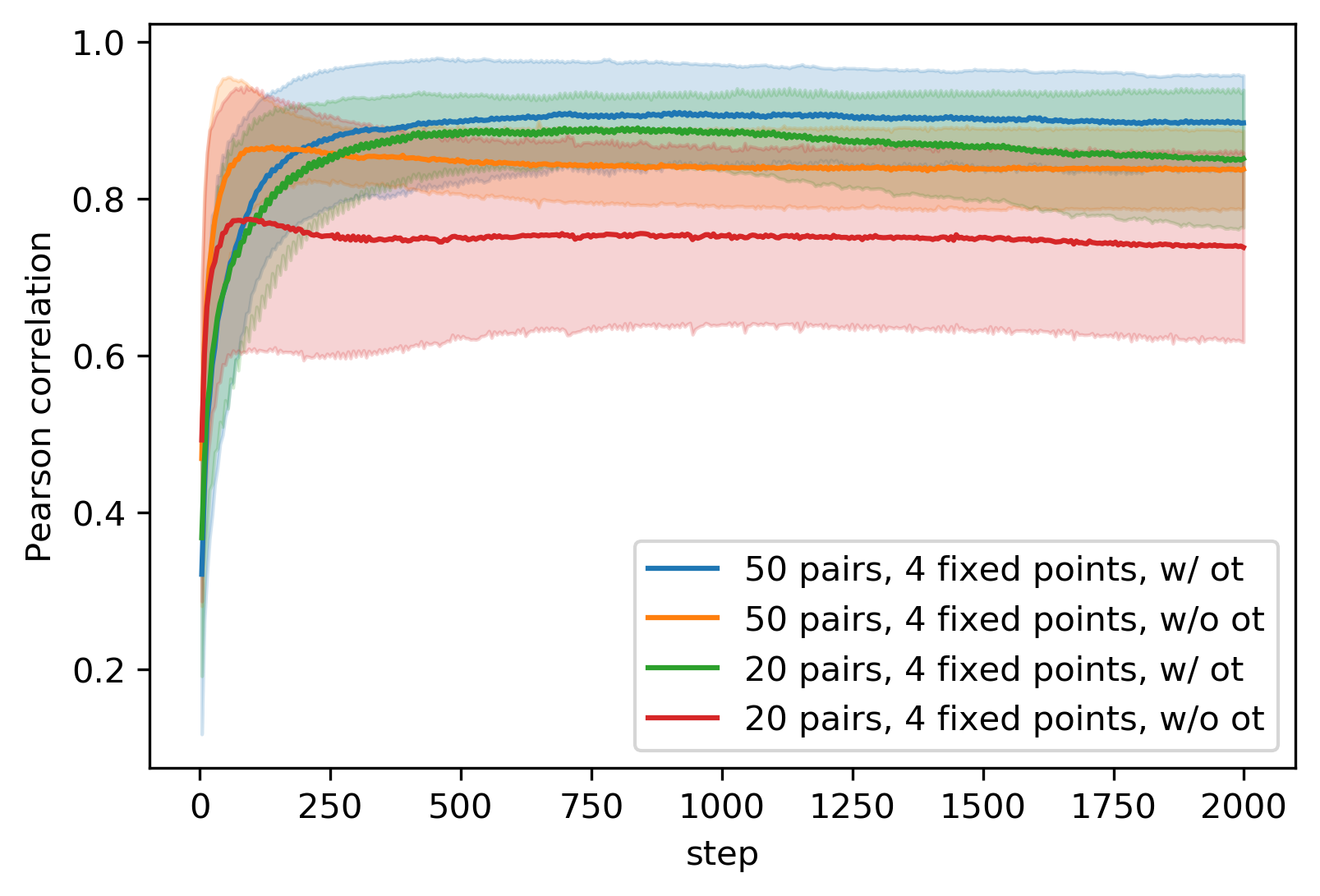
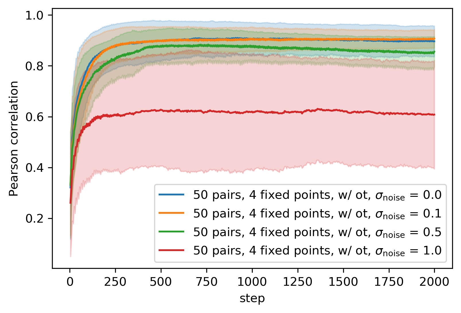
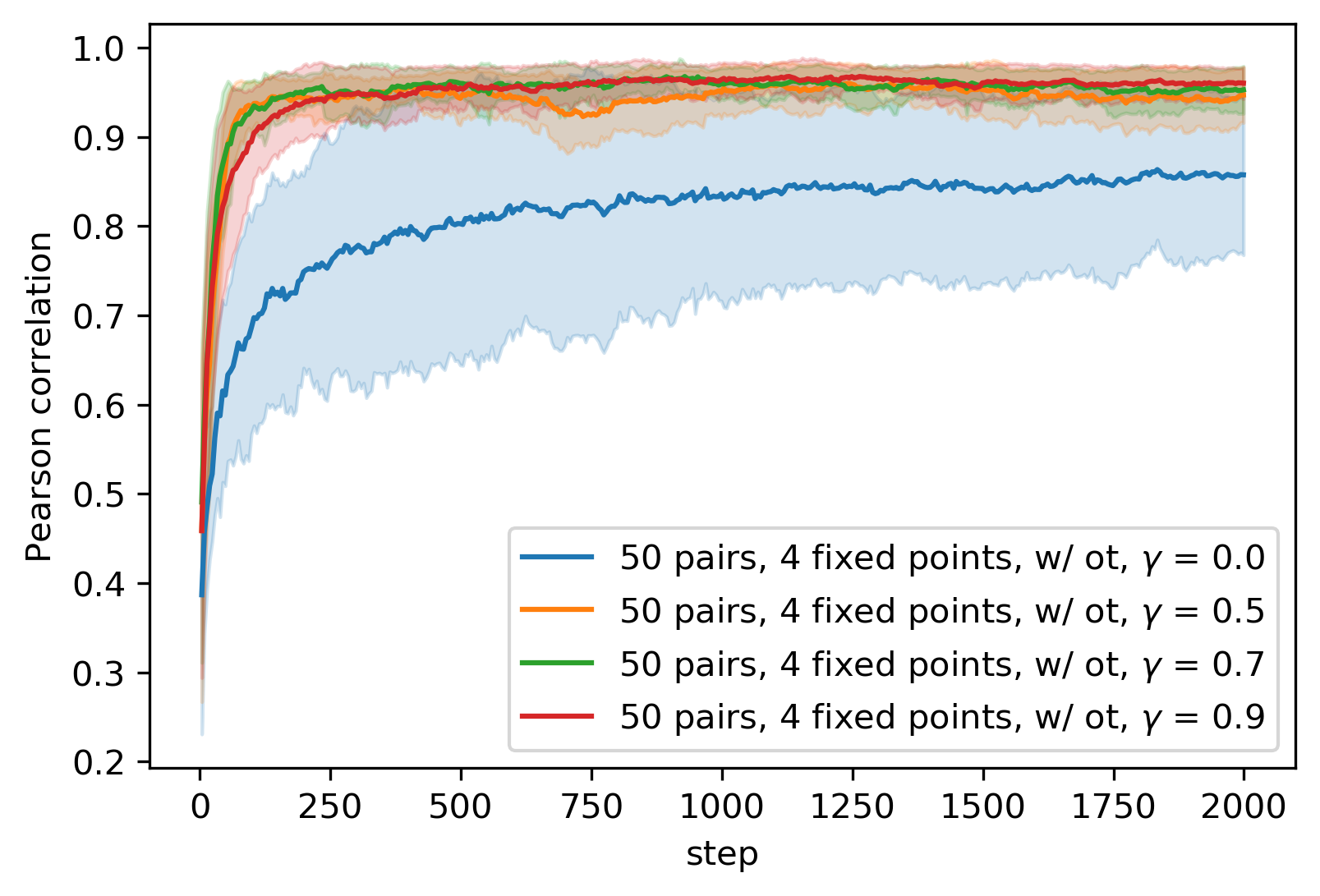
Figure 3: 3 plots the Pearson correlation between then ground truth and the reward learned when our algorithm was given access to 20 resp. 50 pairs in addition to an optimality profile (“w/ ot”), resp. without being given access to an optimality profile (“w/o ot”). In all experiments, 4 points with ground truth information on the discounted reward were provided. 3 plots the Pearson correlation between the ground truth learned reward and the learned reward for various levels of noise applied to the optimality profile provided to our algorithm. 3 plots the Pearson correlation between ground truth and learned reward for various values of the discount factor $\gamma\in\{0,0.5,0.7,0.9\}$ used for computing the optimality profile. All experiments reported in 3, 3, 3 were run with ten different choices of random seed; the plots show means and standard deviations.

Depending on the sets of demonstrations we used, the agent sometimes ended up with policies whose strategy was (i) to drop to the ground without using the engines, (ii) to fly out of the screen, or (iii) approach the landing region and levitate over it. Although suboptimal, these types of policies have ground truth performance much higher than random policies. In general, sets of demonstrations with a high heterogeneity regarding their performance worked better than demonstrations containing e.g. only a few near-optimal trajectories. This is not surprising: If one starts policy training with a random policy, it is clearly important to have an estimate of the reward function which is accurate in regions of the feature space where near-optimal policies do not spend much time.

One set of demonstrations, ${\mathcal{D}}_{100}$ (20000 time steps in total), contained trajectories collected by running 100 policies of low to medium performance. Figure 2 shows an evaluation of the resulting reward function $R_{100}$ both on the trajectories in ${\mathcal{D}}_{100}$ and on trajectories generated by policies saved while optimizing a policy for $R_{100}$. Note that while some of the latter achieved higher ground truth performance than the best demonstration, their performance with respect to $R_{100}$ is mediocre. In the end, the agent learned to levitate over the landing region without actually landing. See videos in the supplementary material.

Another set of demonstrations, ${\mathcal{D}}_{101}$ (21000 time steps in total), was obtained from ${\mathcal{D}}_{100}$ by adding three trajectories generated by a near-optimal policy. Figure 2 shows that the resulting reward function $R_{101}$ was much better correlated with the ground truth reward function than $R_{100}$ and that the policy learned in the end was near-optimal, meaning that the agent managed to land and turn the engines off (and slightly outperformed the best demonstration).

Second, we evaluated our learned reward functions on trajectories sampled from a large set of policies of heterogeneous quality. These policies were produced by running PPO with various hyperparameter configurations to encourage diversity, and saving the intermediate policies after every epoch. Every trajectory in this set corresponded to one full episode that ended as soon as the agent either reached a terminal state (landing and coming to rest, or crash) or completed 1000 time steps. Some results of that for reward functions trained on a large set ${\mathcal{D}}_{125}$ (53000 time steps in total) obtained from ${\mathcal{D}}_{100}$ by adding trajectories sampled from 25 good to optimal policies are shown in Figures 2 and 2.

7.2 Comparison with other methods

Our experiments show that when we do not optimize the optimal transport loss ${\mathcal{L}}_{\mathrm{ot}}$ but only the pairwise loss ${\mathcal{L}}_{\mathrm{pw}}$, the ability of our algorithm to to find a good reward function reduces significantly, unless the number of pairs and fixed points is increased accordingly, see Figure 3. As our method reduces essentially to the TREX method proposed by Brown et al. (2019a) in this case, this indicates that our method can work with significantly fewer pairwise comparisons than TREX provided that an optimality profile is available. We also compared with GAIL (Ho & Ermon, 2016), which was not able to find good policies when provided with the heterogeneous sets of trajectories that we provided to our algorithm, see Figure 2.

7.3 Robustness to noise

We also evaluated the robustness of our method with respect to noise in the optimality profile $P_{\mathrm{tgt}}$ that was provided to our algorithm. To achieve that, we multiplied the cumulative discounted reward values from which the optimality profile was computed with a noise factor sampled from ${\mathcal{N}}(1,\sigma_{\mathrm{noise}})$ for $\sigma_{\mathrm{noise}}\in\{0.1,0.5,1\}$ and provided the resulting histogram to the algorithm. The correlation plot in Figure 3 shows that, while noise clearly affects the ability of the algorithm to match the ground truth closely, small amounts of noise seem to be tolerable.

7.4 Effect of varying the discount factor $\gamma$

We observed that higher values of $\gamma$ tend to lead to better fits of $R_{\mathrm{gt}}$ by the learned reward function, as shown by Figure 3 which plots the development $L_{1}$-distance between the two functions during training for various values of $\gamma$. This may be counter-intuitive, as the supervision that the algorithm gets is computed using $R^{(\gamma)}_{\mathrm{gt}}$, which in some sense approximates $R_{\mathrm{gt}}$ as $\gamma$ gets smaller. However, it seems that the requirement of matching $P_{\mathrm{tgt}}=P_{R_{\mathrm{gt}}}^{(\gamma)}$ actually imposes a stronger constraint on the reward function to be learned as $\gamma$ gets larger.

8 Discussion and outlook

We presented an IRL algorithm that fits a reward function to demonstrations by minimizing the Wasserstein distance to a given optimality profile, that is, a distribution over (cumulative discounted future) rewards which we view as an assessment of the degree of optimality of the demonstrations. To the best of our knowledge, this is the first IRL algorithm that works with this kind of supervision signal. In future work, we will investigate ways of effectively eliciting such optimality profiles from human experts. We also plan to study the objective we propose from an optimization perspective, and to evaluate the performance of our method in high-dimensional settings.

Appendix A Additional explanations regarding state and trajectory distributions

A.1 Distributions on state and trajectory spaces

In the main paper, we claimed that one could interpret the distribution $\rho_{{\mathcal{T}}_{1}}$ on ${\mathcal{T}}\times[0,T]$ resp. ${\mathcal{T}}_{1}=\{({\mathbf{s}},t)\in{\mathcal{T}}\times[0,T]~{}|~{}t\leq\ell({\mathbf{s}})-1\}$ by saying that $\rho_{{\mathcal{T}}_{1}}({\mathbf{s}},t)$ is the probability of obtaining $({\mathbf{s}},t)$ if one first samples a trajectory from ${\mathcal{T}}$ according to a version of $P_{\mathrm{traj}}^{\prime}$ in which probabilities are rescaled proportionally to trajectory length, and then a time step $t$ uniformly at random from $[0,\dots\ell({\mathbf{s}})-1]$. To see that this is indeed the case, note that the rescaled version of $P_{\mathrm{traj}}^{\prime}$ is given by

$$\widetilde{P}_{\mathrm{traj}}^{\prime}({\mathbf{s}})=\frac{\ell({\mathbf{s}})P^{\prime}_{\mathrm{traj}}({\mathbf{s}})}{\sum_{{\mathbf{s}}^{\prime}\in{\mathcal{T}}}\ell({\mathbf{s}}^{\prime})P^{\prime}_{\mathrm{traj}}({\mathbf{s}}^{\prime})}.$$ (18)

Now if we sample ${\mathbf{s}}\sim\widetilde{P}_{\mathrm{traj}}^{\prime}$ and then $t$ uniformly at random from $[0,\dots,\ell({\mathbf{s}})-1]$, the probability of the resulting $({\mathbf{s}},t)$ is

$$\widetilde{P}_{\mathrm{traj}}^{\prime}({\mathbf{s}})\cdot\frac{1}{\ell({\mathbf{s}})}=\frac{P^{\prime}_{\mathrm{traj}}({\mathbf{s}})}{\sum_{{\mathbf{s}}^{\prime}\in{\mathcal{T}}}\ell({\mathbf{s}}^{\prime})P_{\mathrm{traj}}^{\prime}({\mathbf{s}}^{\prime})},$$ (19)

which is the expression for $\rho_{\mathrm{{\mathcal{T}}_{1}}}({\mathbf{s}},t)$ given in equation (3) in the main paper.

To get some intuition for why we consider the rescaled distribution over trajectories, consider the grid world depicted in Figure 4 below and the policy $\pi$ described there. The only two possible trajectories in this setting are a “vertical” trajectory ${\mathbf{s}}_{\mathrm{v}}$ of length 2, and a “horizonal” trajectory ${\mathbf{s}}_{\mathrm{h}}$ of length 8. Note that the non-rescaled trajectory distribution has $P_{\mathrm{traj}}^{\prime}({\mathbf{s}}_{\mathrm{v}})=0.8$ and $P_{\mathrm{traj}}^{\prime}({\mathbf{s}}_{\mathrm{h}})=0.2$, whereas the rescaled trajectory distribution has $\widetilde{P}_{\mathrm{traj}}^{\prime}({\mathbf{s}}_{\mathrm{v}})=0.5$ and $\widetilde{P}_{\mathrm{traj}}^{\prime}({\mathbf{s}}_{\mathrm{h}})=0.5$, reflecting the fact that, in expectation, $\pi$ spends the same amount of time in the vertical as in the horizontal trajectory. We believe that in many situations in which for example human experts are asked to judge behavior it is natural to consider distributions over trajecories that take trajectory length into account, which is why we chose to work with the rescaled trajectory distribution in this paper. However, the method proposed in the paper can also be adapted to other choices.

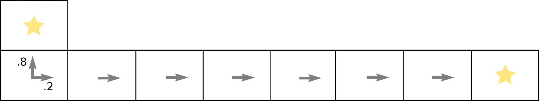
Figure 4: A gridworld to illustrate the difference between the non-rescaled trajectory distribution $P_{\mathrm{traj}}^{\prime}$ and its rescaled version $\widetilde{P}_{\mathrm{traj}}$. We assume an initial state distribution whose mass is concentrated on the state in the lower left corner, so that all trajectories start there. The two states marked with a star are terminal states. The arrows represent a policy $\pi$ which with probability 0.2 moves upwards from the start state and thus ends up in a terminal state immediately, and with probability 0.2 moves to the right from the start state and then continues in that direction until it reaches the terminal state.

A.2 Distributions induced by the reward function

We also claimed that the reward distribution $P_{R}$ could be recovered as the special case of the distribution of cumulative discounted rewards $P_{R}^{(\gamma)}$ for $\gamma=0$, i.e., $P_{R}^{(0)}=P_{R}$. To see that, recall that these distributions are given by

$$P_{R}^{(0)}=R^{(0)}_{*}\rho_{\mathcal{T}}=(R^{(0)})_{*}((\Pi_{\mathcal{T}})_{*}\rho_{{\mathcal{T}}_{1}})=(R^{(0)}\circ\Pi_{\mathcal{T}})_{*}\rho_{{\mathcal{T}}_{1}}$$ (20)

resp.

$$P_{R}=R_{*}\rho_{\mathcal{S}}=R_{*}((\Pi_{\mathcal{S}})_{*}\rho_{{\mathcal{T}}_{1}})=(R\circ\Pi_{\mathcal{S}})_{*}\rho_{{\mathcal{T}}_{1}},$$ (21)

where the maps are those introduced in Section 3. Note that these maps fit in a diagram

(22)

which commutes, meaning that

$$R^{(0)}\circ\Pi_{{\mathcal{T}}}=R\circ\Pi_{{\mathcal{S}}}$$ (23)

Indeed, for $({\mathbf{s}},t)\in{\mathcal{T}}_{1}$, we have

$$R^{(0)}(\Pi_{\mathcal{T}}({\mathbf{s}},t))=R^{(0)}(s_{t},\dots,s_{\ell({\mathbf{s}})-1})=R(s_{t})=R(\Pi_{{\mathcal{S}}}({\mathbf{s}},t)).$$ (24)

(23) together with (20) and (21) implies the claimed equality of distributions $P_{R}^{(0)}=P_{R}$.

References

- Abbeel & Ng (2004) Abbeel, P. and Ng, A. Y. Apprenticeship learning via inverse reinforcement learning. In ICML, 2004.
- Akrour et al. (2011) Akrour, R., Schoenauer, M., and Sebag, M. Preference-based policy learning. In Joint European Conference on Machine Learning and Knowledge Discovery in Databases, pp. 12–27. Springer, 2011.
- Arjovsky et al. (2017) Arjovsky, M., Chintala, S., and Bottou, L. Wasserstein GAN. arXiv:1701.07875 [cs, stat], January 2017. URL http://arxiv.org/abs/1701.07875. arXiv: 1701.07875.
- Bellemare et al. (2017) Bellemare, M. G., Dabney, W., and Munos, R. A distributional perspective on reinforcement learning. In Proceedings of the 34th International Conference on Machine Learning-Volume 70, pp. 449–458. JMLR. org, 2017.
- Bradley & Terry (1952) Bradley, R. A. and Terry, M. E. Rank Analysis of Incomplete Block Designs: I. The Method of Paired Comparisons. Biometrika, 39(3/4):324–345, 1952. ISSN 0006-3444. doi: 10.2307/2334029. URL https://www.jstor.org/stable/2334029.
- Brown et al. (2019a) Brown, D., Goo, W., Nagarajan, P., and Niekum, S. Extrapolating Beyond Suboptimal Demonstrations via Inverse Reinforcement Learning from Observations. In International Conference on Machine Learning, pp. 783–792, May 2019a. URL http://proceedings.mlr.press/v97/brown19a.html.
- Brown et al. (2019b) Brown, D. S., Goo, W., and Niekum, S. Better-than-Demonstrator Imitation Learning via Automatically-Ranked Demonstrations. arXiv:1907.03976 [cs, stat], October 2019b. URL http://arxiv.org/abs/1907.03976. arXiv: 1907.03976.
- Christiano et al. (2017) Christiano, P., Leike, J., Brown, T. B., Martic, M., Legg, S., and Amodei, D. Deep reinforcement learning from human preferences. arXiv:1706.03741 [cs, stat], June 2017. URL http://arxiv.org/abs/1706.03741. arXiv: 1706.03741.
- Cuturi (2013) Cuturi, M. Sinkhorn Distances: Lightspeed Computation of Optimal Transport. In Advances in Neural Information Processing Systems 26, pp. 2292–2300. Curran Associates, Inc., 2013.
- Finn et al. (2016) Finn, C., Levine, S., and Abbeel, P. Guided cost learning: Deep inverse optimal control via policy optimization. In ICML, pp. 49–58, 2016.
- Flamary & Courty (2017) Flamary, R. and Courty, N. Pot python optimal transport library, 2017. URL https://github.com/rflamary/POT.
- Fu et al. (2017) Fu, J., Luo, K., and Levine, S. Learning robust rewards with adversarial inverse reinforcement learning. arXiv preprint arXiv:1710.11248, 2017.
- Ho & Ermon (2016) Ho, J. and Ermon, S. Generative adversarial imitation learning. In NIPS, 2016.
- Ibarz et al. (2018) Ibarz, B., Leike, J., Pohlen, T., Irving, G., Legg, S., and Amodei, D. Reward learning from human preferences and demonstrations in Atari. arXiv:1811.06521 [cs, stat], November 2018. URL http://arxiv.org/abs/1811.06521. arXiv: 1811.06521.
- Levine (2018) Levine, S. Reinforcement Learning and Control as Probabilistic Inference: Tutorial and Review. arXiv:1805.00909 [cs, stat], May 2018. URL http://arxiv.org/abs/1805.00909. arXiv: 1805.00909.
- Luce (1959) Luce, R. D. Individual choice behavior. John Wiley, Oxford, England, 1959.
- Ng & Russell (2000) Ng, A. Y. and Russell, S. J. Algorithms for inverse reinforcement learning. In ICML, 2000.
- Peyré & Cuturi (2018) Peyré, G. and Cuturi, M. Computational Optimal Transport. arXiv:1803.00567 [stat], March 2018. URL http://arxiv.org/abs/1803.00567. arXiv: 1803.00567.
- Schulman et al. (2017) Schulman, J., Wolski, F., Dhariwal, P., Radford, A., and Klimov, O. Proximal Policy Optimization Algorithms. arXiv:1707.06347 [cs], July 2017. URL http://arxiv.org/abs/1707.06347. arXiv: 1707.06347.
- Shiarlis et al. (2016) Shiarlis, K., Messias, J., and Whiteson, S. Inverse Reinforcement Learning from Failure. In Proceedings of the 2016 International Conference on Autonomous Agents & Multiagent Systems, AAMAS ’16, pp. 1060–1068, 2016. ISBN 978-1-4503-4239-1. URL http://dl.acm.org/citation.cfm?id=2936924.2937079.
- Warnell et al. (2018) Warnell, G., Waytowich, N., Lawhern, V., and Stone, P. Deep tamer: Interactive agent shaping in high-dimensional state spaces. In Thirty-Second AAAI Conference on Artificial Intelligence, 2018.
- Wilson et al. (2012) Wilson, A., Fern, A., and Tadepalli, P. A bayesian approach for policy learning from trajectory preference queries. In Advances in neural information processing systems, pp. 1133–1141, 2012.
- Wirth et al. (2017) Wirth, C., Akrour, R., Neumann, G., and Fürnkranz, J. A survey of preference-based reinforcement learning methods. The Journal of Machine Learning Research, 18(1):4945–4990, 2017.
- Wulfmeier et al. (2015) Wulfmeier, M., Ondruska, P., and Posner, I. Maximum entropy deep inverse reinforcement learning. arXiv:1507.04888, 2015.
- Xiao et al. (2019) Xiao, H., Herman, M., Wagner, J., Ziesche, S., Etesami, J., and Linh, T. H. Wasserstein adversarial imitation learning. arXiv preprint arXiv:1906.08113, 2019.
- Ziebart et al. (2008) Ziebart, B. D., Maas, A. L., Bagnell, J. A., and Dey, A. K. Maximum entropy inverse reinforcement learning. In AAAI, 2008.
- Ziebart et al. (2013) Ziebart, B. D., Bagnell, J. A., and Dey, A. K. The principle of maximum causal entropy for estimating interacting processes. IEEE Transactions on Information Theory, 59(4):1966–1980, 2013.