Whale: Efficient Giant Model Training over Heterogeneous GPUs
Abstract
The scaling up of deep neural networks has been demonstrated to be effective in improving model quality, but also encompasses several training challenges in terms of training efficiency, programmability, and resource adaptability. We present Whale, a general and efficient distributed training framework for giant models. To support various parallel strategies and their hybrids, Whale generalizes the programming interface by defining two new primitives in the form of model annotations, allowing for incorporating user hints. The Whale runtime utilizes those annotations and performs graph optimizations to transform a local deep learning DAG graph for distributed multi-GPU execution. Whale further introduces a novel hardware-aware parallel strategy, which improves the performance of model training on heterogeneous GPUs in a balanced manner. Deployed in a production cluster with 512 GPUs, Whale successfully trains an industry-scale multimodal model with over ten trillion model parameters, named M6, demonstrating great scalability and efficiency.
1 Introduction
The training of large-scale deep learning (DL) models has been extensively adopted in various fields, including computer vision[15, 30], natural language understanding[44, 8, 35, 43], machine translation[26, 17], and others. The scale of the model parameters increases from millions to trillions, which significantly improves the model quality [8, 24]; but at the cost of considerable efforts to efficiently distribute the model across GPUs. The commonly used data parallelism () strategy is a poor fit, since it requires the model replicas in GPUs perform gradient synchronization proportional to the model parameter size for every mini-batch, thus easily becoming a bottleneck for giant models. Moreover, training trillions of model parameters requires terabytes of GPU memory at the minimum, which is far beyond the capacity of a single GPU.
To address the aforementioned challenges, a series of new parallel strategies in training DL models have been proposed, including model parallelism (MP) [25], pipeline parallelism [20, 32], etc. For example, differing from the DP approach where each GPU maintains a model replica, MP partitions model parameters into multiple GPUs, avoiding gradient synchronization but instead letting tensors flow across GPUs.
Despite such advancements, new parallel strategies also introduce additional challenges. First, different components of a model might require different parallel strategies. Consider a large-scale image classification task with 100K classes, where the model is composed of [19] for feature extraction and Fully-Connected () layer for classification. The parameter size of is 90 MB, and the parameter size of is 782 MB. If is applied to the whole model, the gradient synchronization of will become the bottleneck. One better solution is to apply to and apply to (Section 2.3). As a result, the synchronization overhead can be reduced by 89.7%, thereby achieving better performance [25].
Additionally, using those advanced parallel strategies increases user efforts significantly. To apply in distributed model training, model developers only need to program the model for one GPU and annotate a few lines, and DL frameworks can replicate the execution plan among multiple GPUs automatically [27]. However, adopting advanced parallelism strategies might make different GPUs process different partitions of the model execution plan, which is difficult to achieve automatically and efficiently [23, 46]. Therefore, significant efforts are required for users to manually place computation operators, coordinate pipeline among mini-batches, implement equivalent distributed operators, and control computation-communication overlapping, etc. [26, 38, 43, 41]. Such an approach exposes low-level system abstractions and requires users to understand system implementation details when programming the models, which greatly increases the amount of user effort.
Further, the training of giant models requires huge computing resources. In industry, the scheduling of hundreds of homogeneous high-end GPUs usually requires a long queuing time. Meanwhile, heterogeneous GPUs can be obtained much easier (e.g., a mixture of P100[2] and V100[3])[21, 47]. But training with heterogeneous GPUs efficiently is even more difficult, since both the computing units and the memory capacity of GPUs need to be considered when building the model. In addition, due to the dynamic scheduling of GPUs, users are unaware of the hardware specification when building their models, which brings a gap between model development and the hardware environment.
We propose Whale, a deep learning framework designed for training giant models. Unlike the aforementioned approaches in which the efficient model partitions are searched automatically or low-level system abstractions and implementation details are exposed to users, we argue that deep learning frameworks should offer high-level abstractions properly to support complicated parallel strategies by utilizing user hints, especially when considering the usage of heterogeneous GPU resources. Guided by this principle, Whale strikes a balance by extending two necessary primitives on top of TensorFlow [7]. Through annotating a local DL model with those primitives, Whale supports all existing parallel strategies and their combinations, which is achieved by automatically rewriting the deep learning execution graph. This design choice decouples the parallel strategies from model code, and lowers them into dataflow graphs, which not only reduces user efforts but also enables graph optimizations and resources-aware optimizations for efficiency and scalability. In this way, Whale eases users from the complicated execution details of giant model training, such as scheduling parallel executions on multiple devices, and balancing computation workload among heterogeneous GPUs. Moreover, Whale introduces a hardware-aware load balancing algorithm when generating a distributed execution plan, which bridges the gap between model development and the heterogeneous runtime environment.
We summarize the key contributions of Whale as follows:
-
1.
For carefully balancing user efforts and distributed graph optimization requirements, Whale introduces two new high-level primitives to express all existing parallel strategies as well as their hybrids.
-
2.
By utilizing the annotations for graph optimization, Whale can transform local models into distributed models, and train them on multiple GPUs efficiently and automatically.
-
3.
Whale proposes a hardware-aware load balancing algorithm, which is seamlessly integrated with parallel strategies to accelerate training on heterogeneous GPUs.
- 4.
Whale has been deployed as a production system for large-scale deep learning training at Alibaba. Using heterogeneous GPUs, further speedup of Bert-Large[13], Resnet50[19], and GNMT[48] from 1.2x to 1.4x can be achieved owing to the hardware-aware load balancing algorithm in Whale. Whale also demonstrates its capabilities in the training of industry-scale models. With only four-line changes to a local model, Whale can train a Multi-Modality to Multi-Modality Multitask Mega-transformer model with 10 billion parameters (M6-10B) on 256 NVIDIA V100 GPUs (32GB), achieving 91% throughput in scalability. What’s more, Whale scales to ten trillion parameters in model training of M6-10T using tensor model parallelism on 512 V100 GPUs (32GB), setting a new milestone in large-scale deep learning model training.
2 Background and Motivation
In this section, we first recap the background of distributed DL model training, especially the parallel strategies for large model training. We then present the importance and the challenges of utilizing heterogeneous GPU resources. Finally, we discuss the gaps and opportunities among existing approaches to motivate the design of a new training framework.
2.1 Parallel Strategies
Deep learning training often consists of millions of iterations, referred to as mini-batches. A typical mini-batch includes several phases to process data for model updating. Firstly, the training data is fed into the model layer-by-layer to calculate a set of scores, known as a forward pass. Secondly, a training loss is calculated between the produced scores and desired scores, which is then utilized to compute gradients for model parameters, referred to as a backward pass. Finally, the gradients scaled by a learning rate are used to update the model parameters and optimizer states.
Data parallelism.
Scaling to multiple GPUs, data parallelism is a commonly adopted strategy where each worker holds a full model replica to process different training data independently. During the backward pass of every mini-batch, the gradients are averaged through worker synchronization. Therefore, the amount of communication is proportional to the model parameter size.
Pipeline Parallelism.
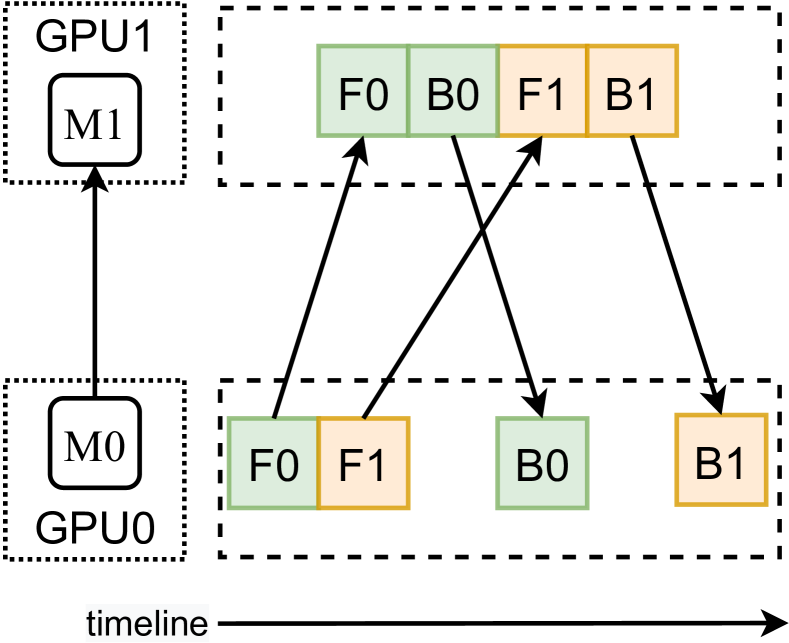
As shown in Figure 4, a DL model is partitioned into two modules, i.e., M0 and M1 (which are also named pipeline stages), which are placed on 2 GPUs respectively. The training data of a mini-batch is split into two smaller micro-batches. In particular, GPU0 starts with the forward of the micro-batch on M0, and then it switches to process the forward of the micro-batch while sending the output of the micro-batch to GPU1. After GPU1 finishes processing forward and backward of the micro-batch on M1, GPU0 continues to calculate the backward pass for M0 after receiving the backward output of M1 from GPU1. Therefore, micro-batches are pipelined among GPUs, which requires the runtime system to balance the load and overlap computation and communication carefully [20, 54, 32, 16]. The model parallelism [12, 11] can be treated as a special case of pipeline parallelism with only one micro-batch.
Tensor Model Parallelism.
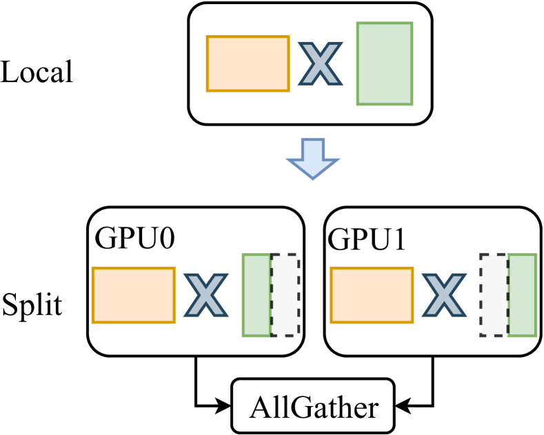
With the growing model size, to process DL operators beyond the memory capacity of the GPU, or to avoid significant communication overhead across model replicas, an operator (or several operators) might be split over multiple GPUs. The tensor model parallelism strategy partitions the input/output tensors and requires an equivalent distributed implementation for the corresponding operator. For example, Figure 4 illustrates the tensor model parallelism strategy for a matmul operator (i.e., matrix multiplication) using 2 GPUs. A matmul operator can be replaced by two matmul operators, wherein each operator is responsible for half of the original computation. An extra all-gather operation is required to merge the distributed results.
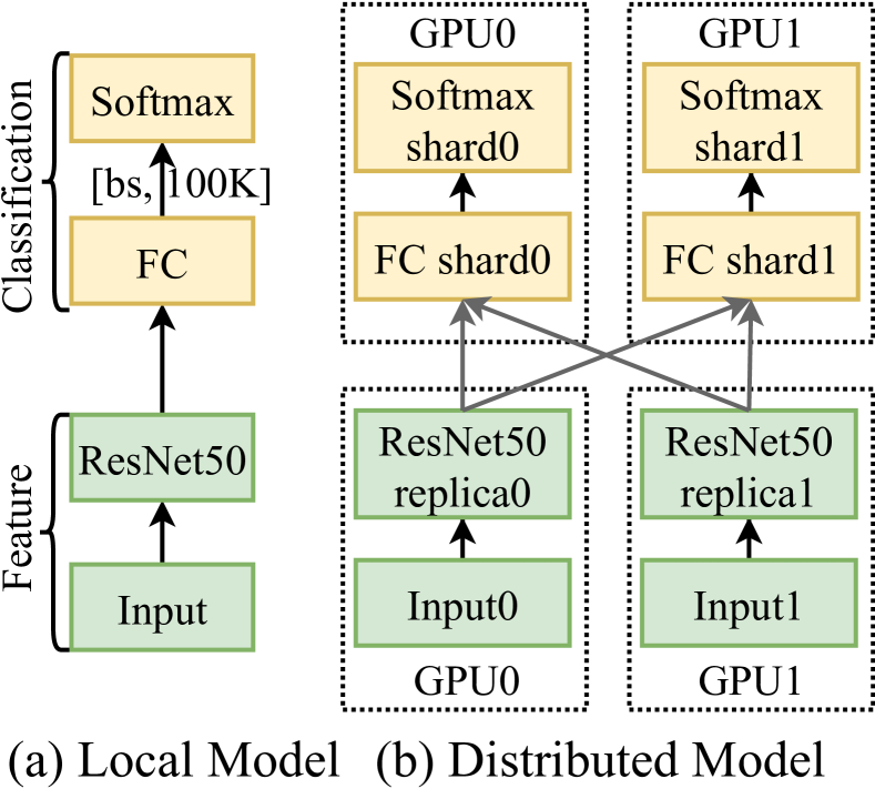
In selecting a proper parallel strategy for model training, both model properties and resources need to be considered. For example, transformer [44] is an important model in natural language understanding, which can be trained efficiently using pipeline parallelism on a few GPUs (e.g., 8 V100 GPUs with NVLINK [4]). However, pipeline parallelism does not scale well with more GPUs (e.g., 64 V100 GPUs). Given more GPUs, each training worker is allocated with fewer operators, of which the GPU computation is not sufficient enough to overlap with the inter-worker communication cost, resulting in poor performance. Therefore, a better solution is to apply hybrid parallelism, where model partitions can be applied with different parallel strategies in combination, and parallel strategies can be nested. Particularly, for the training of a transformer model on 64 GPUs, the model parameters can be partitioned into 8 GPUs using a pipeline strategy, and apply model replica synchronization among 8 pipelined groups using nested data parallelism. Moreover, different parallel strategies can also apply to different model partitions for a hybrid. As an example, a large-scale image classification model (i.e., 100K categories) consists of the image feature extraction partition and the classification partition. The image feature extraction partition requires a significant amount of computation on fewer model parameters. Conversely, the classification partition includes low-computation fully-connected and softmax layers, which are often 10x larger in model size compared to that of image feature extraction. Therefore, adopting a homogeneous parallel strategy will hinder the performance of either partitions. Figure 4 illustrates a better hybrid parallelism approach, in which data parallelism is applied for features extraction partition, tensor model parallelism is adopted for classification partition, and the two are connected.
2.2 Heterogeneity in GPU Clusters
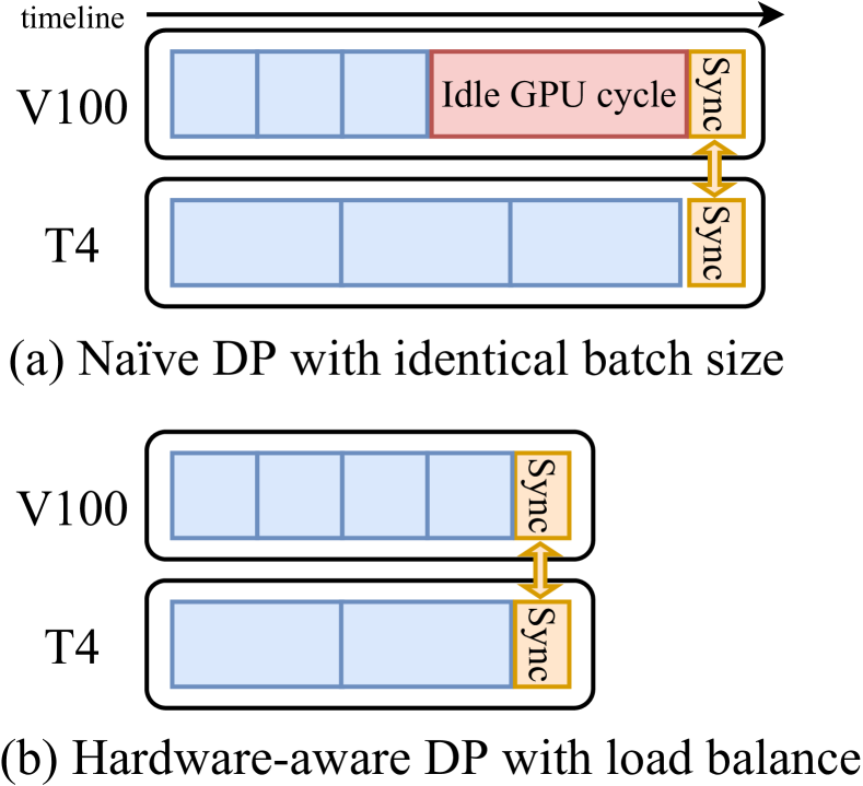
Training a giant model is considerably resource-intensive [33, 17]. Moreover, distributed model training often requires resources to arrive at the same time (i.e., gang schedule [21, 50]). In industry, the shared cluster for giant model training is usually mixed with various types of GPUs (e.g., V100, P100, and T4) for both model training and inference [47]. Training giant models over heterogeneous GPUs lowers the difficulty of collecting all required GPUs (e.g., hundreds or thousands of GPUs) simultaneously, therefore speeding up the model exploration and experiments. However, deep learning frameworks encounter challenges in efficiently utilizing heterogeneous resources. Different types of GPUs are different in terms of GPU memory capacity (e.g., 16GB for P100 and 32GB for V100) and GPU computing capability, which natively introduces an imbalance in computational graph partition and deep learning operator allocation. Figure 4 illustrates training a model using data parallelism on two heterogeneous GPUs, i.e., V100 and T4. The V100 training worker completes forward and backward faster when training samples are allocated evenly, thereby leaving idle GPU cycles before gradient synchronization at the end of every mini-batch. Through the awareness of hardware when dynamically generating an execution plan, Whale allocates more training samples (i.e., batch-size=4) for V100 and the rest of 2 samples for T4 to eliminate the idle waiting time. Combined with advanced parallel strategies and the hybrids over heterogeneous GPUs, different GPU memory capacities and capabilities need to be further considered when partitioning the model for efficient overlapping, which is a complex process (Section 3.3). Model developers can hardly consider all resources issues when programming, and we argue that developers should not have to. A better approach for a general deep learning framework would be automatically generating the execution plan for heterogeneous resources adaptively.
2.3 Gaps and Opportunities
Recent approaches [38, 43, 41, 20, 26] have been proposed for giant model training, however, with limitations as a general DL framework. Firstly, they only support a small number of parallel strategies, which lack a unified abstraction to support all of the parallel strategies and the hybrids thereof. Secondly, significant efforts are required in code modifications to utilize the advanced parallel strategies, compared with local model training and DP approach. Mesh-tensorflow [41] requires the re-implementation of DL operators in a distributed manner. Megatron [43], GPipe [20], DeepSpeed [38], and GShard [26] require user code refactoring using the exposed low-level system primitives or a deep understanding for the implementation of parallel strategies. Thirdly, automatically parallel strategy searching is time-consuming for giant models. Although Tofu [46] and SOAP [23] accomplish model partitioning and replication automatically through computational graph analysis, the search-based graph optimization approach has high computational complexity, which is further positively associated with the number of model operators (e.g., hundreds of thousands of operators for GPT3[8]) and allocated GPUs (e.g., hundreds or thousands), making such an approach impractical when applying to giant model training. Finally, due to the heterogeneity in both GPU computing capability and memory, parallel strategies should be used adaptively and dynamically.
There are significant gaps in supporting giant model training using existing DL frameworks. Exposing low-level interfaces dramatically increases user burden and limits system optimization opportunities. Users need to understand the implementation details of distributed operators and handle the overlapping of computation with communication, which is hard for model developers. Using a low-level approach tightly couples model code to a specific parallel strategy, which requires code rewriting completely when switching between parallel strategies (i.e., from pipeline parallelism to tensor model parallelism). More constraints are introduced to model algorithm innovations, because the efforts of implementing a new module correctly in hybrid strategies are not trivial, let alone consider the performance factors such as load balancing and overlapping. From the system aspect, seeking a better parallel strategy or a combination using existing ones also requires rewriting user code, demanding a deep understanding of the DL model.
To address the aforementioned challenges, Whale explores a new approach that supports various parallel strategies while minimizing user code modifications. By introducing new unified primitives, users can focus on implementing the model algorithm itself, while switching among various parallel strategies by simply changing the annotations. Whale runtime utilizes the user annotations as hints to select parallel strategies at best effort with automatic graph optimization under a limited search scope. Whale further considers heterogeneous hardware capabilities using a balanced algorithm, making resource heterogeneity transparent to users.
3 Design
In this section, we first introduce key abstractions and parallel primitives which can express flexible parallelism strategies with easy programming API (Section 3.1). Then, we describe our parallel planner that transforms a local model with parallel primitives into a distributed model, through partitioning TaskGraphs, inserting bridge layers to connect hybrid strategies, and placing TaskGraphs on distributed devices (Section 3.2). In the end, we propose a hardware-aware load balance algorithm to speed up the training with heterogeneous GPU clusters (Section 3.3).
3.1 Abstraction
3.1.1 Internal Key Concepts
Deep learning frameworks such as TensorFlow[7] provide low-level APIs for distributed computing, but is short of abstractions to represent advanced parallel strategies such as pipeline. The lack of proper abstractions makes it challenging in the understanding and implementation of complicated strategies in a unified way. Additionally, placing model operations to physical devices properly is challenging for complicated hybrid parallel strategies, especially in heterogeneous GPU clusters. Whale introduces two internal key concepts, i.e., TaskGraph and VirtualDevice. TaskGraph is used to modularize operations for applying a parallel strategy. VirtualDevice hides the complexity of mapping operations to physical devices. The two concepts are abstractions of internal system design and are not exposed to users.
TaskGraph(TG) is a subset of the model for parallel transformation and execution. One model can have one or more non-overlapping TaskGraphs. We can apply parallel strategies to each TaskGraph. By modularizing model operations into TaskGraphs, Whale can apply different strategies to different model parts, as well as scheduling the execution of TaskGraphs in a pipeline. A TaskGraph can be further replicated or partitioned. For example, in data parallelism, the whole model is a TaskGraph, which can be replicated to multiple devices. In pipeline parallelism, one pipeline stage is a TaskGraph. In tensor model parallelism, we can shard the TaskGraph into multiple submodules for parallelism.
VirtualDevice (VD) is the logical representation of computing resources, with one VirtualDevice having one or more physical devices. VirtualDevice hides the complexity of device topology, computing capacity as well as device placement from users. One VirtualDevice is assigned to one TaskGraph. Different VirtualDevices are allowed to have different or the same physical devices. For example, VD0 contains physical devices GPU0 and GPU1, VD1 contains physical devices GPU2 and GPU3 (different from VD0), and VD2 contains physical devices GPU0 and GPU1 (the same as VD0).
3.1.2 Parallel Primitives
The parallel primitive is a Python context manager, where operations defined under it are modularized as one TaskGraph. Each parallel primitive has to be configured with a parameter , which is used to generate a VirtualDevice by mapping the number of physical devices. Whale allows users to suggest parallel strategies with two unified primitives, i.e., and . The two primitives can express all existing parallel strategies, as well as a hybrid of them[20, 32, 43, 26, 25].
replicate(device_count) annotates a TaskGraph to be replicated. is the number of devices used to compute the TaskGraph replicas. If is not set, Whale allocates a TaskGraph replica per device. If a TaskGraph is annotated with , it is replicated to devices, with each TaskGraph replica consuming half of the mini-batch. Thus the mini-batch size for one model replica is kept unchanged.
split(device_count) annotates a TaskGraph to apply intra-tensor sharding. The denotes the number of partitions to be sharded. Each sharded partition is placed on one device. For example, shards the TaskGraph into 2 partitions and placed on 2 devices respectively.
The parallel primitives can be used in combination to apply different parallel strategies to different partitions of the model. Additionally, Whale also provides JSON Config API to enable system optimizations. The config is used to enable automatic TaskGraph partitioning given a provided partition number , which further eases the programming for users and is necessary for hardware-aware optimization when resource allocation is dynamic (Section 3.3). In Whale, pipeline parallelism is viewed as an efficient inter-TaskGraph execution strategy. Whale uses the config to enable efficient pipeline parallelism among TaskGraphs when the value is greater than 1. In this way, Whale decouples the generation of TaskGraph from the choice of pipeline parallelism strategies[32, 16, 20]. The system can easily extend to incorporate more pipeline strategies (e.g., swap the execution order of and for M1 in Figure 4).
Besides the combination of parallel strategies or pipeline parallelism, Whale further supports nested data parallelism to the whole parallelized model. Nested data parallelism is enabled automatically when the number of available devices is times of total devices requested by TaskGraphs.
Example 1 shows an example of pipeline parallelism with two TaskGraphs, with each TaskGraph being configured with 1 device. The pipeline parallelism is enabled by configuring the to 8. The total device number of the two TaskGraphs is summed to 2. If the available device number is 8, which is 4 times of total device number, Whale will apply a nested 4-degree data parallelism beyond the pipeline. In contrast, when using two available devices, it is a pure pipeline. Example 2 shows a hybrid strategy that replicates feature part while splitting the model part for the example in Figure 4.
3.2 Parallel Planner
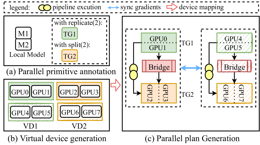
The parallel planner is responsible for producing an efficient parallel execution plan, which is the core of Whale runtime. Figure 5 shows an overview of the parallel planner. The workflow can be described as follows: (a) The parallel planner takes a local model with optional user annotations, computing resources, and optional configs as inputs. The model hyperparameters (e.g., batch size and learning rate), and computing resources (e.g., #GPU and #worker) are decided by the users manually. While the parallel primitive annotations and configs (e.g., and ) could be either be manual or decided by Whale automatically; (b) the VirtualDevices are generated given computing resources and optional annotations automatically (Section 3.2.1); and (c) the model is partitioned into TaskGraphs, and the TaskGraph is further partitioned internally if is annotated. Since we allow applying different strategies to different TaskGraphs, there may exist an input/output mismatch among TaskGraphs. In such case, the planner will insert the corresponding bridge layer automatically between two TaskGraphs (Section 3.2.3).
3.2.1 Virtual Device Generation
VirtualDevices are generated given the number of devices required by each TaskGraph. Given requested physical devices and a model with TaskGraphs, with corresponding device number . For the TaskGraph, Whale will generate a VirtualDevice with number of physical devices. The physical devices are taken sequentially for each VirtualDevice. As mentioned in Section 3.1.2, when the available device number is divisible by the total number of devices requested by all TaskGraphs , Whale will apply a nested DP of -degree to the whole model. In such case, we also replicate the corresponding VirtualDevice for TaskGraph replica. By default, devices are not shared among TaskGraphs. Sharing can be enabled to improve training performance in certain model sharding cases by setting cluster configuration111https://easyparallellibrary.readthedocs.io/en/latest/api/config.html#clusterconfiguration. Whale prefers to place one model replica (with one or more TaskGraphs) within a node, and replicates the model replicas across nodes. Advanced behaviors such as placing TaskGraph replicas within a node to utilize NVLINK for AllReduce communication can be achieved by setting the aforementioned configuration. For example, as shown in Figure 5, there are two TaskGraphs, and each TaskGraph requests 2 GPUs. Two VirtualDevices VD1 and VD2 are generated for two TaskGraphs. VD1 contains and , and VD2 contains and . As the number of available GPUs is 8, which is divisible by the total GPU number of TaskGraphs 4, a replica of VirtualDevices can be generated but with different physical devices.
3.2.2 TaskGraph Partitioning
Whale first partitions a model into TaskGraphs, either by using explicit annotations or automatic system partitioning. If a user annotation is given, operations defined within certain parallel primitive annotation compose a TaskGraph. Otherwise, the system generates TaskGraphs based on the given config parameter and hardware information. The details of the hardware-aware model partitioning is described in Section 3.3.
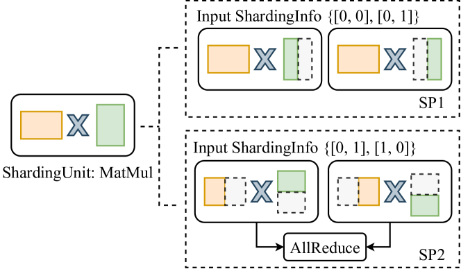
If a TaskGraph is annotated with , Whale will automatically partition it by matching and replacing sharding patterns with a distributed implementation. Before describing the sharding pattern, we introduce two terminologies for tensor model parallelism: 1) ShardingUnit is a basic unit for sharding, and can be an operation or a layer with multiple operations; and 2) ShardingInfo is the tensor sharding information, and is represented as a list given a tensor with dimensions, where represents whether to split the dimension, 1 means true and 0 means false. For example, given a tensor with shape , the ShardingInfo indicates splitting in the second tensor dimension, whereas indicates splitting in both dimensions. A sharding pattern(SP) is a mapping from a ShardingUnit and input ShardingInfo to its distributed implementations. For example, Figure 6 shows two sharding patterns SP1 and SP2 with different input ShardingInfo for ShardingUnit MatMul.
To partition the TaskGraph, Whale first groups the operations in the split TaskGraph into multiple ShardingUnits by hooking TensorFlow ops API222TensorFlow Ops: https://github.com/tensorflow/tensorflow/tree/r1.15/tensorflow/python/ops. The TaskGraph sharding process starts by matching ShardingUnits to the predefined sharding patterns in a topology order. A pattern is matched by a ShardingUnit and input ShardingInfos. If multiple patterns are matched, the pattern with a smaller communication cost is selected. Whale replaces the matched pattern of the original ShardingUnit with its distributed implementation.
3.2.3 Bridge Layer
When applying different parallel strategies to different TaskGraphs, the input/output tensor number and shape may change due to different parallelism degrees or different parallel strategies, thereby resulting in a mismatch of input/output tensor shapes among TaskGraphs. To address the mismatch, Whale proposes a bridge layer to gather the distributed tensors and feed them to the next TaskGraph.
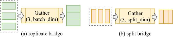
Whale designs two bridge patterns for replicate and split respectively, as shown in Figure 7. For replicate, the TaskGraph is replicated to devices, with different input batches. The bridge layer gathers the outputs from different batches for concatenation in batch dimension . For split, the outputs of TaskGraph are partitioned in split dimension . The bridge layer gathers TaskGraph outputs for concatenation in . By using the bridge layer, each TaskGraph can obtain a complete input tensor. If the gather dimension of the bridge layer is the same as the successor TaskGraph input partition dimension, Whale will optimize by fusing the aforementioned two operations to reduce the communication overhead. As an example, if the outputs of the TaskGraph are gathered in the first dimension, and the inputs of the successor TaskGraph are partitioned in the same dimension, then Whale will remove the above and operations.
3.3 Hardware-aware Load Balance
In this section, we describe how we utilize the hardware information to balance the workloads among TaskGraphs, which achieves high performance even in heterogeneous GPU clusters. The Whale parallel planner obtains the hardware information from the cluster scheduler when the training job is launched, and is responsible for both intra-TaskGraph and inter-TaskGraph load balancing.
3.3.1 Intra-TaskGraph Load Balance
When the allocated devices are homogeneous, by default Whale distributes the workloads within a TaskGraph to multiple devices evenly. However, when allocated with heterogeneous GPUs with different computing capacities (e.g., V100 and P100), the aforementioned identical distribution effectuates suboptimal performance. Such performance can be attributed to a synchronization barrier at the end of TaskGraph execution, which leads to long idle GPU time for the faster GPU, as shown in Figure 4(a). To improve the overall utilization of heterogeneous GPUs, we need to balance the computing according to the device’s computing capacity. The intra-TaskGraph load balance attempts to minimize the idle time within a TaskGraph, which is achieved by balancing the workloads proportional to device computing capacity while being subject to memory constraints. For a TaskGraph annotated with , Whale balances the workload by adjusting the batch size for each TaskGraph replica. The local batch size on heterogeneous devices might differ due to the load balancing strategy (Whale keeps the global batch size unchanged). If batch-sensitive operators such as exist, the local batch differences might have statistical effects. Yet, no users suffer convergence issues when using heterogeneous training in Whale, which is probably due to the robustness of . Besides, techniques like SyncBatchNormaliazaion333https://www.tensorflow.org/api_docs/python/tf/keras/layers/experimental/SyncBatchNormalization might help. For a TaskGraph annotated with , Whale balances the FLOP of a partitioned operation through uneven sharding in splitting dimension among multiple devices.
We profile the TaskGraph on single-precision floating-point operations(FLOP) as and peak memory consumption as . Given GPUs, we collect the information for device including the single-precision FLOP per second as and memory capacity as . Assuming the partitioned load ratio on the device is , we need to find a solution that minimizes the overall GPU waste, which is formulated in Formula 1. We try to minimize the ratio of the computational load of the actual model for each device and the ratio of the computing capacity of the device over the total cluster computing capacity , the maximum workload being bounded by the device memory capacity .
| (1) | ||||
| s.t. |
The load ratio in each device is initialized in proportional to the device’s computing capacity, which ideally results in a most balanced partition. However, when the memory constraint is not satisfied, we need to adjust the load allocation to avoid out-of-memory (OOM) errors, while still trying to achieve good performance. Whale proposes a memory-constraint balancing algorithm to balance the workloads among devices. The main idea of the algorithm is to shift the workload from the memory-overload device to a memory-free device with the lowest computation load. The details of the algorithm are illustrated in Algorithm 1. It takes a TaskGraph and with physical devices as inputs. The algorithm first initializes (line 1-1) the profiling results including 1) as the workload ratios of devices; 2) as the memory utilization of devices; 3) as the FLOP utilization of devices; 4) records out of memory devices whose value in is greater than 1; and 5) records devices that have free memory space. The algorithm then iteratively shifts the load from a memory-overload device to a memory-available device (line 1-1). It first finds a with maximum memory utilization from , then it finds a with available memory space and the lowest FLOP utilization. The function attempts to shift the workload from a to a . For data parallelism, the batch size in the is decreased by , and the batch size in the is increased by . is the maximum number that the will not go after getting the load from the . The profiling information for each device is updated after a successful workload shift is found. The aforementioned process iterates until the are empty or the are empty.
3.3.2 Inter-TaskGraph Load Balance
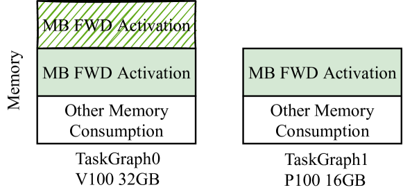
When multiple TaskGraphs are executed in a pipeline, we need to balance the inter-TaskGraph workloads on heterogeneous GPUs. As we introduced in Section 2.1, pipeline parallelism achieves efficient execution by interleaving forward/backward execution among multiple micro-batches. For a model with TaskGraphs, the TaskGraph needs to cache forward activations[32]. Notably, TaskGraph has to cache one more micro-batch forward activation than the previous TaskGraph. Since activation memory is proportional to batch size and often takes a large proportion of the peak memory, e.g., the activation memory VGG16 model with batch size 256 takes up around 74% of the peak memory[18], resulting in uneven memory consumption among different TaskGraphs. The different memory requirements of TaskGraphs motivate us to place earlier TaskGraphs on devices with higher memory capacity. This can be achieved by sorting and reordering the devices in the corresponding VirtualDevice by memory capacity, from higher to lower. Figure 8 shows the memory breakdown of the pipeline example (Figure 4) with two TaskGraphs over heterogeneous GPUs V100 (32GB) and P100 (16GB), we prefer putting TaskGraph0 to V100, which has a higher memory config. The TaskGraph placement heuristic is efficient for common Transformer-based models (i.e., BertLarge and T5 in Figure 18). There might be cases where later stages contain large layers (i.e., large sparse embedding), which can be addressed in Algorithm 1 on handling OOM errors. After reordering the virtual device according to memory requirement, we partition the model operations to TaskGraphs in a topological sort and apply Algorithm 1 to balance the computing FLOP among operations, subject to the memory bound of the memory capacity of each device.
4 Implementation
Whale is implemented as a standalone library without modification of the deep learning framework, which is compatible with TensorFlow1.12 and TensorFlow1.15[7]. The source code of Whale includes 13179 lines of Python code and 1037 lines of C++ code. We have open-sourced444https://github.com/alibaba/EasyParallelLibrary the Whale framework to help giant model training accessible to more users.
Whale enriches the local model with augmented information such as phase information, parallelism annotation, etc., which is crucial to parallelism implementation. To assist the analysis of the user model without modifying the user code, Whale inspects and overwrites TensorFlow build-in functions to capture augmented information. For example, operations are marked as backward when or functions are called.
The parallel strategy is implemented by rewriting the computation graph. We implement a general graph editor module for ease of graph rewriting, which includes functions such as subgraph clone, node replacement, dependency control, and so on. To implement data parallelism, Whale first clones all operations and tensors defined in a local TaskGraph and replaces the device for model replicas. Then it inserts NCCL[6] AllReduce[40] operation to synchronize gradients for each TaskGraph replica. To implement tensor model parallelism, Whale shards the TaskGraph by matching a series of predefined patterns, replacing them with corresponding distributed implementation, and inserting communication operations as needed. To implement pipeline parallelism, Whale builds a pipeline strategy module that supports state-of-the-art strategies[20, 32, 16]. By default, Whale adopts a backward-first strategy which is similar to PipeDream[32]. The pipeline strategy is implemented by first partitioning the minibatch into micro-batches. The interleaving of forward-backward micro-batch execution is achieved by inserting control dependency operations among entrance and exit operations of different TaskGraphs.
To assist hardware-aware optimizations, Whale implements profiling tools that profile the model FLOPS and peak memory consumption. The parallel planner gets the hardware information from our internal GPU cluster, which is used to generate an efficient parallel plan by balancing the computing workloads over heterogeneous GPUs.
5 Experiment
In this section, we first demonstrate the efficiency of the parallelism strategy by evaluating micro-benchmarks. We then evaluate the training with heterogeneous GPUs to show the advantages of the hardware-aware load balance algorithm. We end by showing the effectiveness and efficiency of Whale by two industry-scale multimodal model training cases. All the experiments are conducted on a shared cloud GPU cluster. Every cluster node is equipped with a 96-core Intel Xeon Platinum 8163 (Skylake) @2.50GHz with 736GB RAM, running CentOS 7.7. Each node consists of 2/4/8 GPUs, with NVIDIA 32-GB V100 GPUs[3] or NVIDIA 16-GB P100 GPUs[2], powered by NVIDIA driver 418.87, CUDA 10.0, and cuDNN 7. Nodes are connected by 50Gb/s ethernet. All the models are implemented based on TensorFlow 1.12.
5.1 Micro-benchmark
In this section, we evaluate Whale with a series of micro-benchmarks. We first demonstrate that Whale is efficient in single parallel strategy by comparing with TensorFlow Estimator[14] DP and GPipe[20] pipeline. We then show the advantages of Whale hybrid strategies over single parallel strategy. Next, we measure the overhead of the bridge layer for hybrid strategies. Finally, we evaluate the effect of sharding patterns in automatic TaskGraph partitioning.
5.1.1 Performance of Single Parallel Strategy
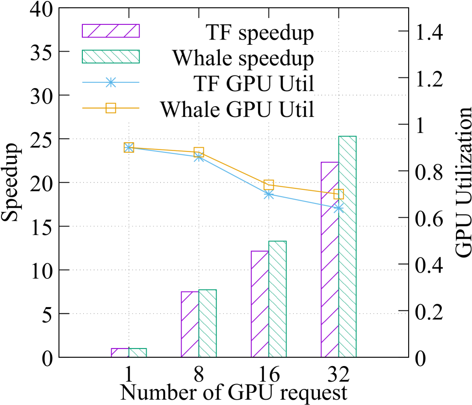
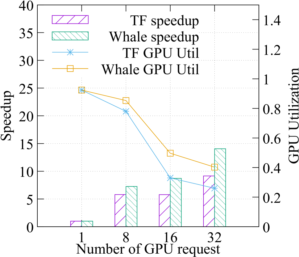
We evaluate Whale DP by comparing it with TensorFlow Estimator DP, using the BertLarge[13] and ResNet50[19] on different number of V100 GPUs. Figure 12 and Figure 12 show the training throughput speedup on ResNet50 and BertLarge respectively. The throughput speedup is calculated by dividing the training throughput on devices by the throughput on one device. Whale DP consistently obtained better speedup and higher GPU utilization than TensorFlow Estimator DP. Such findings could be attributed to Whale’s communication optimization technologies such as hierarchical and grouped AllReduce, which is similar to Horovod[40].
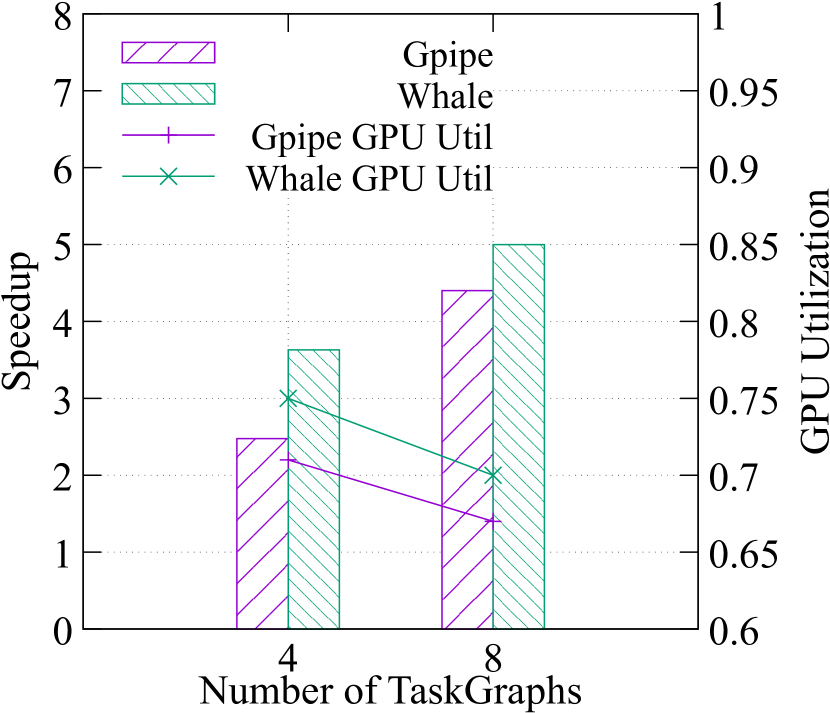
We then evaluate the efficiency of Whale pipeline parallelism by comparing with GPipe[20]. The pipeline scheduling strategy in Whale is similar to PipeDream[32]. The experiments are conducted using the BertLarge model with 4/8 pipeline stages on the different numbers of V100 GPUs. As shown in Figure 12, the training throughput speedup of Whale outperforms GPipe in both 4 stages and 8 stages by 1.45X and 1.14X respectively. We attribute the performance gain to the use of the alternating forward-backward scheduling policy[32], which improves GPU utilization. We also find that the pipeline performance is sensitive to the , thus exposing it as a configurable parameter can help achieve a better performance when models and computing resources change.
5.1.2 Performance of Hybrid Strategy
We evaluate hybrid strategies by comparing them with the single parallel strategy. We also compare the performances of hybrid strategies on different numbers of devices. We select two typical types of hybrid strategies: 1) Nested pipeline with DP; and 2) Combination of DP and tensor model parallelism.
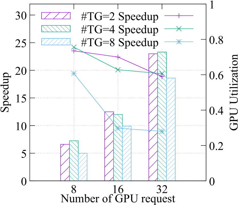
We first apply a nested pipeline with DP to the BertLarge model on V100 GPUs. The model is partitioned into 2/4/8 number of TaskGraphs, and we measure the training performance of each model on 8/16/32 GPUs. Figure 12 shows that pipelines with 2 TaskGraphs and 4 TaskGraphs get similar training speedups and GPU utilization. However, we observe a performance drop on 8 TaskGraphs and lower GPU utilization compared to 2/4 TaskGraphs. This is because 8 TaskGraphs lead to relatively fewer model operations in each TaskGraph, and the GPU computation is not enough to overlap the inter-TaskGraph communication, resulting in poor performance.
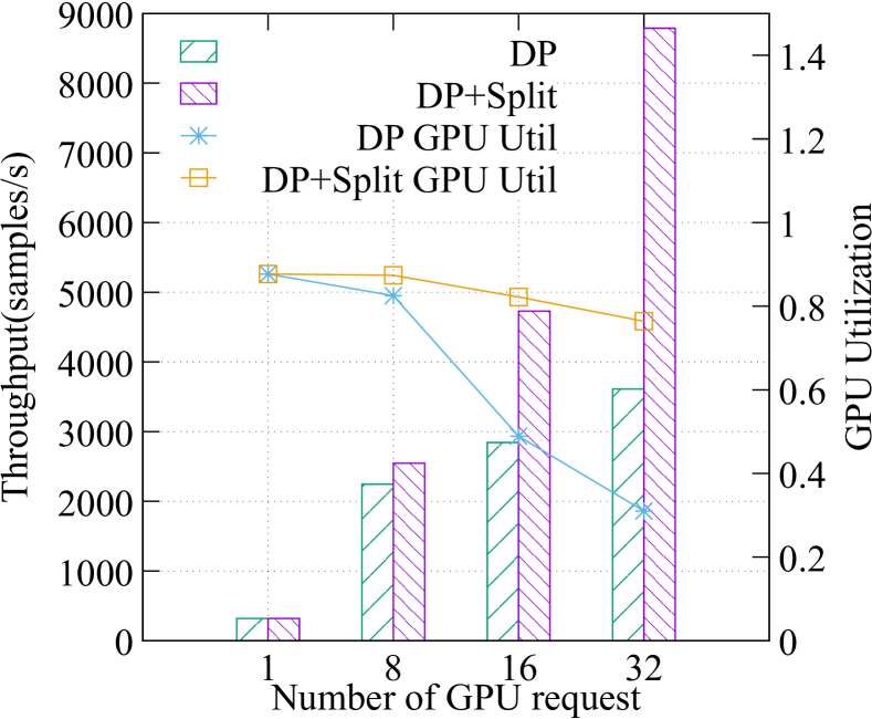
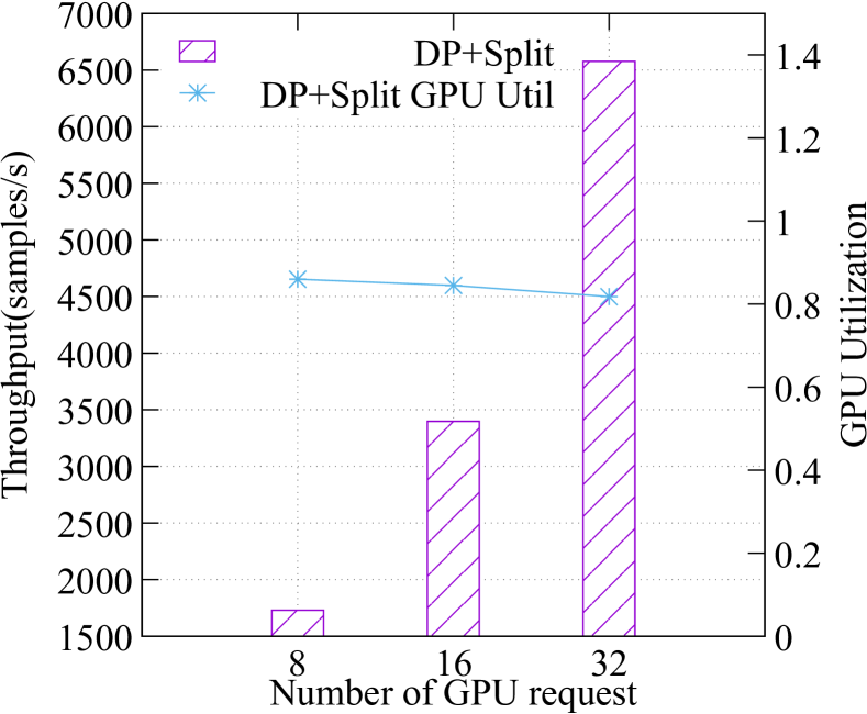
Next, we evaluate the combination hybrid strategy on a large-scale image classification model, as we have discussed in Section 2.1 and illustrated in Figure 4. We perform experiments on classification numbers 100K and 1M on different numbers of V100 GPUs. To reduce the communication overhead of hybrid parallelism, we collocate the replicas with partitions. We compare the hybrid results of 100K classes with DP, as shown in Figure 16, hybrid parallelism outperforms data parallelism by 1.13X, 1.66X, and 2.43X training throughput speedup with 8, 16, and 32 GPUs respectively, with the line plot corresponding to GPU utilization. When the number of workers increases, hybrid parallelism maintains a near-linear speedup, while the DP strategy fails drastically beyond 16 workers. This is because the heavy layer (the parameter size of ResNet50 backbone is 90 MB, while the parameter size of layer is 782MB) incurs a huge gradient synchronization overhead. For the task of 1M classes, DP fails due to OOM. With hybrid parallelism, Whale allows for the training of image classification task with one million classes. Figure 16 shows the performance of hybrid parallelism over 8/16/32 GPUs. The training throughputs from 8 GPUs to 32 GPUs achieve 95% scaling efficiency, which highlights the need for using a hybrid strategy.
5.1.3 Overhead of Bridge Layer
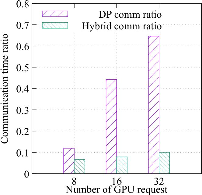
To demonstrate the efficiency of the hybrid strategy, We measure the overhead of the bridge layer by profiling the bridge layer time with 100K classes on 8/16/32 GPUs. We then compare the overhead of gradient AllReduce time in DP with the bridge overhead to understand the performance gain from hybrids. As shown in Figure 16, the overhead of the bridge layer takes around 6% in overall training time in 8 GPUs and 10% in 32 GPUs. The overhead of the hybrid is reduced by 6X on 32 GPUs compared to gradient synchronization overhead of pure DP.
5.1.4 Effect of Sharding Pattern
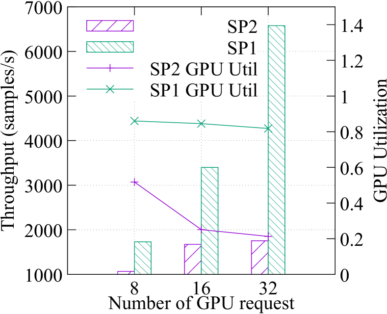
As Whale automatically chooses a sharding pattern with minimum communication cost (Section 3.2.2), to demonstrate the effect of exploring the sharding patterns, we force the framework to use a specific pattern in this experiment. We evaluate two types of sharding patterns as illustrated in Figure 6 on large scale image task with 100K classes. shards the second input tensor in the second tensor dimension, and shards the two input tensors and aggregates the results with . The comparison results of the two sharding patterns are shown in Figure 16, where outperforms by 1.6X to 3.75X as the number of requested GPUs increases from 8 to 32, as has a lower communication cost than . The exploration of sharding patterns allows for the possibility of system optimization in distributed model implementation.
5.2 Performance of Load Balance
We show the benefits of the hardware-aware load balancing algorithm by evaluating data parallelism and pipeline parallelism.
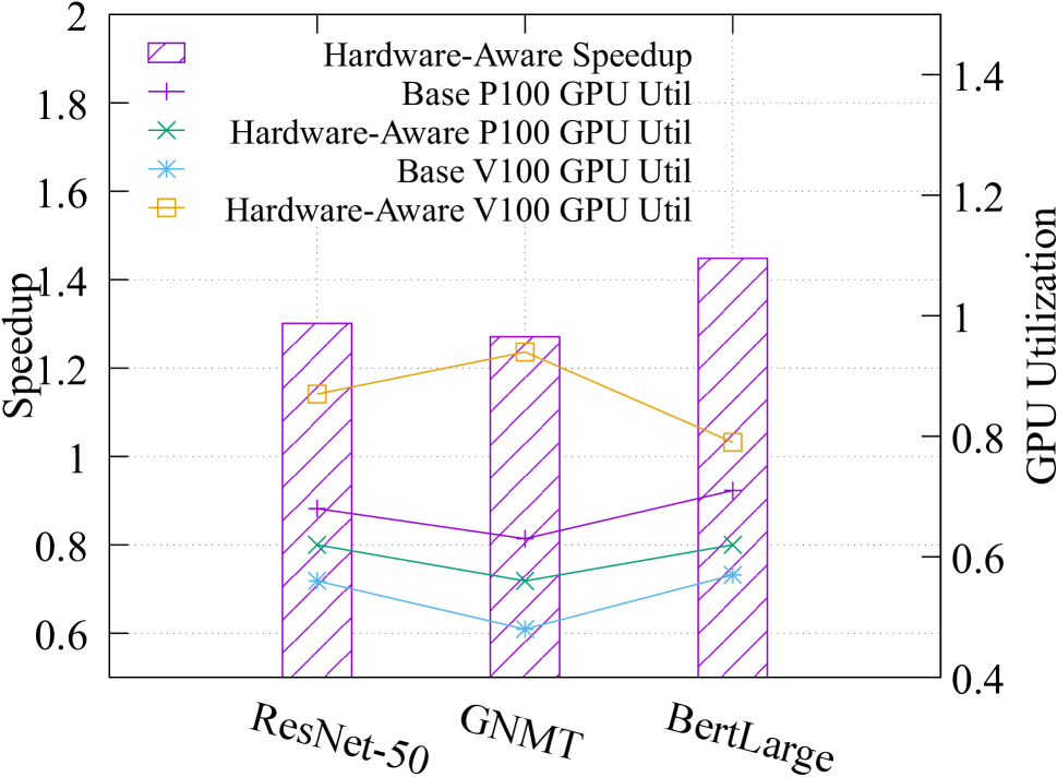
For data parallelism, we evaluate three typical models, including ResNet50, BertLarge, and GNMT[48]. The experiments are conducted on heterogeneous GPUs that consist of 8 32GB V100 GPUs and 8 16GB P100 GPUs. We set the same batch size for all model replicas as the baseline. We then apply the hardware-aware algorithm to each model and get the speedup compared with the baseline performance, as shown in Figure 18. Whale outperforms the baseline in all three models by a factor from 1.3X to 1.4X. We also measure GPU utilization and report the average metric for each GPU type. The hardware-aware policy significantly improves the GPU utilization of V100 by 1.39X to 1.96X for the three models, which improves the overall training performance.
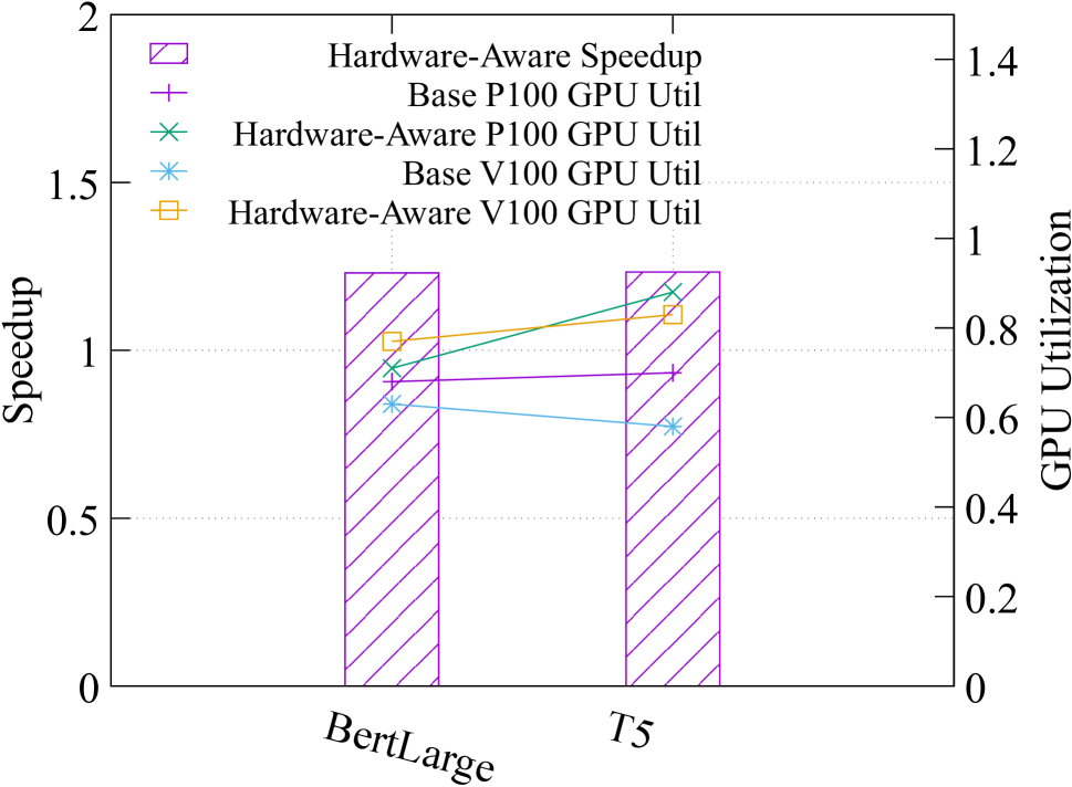
For pipeline parallelism, we evaluate two models, including BertLarge and T5-Large[52]. The training is performed on heterogeneous GPUs that consist of 4 32GB V100 GPUs and 4 16GB P100 GPUs. Both BertLarge and T5-Large are partitioned into 4 stages. We further apply a nested DP to . We set the evenly partitioned model as the baseline. We conducted training with the hardware-aware policy and got about 20% speedup on both models, as shown in Figure 18. The GPU utilization of hardware-aware load balancing strategy improved the GPU utilization of V100 by around 40%, which shows the efficiency of the hardware-aware load balancing algorithm.
5.3 Industry-Scale Giant Model Training
5.3.1 Training M6-10B Model
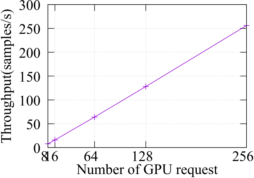
The M6-10B[28] model is a Chinese multimodal model with 10 billion parameters. The model consists of 24 encoder layers and 24 decoder layers. We use Adafactor[42] as the training optimizer. We parallelize the training of M6-10B model with a hybrid parallel strategy, by nesting pipeline parallelism and data parallelism. Whale can easily scale a local M6 model to a distributed one by only adding a few lines on top of the model definition as shown in Example 4. We set the number of pipeline stages to 8 and the number of micro-batches to 35. We enable recomputation[10] to save activation memory during training. The training performance is evaluated on 32-GB V100 GPUs. Each node contains 8 GPUs. When scaling the computing nodes from 8 to 32, Whale achieved 91% scalability, as shown in Figure 19.
5.3.2 Training M6-MoE Model to Trillions
We scale the model parameters to 10 trillion (10T) by switching to hybrids of and tensor model parallelism with only a small number of lines of code change. The computation cost of training dense models is proportional to the model parameters. If we scale the dense 10B model to the dense 10T model linearly without considering overhead, we need at least 256,000 NVIDIA V100 GPUs. Instead of scaling the M6 model with dense structure, we adopt M6-MoE[53] model with sparse expert solution[26, 17]. The sample code of the MoE structure is implemented with Whale by adding four lines, as shown in Example 5. Line 3 sets the default parallel primitive as , i.e., data parallelism is applied for the operations if not explicitly annotated. Line 5 partitions the computation defined under scope across devices.
We evaluate M6-MoE model with 100 billion, 1 trillion and 10 trillion parameters respectively, the detailed configurations can be found in [53, 29]. We enable built-in technologies of Whale to optimize the training process, such as recomputation[10], AMP (auto mixed precision)[1], XLA[5], CPU offloading[39], etc. We can train the M6-MoE-100B model with 100 million samples on 128 V100 in 1.5 days. We advance the model scale to 1 trillion parameters on solely 480 NVIDIA V100 GPUs, in comparison with the recent SOTA on 2048 TPU cores[17]. We further scale the model to 10 trillion parameters by adopting optimized tensor offloading strategies[29] with 512 NVIDIA V100 GPUs. Whale can scale models from 100 billion to 10 trillion without code changes, which makes giant model training accessible to most users.
6 Related Work
Giant model training.
TensorFlow[7] and PyTorch[34] provide well-supported data parallelism and vanilla model parallelism by explicitly assigning operations to specific devices. However, they are not efficient enough for giant model training. Megatron [43], GPipe [20], and Dapple [16] have proposed new parallel training strategies to scale the training of large-scale models. DeepSpeed [38] lacks general support for tensor model parallelism, besides, model layers are required to rewrite in sequential for pipeline parallelism. GShard [26] supports operator splitting by introducing model weight annotations and tensor dimension specifications. The high performance of those works is achieved by exposing low-level system abstractions to users (e.g., device placement, equivalent distributed implementation for operators), or enforcing model or tensor partition manually, which results in significant user efforts. As a parallel work to Whale, GSPMD [51] extends GShard by annotating tensor dimensions mapping for both automatic and manual operator partitioning. As a general giant model training framework, Whale adopts a unified abstraction to express different parallel strategies and their hybrid nests and combinations, utilizing high-level annotations and pattern matching for operator splitting. Whale further scales to M6-10T through automatically distributed graph optimizations with the awareness of heterogeneous resources.
Zero[36, 39, 37] optimizes memory usage by removing redundant GPU memory, offloading computation to the CPU host, and utilizing non-volatile memory respectively. Recomputation[10] trades computation for memory by recomputing tensors from checkpoints. Such memory optimization approaches are orthogonal to Whale, which can be further combined for giant model training efficiently.
Graph optimization.
Deep learning is powered by dataflow graphs with optimizations to rewrite the graph for better performance, such as TensorFlow XLA [7], TVM [9], Ansor [55], AStitish [56], etc. TASO [22] and PET [45] adopt a graph substitution approach to optimize the computation graph automatically. Those works mainly focus on the performance of a single GPU, while Whale utilizes the graph optimization approach for achieving efficient performance in distributed training. Tofu [46] and SOAP [23] also use graph partition to produce distributed execution plans, but with a high search cost. Whale utilizes the introduced annotations to shrink the search space, thus making graph optimization practical for giant model training at a trillion scale. Besides, Whale extends the graph optimization approach to complicated parallel strategies in a unified abstraction, capable of pipeline parallelism, tensor model parallelism, and hybrid parallelism.
Resource heterogeneity.
Philly [21] reports the trace study in multi-tenant GPU clusters of Microsoft and shows the effect of gang scheduling on job queuing. MLaaS [47] studies a two-month trace of a heterogeneous GPU cluster in Alibaba PAI. Gandiva [49] shows jobs are different in sensitivity to allocated resources. Whale is capable of adapting to resource heterogeneity, which can reduce the queuing delay of giant model training with hundreds of GPUs. The design of Whale advocates the approach of decoupling model programming and distributed execution. It dynamically generates an efficient execution plan by considering the properties of both model and heterogeneous resources.
7 Conclusion
Whale demonstrates the possibility of achieving efficiency, programmability, and adaptability in a scalable deep learning framework for training trillion-parameter models. Whale supports various parallel strategies using a unified abstraction, hides distributed execution details through new primitive annotations, and adapts to heterogeneous GPUs with automatic graph optimizations. Going forward, we hope that Whale can become a large-scale deep learning training foundation to further engage model algorithm innovations and system optimizations in parallel, making giant model training technology to be adopted easily and efficiently at scale.
Acknowledgements
We would like to thank our anonymous shepherd and reviewers for their valuable comments and suggestions. We would also like to thank the M6 team and all users of Whale for their help and suggestions.
References
- [1] Automatic mixed precision for deep learning. https://developer.nvidia.com/automatic-mixed-precision.
- [2] Nvidia tesla p100. https://www.nvidia.com/en-us/data-center/tesla-p100/.
- [3] Nvidia v100 tensor core gpu. https://www.nvidia.com/en-us/data-center/v100/.
- [4] NVLink. https://www.nvidia.com/en-us/data-center/nvlink/.
- [5] Xla: Optimizing compiler for machine learning. https://www.tensorflow.org/xla.
- [6] Nccl. https://developer.nvidia.com/nccl, 2019.
- [7] Martín Abadi, Paul Barham, Jianmin Chen, Zhifeng Chen, Andy Davis, Jeffrey Dean, Matthieu Devin, Sanjay Ghemawat, Geoffrey Irving, Michael Isard, et al. Tensorflow: A system for large-scale machine learning. In 12th USENIX symposium on operating systems design and implementation (OSDI 16), pages 265–283, 2016.
- [8] Tom B Brown, Benjamin Mann, Nick Ryder, Melanie Subbiah, Jared Kaplan, Prafulla Dhariwal, Arvind Neelakantan, Pranav Shyam, Girish Sastry, Amanda Askell, et al. Language models are few-shot learners. arXiv preprint arXiv:2005.14165, 2020.
- [9] Tianqi Chen, Thierry Moreau, Ziheng Jiang, Lianmin Zheng, Eddie Yan, Haichen Shen, Meghan Cowan, Leyuan Wang, Yuwei Hu, Luis Ceze, Carlos Guestrin, and Arvind Krishnamurthy. TVM: An automated end-to-end optimizing compiler for deep learning. In 13th USENIX Symposium on Operating Systems Design and Implementation (OSDI 18), pages 578–594, Carlsbad, CA, October 2018. USENIX Association.
- [10] Tianqi Chen, Bing Xu, Chiyuan Zhang, and Carlos Guestrin. Training deep nets with sublinear memory cost. arXiv preprint arXiv:1604.06174, 2016.
- [11] Trishul Chilimbi, Yutaka Suzue, Johnson Apacible, and Karthik Kalyanaraman. Project adam: Building an efficient and scalable deep learning training system. In 11th USENIX Symposium on Operating Systems Design and Implementation (OSDI 14), pages 571–582, Broomfield, CO, October 2014. USENIX Association.
- [12] Jeffrey Dean, Greg S. Corrado, Rajat Monga, Kai Chen, Matthieu Devin, Quoc V. Le, Mark Z. Mao, Marc’Aurelio Ranzato, Andrew Senior, Paul Tucker, Ke Yang, and Andrew Y. Ng. Large scale distributed deep networks. In NIPS, 2012.
- [13] Jacob Devlin, Ming-Wei Chang, Kenton Lee, and Kristina Toutanova. Bert: Pre-training of deep bidirectional transformers for language understanding. arXiv preprint arXiv:1810.04805, 2018.
- [14] Joshua V Dillon, Ian Langmore, Dustin Tran, Eugene Brevdo, Srinivas Vasudevan, Dave Moore, Brian Patton, Alex Alemi, Matt Hoffman, and Rif A Saurous. Tensorflow distributions. arXiv preprint arXiv:1711.10604, 2017.
- [15] Alexey Dosovitskiy, Lucas Beyer, Alexander Kolesnikov, Dirk Weissenborn, Xiaohua Zhai, Thomas Unterthiner, Mostafa Dehghani, Matthias Minderer, Georg Heigold, Sylvain Gelly, et al. An image is worth 16x16 words: Transformers for image recognition at scale. arXiv preprint arXiv:2010.11929, 2020.
- [16] Shiqing Fan, Yi Rong, Chen Meng, Zongyan Cao, Siyu Wang, Zhen Zheng, Chuan Wu, Guoping Long, Jun Yang, Lixue Xia, Lansong Diao, Xiaoyong Liu, and Wei Lin. Dapple: A pipelined data parallel approach for training large models, 2020.
- [17] William Fedus, Barret Zoph, and Noam Shazeer. Switch transformers: Scaling to trillion parameter models with simple and efficient sparsity, 2021.
- [18] Yanjie Gao, Yu Liu, Hongyu Zhang, Zhengxian Li, Yonghao Zhu, Haoxiang Lin, and Mao Yang. Estimating gpu memory consumption of deep learning models. In Proceedings of the 28th ACM Joint Meeting on European Software Engineering Conference and Symposium on the Foundations of Software Engineering, pages 1342–1352, 2020.
- [19] Kaiming He, Xiangyu Zhang, Shaoqing Ren, and Jian Sun. Deep residual learning for image recognition. In Proceedings of the IEEE conference on computer vision and pattern recognition, pages 770–778, 2016.
- [20] Yanping Huang, Youlong Cheng, Ankur Bapna, Orhan Firat, Mia Xu Chen, Dehao Chen, HyoukJoong Lee, Jiquan Ngiam, Quoc V Le, Yonghui Wu, et al. Gpipe: Efficient training of giant neural networks using pipeline parallelism. arXiv preprint arXiv:1811.06965, 2018.
- [21] Myeongjae Jeon, Shivaram Venkataraman, Amar Phanishayee, Junjie Qian, Wencong Xiao, and Fan Yang. Analysis of large-scale multi-tenant GPU clusters for DNN training workloads. In 2019 USENIX Annual Technical Conference (USENIX ATC 19), pages 947–960, 2019.
- [22] Zhihao Jia, Oded Padon, James Thomas, Todd Warszawski, Matei Zaharia, and Alex Aiken. Taso: optimizing deep learning computation with automatic generation of graph substitutions. In Proceedings of the 27th ACM Symposium on Operating Systems Principles, pages 47–62, 2019.
- [23] Zhihao Jia, Matei Zaharia, and Alex Aiken. Beyond data and model parallelism for deep neural networks. In Ameet Talwalkar, Virginia Smith, and Matei Zaharia, editors, Proceedings of Machine Learning and Systems 2019, MLSys 2019, Stanford, CA, USA, March 31 - April 2, 2019. mlsys.org, 2019.
- [24] Jared Kaplan, Sam McCandlish, Tom Henighan, Tom B Brown, Benjamin Chess, Rewon Child, Scott Gray, Alec Radford, Jeffrey Wu, and Dario Amodei. Scaling laws for neural language models. arXiv preprint arXiv:2001.08361, 2020.
- [25] Alex Krizhevsky. One weird trick for parallelizing convolutional neural networks. arXiv preprint arXiv:1404.5997, 2014.
- [26] Dmitry Lepikhin, HyoukJoong Lee, Yuanzhong Xu, Dehao Chen, Orhan Firat, Yanping Huang, Maxim Krikun, Noam Shazeer, and Zhifeng Chen. Gshard: Scaling giant models with conditional computation and automatic sharding. arXiv preprint arXiv:2006.16668, 2020.
- [27] Shen Li, Yanli Zhao, Rohan Varma, Omkar Salpekar, Pieter Noordhuis, Teng Li, Adam Paszke, Jeff Smith, Brian Vaughan, Pritam Damania, and Soumith Chintala. Pytorch distributed: Experiences on accelerating data parallel training. Proc. VLDB Endow., 13(12):3005–3018, 2020.
- [28] Junyang Lin, Rui Men, An Yang, Chang Zhou, Ming Ding, Yichang Zhang, Peng Wang, Ang Wang, Le Jiang, Xianyan Jia, Jie Zhang, Jianwei Zhang, Xu Zou, Zhikang Li, Xiaodong Deng, Jie Liu, Jinbao Xue, Huiling Zhou, Jianxin Ma, Jin Yu, Yong Li, Wei Lin, Jingren Zhou, Jie Tang, and Hongxia Yang. M6: A chinese multimodal pretrainer, 2021.
- [29] Junyang Lin, An Yang, Jinze Bai, Chang Zhou, Le Jiang, Xianyan Jia, Ang Wang, Jie Zhang, Yong Li, Wei Lin, et al. M6-10t: A sharing-delinking paradigm for efficient multi-trillion parameter pretraining. arXiv preprint arXiv:2110.03888, 2021.
- [30] Ze Liu, Yutong Lin, Yue Cao, Han Hu, Yixuan Wei, Zheng Zhang, Stephen Lin, and Baining Guo. Swin transformer: Hierarchical vision transformer using shifted windows. arXiv preprint arXiv:2103.14030, 2021.
- [31] Paulius Micikevicius, Sharan Narang, Jonah Alben, Gregory Diamos, Erich Elsen, David Garcia, Boris Ginsburg, Michael Houston, Oleksii Kuchaiev, Ganesh Venkatesh, et al. Mixed precision training. arXiv preprint arXiv:1710.03740, 2017.
- [32] Deepak Narayanan, Aaron Harlap, Amar Phanishayee, Vivek Seshadri, Nikhil R Devanur, Gregory R Ganger, Phillip B Gibbons, and Matei Zaharia. Pipedream: generalized pipeline parallelism for dnn training. In Proceedings of the 27th ACM Symposium on Operating Systems Principles, pages 1–15, 2019.
- [33] Deepak Narayanan, Mohammad Shoeybi, Jared Casper, Patrick LeGresley, Mostofa Patwary, Vijay Anand Korthikanti, Dmitri Vainbrand, Prethvi Kashinkunti, Julie Bernauer, Bryan Catanzaro, et al. Efficient large-scale language model training on gpu clusters. arXiv preprint arXiv:2104.04473, 2021.
- [34] Adam Paszke, Sam Gross, Francisco Massa, Adam Lerer, James Bradbury, Gregory Chanan, Trevor Killeen, Zeming Lin, Natalia Gimelshein, Luca Antiga, et al. Pytorch: An imperative style, high-performance deep learning library. arXiv preprint arXiv:1912.01703, 2019.
- [35] Colin Raffel, Noam Shazeer, Adam Roberts, Katherine Lee, Sharan Narang, Michael Matena, Yanqi Zhou, Wei Li, and Peter J Liu. Exploring the limits of transfer learning with a unified text-to-text transformer. arXiv preprint arXiv:1910.10683, 2019.
- [36] Samyam Rajbhandari, Jeff Rasley, Olatunji Ruwase, and Yuxiong He. Zero: Memory optimizations toward training trillion parameter models. In SC20: International Conference for High Performance Computing, Networking, Storage and Analysis, pages 1–16. IEEE, 2020.
- [37] Samyam Rajbhandari, Olatunji Ruwase, Jeff Rasley, Shaden Smith, and Yuxiong He. Zero-infinity: Breaking the gpu memory wall for extreme scale deep learning. arXiv preprint arXiv:2104.07857, 2021.
- [38] Jeff Rasley, Samyam Rajbhandari, Olatunji Ruwase, and Yuxiong He. Deepspeed: System optimizations enable training deep learning models with over 100 billion parameters. In Proceedings of the 26th ACM SIGKDD International Conference on Knowledge Discovery & Data Mining, pages 3505–3506, 2020.
- [39] Jie Ren, Samyam Rajbhandari, Reza Yazdani Aminabadi, Olatunji Ruwase, Shuangyan Yang, Minjia Zhang, Dong Li, and Yuxiong He. Zero-offload: Democratizing billion-scale model training. arXiv preprint arXiv:2101.06840, 2021.
- [40] Alexander Sergeev and Mike Del Balso. Horovod: fast and easy distributed deep learning in tensorflow. arXiv preprint arXiv:1802.05799, 2018.
- [41] Noam Shazeer, Youlong Cheng, Niki Parmar, Dustin Tran, Ashish Vaswani, Penporn Koanantakool, Peter Hawkins, HyoukJoong Lee, Mingsheng Hong, Cliff Young, et al. Mesh-tensorflow: Deep learning for supercomputers. In Advances in Neural Information Processing Systems, pages 10414–10423, 2018.
- [42] Noam Shazeer and Mitchell Stern. Adafactor: Adaptive learning rates with sublinear memory cost. In International Conference on Machine Learning, pages 4596–4604. PMLR, 2018.
- [43] Mohammad Shoeybi, Mostofa Patwary, Raul Puri, Patrick LeGresley, Jared Casper, and Bryan Catanzaro. Megatron-lm: Training multi-billion parameter language models using model parallelism. arXiv preprint arXiv:1909.08053, 2019.
- [44] Ashish Vaswani, Noam Shazeer, Niki Parmar, Jakob Uszkoreit, Llion Jones, Aidan N Gomez, Lukasz Kaiser, and Illia Polosukhin. Attention is all you need. arXiv preprint arXiv:1706.03762, 2017.
- [45] Haojie Wang, Jidong Zhai, Mingyu Gao, Zixuan Ma, Shizhi Tang, Liyan Zheng, Yuanzhi Li, Kaiyuan Rong, Yuanyong Chen, and Zhihao Jia. PET: Optimizing tensor programs with partially equivalent transformations and automated corrections. In 15th USENIX Symposium on Operating Systems Design and Implementation (OSDI 21), pages 37–54, 2021.
- [46] Minjie Wang, Chien-Chin Huang, and Jinyang Li. Supporting very large models using automatic dataflow graph partitioning. In George Candea, Robbert van Renesse, and Christof Fetzer, editors, Proceedings of the Fourteenth EuroSys Conference 2019, Dresden, Germany, March 25-28, 2019, pages 26:1–26:17. ACM, 2019.
- [47] Qizhen Weng, Wencong Xiao, Yinghao Yu, Wei Wang, Cheng Wang, Jian He, Yong Li, Liping Zhang, Wei Lin, and Yu Ding. MLaaS in the wild: Workload analysis and scheduling in large-scale heterogeneous gpu clusters. In 19th USENIX Symposium on Networked Systems Design and Implementation (NSDI 22). USENIX Association, 2022.
- [48] Yonghui Wu, Mike Schuster, Zhifeng Chen, Quoc V Le, Mohammad Norouzi, Wolfgang Macherey, Maxim Krikun, Yuan Cao, Qin Gao, Klaus Macherey, et al. Google’s neural machine translation system: Bridging the gap between human and machine translation. arXiv preprint arXiv:1609.08144, 2016.
- [49] Wencong Xiao, Romil Bhardwaj, Ramachandran Ramjee, Muthian Sivathanu, Nipun Kwatra, Zhenhua Han, Pratyush Patel, Xuan Peng, Hanyu Zhao, Quanlu Zhang, Fan Yang, and Lidong Zhou. Gandiva: Introspective cluster scheduling for deep learning. In 13th USENIX Symposium on Operating Systems Design and Implementation, OSDI 2018, Carlsbad, CA, USA, October 8-10, 2018, pages 595–610. USENIX Association, 2018.
- [50] Wencong Xiao, Shiru Ren, Yong Li, Yang Zhang, Pengyang Hou, Zhi Li, Yihui Feng, Wei Lin, and Yangqing Jia. Antman: Dynamic scaling on GPU clusters for deep learning. In 14th USENIX Symposium on Operating Systems Design and Implementation (OSDI 20), pages 533–548. USENIX Association, November 2020.
- [51] Yuanzhong Xu, HyoukJoong Lee, Dehao Chen, Blake Hechtman, Yanping Huang, Rahul Joshi, Maxim Krikun, Dmitry Lepikhin, Andy Ly, Marcello Maggioni, et al. Gspmd: General and scalable parallelization for ml computation graphs. arXiv preprint arXiv:2105.04663, 2021.
- [52] Linting Xue, Noah Constant, Adam Roberts, Mihir Kale, Rami Al-Rfou, Aditya Siddhant, Aditya Barua, and Colin Raffel. mt5: A massively multilingual pre-trained text-to-text transformer. arXiv preprint arXiv:2010.11934, 2020.
- [53] An Yang, Junyang Lin, Rui Men, Chang Zhou, Le Jiang, Xianyan Jia, Ang Wang, Jie Zhang, Jiamang Wang, Yong Li, et al. Exploring sparse expert models and beyond. arXiv preprint arXiv:2105.15082, 2021.
- [54] Bowen Yang, Jian Zhang, Jonathan Li, Christopher Ré, Christopher Aberger, and Christopher De Sa. Pipemare: Asynchronous pipeline parallel dnn training. Proceedings of Machine Learning and Systems, 3, 2021.
- [55] Lianmin Zheng, Chengfan Jia, Minmin Sun, Zhao Wu, Cody Hao Yu, Ameer Haj-Ali, Yida Wang, Jun Yang, Danyang Zhuo, Koushik Sen, et al. Ansor: Generating high-performance tensor programs for deep learning. In 14th USENIX Symposium on Operating Systems Design and Implementation (OSDI 20), pages 863–879, 2020.
- [56] Zhen Zheng, Xuanda Yang, Pengzhan Zhao, Guoping Long, Kai Zhu, Feiwen Zhu, Wenyi Zhao, Xiaoyong Liu, Jun Yang, Jidong Zhai, Shuaiwen Leon Song, and Wei Lin. Astitch: Enabling a new multi-dimensional optimization space for memory-intensive ml training and inference on modern simt architectures. In Proceedings of the 27th ACM International Conferenceon Architectural Support for Programming Languages and Operating Systems. ACM, 2022.