How important are the residual nonadiabatic couplings for an accurate simulation of nonadiabatic quantum dynamics in a quasidiabatic representation?

Abstract

Diabatization of the molecular Hamiltonian is a standard approach to removing the singularities of nonadiabatic couplings at conical intersections of adiabatic potential energy surfaces. In general, it is impossible to eliminate the nonadiabatic couplings entirely—the resulting “quasidiabatic” states are still coupled by smaller but nonvanishing residual nonadiabatic couplings, which are typically neglected. Here, we propose a general method for assessing the validity of this potentially drastic approximation by comparing quantum dynamics simulated either with or without the residual couplings. To make the numerical errors negligible to the errors due to neglecting the residual couplings, we use the highly accurate and general eighth-order composition of the implicit midpoint method. The usefulness of the proposed method is demonstrated on nonadiabatic simulations in the cubic Jahn–Teller model of nitrogen trioxide and in the induced Renner–Teller model of hydrogen cyanide. We find that, depending on the system, initial state, and employed quasidiabatization scheme, neglecting the residual couplings can result in wrong dynamics. In contrast, simulations with the exact quasidiabatic Hamiltonian, which contains the residual couplings, always yield accurate results.

I Introduction

The celebrated Born–Oppenheimer approximation,[1] which treats the electronic and nuclear motions in molecules separately, is no longer valid for describing processes involving two or more strongly vibronically coupled electronic states. A common approach that goes beyond this approximation[2, 3, 4, 5, 6, 7, 8, 9] consists in solving the time-dependent Schrödinger equation with a truncated molecular Hamiltonian that includes only a few, most significantly coupled[10, 11] Born–Oppenheimer electronic states.[12, 13, 14] The “adiabatic” states, obtained directly from the electronic structure calculations, are, however, not adequate for representing the molecular Hamiltonian in the region of strong nonadiabatic couplings; in particular, the couplings between the states diverge at conical intersections,[15, 16, 17, 18, 2, 14, 19] where potential energy surfaces of two or more adiabatic states intersect.

Quasidiabatization, i.e., a coordinate-dependent unitary transformation[20, 21, 22] of the molecular Hamiltonian that reduces the magnitude of the nonadiabatic vector couplings, rectifies this singularity. The transformation matrix can be obtained by various quasidiabatization schemes, of which a few representative examples include methods based on the integration of the nonadiabatic couplings[23, 24, 25, 26, 27, 28, 29, 30, 31, 32, 33] or on different molecular properties[34, 35, 36, 37, 38, 39, 40] and the block-diagonalization[41, 42, 43, 44] or regularized diabatization[45, 46, 47] schemes.

In systems with more than one nuclear degree of freedom, the strict diabatization, which eliminates the nonadiabatic couplings completely, is only possible if infinitely many electronic states are considered.[48, 21] The best one can do for a general subsystem with a finite number of electronic states is the above-mentioned quasidiabatization, in which the unitary transformation reduces the magnitude of the couplings but does not remove them entirely. However, it is a common practice to neglect these nonvanishing “residual” couplings present in the exact quasidiabatic Hamiltonian and thus obtain an approximate quasidiabatic Hamiltonian, whose additional benefit is a simpler, separable form convenient for quantum simulations.

Here, we propose a general method that quantifies the importance of the residual couplings by comparing nonadiabatic simulations performed either with the exact quasidiabatic Hamiltonian—obtained through an exact unitary transformation of the adiabatic Hamiltonian—or with the approximate quasidiabatic Hamiltonian, which neglects the residual couplings. By definition and regardless of the magnitude of the residual couplings, the results obtained with the exact quasidiabatic Hamiltonian can serve as the exact benchmark, as long as the numerical errors are negligible.[49] Therefore, for a valid comparison, one needs a time propagation scheme that can treat even the nonseparable exact quasidiabatic Hamiltonian and that ensures that the numerical errors are negligible to the errors due to neglecting the residual couplings. Among various integrators[50, 51, 52, 53, 54, 55, 56, 57] that satisfy both requirements, we chose the optimal eighth-order[58] composition[59, 60, 57, 61] of the implicit midpoint method[57, 56, 62] because it also preserves exactly[54] various geometric properties of the exact solution.[57, 56]

After presenting the general method in Sec. II, in Sec. III we provide realistic numerical examples, in which we employ the method to quantify the importance of the residual couplings in nonadiabatic simulations of nitrogen trioxide (NO₃)[63, 64, 65, 66] and hydrogen cyanide (HCN).[41, 67, 68, 69] Whereas the NO₃ model was quasidiabatized with the regularized diabatization scheme,[45, 46, 47] the block-diagonalization scheme[41, 42, 43, 44] was employed in the HCN model. To find out how the errors due to ignoring the residual couplings depend on the sophistication of the quasidiabatization and on the initial state, in Sec. III.3 we compare the first- and second-order regularized diabatization schemes[45, 46, 47] on the model of a displaced excitation of NO₃.

II Theory

We begin by introducing the standard molecular Hamiltonian $\mathcal{H}=\mathcal{T}_{\mathrm{N}}+\mathcal{T}_{\mathrm{e}}+\mathcal{V}$, where $\mathcal{T}_{\mathrm{N}}$ and $\mathcal{T}_{\mathrm{e}}$ are the kinetic energy operators of the nuclei and electrons, and $\mathcal{V}$ is the molecular potential energy operator. One may express the molecular Hamiltonian equivalently as $\mathcal{H}=\mathcal{T}_{\mathrm{N}}+\mathcal{H}_{\mathrm{e}}$ by defining the electronic Hamiltonian $\mathcal{H}_{\mathrm{e}}:=\mathcal{T}_{\mathrm{e}}+\mathcal{V}$, an operator acting on the electronic degrees of freedom and depending parametrically on the nuclear coordinates, described by a $D$-dimensional vector $Q$. For each fixed nuclear geometry, the time-independent Schrödinger equation

$$\mathcal{H}_{\mathrm{e}}(Q)|n(Q)\rangle=V_{n}(Q)|n(Q)\rangle$$ (1)

for $\mathcal{H}_{\mathrm{e}}(Q)$ can be solved to obtain the $n$th adiabatic electronic state $|n(Q)\rangle$ and potential energy surface $V_{n}(Q)$ for $n\in\mathbb{N}$.

The adiabatic electronic eigenstates $|n(Q)\rangle$, which depend on the nuclear coordinates $Q$, form a complete orthonormal set and can be employed to expand the exact solution of the time-dependent molecular Schrödinger equation

$$i\hbar\frac{\partial}{\partial t}|\Psi(Q,t)\rangle=\mathcal{H}|\Psi(Q,t)\rangle$$ (2)

with Hamiltonian $\mathcal{H}$ as an infinite series

$$|\Psi(Q,t)\rangle_{\mathrm{exact}}=\sum_{n=1}^{\infty}\psi_{n}^{\mathrm{ad}}(Q,t)|n(Q)\rangle.$$ (3)

Note that Eqs. (2) and (3) combine the coordinate representation for the nuclei with the representation-independent Dirac notation for the electronic states; $\psi_{n}^{\mathrm{ad}}(Q,t)$ is the time-dependent nuclear wavefunction (a wavepacket) on the $n$th adiabatic electronic surface. The Born–Huang expansion[70] of Eq. (3) is exact when an infinite number of electronic states are included, but in practice, $|\Psi(Q,t)\rangle_{\mathrm{exact}}$ is approximated by truncating the sum in Eq. (3) and including only the most important $S$ electronic states:[13, 10, 11]

$$|\Psi(Q,t)\rangle_{\mathrm{exact}}\approx|\Psi(Q,t)\rangle_{\mathrm{trunc}}:=\sum_{n=1}^{S}\psi_{n}^{\mathrm{ad}}(Q,t)|n(Q)\rangle;$$ (4)

for brevity, we shall omit the subscript “trunc” in $|\Psi(Q,t)\rangle_{\mathrm{trunc}}$ from now on.

Substituting ansatz (4) into the time-dependent Schrödinger equation (2) and projecting onto states $\langle m(Q)|$ for $\ m\in\{1,\dots,S\}$ leads to the ordinary differential equation

$$i\hbar\frac{d}{dt}\bm{\psi}^{\mathrm{ad}}(t)=\hat{\mathbf{H}}_{\mathrm{ad}}\bm{\psi}^{\mathrm{ad}}(t),$$ (5)

expressed in a compact, representation-independent matrix notation: bold font indicates either an $S\times S$ matrix (i.e., an electronic operator) or an $S$-dimensional vector, and the hat ($\,\hat{}\,$) denotes a nuclear operator. In particular, $\hat{\mathbf{H}}_{\mathrm{ad}}$ is the adiabatic Hamiltonian matrix with elements $(\hat{\mathbf{H}}_{\mathrm{ad}})_{mn}=\langle m|\mathcal{H}|n\rangle$, and $\bm{\psi}^{\mathrm{ad}}(t)$ is the molecular wavepacket in the adiabatic representation with components $\psi_{n}^{\mathrm{ad}}(t)$. Assuming the standard form $\mathcal{T}_{\mathrm{N}}=\hat{P}^{2}/2M$ of the nuclear kinetic energy operator, the adiabatic Hamiltonian matrix is given by the formula[4, 2, 71, 14, 21]

$$\hat{\mathbf{H}}_{\mathrm{ad}}=\frac{1}{2M}[\hat{P}^{2}\mathbf{1}-2i\hbar\mathbf{F}_{\mathrm{ad}}(\hat{Q})\cdot\hat{P}-\hbar^{2}\mathbf{G}_{\mathrm{ad}}(\hat{Q})]+\mathbf{V}_{\mathrm{ad}}(\hat{Q}),$$ (6)

which depends on the diagonal adiabatic potential energy matrix $[\mathbf{V}_{\mathrm{ad}}(Q)]_{mn}:=V_{n}(Q)\delta_{mn}$, the nonadiabatic vector couplings $[\mathbf{F}_{\mathrm{ad}}(Q)]_{mn}:=\langle m(Q)|\nabla n(Q)\rangle$, and the nonadiabatic scalar couplings $[\mathbf{G}_{\mathrm{ad}}(Q)]_{mn}:=\langle m(Q)|\nabla^{2}n(Q)\rangle$. The dot ($\cdot$) denotes the dot product in the $D$-dimensional nuclear vector space, and $P$ is the canonical momentum conjugate to $Q$. Note that, for simplicity, the nuclear coordinates have been scaled so that each nuclear degree of freedom has the same mass $M$ and, therefore, $M$ is a scalar.

In practice, the nonadiabatic scalar couplings $\mathbf{G}_{\mathrm{ad}}(Q)$ in Eq. (6) are often neglected, but this approximation can cause significant errors;[72, 73] for the adiabatic Hamiltonian to be exact, it must include both $\mathbf{F}_{\mathrm{ad}}(Q)$ and $\mathbf{G}_{\mathrm{ad}}(Q)$. In Eqs. (3)–(6), one can freely choose overall phases of the adiabatic electronic states because both $|n(Q)\rangle$ and $e^{iA_{n}(Q)}|n(Q)\rangle$ [where $A_{n}(Q)$ are coordinate-dependent phases] are orthonormalized solutions of Eq. (1). In Ref. 49, we show how the choice of $A_{n}(Q)$ affects the nonadiabatic couplings $\mathbf{F}_{\mathrm{ad}}(Q)$ and $\mathbf{G}_{\mathrm{ad}}(Q)$; in contrast, $\mathbf{V}_{\mathrm{ad}}(Q)$ remains unaffected.

The nonadiabatic vector couplings can be re-expressed using the Hellmann-Feynman theorem as

$$[\mathbf{F}_{\mathrm{ad}}(Q)]_{mn}=\frac{\langle m(Q)|\nabla\mathcal{H}_{\mathrm{e}}(Q)|n(Q)\rangle}{V_{n}(Q)-V_{m}(Q)},\quad m\neq n,$$ (7)

accentuating the singularity of these couplings at a conical intersection[3, 20]—a nuclear geometry $Q_{0}$ where $V_{m}(Q_{0})=V_{n}(Q_{0})$ for $\ m\neq n$.[2, 14, 19] Moreover, Meek and Levine[74] pointed out that, unlike the singularity of $[\mathbf{F}_{\mathrm{ad}}(Q)]_{mn}$, the singularity in the diagonal elements $[\mathbf{G}_{\mathrm{ad}}(Q)]_{nn}$ of the nonadiabatic scalar couplings is not even integrable over domains containing a conical intersection. Another complication associated with conical intersections is the geometric phase effect: the sign change of the real-valued adiabatic electronic state $|n(Q)\rangle$ when transported along a loop containing a conical intersection.[75, 76, 77, 78, 79, 80, 81, 82, 81, 83, 84, 85, 86, 87] Although the geometric phase effect can be effectively incorporated into nonadiabatic simulations in the adiabatic basis by appropriately choosing the above-mentioned phases $A_{n}(Q)$ so that the states are single-valued,[75, 76, 77, 78, 79, 80, 85, 86, 87, 82, 84, 81, 83] the numerically problematic singularity remains.[49] Yet, both complications, namely the singularity of the nonadiabatic couplings and the geometric phase effect, can be avoided simultaneously by transforming the adiabatic Hamiltonian to the quasidiabatic basis

$$|n^{\prime}(Q)\rangle=\sum_{m=1}^{S}|m(Q)\rangle[\mathbf{S}(Q)^{\dagger}]_{mn}$$ (8)

and thus obtaining the exact quasidiabatic Hamiltonian

$$\hat{\mathbf{H}}_{\text{qd-exact}}:=\mathbf{S}(\hat{Q})\hat{\mathbf{H}}_{\mathrm{ad}}\mathbf{S}(\hat{Q})^{\dagger}$$

$$=\frac{1}{2M}[\hat{P}^{2}\mathbf{1}-2i\hbar\mathbf{F}_{\mathrm{qd}}(\hat{Q})\cdot\hat{P}-\hbar^{2}\mathbf{G}_{\mathrm{qd}}(\hat{Q})]+\mathbf{V}_{\mathrm{qd}}(\hat{Q}),$$ (9)

where $[\mathbf{V}_{\mathrm{qd}}(Q)]_{mn}:=\langle m^{\prime}(Q)|\mathcal{H}_{\mathrm{e}}(Q)|n^{\prime}(Q)\rangle$ is the nondiagonal quasidiabatic potential energy matrix, while $[\mathbf{F}_{\mathrm{qd}}(Q)]_{mn}:=\langle m^{\prime}(Q)|\nabla n^{\prime}(Q)\rangle$ and $[\mathbf{G}_{\mathrm{qd}}(Q)]_{mn}:=\langle m^{\prime}(Q)|\nabla^{2}n^{\prime}(Q)\rangle$ are the residual vector and scalar couplings, respectively. Note that the molecular state $|\Psi(Q,t)\rangle$ from Eq. (4) is independent of the choice of basis because the transformation (8) from the adiabatic to quasidiabatic electronic basis is accompanied by a simultaneous transformation

$$\psi^{\mathrm{qd}}_{n}(Q,t)=\sum_{m=1}^{S}[\mathbf{S}(Q)]_{nm}\psi^{\mathrm{ad}}_{m}(Q,t)$$ (10)

of nuclear wavefunctions. The transformation matrix $\mathbf{S}(Q)$ is obtained by any of the many quasidiabatization schemes,[20, 41, 22, 21, 42, 43, 44, 23, 24, 25, 26, 27, 28, 29, 30, 31, 32, 33, 34, 35, 36, 37, 38, 39, 40, 45, 46, 47] but the magnitude of the residual nonadiabatic couplings depends on the scheme. Following Ref. 21, we measure this magnitude with the quantity

$$\mathcal{R[}\mathbf{F}_{\mathrm{qd}}(Q)\mathcal{]}:=\int\|\mathbf{F}_{\mathrm{qd}}(Q)\|^{2}dQ,$$ (11)

where

$$\|\mathbf{F}_{\mathrm{qd}}(Q)\|^{2} :=\mathrm{Tr}[\mathbf{F}_{\mathrm{qd}}(Q)^{\dagger}\cdot\mathbf{F}_{\mathrm{qd}}(Q)]$$

$$=\mathrm{Tr}[\sum_{l=1}^{D}\mathbf{F}_{\mathrm{qd}}(Q)_{l}^{\dagger}\mathbf{F}_{\mathrm{qd}}(Q)_{l}]$$ (12)

is the square of the Frobenius norm of $\mathbf{F}_{\mathrm{qd}}(Q)$ [note that the evaluation of Eq. (12) involves both a matrix product of $S\times S$ matrices and a scalar product of $D$-vectors]. Section S1 of the supplementary material describes the numerical evaluation of $\mathcal{R}[\mathbf{F}_{\mathrm{qd}}(Q)]$ in further detail.

It is well-known that, unless $S$ is infinite or $D=1$, in a general system no diabatization scheme yields the strictly diabatic states [i.e., states in which the exact Hamiltonian (9) has zero residual nonadiabatic couplings].[48, 21] The transformation by a finite $S\times S$ matrix $\mathbf{S}(Q)$ can only lead to quasidiabatic states, which are coupled both by the off-diagonal ($m\neq n$) elements $[\mathbf{V}_{\mathrm{qd}}(Q)]_{mn}$ of the quasidiabatic potential energy matrix and by the—perhaps small but nonvanishing—residual nonadiabatic couplings.[88] In practice, however, these residual couplings are often ignored in Eq. (9) in order to obtain the approximate quasidiabatic Hamiltonian

$$\hat{\mathbf{H}}_{\text{qd-approx}}:=\frac{\hat{P}^{2}}{2M}\mathbf{1}+\mathbf{V}_{\mathrm{qd}}(\hat{Q}).$$ (13)

Although the magnitude $\mathcal{R}[\mathbf{F}_{\mathrm{qd}}(Q)]$ itself may indicate whether it is admissible to neglect the residual couplings, a much more rigorous way to quantify the impact of this approximation on a particular nonadiabatic simulation consists in evaluating the quantum fidelity[89]

$$\mathcal{F}(t):=|\langle\bm{\psi}_{\text{qd-approx}}(t)|\bm{\psi}_{\text{qd-exact}}(t)\rangle|^{2}\in[0,1]$$ (14)

and distance

$$\mathcal{D}(t):=\|\bm{\psi}_{\text{qd-approx}}(t)-\bm{\psi}_{\text{qd-exact}}(t)\|\in[0,2]$$ (15)

between the states $\bm{\psi}_{\text{qd-approx}}(t)$ and $\bm{\psi}_{\text{qd-exact}}(t)$, evolved with the approximate and exact quasidiabatic Hamiltonians, respectively. [I.e., $\bm{\psi}_{i}(t)=\exp{(-i\hat{\mathbf{H}}_{i}t/\hbar)}\bm{\psi}(0)$ for $i\in\{\text{qd-approx},\text{qd-exact}\}$.] The more important the residual couplings, the smaller the quantum fidelity and the larger the distance.

By both propagating and comparing the wavepackets $\bm{\psi}_{\text{qd-approx}}(t)$ and $\bm{\psi}_{\text{qd-exact}}(t)$ in the same quasidiabatic representation, one avoids contaminating the errors due to the neglect of the residual couplings with the numerical errors due to the transformation between representations. In fact, as long as it is numerically converged, $\bm{\psi}_{\text{qd-exact}}(t)$ serves as the exact benchmark regardless of the size of the residual couplings because the exact quasidiabatic and adiabatic Hamiltonians are exact unitary transformations of each other.[49]

The exact quasidiabatic Hamiltonian from Eq. (9) cannot be expressed as a sum of terms depending purely on either the position or momentum operator. Due to this nonseparable nature of the Hamiltonian, we require an integrator that is applicable to any form of the Hamiltonian. For example, the popular split-operator algorithm[90, 61, 91, 92] cannot be employed. The wavepackets are, therefore, propagated with the composition[59, 60, 57, 61] of the implicit midpoint method,[57, 56, 62] which, like the closely related trapezoidal rule (or Crank–Nicolson method),[93, 62] works for both separable and nonseparable Hamiltonians, as long as the action of the Hamiltonian on the wavepacket can be evaluated. Moreover, in contrast to some other methods applicable to nonseparable Hamiltonians, the chosen methods preserve exactly most geometric properties of the exact solution: conservation of the norm, energy, and inner-product, linearity, symplecticity, stability, symmetry, and time reversibility.[54]

For a valid comparison of the two wavepackets propagated with either the exact or approximate quasidiabatic Hamiltonian, the numerical errors must be much smaller than the errors due to omitting the residual couplings. Owing to its exact symmetry, the implicit midpoint method can be composed using various schemes[59, 60, 58, 57] to obtain integrators of arbitrary even orders of accuracy in the time step;[54, 92] we compose the implicit midpoint method according to the optimal scheme[58] to obtain an eighth-order integrator. By using this high-order integrator with a small time step, the time discretization errors are kept negligible (see Sec. S2 of the supplementary material).

III Numerical examples

We now apply the method proposed in Sec. II to nonadiabatic quantum simulations in the cubic $E\otimes e$ Jahn–Teller model of NO₃[63, 64, 65, 66] and in the induced Renner–Teller model of HCN.[41, 67, 68, 69] Despite their reduced dimensionality, these two-dimensional ($D=2$), two-state ($S=2$) models exhibit interesting dynamics[94, 64, 69] due to the presence of strong nonadiabatic couplings; in particular, $\mathbf{F}_{\mathrm{ad}}(Q)$ diverges at $Q=0$, the point of intersection between the two adiabatic potential energy surfaces.

In both models, doubly degenerate electronic states labeled by $n=1$ and $n=2$ are coupled by doubly degenerate normal modes $Q_{1}$ and $Q_{2}$. We use “natural” units (n.u.) throughout by setting $k=M=\hbar=1$ n.u., where $M$ is the mass associated with the degenerate normal modes (which differs from the electron mass used in atomic units), and $\hbar\omega=\hbar\sqrt{k/M}$ is the quantum of the vibrational energy of these modes. Whenever convenient, we express the potential energy surface in polar coordinates: the radius $\rho(Q):=\sqrt{Q_{1}^{2}+Q_{2}^{2}}$ and polar angle $\phi(Q):=\arctan{(Q_{2}/Q_{1})}$.

All numerical wavepacket propagations were performed with a small time step of $\Delta t=1/(40\omega)=0.025$ n.u. on a uniform grid of $N\times N$ points defined between $Q_{l}=-Q_{\mathrm{lim}}$ and $Q_{l}=Q_{\mathrm{lim}}$ in both nuclear dimensions: $N$ = 64 and $Q_{\mathrm{lim}}=10$ n.u. in the NO₃ model, while $N$ = 32 and $Q_{\mathrm{lim}}=7$ n.u. in the HCN model.

III.1 Jahn–Teller effect in nitrogen trioxide

Although the strictly diabatic Hamiltonian

$$\hat{\mathbf{H}}_{\mathrm{diab}}=\frac{\hat{P}^{2}}{2M}\mathbf{1}+\mathbf{V}_{\mathrm{diab}}(\hat{Q})$$ (16)

does not exist in general, it may exist exceptionally and, in fact, is used to define the Jahn–Teller model.[63, 64, 65, 66, 45] In Eq. (16), the diabatic potential energy matrix

$$\mathbf{V}_{\mathrm{diab}}(Q)=\begin{pmatrix}E_{0}(Q)&E_{\mathrm{cpl}}(Q)\\ E_{\mathrm{cpl}}(Q)^{\ast}&E_{0}(Q)\end{pmatrix}$$ (17)

depends on the cubic potential energy $E_{0}(\rho,\phi):=k\rho^{2}/2+2\alpha\rho^{3}\cos{3\phi}$ and Jahn–Teller coupling[64]

$$E_{\mathrm{cpl}}(\rho,\phi):=f(\rho)e^{-i\phi}+c_{2}\rho^{2}e^{2i\phi},$$ (18)

where $f(\rho):=c_{1}\rho+c_{3}\rho^{3}$. In our nonadiabatic simulations of nitrogen trioxide, we used the Jahn–Teller model of NO₃ from Ref. 64 with parameters $\alpha=-0.0125$ n.u., $c_{1}=0.375$ n.u., $c_{2}=-0.0668$ n.u., and $c_{3}=-0.0119$ n.u. To simplify the following presentation, we rewrite $E_{\mathrm{cpl}}(Q)$ as $E_{\mathrm{cpl}}(Q)=|E_{\mathrm{cpl}}(Q)|e^{-2i\theta(Q)}$ using the mixing angle

$$\theta(\rho,\phi):=\frac{1}{2}\arctan{\frac{f(\rho)\sin{\phi}-c_{2}\rho^{2}\sin{2\phi}}{f(\rho)\cos{\phi}+c_{2}\rho^{2}\cos{2\phi}}}.$$ (19)

Our previous study[49] on a similar system showed that the exact quasidiabatic and strictly diabatic Hamiltonians yield nearly identical results. Here, however, we intentionally avoid using the strictly diabatic Hamiltonian as a benchmark and use it only to define the model, in order that the approach and conclusions of this study are applicable also to systems where the strictly diabatic Hamiltonian does not exist[48, 21] (see Sec. III.2 below for an explicit example of such a system).

The adiabatic states in the Jahn–Teller model are obtained by a process inverse to diabatization, i.e., by a unitary transformation of the strictly diabatic states using any matrix that diagonalizes $\mathbf{V}_{\mathrm{diab}}(Q)$. Following Refs. 63, 45, we employed the transformation matrix

$$\mathbf{T}(Q)=\frac{1}{\sqrt{2}}\begin{pmatrix}e^{-i\theta(Q)}&e^{-i\theta(Q)}\\ e^{i\theta(Q)}&-e^{i\theta(Q)}\end{pmatrix}.$$ (20)

In the resulting adiabatic representation, the diagonal potential energy matrix has elements $V_{1}(Q)=V_{+}(Q)$ and $V_{2}(Q)=V_{-}(Q)$, where $V_{\pm}(Q):=E_{0}(Q)\pm|E_{\mathrm{cpl}}(Q)|$. [Matrix elements of $\mathbf{V}_{\mathrm{ad}}(Q)$ and $\mathbf{V}_{\mathrm{diab}}(Q)$ are plotted in Fig. 1.] Transformation (20) also yields analytical expressions for the nonadiabatic vector couplings[64, 63]

$$\mathbf{F}_{\mathrm{ad}}(Q)=-i\nabla\theta(Q)\begin{pmatrix}0&1\\ 1&0\end{pmatrix}$$ (21)

and for the nonadiabatic scalar couplings

$$\mathbf{G}_{\mathrm{ad}}(Q)=-\begin{pmatrix}[\nabla\theta(Q)]^{2}&i\nabla^{2}\theta(Q)\\ i\nabla^{2}\theta(Q)&[\nabla\theta(Q)]^{2}\end{pmatrix}.$$ (22)

As expected, the nonadiabatic couplings diverge at the conical intersection at $\rho=0$ since the azimuthal component of $\mathbf{F}_{\mathrm{ad}}(Q)$ is proportional to

$$\rho^{-1}\frac{\partial\theta(\rho,\phi)}{\partial\phi}=\frac{f(\rho)^{2}-2c_{2}^{2}\rho^{4}-c_{2}\rho^{2}f(\rho)\cos{3\phi}}{2\rho|E_{\mathrm{cpl}}(\rho,\phi)|^{2}}\xrightarrow{\rho\to 0}\infty.$$ (23)

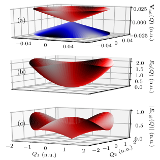
Figure 1: Potential energy surfaces in the cubic $E\otimes e$ model of the Jahn–Teller effect in NO₃ in the vicinity of the conical intersection at $Q=0$. (a) Elements $V_{1}(Q)=V_{+}(Q)$ (red) and $V_{2}(Q)=V_{-}(Q)$ (blue) of the diagonal adiabatic potential energy matrix; the two surfaces intersect (touch) at the point $Q=0$. The diabatic potential energy matrix consists of (b) the cubic potential energy surfaces $E_{0}(Q)$ on the diagonal and (c) the off-diagonal complex couplings of magnitude $|E_{\mathrm{cpl}}(Q)|$.

In the cubic Jahn–Teller model, the regularized diabatization scheme[45, 46, 47] can be implemented analytically. The $j$th-order adiabatic to quasidiabatic transformation matrix

$$\mathbf{S}(Q)=\frac{1}{\sqrt{2}}\begin{pmatrix}e^{-i\theta^{(j)}(Q)}&e^{-i\theta^{(j)}(Q)}\\ e^{i\theta^{(j)}(Q)}&-e^{i\theta^{(j)}(Q)}\end{pmatrix}$$ (24)

is obtained simply by replacing $\theta(Q)$ with $\theta^{(j)}(Q)$ in Eq. (20) for $\mathbf{T}(Q)$: $\theta^{(1)}(\rho,\phi):=\phi/2$ in the first-order scheme,

$$\theta^{(2)}(\rho,\phi):=\frac{1}{2}\arctan{\frac{c_{1}\rho\sin{\phi}-c_{2}\rho^{2}\sin{2\phi}}{c_{1}\rho\cos{\phi}+c_{2}\rho^{2}\cos{2\phi}}}$$ (25)

in the second-order scheme, while—in the cubic Jahn–Teller model—the third-order quasidiabatization is already identical to the strict diabatization, i.e., $\theta^{(3)}(\rho,\phi)=\theta(\rho,\phi)$. The quasidiabatization yields the potential energy matrix

$$\mathbf{V}_{\mathrm{qd}}(Q) :=\mathbf{S}(Q)\mathbf{V}_{\mathrm{ad}}(Q)\mathbf{S}(Q)^{\dagger}$$

$$=\begin{pmatrix}E_{0}(Q)&|E_{\mathrm{cpl}}(Q)|e^{-2i\theta^{(j)}(Q)}\\ |E_{\mathrm{cpl}}(Q)|e^{2i\theta^{(j)}(Q)}&E_{0}(Q)\end{pmatrix},$$ (26)

residual vector couplings

$$\mathbf{F}_{\mathrm{qd}}(Q) :=\mathbf{S}(Q)\mathbf{F}_{\mathrm{ad}}(Q)\mathbf{S}(Q)^{\dagger}+\mathbf{S}(Q)\nabla\mathbf{S}(Q)^{\dagger}$$

$$=-i\nabla\theta_{-}^{(j)}(Q)\begin{pmatrix}1&0\\ 0&-1\end{pmatrix},$$ (27)

and residual scalar couplings

$$\mathbf{G}_{\mathrm{qd}}(Q) :=\mathbf{S}(Q)\mathbf{G}_{\mathrm{ad}}(Q)\mathbf{S}(Q)^{\dagger}$$

$$+2 \mathbf{S}(Q)\mathbf{F}_{\mathrm{ad}}(Q)\nabla\mathbf{S}(Q)^{\dagger}+\mathbf{S}(Q)\nabla^{2}\mathbf{S}(Q)^{\dagger}$$

$$=-i\nabla^{2}\theta_{-}^{(j)}(Q)\begin{pmatrix}1&0\\ 0&-1\end{pmatrix}-[\nabla\theta_{-}^{(j)}(Q)]^{2}\begin{pmatrix}1&0\\ 0&1\end{pmatrix},$$ (28)

where $\theta_{-}^{(j)}(Q):=\theta(Q)-\theta^{(j)}(Q)$. The resulting magnitude of the residual couplings in the first-order ($j=1$) scheme is $\mathcal{R}[\mathbf{F}_{\mathrm{qd}}(Q)]=3.8$ n.u.

The hermiticity of Hamiltonian (9) is broken on a finite grid because the commutator relation $[\hat{P},\mathbf{F}_{\mathrm{qd}}(\hat{Q})]=-i\hbar\nabla\cdot\mathbf{F}_{\mathrm{qd}}(\hat{Q})$ holds only approximately unless the grid is infinitely dense. Yet, the hermiticity of the Hamiltonian is essential for the norm conservation (see Fig. S5 in Sec. S3 of the supplementary material), which, in turn, is required for quantum fidelity $\mathcal{F}(t)$ and distance $\mathcal{D}(t)$ to be valid measures of the importance of the residual nonadiabatic couplings. To make the exact quasidiabatic Hamiltonian exactly Hermitian, we re-express it as

$$\hat{\mathbf{H}}_{\text{qd-exact}}=\frac{1}{2M}[\hat{P}\mathbf{1}-i\hbar\mathbf{F}_{\mathrm{qd}}(\hat{Q})]^{2}+\mathbf{V}_{\mathrm{qd}}(\hat{Q}),$$ (29)

using the relationship

$$\mathbf{G}_{\mathrm{qd}}(Q)=\nabla\cdot\mathbf{F}_{\mathrm{qd}}(Q)+\mathbf{F}_{\mathrm{qd}}(Q)^{2},$$ (30)

which holds—exceptionally—for systems, such as the Jahn–Teller model, that can be represented exactly by a finite number of states; in general, Eq. (30) only holds when $S\rightarrow\infty$.

Another benefit of Hamiltonian (29) is the absence of $\mathbf{G}_{\mathrm{qd}}(Q)$, the evaluation of which represents the computational bottleneck in realistic systems. Likewise, the equations of motion in the widely-employed Meyer–Miller approach[95, 96, 97, 98] can be simplified greatly[72] by starting from Hamiltonian (29) instead of Hamiltonian (9). These two forms of the molecular Hamiltonian, however, are strictly equivalent only if the electronic basis is complete.[71, 21] In generic systems, in which the relation (30) does not hold and one is obliged to use the original Hamiltonian (9) and evaluate $\mathbf{G}_{\mathrm{qd}}(Q)$, the computationally expensive evaluation of the second derivatives of electronic wavefunctions with respect to nuclear coordinates can still be avoided by using the relation

$$\mathbf{G}_{\mathrm{qd}}(Q)=\nabla\cdot\mathbf{F}_{\mathrm{qd}}(Q)-\mathbf{K}_{\mathrm{qd}}(Q),$$ (31)

where $[\mathbf{K}_{\mathrm{qd}}(Q)]_{mn}:=\langle\nabla m^{\prime}(Q)|\nabla n^{\prime}(Q)\rangle$ requires only the first derivatives of the quasidiabatic electronic states $|n^{\prime}(Q)\rangle$, introduced in Eq. (8). In contrast to Eq. (30), relation (31) holds in arbitrary systems and for finite $S$.

To analyze the importance of residual couplings in NO₃, we simulated, with either the exact or approximate quasidiabatic Hamiltonian, the quantum dynamics following an electronic transition from the ground vibrational eigenstate of the ground electronic state $V_{\mathrm{g}}(Q)=-E_{\mathrm{gap}}+k\rho(Q)^{2}/2$ with $E_{\mathrm{gap}}=11$ n.u. ($1$ n.u. of energy here corresponds to $0.2$ eV $\approx 0.007$ a.u.). Invoking the time-dependent perturbation theory and Condon approximation, we considered the initial state in the quasidiabatic representation to be

$$\bm{\psi}(Q,t=0):=\frac{e^{-\rho(Q)^{2}/2\hbar}}{\sqrt{2\pi\hbar}}\begin{pmatrix}1\\ 1\end{pmatrix},$$ (32)

where we omitted (and will omit) the superscript “qd” on the wavepacket for brevity.

Figure 2 shows that, in the nonadiabatic dynamics following the vertical excitation of NO₃, neglecting the residual couplings does not significantly affect the wavepacket [compare panels (a) and (b)], power spectrum $I(\omega)$ [panel (c)], or population $\mathcal{P}_{1}^{\mathrm{ad}}(t)$ [panel (d)]. Even the fidelity $\mathcal{F}(t)$ [panel (e)] between the wavepackets propagated either with or without the residual couplings remains close to the maximal value of $1$ until the final time $t_{f}$. Section S4 of the supplementary material further supports this conclusion by displaying the time dependence of position $\langle\rho\rangle(t)$, potential energy $\langle\mathbf{V}_{\mathrm{qd}}\rangle(t)$, and distance $\mathcal{D}(t)$. In contrast, as we will see in Secs. III.2 and III.3, the residual couplings are much more significant in the HCN model and in the displaced excitation of NO₃.

In Sec. S5 of the supplementary material, we also analyze the importance of the residual couplings for different Jahn–Teller coupling coefficients and different initial populations.

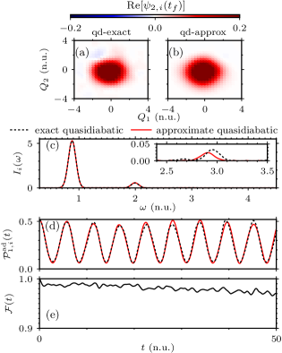
Figure 2: Importance of the residual nonadiabatic couplings in the NO₃ model from Sec. III.1. The figure compares the wavepackets and observables obtained with either the exact ($i=\textrm{qd-exact}$) or approximate ($i=\textrm{qd-approx}$) quasidiabatic Hamiltonian. (a) and (b): Wavepackets propagated with (a) $\hat{\mathbf{H}}_{\text{qd-exact}}$ from Eq. (9) and (b) $\hat{\mathbf{H}}_{\text{qd-approx}}$ from Eq. (13). [Only the real part of the nuclear wavepacket in the second ($n=2$) electronic state is shown.] (c) Power spectrum $I_{i}(\omega)$ obtained by Fourier transforming the damped autocorrelation function. [To emulate the broadening of the spectral peaks, the autocorrelation function $C_{i}(t)=\langle\bm{\psi}(0)|\bm{\psi}_{i}(t)\rangle$ was multiplied by the damping function $d(t)=\exp[(-t/t_{\mathrm{damp}})^{2}]$ with $t_{\mathrm{damp}}=17.5$ n.u.] (d) Population $\mathcal{P}_{1,i}^{\mathrm{ad}}(t):=\langle\bm{\psi}_{i}^{\mathrm{ad}}(t)|\mathbf{P}_{1}|\bm{\psi}_{i}^{\mathrm{ad}}(t)\rangle$ of the first ($n=1$) adiabatic electronic state; $\mathbf{P}_{n}:=|n\rangle\langle n|$ is the population operator of the $n$th adiabatic state. (e) Errors due to ignoring the residual couplings are measured by quantum fidelity $\mathcal{F}(t)$ [Eq. (14)].

III.2 Induced Renner–Teller effect in hydrogen cyanide

The model of the induced Renner–Teller effect[41, 67, 68, 69] is more realistic than the Jahn–Teller model from Sec. III.1: In particular, the strictly diabatic Hamiltonian (16) cannot be defined and relationship (30) does not hold. Nevertheless, similarly to the Jahn–Teller model, the nonadiabatic couplings between the adiabatic states are singular at $Q=0$.[41] Since Eq. (30) does not hold in the induced Renner–Teller model, the exactly Hermitian Hamiltonian (29) cannot be used instead of Hamiltonian (9). Yet, even with Hamiltonian (9), the norm is sufficiently converged in grid density for the quantum fidelity $\mathcal{F}(t)$ and distance $\mathcal{D}(t)$ to be valid (see Fig. S6 of the supplementary material).

We follow Ref. 41, where the induced Renner–Teller model is quasidiabatized with the block-diagonalization scheme, which minimizes the residual couplings locally (around $Q=0$ in this model).[21] The resulting quasidiabatic potential energy matrix

$$\mathbf{V}_{\mathrm{qd}}(\rho,\phi)=\begin{pmatrix}V_{+}(\rho)&V_{-}(\rho)e^{-2i\phi}\\ V_{-}(\rho)e^{2i\phi}&V_{+}(\rho)\end{pmatrix}$$ (33)

with $V_{\pm}(\rho):=[V_{1}(\rho)\pm V_{2}(\rho)]/2$ depends on the adiabatic potential energy surfaces $V_{1}(\rho)=\Delta+E_{\mathrm{h}}(\rho)-w(\rho)$ and $V_{2}(\rho)=E_{\mathrm{h}}(\rho)$, where $E_{\mathrm{h}}(\rho):=k\rho^{2}/2$ and $w(\rho):=(\Delta^{2}+2\lambda^{2}\rho^{2})^{1/2}$. Analytical expressions for the nonadiabatic couplings, $\mathbf{F}_{\mathrm{ad}}(Q)$ and $\mathbf{G}_{\mathrm{ad}}(Q)$, and adiabatic to quasidiabatic transformation matrix $\mathbf{S}(Q)$ can be found in Ref. 41. In our nonadiabatic simulations of hydrogen cyanide, we used the induced Renner–Teller model of HCN from Refs. 41, 67 with parameters $\Delta=1.11$ n.u. and $\lambda=1$ n.u. The residual vector and scalar couplings[41] are, respectively,

$$\mathbf{F}_{\mathrm{qd}}(Q)=iv_{F}(Q)\begin{pmatrix}1&0\\ 0&-1\end{pmatrix}$$ (34)

and

$$\mathbf{G}_{\mathrm{qd}}(\rho,\phi)=2\begin{pmatrix}f_{F}(\rho)-f_{G}(\rho)&-f_{G}(\rho)e^{-2i\phi}\\ -f_{G}(\rho)e^{2i\phi}&f_{F}(\rho)-f_{G}(\rho)\end{pmatrix},$$ (35)

where we have defined the $D$-dimensional (here $D=2$) vector $v_{F}(Q)$ with components $v_{F}(Q)_{1}=-f_{F}(\rho(Q))Q_{2}$ and $v_{F}(Q)_{2}=f_{F}(\rho(Q))Q_{1},$ and functions $f_{F}(\rho):=[1-w_{+}(\rho)]/\rho^{2}$ and

$$f_{G}(\rho):=\left[\frac{w_{-}(\rho)}{2\rho}\right]^{2}-\left[\frac{\lambda}{2\sqrt{2}w(\rho)}\right]^{2}+\left[\frac{\lambda^{2}\rho}{2w(\rho)^{2}}\right]^{2}$$ (36)

with $w_{\pm}(\rho):=\sqrt{[1\pm\Delta/w(\rho)]/2}$. The magnitude of the residual couplings (34) is $\mathcal{R}[\mathbf{F}_{\mathrm{qd}}(Q)]=0.37$ n.u.; the adiabatic potential energy surfaces and functions $f_{F}$ and $f_{G}$ are plotted in Fig. 3.

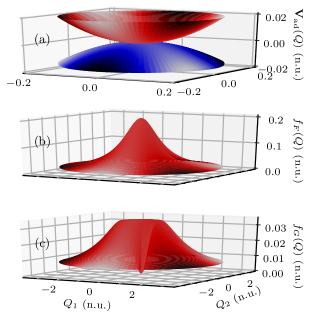
Figure 3: Potential energy surfaces in the model of the induced Renner–Teller effect in HCN in the vicinity of the Renner–Teller intersection at $Q=0$. (a) The two adiabatic potential energy surfaces $V_{1}(Q)$ (blue) and $V_{2}(Q)$ (red) intersect (touch) at the point $Q=0$. The residual couplings (34) and (35) depend on plotted functions $f_{F}(Q)$ [panel (b)] and $f_{G}(Q)$ [panel (c)].

Similarly to Sec. III.1, we simulate the dynamics following an electronic transition from the ground vibrational eigenstate of $V_{\mathrm{g}}(\rho,\phi)=-E_{\mathrm{gap}}+E_{\mathrm{h}}(\rho)$ with $E_{\mathrm{gap}}=153$ n.u. ($1$ n.u. of energy here corresponds to $0.09$ eV $\approx 0.003$ a.u.). Unlike their analogues in Sec. III.1, however, the two wavepackets, propagated with either the exact or approximate quasidiabatic Hamiltonian, differ significantly [compare panels (a) and (b) of Fig. 4]. Ignoring the residual couplings also leads to large errors in the power spectrum $I(\omega)$ [panel (c)], population $\mathcal{P}_{1}^{\mathrm{ad}}(t)$ [panel (d)], and fast decay of quantum fidelity $\mathcal{F}(t)$ [panel (e)]. In particular, the population obtained with the approximate quasidiabatic Hamiltonian cannot be trusted because, e.g., at $t=169$ n.u., the error $\epsilon_{\text{res-cpl}}[\mathcal{P}_{1}^{\mathrm{ad}}(t)]:=|\mathcal{P}_{1,\text{qd-approx}}^{\mathrm{ad}}(t)-\mathcal{P}_{1,\text{qd-exact}}^{\mathrm{ad}}(t)|$ due to the neglect of the residual couplings is of the same order as the range $R_{\mathcal{P}_{1}^{\mathrm{ad}}}:=\mathcal{P}_{1,\mathrm{max}}^{\mathrm{ad}}-\mathcal{P}_{1,\mathrm{min}}^{\mathrm{ad}}$ of the population in the whole simulation interval: $\epsilon_{\text{res-cpl}}[\mathcal{P}_{1}^{\mathrm{ad}}(t)]/R_{\mathcal{P}_{1}^{\mathrm{ad}}}=0.7$. Note also that neither $\mathcal{P}_{1}^{\mathrm{ad}}(t)$ nor $\mathcal{F}(t)$ is affected by the overall phases of the two wavepackets, although a linearly growing overall phase difference appears to be the main contribution to the change of the spectrum, which is mostly shifted [see panel (c) of Fig. 4].

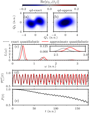
Figure 4: Importance of the residual nonadiabatic couplings in the HCN model from Sec. III.2. (a) and (b): wavepackets, (c) power spectrum, (d) population, (e) fidelity. See the caption of Fig. 2 for a detailed description of the content of the five panels.

III.3 Displaced excitation of nitrogen trioxide

Although the excited states of NO₃ from Sec. III.1 are bright states, the coupled states modeled by the cubic $E\otimes e$ Jahn–Teller Hamiltonian can sometimes be dark. A wavepacket might reach such dark states at a nuclear geometry that is not the ground state equilibrium (e.g., via an intersection with a bright state). Motivated by this observation from Ref. 64, we consider the initial state (32) displaced in both $Q_{1}$ and $Q_{2}$ by $-0.8$ n.u. Keeping all other parameters fixed as in Sec. III.1 will allow us to analyze how the importance of the residual couplings depends on the initial state and on the quasidiabatization method used.

Figure 5 shows that, in contrast to the vertical excitation from Sec. III.1 (analyzed in Fig. 2), ignoring the residual couplings obtained by applying the first-order regularized scheme to the displaced excitation of NO₃ affects both the wavepacket [compare panels (a) and (b)] and observables significantly. Neither the spectrum $I(\omega)$ [panel (c)] nor population $\mathcal{P}_{1}^{\mathrm{ad}}(t)$ [panel (d)] is obtained accurately with the approximate quasidiabatic Hamiltonian. For example, at $t=25$ n.u., the error of the population is almost half of the range of the population in the whole simulation interval: $\epsilon_{\text{res-cpl}}[\mathcal{P}_{1}^{\mathrm{ad}}(t)]/R_{\mathcal{P}_{1}^{\mathrm{ad}}}=0.4$. The quantum fidelity [panel (e)] decreases rapidly to $\mathcal{F}(t_{f})\approx 0.3$ at $t_{f}=50$ n.u.

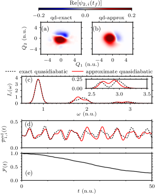
Figure 5: Importance of the residual nonadiabatic couplings in the model of a displaced excitation of NO₃ from Sec III.3. As in Fig. 2, the molecular Hamiltonian was quasidiabatized with the first-order ($j=1$) scheme. (a) and (b): wavepackets, (c) power spectrum, (d) population, (e) fidelity. See the caption of Fig. 2 for a detailed description of the content of the five panels.

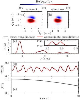
Figure 6: Importance of the residual nonadiabatic couplings in the model of a displaced excitation of NO₃ from Sec III.3. The only difference from Fig. 5 is that the molecular Hamiltonian was quasidiabatized with the second-order ($j=2$) scheme. (a) and (b): wavepackets, (c) power spectrum, (d) population, (e) fidelity. See the caption of Fig. 2 for a detailed description of the content of the five panels.

The residual couplings, however, can be made less important by an improved quasidiabatization. One can reduce the magnitude of the residual couplings from $\mathcal{R}[\mathbf{F}_{\mathrm{qd}}^{(1)}(Q)]=3.8$ n.u. to $\mathcal{R}[\mathbf{F}_{\mathrm{qd}}^{(2)}(Q)]=0.5$ n.u. by employing the more sophisticated, second-order regularized diabatization scheme[45, 46, 47] obtained by inserting $\theta^{(2)}(Q)$ from Eq. (25) in Eqs. (24) and (26)–(28). When this second-order scheme is used, the errors of the wavepacket $\bm{\psi}(t)$, spectrum $I(\omega)$, and population $\mathcal{P}_{1}^{\mathrm{ad}}(t)$ due to the neglect of the residual couplings all remain small (see Fig. 6); in particular, quantum fidelity $\mathcal{F}(t)$ remains above $0.95$ for all times until the final time $t_{f}=50$ n.u. [see panel (e)]. (Note that the exact benchmark wavepackets [in panels (a) of Figs. 5 and 6] propagated in the two different quasidiabatic representations are slightly different not only because they are displayed in different representations but also because the initial states are different—they have the same analytical form but in two different quasidiabatic representations.)

IV Conclusion

We have shown that the common practice of neglecting the residual nonadiabatic couplings between quasidiabatic states can substantially lower the accuracy of nonadiabatic simulations and that the decrease of accuracy depends on the system, initial state, and employed quasidiabatization scheme. One can, therefore, answer the question posed in the title only after a careful analysis. In Sec. III, we have provided several examples where the approximate quasidiabatic Hamiltonian gives wrong results. Because it is potentially dangerous to employ an approximation without evaluating its impact, we have proposed a method to rigorously quantify the errors caused by ignoring the residual couplings.

When the residual couplings are significant and cannot be neglected, we suggest performing nonadiabatic simulations with the rarely used exact quasidiabatic Hamiltonian (9), which not only is analytically equivalent to the adiabatic Hamiltonian (6), but also yields numerically accurate results regardless of the magnitude of the residual couplings (as shown in Sec. S2 of the supplementary material and in Ref. 49). Although the general applicability of the exact quasidiabatic Hamiltonian depends on the availability of residual nonadiabatic couplings, these can be evaluated by employing recently developed schemes[99, 100, 101, 102, 103] even in rather complicated multi-state systems involving multiple conical intersections (including those between three electronic states[104, 105, 106, 107, 108]). In complex systems where all practical quasidiabatization schemes lead to significant residual couplings, propagating the wavepacket with the exact quasidiabatic Hamiltonian would be particularly beneficial. Although the nonseparable form of this Hamiltonian complicates the time propagation, there exist efficient geometric integrators, such as the high-order compositions of the implicit midpoint method used here, which are applicable even to such Hamiltonians.

Last but not least, an accurate propagation of the wavepacket with the exact quasidiabatic Hamiltonian would be extremely useful for establishing highly accurate benchmarks in unfamiliar systems, where the impact of the residual nonadiabatic couplings on the quantum dynamics simulations is not yet known.

Supplementary material

See the supplementary material for the details of the numerical evaluation of the magnitude of the residual couplings (Sec. S1); demonstration of the negligibility of spatial and time discretization errors (Sec. S2); conservation of geometric properties by the implicit midpoint method (Sec. S3); time dependence of position, potential energy, and distance (Sec. S4); and importance of the residual couplings for different Jahn–Teller coupling coefficients and different initial populations (Sec. S5).

Data Availability

The data that support the findings of this study are contained in the paper and the supplementary material.

Supplementary material for: How important are the residual nonadiabatic couplings for an accurate simulation of nonadiabatic quantum dynamics in a quasidiabatic representation?

S1 Numerical evaluation of the magnitude of the residual couplings

The evaluation of the magnitude $\mathcal{R}[\mathbf{F}_{\mathrm{qd}}(Q)]$ of residual couplings requires an integration over the entire nuclear space [see Eq. (10) of the main text]. In the main text, we approximate the integral numerically on a finite grid of $N\times N$ points between $-Q_{l}$ and $Q_{l}$ for $l\in\{1,2\}$. In the nonadiabatic simulations, we used $N=64$ and $Q_{l}=10$ n.u. in the NO₃ model and $N=32$ and $Q_{l}=7$ n.u. in the HCN model.

To evaluate the magnitude $\mathcal{R}[\mathbf{F}_{\mathrm{qd}}(Q)]$ of the residual nonadiabatic couplings, we have chosen a grid narrower than the one used for nonadiabatic simulations because $\mathcal{R}[\mathbf{F}_{\mathrm{qd}}(Q)]$ evaluated on a wider grid would not be informative, as can be seen from the following consideration: In addition to the central conical intersection (at $Q=0$), the cubic Jahn–Teller model has six other conical intersections at $\rho(Q)=\rho_{+}$ and $\phi(Q)=-2\pi/3,0,2\pi/3$ and at $\rho(Q)=\rho_{-}$ and $\phi(Q)=-\pi/3,\pi/3,\pi$, where $\rho_{\pm}=(c_{2}\pm\sqrt{c_{2}^{2}-4c_{1}c_{3}})/(2c_{3})$. Although the singularities of the nonadiabatic couplings at these additional conical intersections remain even after the quasidiabatization by the regularized diabatization scheme, these singularities are sufficiently far from the region of the dynamics and do not have a significant effect on the simulations (i.e., numerical convergence was achieved despite the remaining singularities; see Sec. S2 of the supplementary material). However, because it diverges to infinity, the magnitude $\mathcal{R}[\mathbf{F}_{\mathrm{qd}}(Q)]$ of the residual couplings evaluated on a grid that includes these additional conical intersections is not meaningful. We, therefore, evaluate $\mathcal{R}[\mathbf{F}_{\mathrm{qd}}(Q)]$ on a narrower grid that does not include these singular residual couplings.

S2 Negligibility of spatial and time discretization errors

For the results presented in the main text to be valid, both the spatial and time discretization errors should be smaller than the errors due to the neglect of the residual nonadiabatic couplings. We used distance functionals $\epsilon_{N}^{(\mathrm{grid})}[\bm{\psi}(t)]:=\|\bm{\psi}^{(\Delta t,N)}(t)-\bm{\psi}^{(\Delta t,2N)}(t)\|$ and $\epsilon_{\Delta t}^{(\mathrm{time})}[\bm{\psi}(t)]:=\|\bm{\psi}^{(\Delta t,N)}(t)-\bm{\psi}^{(\Delta t/2,N)}(t)\|$ to measure the spatial and time discretization errors of $\bm{\psi}^{(\Delta t,N)}(t)$, the molecular wavepacket propagated to time $t$ with the time step of $\Delta t$ on a grid of $N\times N$ points. Similarly, we used $\epsilon_{N}^{(\mathrm{grid})}(A):=|A^{(\Delta t,N)}-A^{(\Delta t,2N)}|$ and $\epsilon_{\Delta t}^{(\mathrm{time})}(A):=|A^{(\Delta t,N)}-A^{(\Delta t/2,N)}|$ to measure the spatial and time discretization errors of $A^{(\Delta t,N)}$, an observable $A$ obtained from a simulation on a grid of $N\times N$ points with the time step $\Delta t$. The grid of $2N\times 2N$ points was defined so that it was both denser and wider by a factor of $\sqrt{2}$ (both in position and momentum spaces) compared to the grid of $N\times N$ points.

Figures S1–S4 show that the grid discretization errors of the quantities presented in the main text are smaller than the errors due to the neglect of the residual couplings. Moreover, thanks to the high order of accuracy of the employed time propagation scheme, the time discretization errors are negligible in comparison with the corresponding spatial discretization errors. The small numerical errors of the wavepackets propagated with the exact quasidiabatic Hamiltonian validate them as the reference benchmark wavepackets because the exact quasidiabatic Hamiltonian is exact in the sense that it is a coordinate-dependent unitary transform of the adiabatic Hamiltonian.

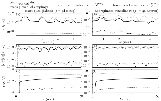
Figure S1: Negligibility of spatial and time discretization errors of the quantities presented in Fig. 2 of the main text: (a)–(b) power spectrum $I_{i}(\omega)$, (c)–(d) population $\mathcal{P}_{1,i}^{\mathrm{ad}}(t)$, and (e)–(f) wavepacket $\bm{\psi}_{i}(t)$ obtained with either the exact [$i=\textrm{qd-exact}$, panels (a), (c), (e)] or approximate [$i=\textrm{qd-approx}$, panels (b), (d), (f)] Hamiltonian. In each panel, errors $\epsilon_{\textrm{res-cpl}}$ due to the neglect of the residual couplings are compared with the grid discretization errors $\epsilon_{N}^{\mathrm{(grid)}}$ and time discretization errors $\epsilon_{\Delta t}^{\mathrm{(time)}}$. Note that $\epsilon_{\textrm{res-cpl}}[\bm{\psi}(t)]\equiv\mathcal{D}(t):=\|\bm{\psi}_{\textrm{qd-approx}}(t)-\bm{\psi}_{\textrm{qd-exact}}(t)\|$.

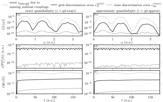
Figure S2: Negligibility of spatial and time discretization errors of the quantities presented in Fig. 4 of the main text. See the caption of Fig. S1 for details.

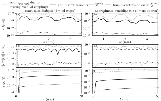
Figure S3: Negligibility of spatial and time discretization errors of the quantities presented in Fig. 5 of the main text. See the caption of Fig. S1 for details.

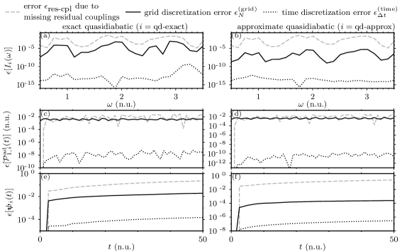
Figure S4: Negligibility of spatial and time discretization errors of the quantities presented in Fig. 6 of the main text. See the caption of Fig. S1 for details.

S3 Conservation of geometric properties by the implicit midpoint method

Here, we demonstrate the exact conservation of the wavepacket’s norm $\|\bm{\psi}(t)\|$ and energy $\langle E(t)\rangle$ by the optimal eighth-order[58] composition[59, 60, 57, 61] of the implicit midpoint method. Figure S5 shows that both the norm and energy are conserved to machine precision ($<10^{-12}$) in the model of vertical excitation of NO₃ from Sec. III A of the main text. In fact, they are conserved to machine precision regardless of the size of the time step (not shown). We refer the reader to Ref. 54 and the references therein for the analytical proof and numerical demonstration of the preservation of geometric properties of the exact solution (the conservation of norm, energy, and inner-product, linearity, symplecticity, stability, symmetry, and time reversibility) by the compositions of the implicit midpoint method.

Figure S6 shows the norm and energy conservation in the HCN model from Sec. III B of the main text. Note that here the norm is not conserved to machine precision, but “only” to $10^{-8}$; the subtle reason for this effect is that on a finite grid, the exact quasidiabatic Hamiltonian (9) of the main text is only approximately Hermitian. In contrast, simulations with exactly Hermitian Hamiltonians [e.g., Hamiltonians (12) and (28) of the main text] conserve the norm and energy exactly regardless of the grid density (not shown).

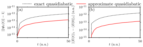
Figure S5: Exact conservation of geometric properties in the vertical excitation of NO₃ (from Sec. III A of the main text) by the employed integrator: the conservation of the (a) norm $\|\bm{\psi}_{i}(t)\|$ and (b) energy $\langle E(t)\rangle_{i}$ of the wavepacket propagated with either the exact ($i=\textrm{qd-exact}$) or approximate ($i=\textrm{qd-approx}$) quasidiabatic Hamiltonian. The initial values are $\|\bm{\psi}_{i}(0)\|=1$ and $\langle E(0)\rangle_{i}=1$ n.u.

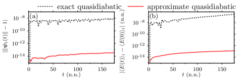
Figure S6: Exact conservation of geometric properties in the HCN model (from Sec. III B of the main text) by the employed integrator. See the caption of Fig. S5 for details. Here, the initial norm is $\|\bm{\psi}_{i}(0)\|=1$ and the initial energies are $\langle E(0)\rangle_{\textrm{qd-exact}}=0.6$ n.u. and $\langle E(0)\rangle_{\textrm{qd-approx}}=0.7$ n.u.

S4 Time dependence of position, potential energy, and distance

To supplement Figs. 2, 4–6 of the main text, we present, in Figs. S7–S10, the time dependence of the position $\langle\rho\rangle_{i}(t):=[\sum_{l=1}^{2}\langle\bm{\psi}_{i}(t)|\hat{Q}_{l}|\bm{\psi}_{i}(t)\rangle^{2}]^{1/2}$ [panels (a)] and potential energy $\langle\mathbf{V}_{\mathrm{qd}}\rangle_{i}(t):=\langle\bm{\psi}_{i}(t)|\mathbf{V}_{\mathrm{qd}}(\hat{Q})|\bm{\psi}_{i}(t)\rangle$ [panels (b)] obtained either with the approximate ($i=\text{qd-approx}$) or exact ($i=\text{qd-exact}$) quasidiabatic Hamiltonian. In panels (c), we show the distance

$$\mathcal{D}(t):=\|\bm{\psi}_{\text{qd-approx}}(t)-\bm{\psi}_{\text{qd-exact}}(t)\|$$ (S1)

between the wavepackets propagated either with the approximate or exact Hamiltonian.

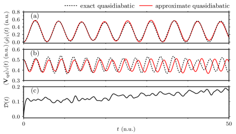
Figure S7: Importance of the residual nonadiabatic couplings in the NO₃ model from Sec. III A of the main text. The figure, which complements Fig. 2 of the main text, shows the time dependence of (a) position $\langle\rho\rangle_{i}(t)$, (b) potential energy $\langle\mathbf{V}_{\mathrm{qd}}\rangle_{i}(t)$, and (c) distance $\mathcal{D}(t)$ [Eq. (S1)].

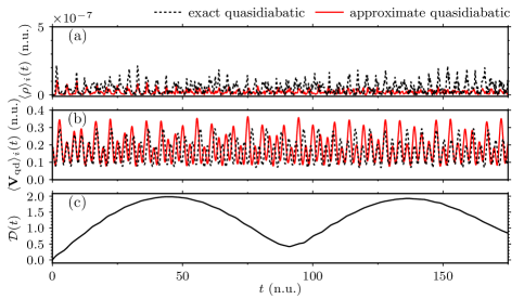
Figure S8: Importance of the residual nonadiabatic couplings in the HCN model from Sec. III B of the main text. The figure, which complements Fig. 4 of the main text, shows the time dependence of (a) position $\langle\rho\rangle_{i}(t)$, (b) potential energy $\langle\mathbf{V}_{\mathrm{qd}}\rangle_{i}(t)$, and (c) distance $\mathcal{D}(t)$ [Eq. (S1)]. Note that the wavepacket remains at $\langle\rho\rangle_{i}(t)=0$ throughout the dynamics and only its width changes (not shown).

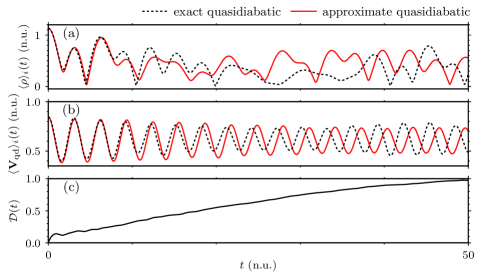
Figure S9: Importance of the residual nonadiabatic couplings in the model of a displaced excitation of NO₃ from Sec. III C of the main text. The molecular Hamiltonian was quasidiabatized with the first-order ($j=1$) scheme. The figure, which complements Fig. 5 of the main text, shows the time dependence of (a) position $\langle\rho\rangle_{i}(t)$, (b) potential energy $\langle\mathbf{V}_{\mathrm{qd}}\rangle_{i}(t)$, and (c) distance $\mathcal{D}(t)$ [Eq. (S1)].

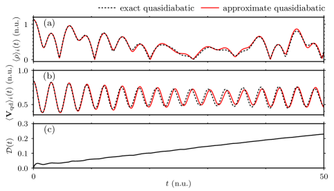
Figure S10: Importance of the residual nonadiabatic couplings in the model of a displaced excitation of NO₃ from Sec. III C of the main text. The molecular Hamiltonian was quasidiabatized with the second-order ($j=2$) scheme. The figure, which complements Fig. 6 of the main text, shows the time dependence of (a) position $\langle\rho\rangle_{i}(t)$, (b) potential energy $\langle\mathbf{V}_{\mathrm{qd}}\rangle_{i}(t)$, and (c) distance $\mathcal{D}(t)$ [Eq. (S1)].

S5 Importance of the residual couplings for different Jahn–Teller coupling coefficients and different initial populations

In Fig. S11(a), we consider four sets of Jahn–Teller coupling coefficients, represented by triples $C=(c_{1},c_{2},c_{3})$ [all in natural units (n.u.)]: $C_{1}=(0.375,-0.0668,0.0119)$, $C_{2}=(0.375,-0.05,-0.0155)$, $C_{3}=(0.375,-0.037,-0.0185)$, and $C_{4}=(1.5,0.388,0.052)$. Among these, triple $C_{1}$ consists of the coefficients of the NO₃ model discussed in Sec. III C of the main text. The other triples were chosen so that the magnitudes of the residual couplings in the first-order quasidiabatization were $\mathcal{R}[\mathbf{F}_{\mathrm{qd}}(Q)]=3.8$ n.u. for both $C_{1}$ and $C_{4}$, $\mathcal{R}[\mathbf{F}_{\mathrm{qd}}(Q)]=2.4$ n.u. for $C_{2}$, and $\mathcal{R}[\mathbf{F}_{\mathrm{qd}}(Q)]=1.6$ n.u. for $C_{3}$ and so that $\mathcal{R}[\mathbf{F}_{\mathrm{qd}}(Q)]=0.5$ n.u. for all four triples if the second-order scheme was employed. Because the triples $C_{1}$, $C_{2}$, and $C_{3}$ are similar, the resulting nonadiabatic dynamics were also similar; in contrast, the dynamics with triple $C_{4}$ was very different (not shown). On one hand, panel (a) of Fig. S11 shows that there is a positive correlation between the magnitude and importance of the residual couplings when the dynamics are similar. On the other hand, even when the magnitudes $\mathcal{R}[\mathbf{F}_{\mathrm{qd}}(Q)]$ are the same, the importance of residual couplings can differ significantly if the nonadiabatic dynamics are not the same (compare the results for $C_{1}$ and $C_{4}$).

In panel (b), we consider three different initial states that only differed in the initial quasidiabatic populations: the population of the first state was $\mathcal{P}_{1}(0)=0.5$, $0.9$, or $0.1$; in all cases, $\mathcal{P}_{2}(0)=1-\mathcal{P}_{1}(0)$. The initial state with $\mathcal{P}_{1}(0)=0.5$ was the one analyzed in Sec. III C of the main text. Panel (b) of Fig. S11 shows that, in the case of the displaced excitation of NO₃, the importance of the residual couplings is almost independent of the distribution of the initial populations among the different states. This conclusion, however, may not apply to other systems.

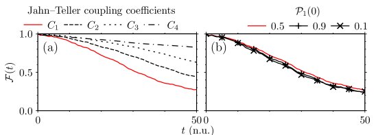
Figure S11: Importance of the residual couplings in the displaced excitation of NO₃ (from Sec. III C of the main text) for (a) different Jahn–Teller coupling coefficients and (b) different initial quasidiabatic populations $\mathcal{P}_{1}(0)$. The importance of the residual couplings is measured by quantum fidelity [as in Fig. 5(e) of the main text] and shown only for the first-order quasidiabatization scheme. Results based on the second-order quasidiabatization scheme are not shown since they are very accurate [i.e., $\mathcal{F}(t)\approx 1$] in all presented cases. The red solid lines in the two panels are identical to each other and to the black solid line in Fig. 5(e) of the main text.

References

- Born and Oppenheimer [1927] M. Born and R. Oppenheimer, Ann. d. Phys. 389, 457 (1927).
- Domcke and Yarkony [2012] W. Domcke and D. R. Yarkony, Annu. Rev. Phys. Chem. 63, 325 (2012).
- Nakamura [2012] H. Nakamura, Nonadiabatic Transition: Concepts, Basic Theories and Applications, 2nd ed. (World Scientific Publishing Company, 2012).
- Takatsuka et al. [2015] K. Takatsuka, T. Yonehara, K. Hanasaki, and Y. Arasaki, Chemical Theory Beyond the Born-Oppenheimer Paradigm: Nonadiabatic Electronic and Nuclear Dynamics in Chemical Reactions (World Scientific, Singapore, 2015).
- Bircher et al. [2017] M. P. Bircher, E. Liberatore, N. J. Browning, S. Brickel, C. Hofmann, A. Patoz, O. T. Unke, T. Zimmermann, M. Chergui, P. Hamm, U. Keller, M. Meuwly, H. J. Woerner, J. Vaníček, and U. Rothlisberger, Struct. Dyn. 4, 061510 (2017).
- Shin and Metiu [1995] S. Shin and H. Metiu, J. Chem. Phys. 102, 9285 (1995).
- Albert, Kaiser, and Engel [2016] J. Albert, D. Kaiser, and V. Engel, J. Chem. Phys. 144, 171103 (2016).
- Abedi, Maitra, and Gross [2010] A. Abedi, N. T. Maitra, and E. K. Gross, Phys. Rev. Lett. 105, 123002 (2010).
- Cederbaum [2008] L. S. Cederbaum, J. Chem. Phys. 128, 124101 (2008).
- Zimmermann and Vaníček [2010] T. Zimmermann and J. Vaníček, J. Chem. Phys. 132, 241101 (2010).
- Zimmermann and Vaníček [2012] T. Zimmermann and J. Vaníček, J. Chem. Phys. 136, 094106 (2012).
- Worth and Cederbaum [2004] G. A. Worth and L. S. Cederbaum, Annu. Rev. Phys. Chem. 55, 127 (2004).
- Baer [2006] M. Baer, Beyond Born-Oppenheimer: Electronic Nonadiabatic Coupling Terms and Conical Intersections, 1st ed. (Wiley, 2006).
- Cederbaum [2004] L. S. Cederbaum, in Conical Intersections: Electronic Structure, Dynamics and Spectroscopy (World Scientific, 2004) pp. 3–40.
- Teller [1937] E. Teller, J. Phys. Chem. 41, 109 (1937).
- Herzberg and Longuet-Higgins [1963] G. Herzberg and H. C. Longuet-Higgins, Faraday Discuss. 35, 77 (1963).
- Zimmerman [1966] H. E. Zimmerman, J. Am. Chem. Soc. 88, 1566 (1966).
- Förster [1970] T. Förster, Pure Appl. Chem 24, 443 (1970).
- Yarkony [2004] D. R. Yarkony, in Conical intersections: electronic structure, dynamics and spectroscopy (World Scientific, 2004) pp. 41–127.
- Köppel [2004] H. Köppel, in Conical intersections: electronic structure, dynamics and spectroscopy (World Scientific, 2004) pp. 175–204.
- Pacher et al. [1989] T. Pacher, C. A. Mead, L. S. Cederbaum, and H. Köppel, J. Chem. Phys. 91, 7057 (1989).
- Pacher, Cederbaum, and Köppel [1993] T. Pacher, L. S. Cederbaum, and H. Köppel, Advances in Chemical Physics 84, 293 (1993).
- Baer [1975] M. Baer, Chem. Phys. Lett. 35, 112 (1975).
- Das et al. [2011] A. Das, D. Mukhopadhyay, S. Adhikari, and M. Baer, Chemical Physics Letters 517, 92 (2011).
- Richings and Worth [2015] G. W. Richings and G. A. Worth, J. Phys. Chem. A 119, 12457 (2015).
- Sadygov and Yarkony [1998] R. G. Sadygov and D. R. Yarkony, J. Chem. Phys. 109, 20 (1998).
- Esry and Sadeghpour [2003] B. D. Esry and H. R. Sadeghpour, Phys. Rev. A 68, 042706 (2003).
- Evenhuis and Collins [2004] C. R. Evenhuis and M. A. Collins, J. Chem. Phys. 121, 2515 (2004).
- Guan, Guo, and Yarkony [2019] Y. Guan, H. Guo, and D. R. Yarkony, J. Chem. Phys. 150, 214101 (2019).
- Malbon and Yarkony [2015] C. L. Malbon and D. R. Yarkony, J. Phys. Chem. A 119, 7498 (2015).
- Zhu and Yarkony [2010] X. Zhu and D. R. Yarkony, J. Chem. Phys. 132, 104101 (2010).
- Zhu and Yarkony [2012a] X. Zhu and D. R. Yarkony, J. Chem. Phys. 136, 174110 (2012a).
- Zhu and Yarkony [2016a] X. Zhu and D. R. Yarkony, Mol. Phys. 114, 1983 (2016a).
- Mulliken [1952] R. S. Mulliken, J. Am. Chem. Soc. 74, 811 (1952).
- Hush [1967] N. S. Hush, Prog. Inorg. Chem 8, 391 (1967).
- Cave and Newton [1997] R. J. Cave and M. D. Newton, J. Chem. Phys. 106, 9213 (1997).
- Werner and Meyer [1981] H. Werner and W. Meyer, J. Chem. Phys. 74, 5802 (1981).
- Yarkony [1998] D. R. Yarkony, J. Phys. Chem. A 102, 8073 (1998).
- Hirsch, Buenker, and Petrongolo [1990] G. Hirsch, R. J. Buenker, and C. Petrongolo, Molecular Physics 70, 835 (1990).
- Perić, Peyerimhoff, and Buenker [1990] M. Perić, S. D. Peyerimhoff, and R. J. Buenker, Molecular Physics 71, 693 (1990).
- Pacher, Cederbaum, and Köppel [1988] T. Pacher, L. S. Cederbaum, and H. Köppel, J. Chem. Phys. 89, 7367 (1988).
- Pacher, Köppel, and Cederbaum [1991] T. Pacher, H. Köppel, and L. S. Cederbaum, J. Chem. Phys. 95, 6668 (1991).
- Neville, Seidu, and Schuurman [2020] S. P. Neville, I. Seidu, and M. S. Schuurman, J. Chem. Phys. 152, 114110 (2020).
- Domcke and Woywod [1993] W. Domcke and C. Woywod, Chem. Phys. Lett. 216, 362 (1993).
- Thiel and Köppel [1999] A. Thiel and H. Köppel, J. Chem. Phys. 110, 9371 (1999).
- Köppel, Gronki, and Mahapatra [2001] H. Köppel, J. Gronki, and S. Mahapatra, J. Chem. Phys. 115, 2377 (2001).
- Köppel and Schubert [2006] H. Köppel and B. Schubert, Mol. Phys. 104, 1069 (2006).
- Mead and Truhlar [1982] C. A. Mead and D. G. Truhlar, J. Chem. Phys. 77, 6090 (1982).
- Choi and Vaníček [2020] S. Choi and J. Vaníček, J. Chem. Phys. 153, 211101 (2020).
- Tal-Ezer and Kosloff [1984] H. Tal-Ezer and R. Kosloff, J. Chem. Phys. 81, 3967 (1984).
- Lanczos [1950] C. Lanczos, J. Res. Nat. Bur. Stand. 45, 255 (1950).
- Tal-Ezer [1989] H. Tal-Ezer, J. Sci. Comput. 4, 25 (1989).
- Park and Light [1986] T. J. Park and J. C. Light, J. Chem. Phys. 85, 5870 (1986).
- Choi and Vaníček [2019] S. Choi and J. Vaníček, J. Chem. Phys. 150, 204112 (2019).
- Leforestier et al. [1991] C. Leforestier, R. H. Bisseling, C. Cerjan, M. D. Feit, R. Friesner, A. Guldberg, A. Hammerich, G. Jolicard, W. Karrlein, H.-D. Meyer, N. Lipkin, O. Roncero, and R. Kosloff, J. Comp. Phys. 94, 59 (1991).
- Leimkuhler and Reich [2004] B. Leimkuhler and S. Reich, Simulating Hamiltonian Dynamics (Cambridge University Press, 2004).
- Hairer, Lubich, and Wanner [2006] E. Hairer, C. Lubich, and G. Wanner, Geometric Numerical Integration: Structure-Preserving Algorithms for Ordinary Differential Equations (Springer Berlin Heidelberg New York, 2006).
- Kahan and Li [1997] W. Kahan and R.-C. Li, Math. Comput. 66, 1089 (1997).
- Suzuki [1990] M. Suzuki, Phys. Lett. A 146, 319 (1990).
- Yoshida [1990] H. Yoshida, Phys. Lett. A 150, 262 (1990).
- Lubich [2008] C. Lubich, From Quantum to Classical Molecular Dynamics: Reduced Models and Numerical Analysis, 12th ed. (European Mathematical Society, Zürich, 2008).
- McCullough and Wyatt [1971] E. A. McCullough, Jr. and R. E. Wyatt, J. Chem. Phys. 54, 3578 (1971).
- Bersuker and Polinger [2012] I. B. Bersuker and V. Z. Polinger, Vibronic interactions in molecules and crystals, Vol. 49 (Springer Science & Business Media, 2012).
- Viel and Eisfeld [2004] A. Viel and W. Eisfeld, J. Chem. Phys. 120, 4603 (2004).
- Bersuker [2001] I. B. Bersuker, Chem. Rev. 101, 1067 (2001).
- Hauser et al. [2010] A. W. Hauser, C. Callegari, P. Soldán, and W. E. Ernst, Chem. Phys. 375, 73 (2010).
- Köppel et al. [1979] H. Köppel, L. S. Cederbaum, W. Domcke, and W. von Niessen, Chem. Phys. 37, 303 (1979).
- Cederbaum, Köppel, and Domcke [1981] L. S. Cederbaum, H. Köppel, and W. Domcke, Int. J. Quantum Chem 20, 251 (1981).
- Köppel, Domcke, and Cederbaum [1981] H. Köppel, W. Domcke, and L. S. Cederbaum, J. Chem. Phys. 74, 2945 (1981).
- Born and Huang [1954] M. Born and K. Huang, Dynamical theory of crystal lattices (Oxford University Press, London, 1954).
- Yarkony [1996a] D. R. Yarkony, Rev. Mod. Phys. 68, 985 (1996a).
- Cotton, Liang, and Miller [2017] S. J. Cotton, R. Liang, and W. H. Miller, J. Chem. Phys. 147, 064112 (2017).
- Reimers et al. [2015] J. R. Reimers, L. K. McKemmish, R. H. McKenzie, and N. S. Hush, Phys. Chem. Chem. Phys. 17, 24641 (2015).
- Meek and Levine [2016] G. A. Meek and B. G. Levine, J. Chem. Phys. 144, 184109 (2016).
- Longuet-Higgins et al. [1958] H. C. Longuet-Higgins, U. Öpik, M. H. L. Pryce, and R. Sack, Proc. Royal Soc. A (London) 244, 1 (1958).
- Mead and Truhlar [1979] C. A. Mead and D. G. Truhlar, J. Chem. Phys. 70, 2284 (1979).
- Berry [1984] M. V. Berry, Proc. Roy. Soc. London Sect. A 392, 45 (1984).
- Mead [1992] C. A. Mead, Rev. Mod. Phys. 64, 51 (1992).
- Kendrick [2000] B. K. Kendrick, J. Chem. Phys. 112, 5679 (2000).
- Juanes-Marcos and Althorpe [2005] J. C. Juanes-Marcos and S. C. Althorpe, J. Chem. Phys. 122, 204324 (2005).
- Schön and Köppel [1995] J. Schön and H. Köppel, J. Chem. Phys. 103, 9292 (1995).
- Ryabinkin, Joubert-Doriol, and Izmailov [2017] I. G. Ryabinkin, L. Joubert-Doriol, and A. F. Izmailov, Acc. Chem. Res. 50, 1785 (2017).
- Yarkony et al. [2019] D. R. Yarkony, C. Xie, X. Zhu, Y. Wang, C. L. Malbon, and H. Guo, Comput. Theor. Chem 1152, 41 (2019).
- Joubert-Doriol, Ryabinkin, and Izmaylov [2013] L. Joubert-Doriol, I. G. Ryabinkin, and A. F. Izmaylov, J. Chem. Phys. 139, 234103 (2013).
- Malbon et al. [2016] C. L. Malbon, X. Zhu, H. Guo, and D. R. Yarkony, J. Chem. Phys. 145, 234111 (2016).
- Xie et al. [2019] C. Xie, C. L. Malbon, H. Guo, and D. R. Yarkony, Acc. Chem. Res. 52, 501 (2019).
- Xie, Yarkony, and Guo [2017] C. Xie, D. R. Yarkony, and H. Guo, Phys. Rev. A 95, 022104 (2017).
- Yarkony [1996b] D. R. Yarkony, J. Chem. Phys. 105, 10456 (1996b).
- Peres [1984] A. Peres, Phys. Rev. A 30, 1610 (1984).
- Feit, Fleck, and Steiger [1982] M. D. Feit, J. A. Fleck, Jr., and A. Steiger, J. Comp. Phys. 47, 412 (1982).
- Tannor [2007] D. J. Tannor, Introduction to Quantum Mechanics: A Time-Dependent Perspective (University Science Books, Sausalito, 2007).
- Roulet, Choi, and Vaníček [2019] J. Roulet, S. Choi, and J. Vaníček, J. Chem. Phys. 150, 204113 (2019).
- Crank and Nicolson [1947] J. Crank and P. Nicolson, Math. Proc. Camb. Phil. Soc. 43, 50 (1947).
- Domcke, Yarkony, and Köppel [2004] W. Domcke, D. Yarkony, and H. Köppel, Conical intersections: electronic structure, dynamics & spectroscopy, Vol. 15 (World Scientific, 2004).
- Miller and McCurdy [1978] W. H. Miller and C. W. McCurdy, J. Chem. Phys. 69, 5163 (1978).
- Meyer and Miller [1979] H.-D. Meyer and W. H. Miller, J. Chem. Phys. 70, 3214 (1979).
- Meyer and Miller [1980] H. Meyer and W. H. Miller, J. Chem. Phys. 72, 2272 (1980).
- Stock and Thoss [1997] G. Stock and M. Thoss, Phys. Rev. Lett. 78, 578 (1997).
- Zhu and Yarkony [2012b] X. Zhu and D. R. Yarkony, J. Chem. Phys. 137, 22A511 (2012b).
- Zhu and Yarkony [2014a] X. Zhu and D. R. Yarkony, J. Chem. Phys. 141, 174109 (2014a).
- Zhu and Yarkony [2014b] X. Zhu and D. R. Yarkony, J. Chem. Phys. 140, 024112 (2014b).
- Zhu and Yarkony [2016b] X. Zhu and D. R. Yarkony, J. Chem. Phys. 144, 024105 (2016b).
- Zhu, Malbon, and Yarkony [2016] X. Zhu, C. L. Malbon, and D. R. Yarkony, J. Chem. Phys. 144, 124312 (2016).
- Coe and Martínez [2005] J. D. Coe and T. J. Martínez, J. Am. Chem. Soc. 127, 4560 (2005).
- Schuurman and Yarkony [2006] M. S. Schuurman and D. R. Yarkony, J. Chem. Phys. 124, 124109 (2006).
- Matsika and Yarkony [2002] S. Matsika and D. R. Yarkony, J. Chem. Phys. 117, 6907 (2002).
- Matsika [2005] S. Matsika, J. Phys. Chem. A 109, 7538 (2005).
- Kistler and Matsika [2008] K. A. Kistler and S. Matsika, J. Chem. Phys. 128, 215102 (2008).