Skewed Distributions or Transformations? Modelling Skewness for a Cluster Analysis

Abstract

Because of its mathematical tractability, the Gaussian mixture model holds a special place in the literature for clustering and classification. For all its benefits, however, the Gaussian mixture model poses problems when the data is skewed or contains outliers. Because of this, methods have been developed over the years for handling skewed data, and fall into two general categories. The first is to consider a mixture of more flexible skewed distributions, and the second is based on incorporating a transformation to near normality. Although these methods have been compared in their respective papers, there has yet to be a detailed comparison to determine when one method might be more suitable than the other. Herein, we provide a detailed comparison on many benchmarking datasets, as well as describe a novel method to assess cluster separation.

Keywords: mixture models; skewed distributions; transformations; cluster overlap.

1 Introduction

Clustering and classification look at finding and analyzing underlying group structures in data. One common method used for clustering is model-based, and generally makes use of a $G$-component finite mixture model. A random variable $\mathbf{X}$ from a finite mixture model has density

$$f(\mathbf{x}~{}|~{}{\boldsymbol{\vartheta}})=\sum_{g=1}^{G}\pi_{g}f_{g}(\mathbf{x}~{}|~{}{\boldsymbol{\theta}}_{g}),$$

where ${\boldsymbol{\vartheta}}=\left(\pi_{1},\pi_{2},\ldots,\pi_{G},{\boldsymbol{\theta}}_{1},{\boldsymbol{\theta}}_{2},\ldots,{\boldsymbol{\theta}}_{G}\right)$, $f_{g}(\cdot)$ is the $g$th component density, and $\pi_{g}>0$ is the $g$th mixing proportion such that $\sum_{i=1}^{G}\pi_{g}=1$.

The association between clustering and mixture models can be traced all the way back to Tiedeman (1955), as discussed in McNicholas (2016a), and the earliest use of a mixture model for clustering, specifically a Gaussian mixture model, can be found in Wolfe (1965). Baum et al. (1970) and Scott & Symons (1971) are other examples of early work in this area, and a recent review of model-based clustering is given by McNicholas (2016b).

Due to its mathematical tractability, the Gaussian mixture model holds a special place in the clustering literature. For all its benefits, however, the Gaussian mixture model poses problems when dealing with data that is either skewed or contains outliers. Specifically, in the presence of cluster skewness and/or outliers, the Gaussian mixture tends to over fit the number of groups. Therefore, many methods have been proposed over the years to alleviate this issue; however, the main streamline focuses on developing mixtures with components capable of modelling skewness and/or kurtosis. It can be achieved by either choosing some flexible traditional distributions or making use of transformations. The latter approach assumes that upon some transformation, the data become nearly normal. Then, a component-wise back transformation of the Gaussian mixture leads to the so-called transformation mixture model. Although these methods have been compared to a certain extent in their respective papers, there is still uncertainty as to when one method might be preferred over another. Herein we aim to fill this gap by performing an extensive study on well-known clustering datasets with an extensive set of initialization partitions. In addition to this extensive comparison, a new method for determining cluster separation is also proposed.

2 Background

2.1 Mixtures of Skewed Distributions

The first class of methods for dealing with skewness is to consider mixtures of more flexible distributions that incorporate skewness, and many such distributions could be considered. Such examples include the skew-$t$ (Lin 2010, Vrbik & McNicholas 2012, 2014, Lee & McLachlan 2014, Murray, Browne & McNicholas 2014, Murray, McNicholas & Browne 2014), the normal-inverse Gaussian (NIG) distribution (Karlis & Santourian 2009, O’Hagan et al. 2016), the shifted asymmetric Laplace (SAL) distribution (Morris & McNicholas 2013, Franczak et al. 2014), the variance-gamma distribution (McNicholas et al. 2017a), the generalized hyperbolic distribution (Browne & McNicholas 2015), the hidden truncation hyperbolic distribution (Murray et al. 2017), the joint generalized hyperbolic distribution (Tang et al. 2018), and the coalesced generalized hyperbolic distribution (Tortora et al. 2019). For the purpose of this analysis, we will focus on two representative distributions arising from a normal variance-mean mixture model. A normal variance-mean mixture model assumes that a random vector $\mathbf{X}$ can be written

$$\mathbf{X}=\mbox{\boldmath$\mu$}+W\boldsymbol{\alpha}+\sqrt{W}\mathbf{V},$$

where $\mu$ and $\boldsymbol{\alpha}$ are the location and skewness, respectively, $W$ is a positive random variable, and $\mathbf{V}\sim\mathcal{N}({\bf 0},\mathbf{\Sigma})$.

If $W\sim\text{Gamma}(\gamma,\gamma)$, then the result is the variance-gamma distribution (McNicholas et al. 2017b) and its density is

$$f_{\text{VG}}(\mathbf{x}|{\boldsymbol{\vartheta}})= \frac{2\gamma^{\gamma}\exp\left\{(\mathbf{x}-\mbox{\boldmath$\mu$})^{\prime}\mathbf{\Sigma}^{-1}\boldsymbol{\alpha})\right\}}{(2\pi)^{\frac{p}{2}}|\mathbf{\Sigma}|^{\frac{1}{2}}\Gamma(\gamma)}\left(\frac{\delta(\mathbf{x};\mbox{\boldmath$\mu$},\mathbf{\Sigma})}{\rho(\boldsymbol{\alpha},\mathbf{\Sigma})+2\gamma}\right)^{\frac{\left(\gamma-{p}/{2}\right)}{2}}$$

$$\qquad\qquad\times K_{\left(\gamma-\frac{p}{2}\right)}\left(\sqrt{\left[\rho(\boldsymbol{\alpha},\mathbf{\Sigma})+2\gamma\right]\left[\delta(\mathbf{x};\mbox{\boldmath$\mu$},\mathbf{\Sigma})\right]}\right),$$

where $\delta(\mathbf{X};\mbox{\boldmath$\mu$},\mathbf{\Sigma})=(\mathbf{x}-\mbox{\boldmath$\mu$})^{\prime}\mathbf{\Sigma}^{-1}(\mathbf{x}-\mbox{\boldmath$\mu$})$, $\rho(\boldsymbol{\alpha},\mathbf{\Sigma})=\boldsymbol{\alpha}^{\prime}\mathbf{\Sigma}^{-1}\boldsymbol{\alpha}$, $\gamma\in\mathbb{R}^{+}$ is a concentration parameter, and $K_{\lambda}(x)$ is the modified Bessel function of the third kind with index $\lambda$. Likewise, if $W\sim\text{GIG}(\omega,1,\lambda)$, where GIG represents the generalized inverse Gaussian distribution with the parameterization used by Browne & McNicholas (2015), then the result is the generalized hyperbolic distribution, with density

$$f_{\text{GH}}(\mathbf{x}|{\boldsymbol{\vartheta}})= \frac{\exp\left\{(\mathbf{x}-\mbox{\boldmath$\mu$})\mathbf{\Sigma}^{-1}\boldsymbol{\alpha}^{\prime}\right\}}{(2\pi)^{\frac{np}{2}}|\mathbf{\Sigma}|^{\frac{1}{2}}K_{\lambda}(\omega)}\left(\frac{\delta(\mathbf{x};\mbox{\boldmath$\mu$},\mathbf{\Sigma})+\omega}{\rho(\boldsymbol{\alpha},\mathbf{\Sigma})+\omega}\right)^{\frac{\left(\lambda-\frac{p}{2}\right)}{2}}$$

$$\qquad\qquad\times K_{\left(\lambda-{p}/{2}\right)}\left(\sqrt{\left[\rho(\boldsymbol{\alpha},\mathbf{\Sigma})+\omega\right]\left[\delta(\mathbf{x};\mbox{\boldmath$\mu$},\mathbf{\Sigma})+\omega\right]}\right),$$

where $\lambda\in\mathbb{R}$ is the index parameter and $\omega\in\mathbb{R}^{+}$ is a concentration parameter.

Likewise, the skew-t and NIG distributions can be derived in a similar manner. Parameter estimation is performed using an expectation conditional maximization (ECM) algorithm, and the details for the VG and GH distributions can be found in McNicholas et al. (2017b) and Browne & McNicholas (2015), respectively.

2.2 Infinite Likelihood Problem

One numerical aspect of the variance-gamma distribution that must be considered is the infinite likelihood problem. This was discussed by Franczak et al. (2014) for the skewed asymmetric Laplace (SAL) distribution, and occurs when $\hat{\mbox{\boldmath$\mu$}}_{g}\rightarrow\mathbf{x}_{i}$. As the SAL distribution is a special case of the variance-gamma with $\gamma=1$, it is not surprising that this also occurs for the variance-gamma distribution. This is due to the density being unbounded when $\hat{\mbox{\boldmath$\mu$}}_{g}\rightarrow\mathbf{x}_{i}$ and $\gamma<p/2$, as discussed in Nitithumbundit & Chan (2015). This occurs because the Bessel function goes to infinity as the argument approaches 0, and

$$\left(\frac{\delta(\mathbf{x};\mbox{\boldmath$\mu$},\mathbf{\Sigma})}{\rho(\boldsymbol{\alpha},\mathbf{\Sigma})+2\gamma}\right)^{\frac{\left(\gamma-{p}/{2}\right)}{2}}\rightarrow\infty$$

if $\mbox{\boldmath$\mu$}\rightarrow\mathbf{x}_{i}$ and $\gamma<p/2$.

The solution to this problem is not trivial. In Franczak et al. (2014), the authors propose running the ECM algorithm to the point where this occurs, go back one iteration and set $\hat{\mbox{\boldmath$\mu$}}_{g}$ to be the value at the preceding iteration, and update the skewness accordingly. An alternative solution is to bound the density in this situation (Nitithumbundit & Chan 2015). One problem with both of these solutions is that, at that point in the algorithm, the parameter estimates have most likely entered an unstable part of the parameter space.

Therefore, with all of this taken into consideration, we propose restricting $\gamma$ so that if $\hat{\gamma}_{g}<p/2$ then we set $\hat{\gamma}_{g}=p/2$.

It is important to note that this scenario does not occur for the generalized hyperbolic, skew-$t$ and NIG distributions because, in all of these cases, the $\delta(\cdot)$ term is accompanied by a positive value $\omega$ thus ensuring boundedness of the density function for all values of $\lambda$.

2.3 Transformation Methods

The second class of methods to handle skewness in a cluster analysis is the use of some transformation to near normality, introduced by Zhu & Melnykov (2018), Melnykov & Zhu (2018, 2019). The basic idea is to assume that there exists a transformation, $\mathcal{T}(\mathbf{X}~{}|~{}\mathbf{\Lambda})$, where $\underline{\mathbf{x}}=(\mathbf{x}_{1},\mathbf{x}_{2},\ldots,\mathbf{x}_{p})$ is the original data vector, and $\mathbf{\Lambda}=(\lambda_{1},\lambda_{2},\ldots,\lambda_{p})^{\prime}$ is a transformation vector, such that

$$\mathcal{T}(\underline{\mathbf{x}}~{}|~{}\mathbf{\Lambda})=(\mathcal{T}(\mathbf{x}_{1}|\lambda_{1}),\mathcal{T}(\mathbf{x}_{2}|\lambda_{2}),\ldots,\mathcal{T}(\mathbf{x}_{p}|\lambda_{p}))\sim\mathcal{N}(\mbox{\boldmath$\mu$},\mathbf{\Sigma}),$$

where $\mathcal{N}(\cdot)$ represents the $p$-variate normal distribution with mean $\mu$ and covariance $\mathbf{\Sigma}$, $\lambda_{1},\lambda_{2},\ldots,\lambda_{p}$ are marginal transformation parameters responsible for each one of the $p$ dimensions, respectively. Herein two different univariate transformations are considered, namely the power and Manly transformations.

The power transformation, proposed by Yeo & Johnson (2000), is defined as

$$\mathcal{T}(x|\lambda)=\left\{\begin{array}[]{ccc}[(x+1)^{\lambda}-1]/\lambda&&\text{if \quad}(x\geq 0,\lambda\neq 0),\\ \log(x+1)&&\text{if \quad}(x\geq 0,\lambda=0),\\ -[(-x+1)^{2-\lambda}-1]/(2-\lambda)&&\text{if \quad}(x<0,\lambda\neq 2),\\ -\log(-x+1)&&\text{if \quad}(x<0,\lambda=2).\end{array}\right.$$

The Manly transformation (also called the exponential transformation), introduced first by Manly (1976), is defined as

$$\mathcal{T}(x|\lambda)=\left\{\begin{array}[]{ccc}[\exp\{\lambda x\}-1]/\lambda&&\text{if \quad}\lambda\neq 0,\\ x&&\text{otherwise.}\\ \end{array}\right.$$

Both of these transformations have been shown to handle both positive and negative skewness. By applying the back-transformation from $p$-variate normal distribution, the corresponding transformation-based density can be written as

$$f_{\mathcal{T}}(\mathbf{x}~{}|~{}{\boldsymbol{\vartheta}})=\phi(\mathcal{T}(\mathbf{x}~{}|~{}\mathbf{\Lambda});{\boldsymbol{\mu}},{\boldsymbol{\Sigma}})J_{\mathcal{T}}(\mathbf{x}~{}|~{}\mathbf{\Lambda}),$$

where $J_{\mathcal{T}}(\mathbf{x}~{}|~{}\mathbf{\Lambda})=|\partial\mathcal{T}(\mathbf{x}~{}|~{}\mathbf{\Lambda})/\partial\mathbf{x}^{\prime}|$ represents the Jacobian derived based on the back-transformation from normal distribution. For the Manly transformation, its Jacobian can be written as $J_{\mathcal{T}}(\mathbf{x}~{}|~{}\mathbf{\Lambda})\equiv\exp\{\mathbf{\Lambda}^{\prime}\mathbf{x}\}$. For the power transformation,

$$J_{\mathcal{T}}(\mathbf{x}~{}|~{}\mathbf{\Lambda})\equiv\prod_{j=1}^{p}(|x_{j}|+1)^{\text{sgn}(x_{j})(\lambda_{j}-1)},$$

where

$$\text{sgn}(x)=\left\{\begin{array}[]{ccc}1&&\text{if \quad}x>0,\\ 0&&\text{if \quad}x=0,\\ -1&&\text{if \quad}x<0.\\ \end{array}\right.$$

3 Measures Used for Comparison

3.1 Multivariate Skewness and Kurtosis

For the purposes considered here, an assessment of component skewness and kurtosis is desirable. While it is straightforward to consider the univariate skewness and kurtosis for each dimension, for higher dimensions these characteristics become difficult to assess. Therefore, the definition of Mardia’s multivariate skewness and kurtosis (Mardia 1970) is employed, as this gives a single measure for skewness and kurtosis, and it provides a test for assessing multivariate normality.

The multivariate skewness, $\beta_{1,p}$ for a multivariate random vector $\mathbf{X}$ with mean vector $\mbox{\boldmath$\mu$}=(\mu_{1},\mu_{2},\ldots,\mu_{p})$ and covariance $\mathbf{\Sigma}$ is defined as

$$\beta_{1,p}=\sum_{r,s,t}\sum_{r^{\prime},s^{\prime},t^{\prime}}\sigma^{rr^{\prime}}\sigma^{ss^{\prime}}\sigma^{tt^{\prime}}\mu_{111}^{(rst)}\mu_{111}^{(r^{\prime}s^{\prime}t^{\prime})},$$

where $\sigma^{ij}$ is the $(i,j)$ element of the inverse covariance matrix $\mathbf{\Sigma}^{-1}$ and

$$\mu_{111}^{rst}=\mathbb{E}[(X_{r}-\mu_{r})(X_{s}-\mu_{s})(X_{t}-\mu_{t})].$$

Under multivariate normality, $\beta_{1,p}=0$.

The multivariate kurtosis is defined similarly and is given by

$$\beta_{2,p}=\mathbb{E}[(\mathbf{X}-\mbox{\boldmath$\mu$})^{\prime}\mathbf{\Sigma}^{-1}(\mathbf{X}-\mbox{\boldmath$\mu$})]^{2},$$

and under multivariate normality has value $p(p+2)$. Therefore, we report the kurtosis as $\hat{\beta}_{2,p}-p(p+2)$, so that negative kurtosis corresponds to lighter tails and positive kurtosis corresponds to heavier tails. In addition to these values, Mardia (1970) also provides tests to determine if the skewness and kurtosis are significantly different from what is expected under normality. These values, along with their p-values for the tests can be calculated using the R package psych (Revelle 2018).

3.2 Cluster Overlap

One property of a dataset we consider for comparing the two classes of methods is cluster separation. One possible measure of the proximity of two components is a so called pairwise overlap (Maitra & Melnykov 2010) defined as the sum of two misclassification probabilities. The larger the sum, the more substantial overlap between the components is observed. An outline of the method we employ is described as follows.

1. Density Estimation:
   In this step, a density function $\hat{f}_{g}(\mathbf{x})$ is estimated for each group $g\in\{1,2,\ldots,G\}=\mathcal{G}$ with mixing proportions $\pi_{1},\pi_{2},\ldots,\pi_{G}$.

2. Simulation:
   For each group $g$, simulate $N$ observations. Denote these observation matrices by $\mathbf{x}_{g}=(\mathbf{x}_{g1},\mathbf{x}_{g2},\ldots,\mathbf{x}_{gN})$.

3. Calculation:
   For each $\mathbf{x}_{g}$ and $g\in\mathcal{G}$, let $\mathbf{C}_{g}$ denote an $N$ dimensional vector with entry $i$ being

   $$\mathbf{C}_{g}\{i\}=\text{argmax}_{h\in\{1,2,\ldots,G\}}\pi_{h}\hat{f}_{g}(\mathbf{x}_{hi})$$

4. Map:
   For each $g,h\in\mathcal{G}$, let

   $$p_{gh}=\frac{1}{N}\sum_{i=1}^{N}\mathbb{I}(\mathbf{C}_{g}=h)$$

   and let the $G\times G$ misclassification map matrix $P$ be defined as $P\{g,h\}=p_{gh}$.

This general method has been used, for example, in Melnykov (2016) after fitting the model of interest, and considered pairwise overlap between clusters as the sum of the two misclassification probabilities.

For the purposes considered here, it is desirable that the estimated density captures the true nature of the component and for simulation to be computationally feasible. Herein, two different methods are proposed. The first is to consider an approximation by a mixture of Gaussian distributions,

$$\hat{f}_{g}(\mathbf{x}|{\boldsymbol{\vartheta}})=\sum_{j=1}^{J}\pi_{j}\phi_{p}(\mbox{\boldmath$\mu$}_{j},\mathbf{\Sigma}_{j}).$$

Although not effective for modelling multiple skewed components, a mixture of Gaussian distributions is effective for modelling a single skewed component. Moreover, it is straightforward to fit and then simulate from a Gaussian mixture. Another method we propose for density estimation is to consider kernel density estimation (KDE). This assumes that the estimate of the density can be written

$$\hat{f}_{g}(\mathbf{x})=\frac{1}{n}\sum_{i=1}^{n}K_{{\bf H}}(\mathbf{x}-\mathbf{x}_{i}),$$

where $n$ is the sample size, ${\bf H}$ is a smoothing matrix, and $K(\cdot)$ is here the Kernel function chosen to be Gaussian in this case.

The choice of a smoother matrix is not trivial, especially in the multivariate case, and many such matrices have been proposed. However, for our purposes, we consider a diagonal smoother matrix with elements

$$h_{j}=\left(\frac{4}{p+2}\right)^{1/(p+4)}n^{-1/(p+4)}\hat{\sigma}_{j},$$

where $\hat{\sigma}_{j}$ is the estimated standard deviation of variable $j$ (Härdle & Müller 1997).

3.2.1 Example: Iris Dataset

An example of the cluster overlap procedure described above is now presented on the well known Iris dataset (Anderson 1935). This dataset provides four measurements on three different species of iris. Figure 1 displays a pairs plot for the original dataset, and Figure 2 shows 1000 simulated points for each cluster using the two different density estimation methods described above. Table 1 shows the resultant misclassification maps for the two different density estimation methods.

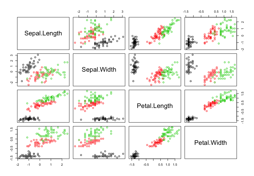
Figure 1: Pairs plot of the iris dataset.

Table 1: Gaussian mixture and KDE misclassification maps for the iris dataset.

Gaussian Mixture Map: $\left(\begin{tabular}[]{rrr}1.00&0.00&0.00\\ 0.00&0.98&0.02\\ 0.00&0.03&0.97\\ \end{tabular}\right)$

KDE Map: $\left(\begin{tabular}[]{rrr}1.00&0.00&0.00\\ 0.03&0.77&0.21\\ 0.00&0.17&0.83\\ \end{tabular}\right)$

It is interesting to note that when using KDE, there is more overlap than when using a Gaussian mixture. Perhaps, it can be explained by the fact that when using a mixture of Gaussian distributions for each component, naturally more points will be simulated closer to the centre of each component in the mixture. In the case of KDE estimation, the points in the tail of the distribution, more importantly the points which lie on the border of the two clusters, have the same probability of being chosen as the points in the centre.

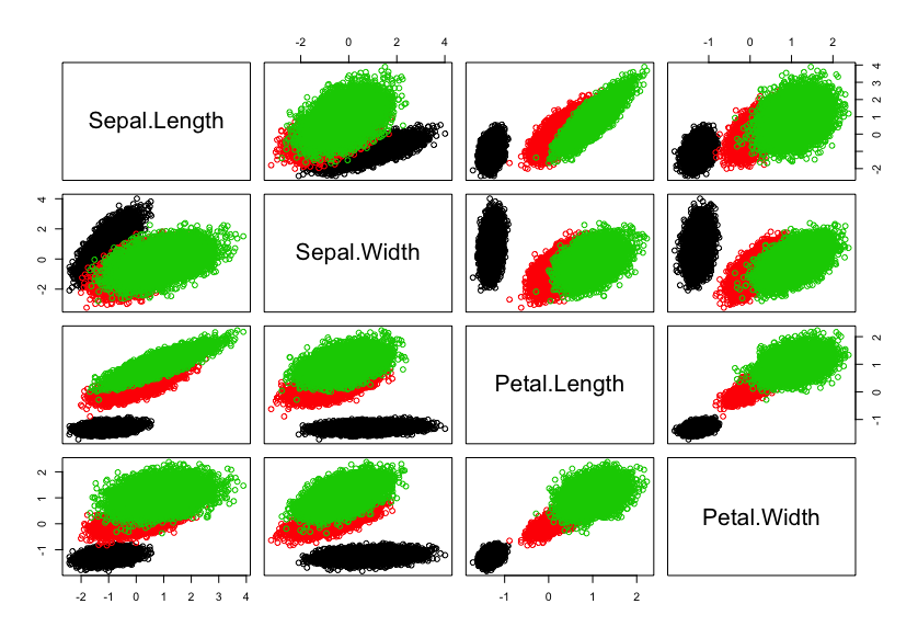
(a)

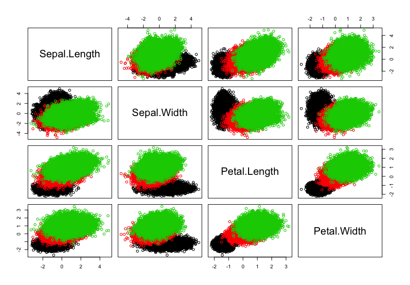
(b)

Figure 2: 1000 simulated points for each component of the iris dataset simulated using (a) a fitted mixture of Gaussian distributions and (b) using KDE.

3.2.2 General Applicability

It is important to note that in the scenario of a true cluster analysis this method for measuring cluster overlap is not applicable because the true group labels are not known. However, this is useful for the purposes presented here as we wish to determine if cluster separation does result in different performance for the two different methods. Moreover, this overlap procedure would be useful in other scenarios. One example would be in the case of a discriminant analysis, where the true labels are known. Another would be in the case determining separation of classes of categorical variables such as gender or race in regardless of the method of analysis.

3.3 Initialization and Convergence

In order to increase the chances of obtaining the maximum likelihood, many different starting values are considered and then the algorithm is ran to full convergence. Specifically, up to eleven k-means initializations, 1000 soft partitions, up to 100$G$ (where $G$ is the number of groups) unique hard initializations by running 1 iteration of the k-means algorithm, see Melnykov & Melnykov (2012) for details, and a hierarchical partition using Ward’s linkage (Ward 1963). Note that only 100$G$ hard initializations are considered because the number of unique hard partitions increases with $G$. In addition, although not applicable in practice, but useful for comparison purposes, initializing with the true labels is considered. The final results are obtained by taking the largest likelihood over all these initializations, with the exception of the true labels.

The same convergence criterion was used for both methods. Specifically, the EM algorithm is terminated when $(\ell^{(t+1)}-\ell^{(t)})/|\ell^{(t+1)}|<0.0001$, where $\ell^{(t)}$ is the estimated log-likelihood at iteration $t$.

4 Comparison Using Multiple Datasets

Using the initialization, model selection and convergence criteria outlined previously, we perform a comparison based on multiple real benchmarking datasets.

The first dataset we consider is the iris dataset described previously. Again, this dataset considers 150 observations from three different species of iris, on four variables. The results are summarized in Table 2 along with the skewness, kurtosis with their respective test p-values, and the classification maps. Both the skewness and kurtosis are not significantly different from what would be expected under multivariate normality. Moreover, as discussed previously, and as is well known with this dataset, the first species is well separated from species 2 and 3, and species 2 and three have a fair amount of overlap. The overall performance over these methods is identical in terms of the number of groups chosen, and the classification performance. The likelihood values are very comparable over all methods, and the lowest BIC is obtained by the power transformation; however, given the comparable likelihood values and the additional parameters, this difference is not really substantial.

Table 2: Results of the skewed models and transformation methods for the Iris dataset.

	Skewed Models			Transformations
	VG	GH		Manly	Power
Log-Likelihood	$-307.31$	$-311.04$		$-308.24$	$-306.81$
BIC	810.03	827.51		801.86	799.01
$\mathcal{M}$	39	41		37	37
$\hat{G}$	2	2		2	2
ARI	0.568	0.568		0.568	0.568
Confusion	$\left(\begin{tabular}[]{rrr}50&0\\ 0&50\\ 0&50\\ \end{tabular}\right)$	$\left(\begin{tabular}[]{rrr}50&0\\ 0&50\\ 0&50\\ \end{tabular}\right)$		$\left(\begin{tabular}[]{rrr}50&0\\ 0&50\\ 0&50\\ \end{tabular}\right)$	$\left(\begin{tabular}[]{rrr}50&0\\ 0&50\\ 0&50\\ \end{tabular}\right)$
$G=3$  $p=4$  $n:50+50+50=150$
Skewness: (2.90(0.24), 2.84(0.26), 2.97(0.21))
Kurtosis: (1.49(0.45), $-$2.03(0.30), $-$0.66(0.74))
KDE Map: $\left(\begin{tabular}[]{rrr}1.00&0.00&0.00\\ 0.03&0.77&0.21\\ 0.00&0.17&0.83\\ \end{tabular}\right)$  Gaussian Map: $\left(\begin{tabular}[]{rrr}1.00&0.00&0.00\\ 0.00&0.98&0.02\\ 0.00&0.03&0.97\\ \end{tabular}\right)$

The second dataset considered was the 13 variable wine dataset from the R package rattle (Williams 2011) which measures 13 chemical properties of 3 three different types of wine. Results are shown in Table 3. All four methods under fitted the true number of groups. This could be due to one of two reasons. The first is the dimensionality of the data and the fact that we are fitting an unconstrained covariance/scale matrix. However, this could also be due to the significant negative kurtosis for groups 1 and 3. Again, however, there is very little difference in the likelihood and BIC values. Moreover, in terms of classification performance, the results are very similar across methods.

Table 3: Results of the skewed models and transformation methods for the Wine dataset.

	Skewed Models			Transformations
	VG	GH		Manly	Power
Log-Likelihood	$-2188.94$	$-2189.30$		$-2153.58$	$-2144.87$
BIC	5605.96	5617.04		5524.88	5507.45
$\mathcal{M}$	237	239		235	235
$\hat{G}$	2	2		2	2
ARI	0.461	0.461		0.454	0.469
Confusion	$\left(\begin{tabular}[]{rrr}59&0\\ 66&5\\ 0&48\\ \end{tabular}\right)$	$\left(\begin{tabular}[]{rrr}59&0\\ 66&5\\ 0&48\\ \end{tabular}\right)$		$\left(\begin{tabular}[]{rrr}59&0\\ 65&6\\ 0&48\\ \end{tabular}\right)$	$\left(\begin{tabular}[]{rrr}59&0\\ 67&4\\ 0&48\\ \end{tabular}\right)$
$G=3$  $p=13$  $n:59+71+48=178$
Skewness: (47.27(0.37), 57.68(2.35e-11), 50.44(0.96))
Kurtosis: ($-13.62(8.05\text{e}-3)$, $10.22(0.029)$, $-16.63(3.52\text{e}-3)$)
KDE Map: $\left(\begin{tabular}[]{rrr}0.91&0.08&0.00\\ 0.06&0.90&0.04\\ 0.00&0.13&0.87\\ \end{tabular}\right)$  Gaussian Map: $\left(\begin{tabular}[]{rrr}1.00&0.00&0.00\\ 0.00&1.00&0.00\\ 0.00&0.00&1.00\\ \end{tabular}\right)$

The next dataset considered was the bankruptcy dataset from the R package MixGHD (Tortora et al. 2015) with the results shown in Table 4. For all four methods, the BIC chooses one component, and the BIC values are once again comparable. From the skewness and kurtosis measures and from looking at the plot of the data, it is clear that the first component (bankrupt firms) are non-Gaussian and the second group are approximately Gaussian. Moreover, the misclassification maps suggest overlap between these two clusters. This actually displays a general issue in the context of clustering. If a symmetric cluster overlaps with an asymmetric cluster and there is no information about the underlying group structure, then it will be very difficult to determine if there is one cluster or two. Moreover, as seen here, using skewed methods do not help in this scenario, as all four fail to capture the two group solution, and the Gaussian mixture over fits the number of groups. This is an area that should be addressed in future work, as it is quite possible using these methods can result in missing a possibly very important group.

Table 4: Results of the skewed models and transformation methods for the Bankruptcy dataset.

	Skewed Models			Transformations
	VG	GH		Manly	Power
Log-Likelihood	$-114.84$	$-110.85$		$-108.94$	$-106.54$
BIC	263.20	259.40		247.21	242.41
$\mathcal{M}$	8	9		7	7
$\hat{G}$	1	1		1	1
ARI	0.000	0.000		0.000	0.000
Confusion	$\left(\begin{tabular}[]{r}33\\ 33\\ \end{tabular}\right)$	$\left(\begin{tabular}[]{rr}33\\ 33\\ \end{tabular}\right)$		$\left(\begin{tabular}[]{rr}33\\ 33\\ \end{tabular}\right)$	$\left(\begin{tabular}[]{rr}33\\ 33\\ \end{tabular}\right)$
$G=2$  $p=2$  $n:33+33=66$
Skewness: $(15.33(<1\text{e}-16),0.54(0.56))$
Kurtosis: $(15.42(<1\text{e}-16),-1.43(0.30))$
KDE Map: $\left(\begin{tabular}[]{rr}0.84&0.16\\ 0.12&0.88\\ \end{tabular}\right)$  Gaussian Map: $\left(\begin{tabular}[]{rrr}0.98&0.02\\ 0.02&0.98\\ \end{tabular}\right)$

The diabetes dataset (Fraley et al. 2012) considers three measurements on 145 non-obese diabetes patients, with three types of diabetes which were classified as normal, overt and chemical, with results shown in Table 5. Again, very little difference is seen in the performance of the methods.

Table 5: Results of the skewed models and transformation methods for the Diabetes dataset.

	Skewed Models			Transformations
	VG	GH		Manly	Power
Log-Likelihood	$-178.75$	$-176.62$		$-171.68$	$-168.24$
BIC	491.88	497.57		467.77	480.80
$\mathcal{M}$	27	29		25	25
$\hat{G}$	2	2		2	2
ARI	0.465	0.450		0.465	0.488
Confusion	$\left(\begin{tabular}[]{rr}32&4\\ 76&0\\ 2&31\\ \end{tabular}\right)$	$\left(\begin{tabular}[]{rr}32&4\\ 75&1\\ 2&31\\ \end{tabular}\right)$		$\left(\begin{tabular}[]{rr}32&4\\ 76&0\\ 2&31\\ \end{tabular}\right)$	$\left(\begin{tabular}[]{rr}32&4\\ 76&0\\ 1&32\\ \end{tabular}\right)$
$G=3$  $p=3$  $n:36+76+33=145$
Skewness: $(9.74(7.09\text{e}-9),3.45(3.68\text{e}-6),7.22(1.92\text{e}-5))$
Kurtosis: $(8.73(1.72\text{e}-06),3.22(0.010),3.28(0.085))$
KDE Map: $\left(\begin{tabular}[]{rrr}0.47&0.40&0.13\\ 0.13&0.87&0.01\\ 0.09&0.25&0.66\\ \end{tabular}\right)$  Gaussian Map: $\left(\begin{tabular}[]{rrr}0.91&0.08&0.01\\ 0.02&0.98&0.00\\ 0.02&0.00&0.98\\ \end{tabular}\right)$

We also considered the AIS dataset (Azzalini 2018) which involves 11 measures from 100 female and 102 male athletes. Here we present the results for the three commonly used variables for this dataset, namely the BMI, body fat and lean body mass with the results in Table 6. Again, very little difference was seen in performance for the generalized hyperbolic and both transformation methods. What is interesting, however, is where these misclassifications lie. Specifically, the variance-gamma misclassifies more men than women whereas the generalized hyperbolic misclassifies more women than men. Moreover, when comparing the transformation methods, equal numbers of men and women are misclassified.

Table 6: Results of the skewed models and transformation methods for the AIS dataset.

	Skewed Models			Transformations
	VG	GH		Manly	Power
Log-Likelihood	$-619.22$	$-618.18$		$-620.77$	$-604.21$
BIC	1381.76	1390.29		1341.12	1347.50
$\mathcal{M}$	27	29		25	25
$\hat{G}$	2	2		2	2
ARI	0.847	0.922		0.922	0.922
Confusion	$\left(\begin{tabular}[]{rr}99&1\\ 7&95\\ \end{tabular}\right)$	$\left(\begin{tabular}[]{rr}97&3\\ 1&101\\ \end{tabular}\right)$		$\left(\begin{tabular}[]{rr}98&2\\ 2&100\\ \end{tabular}\right)$	$\left(\begin{tabular}[]{rr}98&2\\ 2&100\\ \end{tabular}\right)$
$G=2$  $p=3$  $n:100+102=202$
Skewness: $(2.54(6.53\text{e}-6),5.66(3.33\text{e}-16))$
Kurtosis: $(1.69(0.12),7.97(2.00\text{e}-13))$
KDE Map: $\left(\begin{tabular}[]{rr}0.89&0.11\\ 0.09&0.91\\ \end{tabular}\right)$  Gaussian Map: $\left(\begin{tabular}[]{rrr}0.98&0.02\\ 0.02&0.98\\ \end{tabular}\right)$

The last dataset considered herein was the famous crabs dataset, Venables & Ripley (2002). This considers two species of crab (blue and orange) and males and females within each species. The first group are the blue males, the second the blue females, the third the orange males, and the fourth the orange females. The results are shown in Table 7. What is very interesting, but not entirely clear from the overlap, skewness, and kurtosis from the four groups is that the skewed distribution methods separate the species perfectly, whereas the transformation methods discriminate based on gender. As all methods were run to convergence on many different initialization values, and the initializations were the same for each method, it is unlikely that it is due to the initialization. However, Table 8 shows the skewness and kurtosis values and their respective p-values based on sex and species, and it appears that the transformation methods found one skewed component and a symmetric component, whereas the skewed distribution methods found two skewed components. This might suggest that the transformation methods might be slightly more likely to find symmetric components than the skewed distributions.

Table 7: Results of the skewed models and transformation methods for the Crabs dataset.

	Skewed Models		Transformations
	VG	GH	Manly	Power
Log-Likelihood	165.25	162.12	144.68	144.62
BIC	$-49.69$	$-32.83$	$-19.16$	$2.17$
$\mathcal{M}$	53	55	51	51
$\hat{G}$	2	2	2	2
ARI	0.496	0.496	0.374	0.374
Confusion	$\left(\begin{tabular}[]{rrr}50&0\\ 50&0\\ 0&50\\ 0&50\\ \end{tabular}\right)$	$\left(\begin{tabular}[]{rrr}50&0\\ 50&0\\ 0&50\\ 0&50\\ \end{tabular}\right)$	$\left(\begin{tabular}[]{rrr}47&3\\ 6&44\\ 50&0\\ 4&46\\ \end{tabular}\right)$	$\left(\begin{tabular}[]{rrr}47&3\\ 6&44\\ 50&0\\ 4&46\\ \end{tabular}\right)$
$G=4$  $p=5$  $n:50+50+50+50=200$
Skewness: $(4.71(0.28),5.01(0.20),2.82(0.93),5.10(0.18))$
Kurtosis: $(-1.26(0.60),-0.80(0.73),-3.17(0.18),-0.18(0.94))$
KDE Map: $\left(\begin{tabular}[]{rrrr}0.33&0.25&0.29&0.13\\ 0.20&0.38&0.20&0.22\\ 0.26&0.18&0.37&0.19\\ 0.15&0.31&0.22&0.32\\ \end{tabular}\right)$  Gaussian Map: $\left(\begin{tabular}[]{rrrr}0.95&0.05&0.00&0.00\\ 0.04&0.96&0.00&0.00\\ 0.00&0.00&0.99&0.01\\ 0.00&0.00&0.01&0.98\\ \end{tabular}\right)$

Table 8: Skewness and kurtosis for the crabs dataset based on sex and species separately.

	Skewness (p-value)	Kurtosis (p-value)
Males	$2.7(0.12)$	$-2.38(0.15)$
Females	$3.64(0.0046)$	$-0.47(0.78)$
Blue	$4.9(1.30\text{e}-5)$	$0.87(0.6)$
Orange	$4.01(9.50\text{e}-4)$	$0.37(0.83)$

5 Discussion

From the analyses performed on a variety of datasets and the extensive number and type of initializations performed, it appears that no one method consistently outperforms the others, and usually the performance is very similar if not identical. Moreover, it does not appear that skewness, kurtosis and cluster overlap completely determines the relative performance of these methods. This is not to say, however, that there are no differences between the two methods. As seen with the crabs, the skewed models discriminate based on species, and the transformation methods on sex. Although not shown herein, the skewed models also discriminate based on sex when using k-means initializations, but when run using the more flexible initialization methods, found the species structure. The transformation methods, on the other hand, always found the sex structure. In terms of actual properties of the methods, transformation methods are more parsimonious, controlling for the number of groups, due to the lack of a concentration (or index) parameter. Therefore, it may not be a question of when one method might be preferable to another, but rather why one method might be preferable to another in the context of the analysis in question.

References

- (1)
- Anderson (1935) Anderson, E. (1935), ‘The irises of the Gaspé Peninsula’, Bulletin of the American Iris Society 59, 2–5.
-
Azzalini (2018)
Azzalini, A. (2018), The R package
sn: The Skew-Normal and Related Distributions such as the Skew-
(version 1.5-3)., Università di Padova, Italia.
http://azzalini.stat.unipd.it/SN - Baum et al. (1970) Baum, L. E., Petrie, T., Soules, G. & Weiss, N. (1970), ‘A maximization technique occurring in the statistical analysis of probabilistic functions of Markov chains’, Annals of Mathematical Statistics 41, 164–171.
- Browne & McNicholas (2015) Browne, R. P. & McNicholas, P. D. (2015), ‘A mixture of generalized hyperbolic distributions’, Canadian Journal of Statistics 43(2), 176–198.
- Fraley et al. (2012) Fraley, C., Raftery, A. E., Murphy, T. B. & Scrucca, L. (2012), mclust version 4 for R: Normal mixture modeling for model-based clustering, classification, and density estimation, Technical Report 597, Department of Statistics, University of Washington, Seattle, WA.
- Franczak et al. (2014) Franczak, B. C., Browne, R. P. & McNicholas, P. D. (2014), ‘Mixtures of shifted asymmetric Laplace distributions’, IEEE Transactions on Pattern Analysis and Machine Intelligence 36(6), 1149–1157.
-
Härdle & Müller (1997)
Härdle, W. & Müller, M. (1997), Multivariate and semiparametric kernel regression,
SFB 373 discussion paper, Humboldt University of Berlin, Berlin.
http://hdl.handle.net/10419/66292 - Karlis & Santourian (2009) Karlis, D. & Santourian, A. (2009), ‘Model-based clustering with non-elliptically contoured distributions’, Statistics and Computing 19(1), 73–83.
- Lee & McLachlan (2014) Lee, S. & McLachlan, G. J. (2014), ‘Finite mixtures of multivariate skew t-distributions: some recent and new results’, Statistics and Computing 24, 181–202.
- Lin (2010) Lin, T.-I. (2010), ‘Robust mixture modeling using multivariate skew t distributions’, Statistics and Computing 20(3), 343–356.
- Maitra & Melnykov (2010) Maitra, R. & Melnykov, V. (2010), ‘Simulating data to study performance of finite mixture modeling and clustering algorithms’, Journal of Computational and Graphical Statistics 19(2), 354–376.
- Manly (1976) Manly, B. (1976), ‘Exponential data transformations’, Journal of the Royal Statistical Society: Series D (The Statistician) 25(1), 37–42.
- Mardia (1970) Mardia, K. V. (1970), ‘Measures of multivariate skewness and kurtosis with applications’, Biometrika 57(3), 519–530.
- McNicholas (2016a) McNicholas, P. D. (2016a), Mixture Model-Based Classification, Chapman & Hall/CRC Press, Boca Raton.
- McNicholas (2016b) McNicholas, P. D. (2016b), ‘Model-based clustering’, Journal of Classification 33(3), 331–373.
- McNicholas et al. (2017a) McNicholas, S. M., McNicholas, P. D. & Browne, R. P. (2017a), A mixture of variance-gamma factor analyzers, in S. E. Ahmed, ed., ‘Big and Complex Data Analysis: Methodologies and Applications’, Springer International Publishing, Cham, pp. 369–385.
- McNicholas et al. (2017b) McNicholas, S. M., McNicholas, P. D. & Browne, R. P. (2017b), A mixture of variance-gamma factor analyzers, in S. E. Ahmed, ed., ‘Big and Complex Data Analysis, Contributions to Statistics’, Springer International Publishing, Cham, pp. 369–385.
- Melnykov (2016) Melnykov, V. (2016), ‘Merging mixture components for clustering through pairwise overlap’, Journal of Computational and Graphical Statistics 25(1), 66–90.
- Melnykov & Melnykov (2012) Melnykov, V. & Melnykov, I. (2012), ‘Initializing the EM algorithm in gaussian mixture models with an unknown number of components’, Computational Statistics & Data Analysis 56(6), 1381–1395.
- Melnykov & Zhu (2018) Melnykov, V. & Zhu, X. (2018), ‘On model-based clustering of skewed matrix data’, Journal of Multivariate Analysis 167, 181–194.
- Melnykov & Zhu (2019) Melnykov, V. & Zhu, X. (2019), ‘Studying crime trends in the USA over the years 2000–2012’, Advances in Data Analysis and Classification 13(1), 325–341.
- Morris & McNicholas (2013) Morris, K. & McNicholas, P. D. (2013), ‘Dimension reduction for model-based clustering via mixtures of shifted asymmetric Laplace distributions’, Statistics and Probability Letters 83(9), 2088–2093.
- Murray, Browne & McNicholas (2014) Murray, P. M., Browne, R. B. & McNicholas, P. D. (2014), ‘Mixtures of skew-t factor analyzers’, Computational Statistics and Data Analysis 77, 326–335.
- Murray et al. (2017) Murray, P. M., Browne, R. B. & McNicholas, P. D. (2017), ‘Hidden truncation hyperbolic distributions, finite mixtures thereof, and their application for clustering’, Journal of Multivariate Analysis 161, 141–156.
- Murray, McNicholas & Browne (2014) Murray, P. M., McNicholas, P. D. & Browne, R. B. (2014), ‘A mixture of common skew- factor analyzers’, Stat 3(1), 68–82.
- Nitithumbundit & Chan (2015) Nitithumbundit, T. & Chan, J. S. K. (2015), ‘An ECM algorithm for skewed multivariate variance gamma distribution in normal mean-variance representation’. arXiv preprint arXiv:1504.01239.
- O’Hagan et al. (2016) O’Hagan, A., Murphy, T. B., Gormley, I. C., McNicholas, P. D. & Karlis, D. (2016), ‘Clustering with the multivariate normal inverse Gaussian distribution’, Computational Statistics and Data Analysis 93, 18–30.
-
Revelle (2018)
Revelle, W. (2018), psych: Procedures
for Psychological, Psychometric, and Personality Research, Northwestern
University, Evanston, Illinois.
R package version 1.8.12.
https://CRAN.R-project.org/package=psych - Scott & Symons (1971) Scott, A. J. & Symons, M. J. (1971), ‘Clustering methods based on likelihood ratio criteria’, Biometrics 27, 387–397.
- Tang et al. (2018) Tang, Y., Browne, R. P. & McNicholas, P. D. (2018), ‘Flexible clustering of high-dimensional data via mixtures of joint generalized hyperbolic distributions’, Stat 7(1), e177.
- Tiedeman (1955) Tiedeman, D. V. (1955), On the study of types, in S. B. Sells, ed., ‘Symposium on Pattern Analysis’, Air University, U.S.A.F. School of Aviation Medicine, Randolph Field, Texas.
- Tortora et al. (2015) Tortora, C., Browne, R. P., Franczak, B. C. & McNicholas, P. D. (2015), MixGHD: Model Based Clustering, Classification and Discriminant Analysis Using the Mixture of Generalized Hyperbolic Distributions. R package version 1.8.
- Tortora et al. (2019) Tortora, C., Franczak, B. C., Browne, R. P. & McNicholas, P. D. (2019), ‘A mixture of coalesced generalized hyperbolic distributions’, Journal of Classification 36(1), 26–57.
- Venables & Ripley (2002) Venables, W. N. & Ripley, B. D. (2002), Modern Applied Statistics with S, fourth edn, Springer, New York.
- Vrbik & McNicholas (2012) Vrbik, I. & McNicholas, P. D. (2012), ‘Analytic calculations for the EM algorithm for multivariate skew-t mixture models’, Statistics and Probability Letters 82(6), 1169–1174.
- Vrbik & McNicholas (2014) Vrbik, I. & McNicholas, P. D. (2014), ‘Parsimonious skew mixture models for model-based clustering and classification’, Computational Statistics and Data Analysis 71, 196–210.
- Ward (1963) Ward, J. H. (1963), ‘Hierarchical grouping to optimize an objective function’, Journal of the American Statistical Association 58, 236–244.
- Williams (2011) Williams, G. (2011), Data mining with Rattle and R: The art of excavating data for knowledge discovery, Springer Science & Business Media.
- Wolfe (1965) Wolfe, J. H. (1965), A computer program for the maximum likelihood analysis of types, Technical Bulletin 65-15, U.S. Naval Personnel Research Activity.
- Yeo & Johnson (2000) Yeo, I.-K. & Johnson, R. A. (2000), ‘A new family of power transformations to improve normality or symmetry’, Biometrika 87(4), 954–959.
- Zhu & Melnykov (2018) Zhu, X. & Melnykov, V. (2018), ‘Manly transformation in finite mixture modeling’, Computational Statistics & Data Analysis 121, 190–208.