Tempered stable distributions
and finite variation
Ornstein-Uhlenbeck processes

Abstract

Constructing Lévy-driven Ornstein-Uhlenbeck processes is a task closely related to the notion of self-decomposability. In particular, their transition laws are linked to the properties of what will be hereafter called the $a$-remainder of their self-decomposable stationary laws. In the present study we fully characterize the Lévy triplet of these $a$-remainders and we provide a general framework to deduce the transition laws of the finite variation Ornstein-Uhlenbeck processes associated with tempered stable distributions. We focus finally on the subclass of the exponentially-modulated tempered stable laws and we derive the algorithms for an exact generation of the skeleton of Ornstein-Uhlenbeck processes related to such distributions, with the further advantage of adopting a procedure computationally more efficient than those already available in the existing literature.

Keywords: Lévy-driven Ornstein-Uhlenbeck Processes; Self-decomposable Laws; Tempered Stable Distributions; Simulations

1 Introduction

The Lévy-driven Ornstein-Uhlenbeck (OU) processes have attracted considerable interest in recent studies because of their potential applications to a wide range of fields. As observed in Barndorff-Nielsen and Shephard [3], these OU process are mathematically tractable and can be seen as the continuous-time analogues of the autoregressive AR($1$) processes (see Wolfe [41]). They constitute indeed a rich and flexible class that can accommodate features such as jumps, semi-heavy tails and asymmetry which are well evident in the real physical phenomena as well as in the financial data. The energy and commodity markets exhibit for instance a strong mean-reversion and sudden spikes which makes the use of the Lévy-driven OU-processes more advisable than the standard Gaussian framework. In addition, several approaches based on Lévy processes such as the Variance Gamma (VG) or the Normal Inverse Gaussian (NIG) have been proposed to overcome the known limits of the usual Black-Scholes model (see Madan and Seneta [29] and Barndorff-Nielsen [2]): all these non Gaussian noises can of course be adopted as the drivers of OU processes. Example of their applications to mathematical finance can be found in Benth and Pircalabu [6] and Cufaro Petroni and Sabino [12] in the context of energy markets, in Bianchi and Fabozzi [8] for the modeling of credit risk and in Barndorff-Nielsen and Shephard [3] for stochastic volatility modeling.

The distributional properties of a non-Gaussian process of OU-type are closely related to the notion of self-decomposability (sd), because as noted in Barndorff-Nielsen and Shephard [3] and in Taufer and Leonenko [40], the stationary law of such a process must be sd. We recall here that a law with chf $\eta(u)$ is said to be sd (see Sato [38], Cufaro Petroni [11]) when for every $0<a<1$ we can find another law with chf $\chi_{a}(u)$ such that

$$\eta(u)=\eta(au)\chi_{a}(u).$$ (1)

Of course a random variable (rv) $X$ with chf $\eta(u)$ is also said to be sd when its law is sd, and looking at the definitions this means that for every $0<a<1$ we can always find two independent rv’s – a $Y$ with the same law of $X$, and a $Z_{a}$ with chf $\chi_{a}(u)$ – such that in distribution

$$X\stackrel{{\scriptstyle d}}{{=}}aY+Z_{a}$$ (2)

Hereafter the rv $Z_{a}$ will be called the $a$-remainder of $X$ and in general has an infinitely divisible distribution (id) (see Sato [38]). We will show in the following (see also Barndorff-Nielsen [2], Sabino and Cufaro Petroni [37] and Sabino [35]) that the transition law between the times $t$ and $t+\Delta t$ of a Lévy-driven OU process $X(t)$ essentially coincides indeed with the law of the $a$-remainder of its sd-stationary distribution, provided that $a=e^{-b\Delta t}$ where $b$ is the OU mean-reversion rate. It is therefore natural to investigate the properties of the $a$-remainder of a certain sd law even irrespective of its possible relation to the theory of the OU processes.

The first step in this inquiry apparently is the characterization of the Lévy triplet of the $a$-remainder of a sd law: this would of course constitute a crucial building block in the construction of a Lévy-driven OU processes. We will thereafter focus our attention on the class of the tempered stable (TS) distributions (see for instance see Rosiński [34] and Grabchak [17]) with finite variation, and we will provide a general framework to derive their transition laws from their associated $a$-remainders. There are in fact two standard ways to associate a TS distribution to an OU process $X(\cdot)$: if its stationary law is a TS distribution we will say that $X(\cdot)$ is a TS-OU process; if on the other hand, $X(\cdot)$ is driven by a TS background noise we will say that $X(t)$ is a OU-TS process.

Some of the results discussed in the following sections are not new: Kawai and Masuda [23, 24] and Zhang [42], for instance, have considered OU processes whose stationary marginal law is an exponentially-modulated TS distribution hereafter called a classical TS (CTS), whereas Bianchi et al. [7] have taken into account the rapidly decreasing TS laws (RDTS), and Grabchak [20] finally merged all these laws in the larger class of the general TS distributions. Recently Qu et al [33] have also studied both CTS-OU and OU-CTS processes. In this perspective a first contribution of the present paper consists in harmonizing these results in the scheme of the $a$-remainders, and in showing the further advantages of this approach: some of the theorems in the aforementioned literature become indeed special cases of this proposed comprehensive framework. On the other hand – by exploiting properties valid for every id distribution – an explicit knowledge of the Lévy triplet of the $a$-remainder makes very easy and straightforward the calculation of the cumulants of the transition law of a OU process. This turns out in particular to be a remarkable asset in testing the efficiency of the simulation algorithms and can be adopted for the parameters estimation. It is also worthwhile remarking that the laws of the $a$-remainders are in fact id, and therefore they lend the possibility of producing an entire new class of associated Lévy processes as shown for instance in Gardini et al. [16, 15].

Finally, as done in Qu et al [33], we focus our attention on the case of the CTS related OU processes with their transition laws, both for the OU-CTS and the CTS-OU cases, but within the perspective of the $a$-remainders. We also derive a few new algorithms intended to simulate the skeleton of such processes. We find in particular that for the simulation of the CTS-OU processes our procedure is computationally more efficient than that of Zhang [42] because it does not rely on an acceptance rejection method (other than that required to draw from a CTS law), but rather on the inverse method (see Devroye [13]). We adopted instead a procedure based on an acceptance rejection method for the OU-CTS process that however, at variance with that of Qu et al [33], has the advantage of having an expected number of iterations before acceptance that can always be kept arbitrarily close to $1$.

The paper is organized as follows: the Section 2 introduces the notations and the preliminary notions. In particular it presents the basic properties of non-Gaussian OU processes and their relation with the sd laws. In the Section 3 we then derive the Lévy triplet of the $a$-remainder of an arbitrary sd law, and in particular that of the $a$-remainder of a general TS distribution with finite variation. These results are instrumental to explicitly write down the transition law of CTS-OU process. In the subsequent Section 5 we focus on the OU-CTS processes, and in Section 6 we present the algorithms for the simulation of the skeleton of both the CTS-OU and the OU-CTS processes pointing out their differences and their advantages with respect to the solutions already existing in the literature. The Section 7 illustrates the effectiveness of our simulation schemes by comparing the true values and the Monte Carlo estimated values of the first four cumulants. We also consider some approximation schemes to further check the performance of our procedures and we propose a simple approach to the parameters calibration. Finally the Section 8 concludes the paper with an overview of future inquiries and of possible further applications.

2 Notations and preliminary remarks

Take a – possibly non-Gaussian – one-dimensional Lévy process $L(\cdot)$, and the Ornstein-Uhlenbeck () process $X(\cdot)$ solution of the stochastic differential equation (SDE)

$$dX(t)=-bX(t)dt+dL(t)\quad\qquad X(0)=X_{0}\quad\bm{P}\hbox{-\emph{a.s.}}\qquad b>0$$ (3)

to wit

$$X(t)=X_{0}\,e^{-bt}+Z(t)\qquad\quad Z(t)=\int_{0}^{t}e^{-b\,(t-s)}dL(s)$$ (4)

Hereafter $L(\cdot)$ will be called background driving Lévy process (BDLP) and $L(t)$ will also represent its stationary increment of width $t$ that completely define the process, but for an arbitrary initial condition. It is known that the chf (characteristic function) $\varphi_{L}(u,t)$ of these increments, and their lch (logarithmic characteristic) $\psi_{L}(u,t)=\ln\varphi_{L}(u,t)$ are retrievable from a given id (infinitely divisible) law with chf $\varphi_{L}(u)=e^{\psi_{L}(u)}$ according to

$$\varphi_{L}(u,t)=\varphi_{L}(u)^{t/T}\qquad\qquad\psi_{L}(u,t)=\frac{t}{T}\psi_{L}(u)$$

Here $T$ represents an arbitrary constant time scale introduced to keep a fair balance among the physical dimensions: for practical purposes however it is possible to take $T=1$, as we will do later on in the present paper. Note that here the given id $\varphi_{L}(u)$ and $\psi_{L}(u)$ can also be considered as shorthand notations for $\varphi_{L}(u,T)$ and $\psi_{L}(u,T)$, namely the characteristics of the rv (random variable) $L(T)$ famously eponym of our BDLP.

Following a Barndorff-Nielsen and Shephard [3] convention, if $\overline{\mathcal{D}}$ is the law of the stationary process we will say that $X(\cdot)$ is a $\overline{\mathcal{D}}$-OU process; when on the other hand the rv $L(T)$ is distributed according to the id law ${\mathcal{D}}$ we will say that $X(\cdot)$ is an OU-${\mathcal{D}}$ process. A well-known result (see for instance Cont and Tankov [10] or Sato [38]) states that a distribution $\overline{\mathcal{D}}$ can be the stationary law of a given OU-${\mathcal{D}}$ process if and only if $\overline{\mathcal{D}}$ is self-decomposable (sd, see more below). In addition, just by taking an arbitrary degenerate initial condition $X_{0}=x_{0},\;\bm{P}\hbox{-\emph{a.s.}}$ – and if we can manage to retrieve the distribution of its second, integral term $Z(t)$ – from the pathwise solution (4) it is also apparently possible to deduce the transition pdf (probability density function) of the Markov process $X(\cdot)$, and therefore all its distributional details in an explicit form. It is appropriate to point out moreover that in the equation (4) we provided the solution in terms of the original BDLP $L(t)$ rather than of the dimensionless time BDLP $L(b\,t)$ as done in Barndorff-Nielsen and Shephard [3]: therefore a few results of ours will turn out to be explicitly dependent on the parameter $b$. The differences between these two equivalent representations are also discussed in Barndorff-Nielsen [2], Barndorff-Nielsen and Shephard [4] or Schoutens [39] page 48.

Going back now to the SDE (3) it is possible to see (see also Barndorff-Nielsen et al. [1]) that the solution process (4) is stationary if and only if its chf $\varphi_{X}(u,t)$ is constant in time and steadily coincides with the chf $\overline{\varphi}_{X}(u)$ of the (sd) invariant initial distribution that turns out to be decomposable according to

$$\overline{\varphi}_{X}(u)=\overline{\varphi}_{X}(u\,e^{-b\,t})\varphi_{Z}(u,t)$$

where now, at every given $t$, $\varphi_{Z}(u,t)=e^{\psi_{Z}(u,t)}$ denotes the id chf of the rv $Z(t)$ in (4). This last statement apparently means that the law of $Z(t)$ in the solution (4) coincides with that of the $a$-remainder of the sd, stationary law $\overline{\varphi}_{X}$ provided that $a=e^{-b\,t}$, and that moreover we have

$$\varphi_{Z}(u,t) = \frac{\overline{\varphi}_{X}(u)}{\overline{\varphi}_{X}(u\,e^{-b\,t})}$$ (5)

$$\psi_{Z}(u,t) = \overline{\psi}_{X}(u)-\overline{\psi}_{X}(u\,e^{-b\,t}).$$ (6)

It turns out therefore that studying the transition law of an OU process essentially amounts to find first its stationary law, and then the law of its $a$-remainder (5): it is easy indeed to see from (4) that the chf of the time homogeneous transition law with a degenerate initial condition $X(0)=x_{0},\;\bm{P}\hbox{-\emph{a.s.}}$ is

$$\varphi_{X}(u,t|x_{0})=e^{\,ix_{0}ue^{-bt}}\varphi_{Z}(u,t)=\frac{\overline{\varphi}_{X}(u)\,e^{\,ix_{0}ue^{-bt}}}{\overline{\varphi}_{X}(u\,e^{-b\,t})}$$ (7)

As a consequence one can focus on the properties of the $a$-remainders of these sd distributions in order to deduce also the transition pdf of the associated OU processes. On the other hand, since the law of an $a$-remainder also is id, one could even construct its associated Lévy process resulting in an even wider range of possible models (see for instance Gardini et al. [15, 16]).

A number of additional relations between the distribution of the stationary process, and that of the rv $L(T)$ are known: it is possible to show for instance that between the lch’s $\overline{\psi}_{X}(u)=\ln\overline{\varphi}_{X}(u)$ of the stationary distribution, and $\psi_{L}(u)=\ln\varphi_{L}(u)$ of $L(T)$ the following relation holds (see Taufer and Leonenko [40] and Schoutens [39])

$$\overline{\psi}_{X}(u)=\frac{1}{T}\int_{0}^{+\infty}\psi_{L}(u\,e^{-bs})ds$$ (8)

On the other hand, assuming for simplicity that the Lévy measure of $L(T)$ and that of the stationary process admit densities – respectively denoted as $\nu_{L}(x)$ and $\overline{\nu}_{X}(x)$ – and supposing that $\overline{\nu}_{X}(x)$ is differentiable, it also results (see Sato [38], Cont and Tankov [10])

$$\overline{\nu}_{X}(x)=\frac{U(x)}{Tb\,|x|}\qquad\qquad U(x)=\left\{\begin{array}[]{ll}\int_{-\infty}^{x}\nu_{L}(y)dy&x<0\\ \int_{x}^{+\infty}\nu_{L}(y)dy&x>0\end{array}\right.$$ (11)

$$\overline{\nu}_{X}(x)+x\overline{\nu}_{X}^{\prime}(x)=-\frac{\nu_{L}(x)}{Tb}\qquad\qquad x\neq 0$$ (12)

Taking advantage finally of (6), (7) and (8) it is easy to see that the transition lch of the OU process can also be written in terms of the corresponding $\psi_{L}(u)$ of $L(T)$ in the form

$$\psi_{X}(u,t|x_{0})=iux_{0}e^{-bt}+\psi_{Z}(u,t)=iux_{0}e^{-b\,t}+\int_{0}^{t}\psi_{L}\left(ue^{-b\,s}\right)ds.$$ (13)

As a consequence we can also calculate the cumulants $c_{X,k}(x_{0},t),\;k=1,2,\ldots$ of $X(t)$ for $X_{0}=x_{0}$ from the cumulants $c_{L,k}$ of $L(T)$ according to

$$c_{X,1}(x_{0},t) = \bm{E}\left[{X(t)|X_{0}=x_{0}}\right]\;=\;x_{0}e^{-b\,t}+\frac{c_{L,1}}{b\,T}\left(1-e^{-b\,t}\right),\qquad k=1$$ (14)

$$c_{X,k}(x_{0},t) = \frac{c_{L,k}}{k\,b\,T}\left(1-e^{-k\,b\,t}\right),\qquad\qquad\qquad\qquad\qquad\qquad k=2,3,\ldots$$ (15)

On the other hand according to (6) the said cumulants $c_{X,k}(x_{0},t),\;k=1,2,\ldots$ for $X_{0}=x_{0}$ can also be derived from those of the stationary law here denoted $c_{\overline{X},k}$

$$c_{X,1}(x_{0},t) = \bm{E}\left[{X(t)|X_{0}=x_{0}}\right]\;=\;x_{0}e^{-b\,t}+c_{\overline{X},1}\left(1-e^{-b\,t}\right),\qquad k=1$$ (16)

$$c_{X,k}(x_{0},t) = c_{\overline{X},k}\left(1-e^{-k\,b\,t}\right),\qquad\qquad\qquad\qquad\qquad k=2,3,\ldots$$ (17)

These quantities can be used both as benchmarks to test the performance of the simulation algorithms, and to carry out an estimation procedure based on the generalized method of moments.

By summarizing (see also Sabino [35]), determining the transition law of the OU processes $X(\cdot)$ consists of two steps, that of course can also be used to produce a simulation algorithm:

• given the BDLP $L(\cdot)$, find the the stationary distribution $\overline{\varphi}_{X}(u)$ of (3);

• from (5) find the distribution of its $a$-remainder $Z(\cdot)$ with $a=e^{-b\,t}$.

In particular, the sequential generation of the process skeleton on a time grid $t_{0},t_{1},\dots,t_{M}$ will consist now in finding a simulation algorithm for the $a$-remainder $Z(\cdot)$ of the stationary law: assuming indeed at each step $a_{i}=e^{-b(t_{i}-t_{i-1})},\;i=0,\dots,M$, we just implement the following recursive procedure with initial condition $X(t_{0})=x_{0}$:

$$X(t_{i})=a_{i}X(t_{i-1})+Z_{a_{i}},\quad\qquad i=1,\dots,M.$$ (18)

where from (5) $Z_{a_{i}}$ are rv’s with chf’s

$$\chi_{i}(u,t)=\frac{\overline{\varphi}_{X}(u)}{\overline{\varphi}_{X}(u\,e^{-b(t_{i}-t_{i-1})})}$$

The previous equations suggest in some way two procedures to derive the properties of the transition law of an OU process: the first makes a start from its stationary law, the second from the law of its BDLP. In the following sections we will explore both directions focusing our attention on the tempered stable laws (TS; see Rosiński [34]) with finite variation (for details see Cont and Tankov [10]), and we will analyze both the TS-OU and the OU-TS processes. To this end, we recall that the finite variation TS laws have Lévy densities of the form

$$\nu(x)=c\,\frac{q(x)}{|x|^{1+\alpha}}\qquad\quad c>0,\quad 0\leq\alpha<1$$ (19)

where the tempering term $q(x)$ with $q(0)=1$ is monotonically decreasing and $q(+\infty)=0$ for $x>0$, and monotonically increasing and $q(-\infty)=0$ for $x<0$. We do not adopt however the full characterization of Rosiński [34] because we will focus on one-dimensional laws only, and mainly on the exponentially modulated TS, also known as classical tempered stable laws (CTS), where $q(x)=e^{-\beta_{1}x}$ for $x\geq 0$, while $q(x)=e^{\beta_{2}x}$ for $x<0$ with $\beta_{1},\beta_{2}>0$.

3 The TS distributions and their $a$-remainders

In the forthcoming sections we will discuss both the TS-OU and the OU-TS processes looking in particular to the properties of the $a$-remainder of their stationary laws, and we will focus our attention chiefly on the CTS subfamily. It is worthwhile noticing first that the study of these processes has extensively been carried on in the literature and that several types of TS laws have been investigated. For instance, Kawai and Masuda [23, 24] and Zhang [42] have considered OU processes whose stationary marginal law is a CTS distribution, whereas Bianchi et al. [7] assume a rapidly decreasing TS law (RDTS) and Grabchak [20] finally harmonizes all these types of laws considering the larger class of general TS distributions. Albeit many results can consequently be found in the literature cited so far, we will nevertheless elaborate a little on this topic also to show how the proofs of the propositions can be carried out in a simple way by taking advantage of the properties of the $a$-remainders and of their Lévy triplets. For this purpose let us remember in particular that, as it is well-known, the sd laws constitute a subclass of the class of the id distributions having an absolutely-continuous Lévy measure with density

$${\nu}(x)=\frac{k(x)}{|x|}$$

where $k(x)$ is increasing in $(-\infty,0)$ and decreasing in $(0,+\infty)$ (see Cont and Tankov [10], Proposition 15.3). Remark then that every TS distribution satisfying (19) also is sd. The law of the $a$-remainder of a sd law is id too (see Sato [38]) and the following proposition characterizes it in terms of its Lévy triplet.

Proposition 3.1.

Consider a sd law with Lévy triplet $(\gamma,\sigma,\nu)$, then for every $0<a<1$ the law of its $a$-remainder has Lévy triplet $(\gamma_{a},\sigma_{a},\nu_{a})$:

$$\gamma_{a} = \gamma(1-a)-a\int_{\mathbb{R}}\operatorname{sign}(x)(\mathds{1}_{|x|\leq\frac{1}{a}}-\mathds{1}_{|x|\leq 1})k(x)\,dx$$ (20)

$$\sigma_{a} = \sigma\sqrt{(1-a^{2})}$$ (21)

$$\nu_{a}(x) = \frac{k(x)-k(^{x}/_{a})}{|x|}\;=\;\nu(x)-\frac{\nu\left({}^{x}/_{a}\right)}{a}$$ (22)

Proof.

The Lévy-Khintchin representation of the lch of our sd law can be given in two equivalent ways just by redefining the drift term:

$$\psi(u) = \left\{\begin{array}[]{l}iu\gamma-\frac{1}{2}\sigma^{2}u^{2}+\int_{\mathbb{R}}\left(e^{iux}-1-iux\mathds{1}_{|x|\leq 1}\right)\frac{k(x)}{|x|}dx\\ iu\gamma^{\prime}-\frac{1}{2}\sigma^{2}u^{2}+\int_{\mathbb{R}}\left(e^{iux^{\prime}}-1-iux^{\prime}\mathds{1}_{|x^{\prime}|\leq\frac{1}{a}}\right)\frac{k(x^{\prime})}{|x^{\prime}|}dx^{\prime}\end{array}\right.$$ (25)

$$\gamma^{\prime} = \gamma+\int_{\mathbb{R}}\operatorname{sign}(x)(\mathds{1}_{|x|\leq\frac{1}{a}}-\mathds{1}_{|x|\leq 1})\,k(x)\,dx$$

Therefore, using both the representations (25) with the change of variable $x=ax^{\prime}$ in the second integral, the lch of the $a$-remainder $\psi_{a}(u)=\psi(u)-\psi(au)$ becomes

$$\psi_{a}(u) = iu\gamma(1-a)-a\,\int_{\mathbb{R}}\operatorname{sign}(x)(\mathds{1}_{|x|\leq\frac{1}{a}}-\mathds{1}_{|x|\leq 1})\,k(x)\,dx$$

$$\qquad\qquad-\frac{\sigma^{2}(1-a^{2})u^{2}}{2}+\int_{\mathbb{R}}\left(e^{iux}-1-iux\mathds{1}_{|x|\leq 1}\right)\frac{k(x)-k(^{x}/_{a})}{|x|}dx$$

Due to the properties of $k(x)$ it turns out that $k(x)-k(^{x}/_{a})>0$ for every $x$ and for every $0<a<1$; and, as it also happens that with $\nu_{a}(x)$ defined in (22) we have

$$\int_{\mathbb{R}}(1\wedge x^{2})\nu_{a}(x)dx<+\infty$$

it is easy to see that $\nu_{a}(x)$ qualify as a Lévy measure. Then $(\gamma_{a},\sigma_{a},\nu_{a})$ represents the legitimate Lévy triplet of the law of the $a$-remainder of a sd law. ∎

In the context of the OU processes where the law of $Z(t)$ in (4) at the time $t$ is the $a$-remainder of the stationary law for $a=e^{-bt}$, the Proposition 3.1 along with the equation (11) enables us to connect the Lévy density $\nu_{Z}(x,t)$ of the id rv $Z(t)$ at the time $t$ to $\overline{\nu}_{X}(x)$ and $\nu_{L}(x)$, the Lévy densities respectively of the sd stationary law and of the BDLP $L(T)$ at time $T$:

$$\nu_{Z}(x,t) = \frac{\overline{k}_{X}(x)-\overline{k}_{X}(^{x}/_{a})}{|x|}\;=\;\overline{\nu}_{X}(x)-\frac{\overline{\nu}_{X}(^{x}/_{a})}{a}\qquad\qquad\qquad a=e^{-b\,t}$$ (29)

$$= \frac{U(x)-U\left({}^{x}/_{a}\right)}{Tb\,|x|}\;=\;\frac{1}{Tb\,|x|}\left\{\begin{array}[]{ll}\int_{\,{}^{x}\!/_{a}}^{x}\nu_{L}(y)dy&\;\hbox{$x<0$}\\ \\ \int_{x}^{\,{}^{x}\!/_{a}}\nu_{L}(y)dy&\;\hbox{$x>0$}\end{array}\right.$$

According to the previous representations we can therefore adopt one of two possible strategies to study the properties of the transition law of a Lévy-driven OU process: the first based on the stationary law and more suitable for a $\overline{\mathcal{D}}$-OU process; the second using the distribution of the BDLP and more suitable for an OU-$\mathcal{D}$ process.

A Lévy process is said to be of finite variation when its trajectories are of finite variation with probability $1$, and it is possible to prove (Cont and Tankov [10]) that this happens if and only if its characteristic triplet $(\gamma,\sigma,\nu)$ satisfies the conditions

$$\sigma=0,\qquad\qquad\int_{|x|\leq 1}x\,\nu(x)\,dx<+\infty$$ (30)

An important subclass of such processes is that of subordinators that are Lévy processes with almost surely non-decreasing sample paths: in this event their Lévy triplet must satisfy the conditions

$$\sigma=0,\qquad\qquad\nu(x)=0\qquad x<0,\qquad\qquad\int_{0}^{+\infty}(x\wedge 1)\,\nu(x)\,dx<+\infty$$ (31)

As a matter of fact it would also be easy to see from the Lévy-Khintchin characterization theorem that any process of finite variation can be written as the difference of two independent subordinators – for instance the Variance Gamma (VG) processes can be represented as the difference of two Gamma processes – and therefore, without loss of generality, we can focus our attention on subordinators only. Without presuming now that the actual processes involved are of finite variation, subordinators or even Lévy processes, we will say hereafter for short that an id law with Lévy triplet $(\gamma,\sigma,\nu)$ is of finite variation when it satisfies the conditions (30), and is a subordinator when it satisfies the conditions (31). Finally we will assume for simplicity $\gamma=0$ because a non zero value would correspond just to a constant shift.

Proposition 3.2.

Consider a TS law with Lévy triplet $(0,0,\nu)$ such that $\nu(x)=0$ for $x<0$ and

$$\nu(x)=c\,\frac{q(x)}{x^{1+\alpha}}\quad\qquad x>0,\qquad c\geq 0,\qquad 0\leq\alpha<1$$ (32)

where $q(x)$ is a tempering function such that $q(x)-q(\gamma\,x)=o(x^{\alpha})$, $x\rightarrow 0^{+}$ for every $\gamma>0$. Then the Lévy density of its $a$-remainder is

$$\nu_{a}(x)=\nu_{1}(x)+\nu_{2}(x),\quad\left\{\begin{array}[]{l}\nu_{1}(x)=c\,(1-a^{\alpha})\frac{q(x)}{x^{1+\alpha}}\\ \\ \nu_{2}(x)=c\,a^{\alpha}\,\frac{q(x)\,-\,q(\,^{x}\!/_{a})}{x^{1+\alpha}}\end{array}\right.\quad\lambda_{a}=\!\!\int_{0}^{+\infty}\!\!\!\!\nu_{2}(x)dx<+\infty$$ (33)

Proof.

As already remarked every TS is sd and, if confined to $x>0$, it is easy to see that (31) is satisfied so that the law is a subordinator and hence also of finite variation. As a consequence there is an $a$-remainder and from Proposition 3.1 we have

$$\nu_{a}(x) = \nu(x)-\frac{\nu(\,^{x}/_{a})}{a}\;=\;(1-a^{\alpha})\nu(x)+a^{\alpha}\nu(x)-\frac{\nu(\,^{x}/_{a})}{a}$$

$$= c\,(1-a^{\alpha})\frac{q(x)}{x^{1+\alpha}}+ca^{\alpha}\frac{q(x)-q(\,^{x}/_{a})}{x^{1+\alpha}}\;=\;\nu_{1}(x)+\nu_{2}(x)$$

Now, while $\nu_{1}(x)$ is just a rescaled form of the original TS Lévy measure, we find that $\nu_{2}(x)>0$ is also normalizable. From the properties of $q(x)$ we have indeed that

$$\frac{q(x)-q(\,^{x}/_{a})}{x^{1+\alpha}}=o\,(x^{-1-\alpha}),\qquad\quad x\rightarrow+\infty,\qquad\quad 0<\alpha<1$$

while from our hypothesis we have

$$\frac{q(x)-q(\,^{x}/_{a})}{x^{1+\alpha}}=o(x^{-1}),\qquad\quad x\rightarrow 0^{+}.$$

and the integral in (33) turns out to be finite ∎

Under the conditions of the Proposition 3.2 we have found that $\nu_{2}(x)$ is an integrable non-negative function with $\Lambda_{a}$ in (33) playing the role of a normalization constant, and therefore that $g_{a}(x)=\nu_{2}(x)/\Lambda_{a}$ can be interpreted a full fledged pdf. As a consequence $\nu_{2}(x)$ can be considered as the Lévy measure density of a compound Poisson law of parameter $\Lambda_{a}$ and jump length distributed according to the pdf $g_{a}(x)$. Since on the other hand $\nu_{1}(x)$ is the Lévy measure density of the original TS law but with the rescaled parameter $c(1-a^{\alpha})$, according to the previous proposition we can claim that the $a$-remainder $Z_{a}$ of a TS law with Lévy density (32) is – in distribution – the sum $Y_{a}+C_{a}$ of two independent rv’s: a TS $Y_{a}$ of the type (32) with parameter $c(1-a^{\alpha})$, and a compound Poisson rv

$$C_{a}=\sum_{k=1}^{N_{a}}J_{a,k}$$

where $N_{s}$ is a Poisson rv of parameter $\Lambda_{a}$ and $J_{a,k},\;k=1,2,\ldots$ are a sequence of iid rv’s with pdf $g_{a}(x)$

As can be seen from (7) in the Section 2, the transition law of a generalized OU process (4) directly follows from the $a$-remainder of its sd stationary distribution when we take $a=e^{-b\,t}$. Adding in the results of the Proposition 3.2 we can therefore fully display the Lévy measure of the said transition laws when the stationary distribution is a TS subordinator with Lévy density (32). This class of laws is not without merits in itself and is a relevant one-dimensional subfamily of the general tempered stable laws discussed in Grabchak  [20]. It includes on the other hand the CTS subordinators with $0\leq\alpha<1$, while in fact the Theorem 1 in Zhang [43] for Inverse Gaussian-OU processes (IG-OU) and the Theorem 1 in Zhang [42] for TS-OU are special cases of the Proposition 3.2. The proposition also covers the $p\,$TS-OU introduced in Grabchak [17], the special case of Rapidly Decreasing TS-OU (RDTS-OU) discussed in Kim et al [26] and Bianchi et al. [7], the Modified TS-OU (MTS-OU) studied in Kim et al. [25], and the Bessel TS-OU (BTS-OU) discussed in Chung [9]. It is expedient to notice at this point that, although for a fixed time $t$ the law of $Z(t)$ defined in (4) is id and coincides with that of the $a$-remainder of the stationary law taking $a=e^{-b\,t}$, this process is not Lévy because $a$ changes in time.

The particular case of a TS-OU process with $\alpha=0$ (namely a $\Gamma$-OU process if the stationary law is a CTS) is also noteworthy: in this event indeed the BDLP turns out to be just a compound Poisson process. In fact it is easy to see that, for $x>0$ and $\alpha=0$, from (11), (29) and (32) it results

$$\int_{x}^{+\infty}\nu_{L}(y)\,dy=U(x)=Tc\,b\,\,q(x)$$

and hence (since $q(0)=1$)

$$\int_{0}^{+\infty}\nu_{L}(x)dx=Tcb<+\infty\qquad\quad\nu_{L}(x)=-Tcb\,q^{\prime}(x)$$

Therefore the BDLP will be a compound Poisson process

$$L(t)=\sum_{k=1}^{N(t)}J_{k}$$ (34)

where now $N(t)$ is a Poisson process with intensity $\lambda=c\,b$, and $J_{k}$ are iid jumps with pdf

$$f_{J}(x)=\frac{\nu_{L}(x)}{\lambda}=-q^{\prime}(x)$$ (35)

(remember that $q(x)$ is supposed to be non increasing). Then the pathwise solution (4) of the OU equation (3) becomes now

$$X(t)=X_{0}e^{-bt}+Z(t)\qquad\quad Z(t)=\sum_{k=1}^{N(t)}J_{k}e^{-b(t-\tau_{k})}$$ (36)

where $\tau_{k}$ represent the jumping times of the Poisson process $N(t)$. Of course this representation is valid for any BDLP compound Poisson and not only for that in (34).

This type of $Z(t)$ has also interesting financial applications beyond the context of OU processes: it can indeed describe random cash-flows occurring at random time-to-maturities with a rate of return equal to $b$. Remark moreover that – as observed by Lawrance [27] in the context of Poisson point processes – for every $t>0$ we have

$$\sum_{k=1}^{N(t)}J_{k}e^{-b(t-\tau_{k})}\;\stackrel{{\scriptstyle d}}{{=}}\;\sum_{k=1}^{N(t)}J_{k}e^{-b\,t\,U_{k}}$$ (37)

irrespective of the law of $J_{k}$, where $U_{k}\sim\mathcal{U}([0,1])$ are a sequence of iid rv’s uniformly distributed in $[0,1]$.

4 Finite variation CTS-OU processes

In this section we focus on CTS-OU processes with finite variation, namely the subclass of OU processes with stationary distribution $\mathcal{CTS}\big{(}\alpha,\beta,c\big{)}$ with $0\leq\alpha<1$. Such a subclass is especially manageable and in this particular case the Proposition 3.2 entails indeed the following result.

Proposition 4.1.

The CTS-OU process $X(t)$ with initial condition $X(0)=X_{0},\;\bm{P}\hbox{-\emph{a.s.}}$, and with stationary distribution $\mathcal{CTS}\big{(}\alpha,\beta,c\big{)}$ whose Lévy density (19) with $0\leq\alpha<1,\;x>0$ has the tempering function $q(x)=e^{-\beta\,x},\;\beta>0$, can be represented as

$$X(t)\stackrel{{\scriptstyle d}}{{=}}X_{0}e^{-b\,t}+X_{1}+X_{2}$$ (38)

where $X_{1}$ is again a $\mathcal{CTS}\big{(}\alpha,\beta,c(1-a^{\alpha})\big{)}$ with $a=e^{-b\,t}$, and

$$X_{2}\stackrel{{\scriptstyle d}}{{=}}\sum_{i=1}^{N_{a}}\tilde{J}_{i}$$ (39)

is a compound Poisson rv with parameter

$$\Lambda_{a}=c\Gamma\left(1-\alpha\right)\frac{\beta^{\alpha}}{\alpha}(1-a^{\alpha})$$ (40)

and iid jumps $\tilde{J}_{k}$, independent from $N_{a}$ and distributed according to the pdf

$$f_{J}(x)=\frac{\alpha}{a^{-\alpha}-1}\int_{1}^{\frac{1}{a}}\frac{(\beta\,v)^{1-\alpha}x^{-\alpha}v^{\alpha-1}}{\Gamma(1-\alpha)}dv$$ (41)

Remark 1.

The law with pdf $f_{J}(x)$ coincides with the DTS distribution of Zhang [42]: we show here that this is in fact a mixture of a gamma laws with parameters $(1-\alpha,\beta V)$ and a random $V$ distributed according to the pdf

$$f_{V}(v)=\frac{\alpha}{a^{-\alpha}-1}v^{\alpha-1},\qquad 1\leq v\leq\,^{1}/_{a}.$$ (42)

It is easy to verify moreover that

$$V\stackrel{{\scriptstyle d}}{{=}}\left(1+\frac{(a^{-\alpha}-1)\,U}{\alpha}\right)^{\frac{1}{\alpha}},$$ (43)

where $U\sim\mathcal{U}(0,1)$ is a uniform rv, and therefore its simulation can be based on standard routines. In particular, when $\alpha=1/2$, $X(t)$ turns out to be an IG-OU process and its simulation no longer requires now the acceptance-rejection methods adopted in Zhang [43] and in Qu et al. [33], but can be based on the method illustrated in Michael et al. [30] (see also Devroye [13] page 148).

Proof.

The law of $Z(t)$ in the pathwise solution (4) coincides with that of the $a$-remainder $Z_{a}$ of the stationary law $\mathcal{CTS}\big{(}\alpha,\beta,c\big{)}$ whose Lévy density is

$$\overline{\nu}_{X}(x)=c\,\frac{e^{-\beta\,x}}{x^{\alpha+1}}\qquad x>0,\quad a=e^{-b\,t}.$$

From the Proposition 3.2 we then have

$$\nu_{Z}(x,t)=\nu_{1}(x,t)+\nu_{2}(x,t)\qquad\left\{\begin{array}[]{l}\nu_{1}(x)=\frac{c\,(1-a^{\alpha})}{x^{\alpha+1}}\,e^{-\beta\,x}\\ \nu_{2}(x)=\frac{c\,a^{\alpha}}{x^{\alpha+1}}\big{(}e^{-\beta\,x}-e^{-\frac{\beta\,x}{a}}\big{)}\end{array}\right.$$

where $\nu_{1}(x)$ apparently corresponds to a $\mathcal{CTS}\left(\alpha,\beta,c(1-a^{\alpha})\right)$ law. As for the second term we have (see Gradshteyn and Ryzhik [21], 3.434.1)

$$\Lambda_{a}=c\,a^{\alpha}\int_{0}^{\infty}\frac{e^{-\beta\,x}-e^{-\frac{\beta\,x}{a}}}{x^{\alpha+1}}dx=\frac{c\,a^{\alpha}}{\alpha}\Gamma\left(1-\alpha\right)\beta^{\alpha}(a^{-\alpha}-1).$$

and therefore $\nu_{2}(x)$ is associated to the law of a compound Poisson rv with parameter $\Lambda_{a}$ and jumps distributed according to $f_{J}(x)=\nu_{2}(x)/\Lambda_{a}$. On the other hand, since

$$e^{-\beta\,x}-e^{-\frac{\beta\,x}{a}}=\,\int_{0}^{\frac{1}{a}}\beta\,x\,e^{-\beta\,v\,x}dv$$

we can also write

$$f_{J}(x)=\frac{\alpha\,x^{-\alpha-1}}{\beta^{\alpha}(a^{-\alpha}-1)\Gamma\left(1-\alpha\right)}\left(e^{-\beta\,x}-e^{-\frac{\beta\,x}{a}}\right)=\frac{\alpha}{a^{-\alpha}-1}\int_{1}^{a}\frac{(\beta\,v)^{1-\alpha}x^{1-\alpha}v^{\alpha-1}}{\Gamma(1-\alpha)}dv$$

and this concludes the proof. ∎

5 Finite Variation OU-CTS processes

In this section we will consider Lévy-driven OU processes whose BDLP is a CTS process with $q(x)=e^{-\beta x}$. In this specific case, the stationary law is not known in an explicit form (see for instance Table 2 in Barndorff-Nielsen and Shephard [4]), but according to our discussion in the Section 2 the transition law of the solution (4) of the equation (3) can nevertheless be retrieved through the formula (7) if the law of $Z(t)$ is known (remember that $Z(t)$ remains the same for every initial condition). On the other hand we have shown that the formula (29) enables us to deduce the Lévy measure density of $Z(t)$ at a given $t$ directly from the Lévy measure density of the BDLP. We will show thus in the present section that the transition law of our OU-CTS process is the convolution of a CTS law (with parameters different from that of the BDLP) and a compound Poisson law. In the following, we will denote $\mathcal{CTS}(\alpha,\beta,c)$ a CTS law with a Lévy density (32) and $q(x)=e^{-\beta x}$.

Proposition 5.1.

For $0\leq\alpha<1$, and at every $t>0$, the pathwise solution (4) of an OU-CTS equation (3) with $X(0)=X_{0},\;\bm{P}\hbox{-\emph{a.s.}}$ is in distribution the sum of three independent rv’s

$$X(t)\,\stackrel{{\scriptstyle d}}{{=}}\,aX_{0}+X_{1}+X_{2}\qquad\quad a=e^{-b\,t}$$ (44)

where $X_{1}$ is distributed according to the law $\mathcal{CTS}\!\left(\alpha,\frac{\beta}{a},c\,\frac{1-a^{\alpha}}{T\alpha\,b}\right)$, while

$$X_{2}=\sum_{k=1}^{N_{a}}J_{k}$$

is a compound Poisson rv where $N_{a}$ is an independent Poisson rv with parameter

$$\Lambda_{a}=\frac{c\,\beta^{\alpha}\Gamma(1-\alpha)}{Tb\,\alpha^{2}a^{\alpha}}\,\left(1-a^{\alpha}+a^{\alpha}\log a^{\alpha}\right)$$ (45)

and $J_{k}$ are iid rv’s with pdf

$$f_{J}(x)=\frac{\alpha\,a^{\alpha}}{1-a^{\alpha}+a^{\alpha}\log a^{\alpha}}\int_{1}^{\frac{1}{a}}\frac{x^{-\alpha}\left(\beta\,v\right)^{1-\alpha}e^{-\beta v\,x}}{\Gamma(1-\alpha)}\,\frac{v^{\alpha}-1}{v}\,dv$$ (46)

Remark 2.

The pdf $f_{J}(x)$ (46) can be seen as a mixture of the gamma laws $\mathcal{G}(1-\alpha,\beta V)$ with a random rate parameter $V$ distributed according to the pdf

$$f_{V}(v)=\frac{\alpha\,a^{\alpha}}{1-a^{\alpha}+a^{\alpha}\log a^{\alpha}}\,\frac{v^{\alpha}-1}{v}\qquad\quad 1\leq v\leq\,^{1}/_{a}$$ (47)

which is correctly normalized. Proposition 5.1 covers the case of a OU-gamma process illustrated in Qu et al. [32] when $\alpha$ tends to zero: we have indeed

$$\lim_{\alpha\rightarrow 0^{+}}\Lambda=\lim_{\alpha\rightarrow 0^{+}}\frac{c\,\beta^{\alpha}\Gamma(1-\alpha)}{Tb\,\alpha^{2}a^{\alpha}}\,\left(1-a^{\alpha}+a^{\alpha}\log a^{\alpha}\right)=\frac{c\,\log^{2}a}{2\,Tb}$$

and therefore, replacing $a=e^{-b\,t}$, we retrieve the equation 4.11 in Qu et al. [32]. Similarly, for $\alpha\rightarrow 0^{+}$ $f_{J}(x)$ coincides with the equation 4.9 in Qu et al [32], and can be seen as the pdf of an exponentially distributed rv $\mathcal{G}(1,\beta V)$ with a random rate parameter with the pdf (see the proof of the Theorem 4.1 in Qu et al. [32])

$$\lim_{\alpha\rightarrow 0^{+}}f_{V}(v)=\frac{2\log v}{v\log^{2}a}\qquad\quad 1\leq v\leq\,^{1}/_{a}$$

Proof.

Based on equation (29) and with the change of variable $y=wx$, the Lévy density of the term $Z(t)$ in the pathwise solution (4) of an OU-CTS process is (remember that the coefficient $a=e^{-bt}$ is time dependent)

$$\nu_{Z}(x,t) = \frac{c}{Tb\,x}\int_{x}^{\frac{x}{a}}\frac{e^{-\beta y}}{y^{\alpha+1}}\,dy\;=\;\frac{c}{Tb}\int_{1}^{\frac{1}{a}}\frac{e^{-\beta wx}}{x^{\alpha+1}\,w^{\alpha+1}}\,dw$$

$$= \frac{c\,e^{-\frac{\beta}{a}x}}{Tb\,x^{\alpha+1}}\int_{1}^{\frac{1}{a}}\frac{dw}{w^{\alpha+1}}+\frac{c}{Tb}\int_{1}^{\frac{1}{a}}\frac{e^{-\beta wx}-e^{-\frac{\beta}{a}x}}{x^{\alpha+1}\,w^{\alpha+1}}\,dw\;=\;\nu_{1}(x)+\nu_{2}(x).$$

The first term apparently is the Lévy density of a CTS law $\mathcal{CTS}\!\left(\alpha,\frac{\beta}{a},c\,\frac{1-a^{\alpha}}{T\alpha\,b}\right)$ because it is easy to see that

$$\nu_{1}(x)=\frac{c\left(1-a^{\alpha}\right)e^{-\frac{\beta x}{a}}}{Tb\,\alpha\,x^{1+\alpha}}$$

On the other hand $\nu_{2}(x)>0$ for every $x>0$ because $e^{-\beta wx}-e^{-\frac{\beta}{a}x}>0$ when $0<w<\,\!^{1}/_{a}$, and moreover with $v=aw$ we find (see 3.434.1 in Gradshteyn and Ryzhik [21])

$$\Lambda_{a} = \int_{0}^{\infty}\nu_{2}(x)\,dx=\int_{0}^{\infty}\frac{c}{Tb}\,dx\int_{1}^{\frac{1}{a}}\frac{e^{-\beta wx}-e^{-\frac{\beta}{a}x}}{x^{\alpha+1}\,w^{\alpha+1}}\,dw$$

$$= \frac{c}{Tb}\int_{1}^{\frac{1}{a}}\frac{dw}{w^{\alpha+1}}\int_{0}^{\infty}\frac{e^{-\beta wx}-e^{-\frac{\beta}{a}x}}{x^{\alpha+1}}dx=\frac{c}{Tb}\int_{1}^{\frac{1}{a}}\frac{dw}{w^{\alpha+1}}\frac{\beta^{\alpha}\Gamma(1-\alpha)}{\alpha}(a^{-\alpha}-w^{\alpha})$$

$$= \frac{c\,\beta^{\alpha}\Gamma(1-\alpha)}{Tb\,\alpha}\int_{a}^{1}\frac{1-v^{\alpha}}{v^{1+\alpha}}\,dv=\frac{c\,\beta^{\alpha}\Gamma(1-\alpha)}{Tb\,\alpha^{2}a^{\alpha}}\,\left(1-a^{\alpha}+a^{\alpha}\log a^{\alpha}\right)$$

where apparently $0<\Lambda_{a}<+\infty$. As a consequence

$$f_{J}(x)=\frac{\nu_{2}(x)}{\Lambda_{a}}=\frac{\alpha^{2}a^{\alpha}}{\left(1-a^{\alpha}+a^{\alpha}\log a^{\alpha}\right)\beta^{\alpha}\Gamma(1-\alpha)}\int_{1}^{\frac{1}{a}}\frac{e^{-\beta w\,x}-e^{-\frac{\beta x}{a}}}{x^{1+\alpha}w^{1+\alpha}}dw$$ (48)

is a good pdf and then, $\nu_{2}(x)$ represents the Lévy density of a compound Poisson law with parameter $\Lambda_{a}$ and jumps distributed according to the pdf $f_{J}(x)$. It would be possible to show now (see 3.381.3 in Gradshteyn and Ryzhik [21]) that

$$f_{J}(x)=\frac{\alpha^{2}a^{\alpha}}{\left(1-a^{\alpha}+a^{\alpha}\log a^{\alpha}\right)\Gamma(1-\alpha)}\left[\frac{\Gamma(-\alpha,\beta x)-\Gamma\left(-\alpha,\,^{\beta x}/_{a}\right)}{x}-\frac{1-a^{\alpha}}{\alpha\beta^{\alpha}}\,\frac{e^{-\frac{\beta x}{a}}}{x^{1+\alpha}}\right]$$

where $\Gamma(\gamma,z)$ is the incomplete gamma function. This pdf has a typical gamma-like behavior with $f_{J}(x)=O(x^{-\alpha}),\;x\to 0^{+}$ as can be seen from the Figure 1.

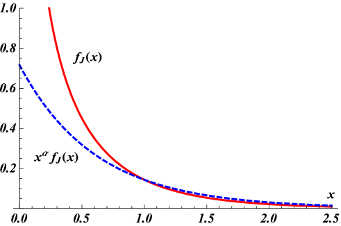
Figure 1: Gamma-like behavior of the jumps pdf $f_{J}(x)$ with $\alpha=\,^{1}/_{2},\;\beta=1,\;a=\,^{1}/_{2}$. The dashed curve shows that $f_{J}(x)=O(x^{-\alpha}),\;x\to 0^{+}$.

For later computational convenience however we prefer to give an alternative representation of this jumps distribution. Since

$$e^{-\beta w\,x}-e^{-\frac{\beta x}{a}}=\beta\,x\int_{w}^{\frac{1}{a}}e^{-\beta vx}\,dv$$

and with an exchange in the order of the integrations, the pdf (48) becomes

$$f_{J}(x) = \frac{\alpha^{2}a^{\alpha}\beta^{1-\alpha}x^{-\alpha}}{\left(1-a^{\alpha}+a^{\alpha}\log a^{\alpha}\right)\Gamma(1-\alpha)}\int_{1}^{\frac{1}{a}}\frac{dw}{w^{1+\alpha}}\int_{w}^{\frac{1}{a}}e^{-\beta vx}\,dv$$

$$= \frac{\alpha^{2}a^{\alpha}\beta^{1-\alpha}x^{-\alpha}}{\left(1-a^{\alpha}+a^{\alpha}\log a^{\alpha}\right)\Gamma(1-\alpha)}\int_{1}^{\frac{1}{a}}dv\,e^{-\beta vx}\int_{1}^{w}\frac{dw}{w^{1+\alpha}}$$

$$= \frac{\alpha^{2}a^{\alpha}\beta^{1-\alpha}x^{-\alpha}}{\left(1-a^{\alpha}+a^{\alpha}\log a^{\alpha}\right)\Gamma(1-\alpha)}\int_{1}^{\frac{1}{a}}e^{-\beta vx}\,\frac{v^{\alpha}-1}{\alpha v^{\alpha}}\,dv$$

$$= \frac{\alpha\,a^{\alpha}}{1-a^{\alpha}+a^{\alpha}\log a^{\alpha}}\int_{1}^{\frac{1}{a}}\frac{x^{-\alpha}\left(\beta\,v\right)^{1-\alpha}e^{-\beta v\,x}}{\Gamma(1-\alpha)}\,\frac{v^{\alpha}-1}{v}\,dv$$

that coincides with (46) and is a mixture of gamma laws $\mathcal{G}(1-\alpha,\beta V)$ with a random rate parameter distributed according to the pdf (47), as stated in the Remark 2 ∎

As discussed in the Section 2, the knowledge of the law of $Z(t)=X_{1}+X_{2}$ in the Proposition 5.1 also enables us to calculate the distribution of the solution (4) of the given OU equation (3) with an arbitrary initial condition $X_{0}$. In particular for a degenerate initial condition $X_{0}=x_{0},\;\bm{P}\hbox{-\emph{a.s.}}$ we will have for every $t>0$

$$X(t)\big{|}_{X_{0}=x_{0}}\,\stackrel{{\scriptstyle d}}{{=}}\,ax_{0}+X_{1}+X_{2}\qquad\quad a=e^{-bt}$$ (49)

where the distributions of $X_{1},X_{2}$ are described in detail in the Proposition 5.1. Of course the formula (7) would give access then to the transition distribution and therefore to all the details of the process.

Remark 3.

The direct extension to the bilateral finite variation setting is straightforward because every finite variation bilateral TS process can be seen as the difference of two TS processes with different parameters: as a consequence the Propositions 3.1,  4.1 and  5.1, can be easily extended to the bilateral case. As far as the simulation of such processes is concerned, this extension essentially boils down to running twice the algorithms for TS subordinators. We omit an explicit proof to avoid overloading the paper with lengthy details of routinary nature.

6 Simulation Algorithms

The simulation of TS-OU processes and CTS laws have been widely discussed in several studies (see for instance Kawai and Masuda [23, 24], Zhang [42] and Grabchack [18, 20] and the references therein) and several software packages are available for such purpose. Therefore, in this section we will only illustrate how to exactly simulate the CTS-OU and the OU-CTS processes that, although similar in names, are two rather different objects as explained in the previous sections. As far as the CTS-OU processes are concerned, our contribution is the enhancement of the simulation performance by taking advantage of the $f_{J}(x)$ reprentation (41) that, in contrast to Zhang [42], does not require any acceptance-rejection procedure. On the other hand, with regard to OU-CTS processes, we propose a new simulation procedure for the drawings from the mixture with pdf (47). At variance with the approach of Qu et al. [33], this algorithm is based on an acceptance-rejection method whose expected number of iterations before acceptance however can be made arbitrarily close to one and is therefore more efficient. In our numerical experiments we consider a time grid $t_{0},t_{1},\dots,t_{M}$, $\Delta t_{m}=t_{m}-t_{m-1}\,,\;m=1,\dots,M$ with $M$ steps.

6.1 CTS-OU processes

The simulation procedure for the generation of the skeleton of CTS process is based on the Proposition 4.1 and is summarized in the Algorithm 1.

Algorithm 1

1$X_{0}\leftarrow x$

2for  $m=1,\dots,M$ do

3     $a\leftarrow e^{-b\Delta t_{m}}$

4     $x_{1}\leftarrow X_{1}\sim\mathcal{CTS}\!\left(\alpha,\beta,c(1-a^{\alpha})\right)$

5     $n\leftarrow N_{a}\sim\mathcal{P}(\Lambda_{a})$, $\triangleright$ Generate an independent Poisson rv with $\Lambda_{a}$ in (40)

6     $u_{i}\leftarrow U_{i}\sim\mathcal{U}(0,1),i=1,\dots,n$ $\triangleright$ Generate $n$ iid uniform rv’s

7     $v_{i}\leftarrow\left(1+\frac{a^{-\alpha}-1}{\alpha}u_{i}\right)^{\frac{1}{\alpha}}$ $\triangleright$ Generate according to (43)

8     $\tilde{\beta}_{i}\leftarrow\beta\,v_{i},i=1,\dots,n$

9     $j_{i}\leftarrow J_{i}\sim\mathcal{G}(1-\alpha,\,\tilde{\beta}_{i}),i=1,\dots,n$ $\triangleright$ Generate $n$ independent gamma rv’s all with the same scale $1-\alpha$ and random rates

10     $x_{2}\leftarrow\sum_{i=1}^{n}j_{i}$

11     $X(t_{m})\leftarrow a\,X(t_{m-1})+x_{1}+x_{2}$.

12end for

We remark that when $\alpha=0$ a CTS-OU process is a compound Poisson process with a gamma stationary law whose efficient exact simulation can be found in Sabino and Cufaro Petroni [37].

6.2 OU-CTS processes

The simulation steps for the skeleton of a OU-CTS process are then summarized in the Algorithm 2.

Algorithm 2

1$X_{0}\leftarrow x$

2for  $m=1,\dots,M$ do

3     $a\leftarrow e^{-b\Delta t_{m}}$

4     $x_{1}\leftarrow X_{1}\sim\mathcal{CTS}\!\left(\alpha,\frac{\beta}{a},\frac{c(1-a^{\alpha})}{T\alpha\,b}\right)$

5     $n\leftarrow N_{a}\sim\mathcal{P}(\Lambda_{a})$, $\triangleright$ Generate an independent Poisson rv with $\Lambda_{a}$ in (40)

6     $v_{i}\leftarrow V_{i},i=1,\dots,n$ $\triangleright$ Generate $n$ iid rv’s with pdf given by Equation (47)

7     $\tilde{\beta}_{i}\leftarrow\beta\,v_{i},i=1,\dots,n$

8     $j_{i}\leftarrow J_{i}\sim\mathcal{G}(1-\alpha,\,\tilde{\beta}_{i}),i=1,\dots,n$ $\triangleright$ Generate $n$ independent generalized gamma rv’s all with the same $p$, scale $p-\alpha$ and random rates

9     $x_{2}\leftarrow\sum_{i=1}^{n}j_{i}$

10     $X(t_{m})\leftarrow a\,X(t_{m-1})+x_{1}+x_{2}$.

11end for

The sampling from a CTS law has been widely studied by several authors (see for instance Devroye [14] and Hofert [22]), and here the only non-standard step is the fifth one in the Algorithm 2, namely that allowing the generation of the jumps of the compound Poisson process of Proposition 5.1. On the other hand, as mentioned in Remark 2, these jump sizes are iid distributed rv’s following a gamma law with shape $1-\alpha$ and a random rate. Therefore the unique remaining task is to sample from a law with thr pdf $f_{V}(v)$ (47). Since however this pdf is not monotonic in $[1,\,^{1}/_{a}]$ for every value of its parameters, we first define the new rv

$$W=-\frac{\log V}{\log a}\qquad\qquad V=a^{-W}=e^{-W\log a}$$

that has now the pdf

$$f_{W}(w) = \frac{-a^{\alpha}\log a^{\alpha}}{1-a^{\alpha}+a^{\alpha}\log a^{\alpha}}\,\left(a^{-\alpha w}-1\right)$$ (50)

$$= \frac{\log a^{-\alpha}}{a^{-\alpha}-1-\log a^{-\alpha}}\,\left(e^{w\log a^{-\alpha}}-1\right)\qquad\quad 0\leq w\leq 1.$$

It is straightforward to check then that $f_{W}(w)$ is monotonic and convex in $[0,1]$ and hence one can rely on the inversion-rejection algorithm illustrated in Devroye [13] page 355. The solution that we propose here is very similar to that, and in effect consists in replacing the steps required for the sequential search of the inversion part with the method of partitioning the densities into intervals (see once again Devroye [13] page 67). We remark indeed that $f_{W}(w)$, besides being monotonic and convex, also has the following upper bound

$$\qquad\qquad f_{W}(w)\leq g(w)=G(a,\alpha)\,\bar{g}(w),\qquad\qquad\qquad 0\leq w\leq 1$$

$$G(a,\alpha)=\frac{\log a^{-\alpha}\left(a^{-\alpha}-1\right)}{2\left(a^{-\alpha}-1-\log a^{-\alpha}\right)}\,,\qquad\quad\bar{g}(w)=2\,w$$

namely it is dominated by a linear function where $G(a,\alpha)$ is the area under $g(x)$. We could therefore devise a simple acceptance-rejection procedure where $G$ should be as close to $1$ as possible because it roughly represents the number of iterations needed in the rejection algorithm. While however $G(a,\alpha)\to 1^{+}$ when $a\rightarrow 1^{-}$, unfortunately it is $G(a,\alpha)\to+\infty$ for $a\rightarrow 0^{+}$. Taking therefore $a=e^{-b\,t}$, this latter limit means that the generation of a OU-CTS process with a large $b\,t$ might either have a heavy computational cost, or potentially require a large number of simulations.

In principle we could consider only small time steps, but on the other hand the acceptance-rejection sampling can be easily improved, via the modified decomposition method elucidated in Devroye [13] page $69$, just by taking a piecewise linear dominating function $g(w)$. More precisely we partition $[0,1]$ into $L$ disjoint intervals $\mathcal{I}_{\ell}=[w_{\ell-1},w_{\ell}],\;\;\ell=1,\dots,L$,   $\bigcup_{\ell}\mathcal{I_{\ell}}=[0,1]$ with $w_{0}=0$, and then we have

$$\qquad\qquad\qquad\qquad\qquad f_{W}(w)\leq g_{L}(w)=\sum_{\ell=1}^{L}\,g_{\ell}(w)\mathds{1}_{\ell}(w),$$

$$g_{\ell}(w)=\frac{f_{W}(w_{\ell})-f_{W}(w_{\ell-1})}{w_{\ell}-w_{\ell-1}}\,w+f_{W}(w_{\ell-1}),\quad\mathds{1}_{\ell}(w)\!=\!\left\{\begin{array}[]{ll}\!\!1,&\hbox{if $w\in\mathcal{I}_{\ell}$}\\ \!\!0,&\hbox{else}\end{array}\right.\quad\ell=1,\dots,L$$

where we can also write

$$\qquad\quad g_{L}(w)=G_{L}(a,\alpha)\,\sum_{\ell=1}^{L}p_{\ell}\,\bar{g}_{\ell}(w),\qquad\quad\bar{g}_{\ell}=\frac{g_{\ell}(w)}{q_{\ell}},$$

$$q_{\ell}=\int_{\mathcal{I}_{\ell}}g_{L}(w)dw,\qquad\quad p_{\ell}=\frac{q_{\ell}}{G_{L}(a,\alpha)},\qquad\quad G_{L}(a,\alpha)=\sum_{\ell=1}^{L}q_{\ell}.$$

Apparently the $\bar{g}_{\ell}(w),\;\ell=1,\dots,L$ turn out to be piecewise linear pdf’s, while the $p_{\ell}$ constitute a discrete, normalized distribution. Increasing the number $L$ of the intervals, with given $0<a<1$ and $0<\alpha<1$, $G_{L}(a,\alpha)$ can be made arbitrary close to $1$ because it measures the trapezoidal approximation of $\int_{0}^{1}f_{W}(w)dw=1$. On the other hand the random drawing from the laws with pdf’s $\bar{g}_{\ell}(w),\;\ell=1,\dots,L$ is very simple and can be implemented via the standard routines. Denoting now with $S$ a rv with distribution $\bm{P}\left\{{S=\ell}\right\}=p_{\ell},\;\ell=1,\dots,L$, and with $Y_{\ell}$ a rv with pdf $\bar{g}_{\ell}(w)$, the Algorithm 3 summarizes the instructions needed to implement the fifth step in the Algorithm 2. We remark finally that an alternative procedure, leading to similar results, might have been some shrewd decomposition of $f_{W}(w)$ rather than of its dominating curve. However Devroye [13] at the page 70 nicely spell out the reasons why the procedure here adopted is in principle preferable.

Algorithm 3

1$s\leftarrow S$ $\triangleright$ Generate a discrete rv with $\bm{P}\left\{{S=\ell}\right\}=p_{\ell},\;\ell=1,\dots,L$

2while $u\leq\frac{f_{W}(y)}{g_{L}(y)}$ do

3     $u\leftarrow U\sim\mathcal{U}{[0,1]}$ $\triangleright$ Generate a uniform rv.

4     $y\leftarrow Y_{\ell}$ $\triangleright$ Generate a rv with pdf $\bar{g}_{\ell}(w)$

5end while

6$v\leftarrow a^{-\alpha\,y}$

7return v

Remark 4.

It is worthwhile mentioning that an alternative procedure relying on a different acceptance-rejection strategy has been proposed in Qu et al. [33]. In contrast to this last approach, however, in our algorithm $G_{L}(a,\alpha)$ can be made arbitrary close to $1$ irrespective of the value of $a$ (and of the size of the time-step), and therefore our approach turns out to be computationally more efficient.

On the other hand we can also take advantage of the interplay between the OU-CTS and the CTS-OU processes to gain an insight into the possible benefits of the different simulation strategies: from (12) we find indeed that the Lévy density of the BDLP $L(t)$ for a CTS-OU process is

$$\nu_{L}(x)=c\,T\,b\,\alpha\frac{e^{-\beta\,x}}{x^{\alpha+1}}+c\,T\,b\,\beta\frac{e^{-\beta\,x}}{x^{\alpha}}.$$ (51)

where the first term apparently provides the BDLP $L_{1}(t)$ of an OU-CTS, whereas the second one corresponds to a compound Poisson $L_{2}(t)$ (see Cont and Tankov [10] page 132). Therefore the path-wise solution (4) of our CTS-OU process is now

$$X(t)=x_{0}e^{-bt}+Z_{1}(t)+Z_{2}(t)\qquad\left\{\begin{array}[]{l}Z_{1}(t)=\int_{0}^{t}e^{-b(t-s)}dL_{1}(s)\\ Z_{2}(t)=\int_{0}^{t}e^{-b(t-s)}dL_{2}(s)\end{array}\right.$$

where $Z_{1}$ is a OU-CTS (with $Z_{1}(0)=0$) and, as shown in (36), $Z_{2}$ is a compound Poisson that can easily be simulated based on (37). On the other hand, according to the Proposition 5.1, the OU-CTS process $Z_{1}(t)$ is in its turn the sum of a (time-dependent) CTS rv $X_{1}$ and of a (time-dependent) compound Poisson rv $X_{2}$; so that ultimately a CTS-OU process with a degenerate initial condition $X_{0}=x_{0}$ – beyond being of the form (38) presented in the Proposition 4.1 – can now be seen also as the sum of four random terms: one distributed according to a CTS law, two compound Poisson rv’s and a degenerate summand. Of course the two representations coincide in distribution and, as a matter of fact, the four-terms representation reproduces again that of Qu et al. [33]; but the possible alternative simulation algorithms stemming from the four term representation, although perfectly correct, would require now the generation of three rv’s and the use of acceptance-rejection methods in addition to that needed for the sampling of a CTS distributed rv, and therefore they would turn out to be rather less efficient than the Algorithm 1.

Finally, based on Remark 2 and on the results of Qu et al. [32], we notice that for $\alpha=0$ the simulation of $V$ is here much easier because no acceptance-rejection method is required.

7 Numerical Experiments

In this section, we will assess the performance and the effectiveness of our algorithms through extensive numerical experiments. All the simulation experiments in the present paper have been conducted using Python with a $64$-bit Intel Core i5-6300U CPU, 8GB. The performance of the algorithms is ranked in terms of the percentage error relative to the first four cumulants denoted err % and defined as

$$\text{err \%}=\frac{\text{true value}-\text{estimated value}}{\text{true value}}$$

Finally, for simplicity we assume that the value of the constant time scale is $T=1$.

7.1 CTS-OU processes

Since the Lévy density on $[0,+\infty)$ of the stationary law $\mathcal{CTS}\left(\alpha,\beta,c\right)$ of a CTS-OU process with finite variation and parameters $\alpha,\beta,c$ is

$$\overline{\nu}_{X}(x)=\frac{c\,e^{-\beta x}}{x^{1+\alpha}}\qquad\quad x>0,\qquad\beta>0,\qquad 0\leq\alpha<1$$

its cumulants are (see for instance Cont and Tankov [10], Proposition 3.13)

$$c_{\overline{X},k}=\int_{0}^{+\infty}x^{k}\overline{\nu}_{X}(x)\,dx=c\,\beta^{\alpha-k}\Gamma(k-\alpha)$$ (52)

and therefore from (16) and (17) we obtain the cumulants of $X(\Delta t)$ with the degenerate initial condition $X_{0}=x_{0}$

$$c_{X,k}(x_{0},\Delta t)=x_{0}e^{-b\Delta t}\delta_{k,1}+c\,\beta^{\alpha-k}\Gamma(k-\alpha)(1-e^{-kb\Delta t})\qquad\quad k=1,2,\ldots$$ (53)

In our numerical experiments we consider a CTS-OU process with parameters $\left(b,c,\beta\right)=\left(10,0.8,1.4\right)$ whose trajectories with $\alpha\in\{0.3,0.5,0.7,0.9\}$ are displayed in Figure 2 where of course the case $\alpha=0.5$ is that of an IG-OU (inverse Gaussian) process. We remark that the sampling from an IG law can be performed via the many-two-one transformation method of Michael et al. [30], and therefore no acceptance-rejection procedure is required in Algorithm 1 to generate the skeleton of an IG-OU process.

Figure 2: Sample trajectories of CTS-OU processes with $\left(b,c,\beta\right)=\left(10,0.8,1.4\right)$ and $\alpha\in\{0.3,0.5,0.7,0.9\}$

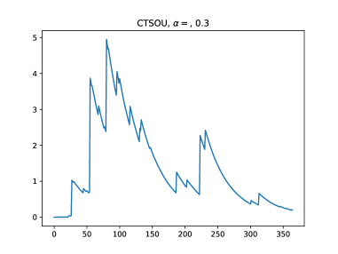
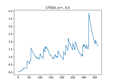
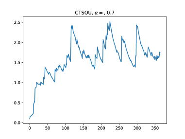
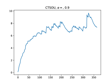
The Tables 1 and 2 compare then the true values of the first four cumulants $c_{X,k}(0,\Delta t)$ with their corresponding estimates from $10^{6}$ simulations respectively with $\Delta t=1/365$ and $\Delta t=30/365$. We can conclude therefrom that the proposed Algorithm 1 produces unbiased cumulants that are very close to their theoretical values. For the sake of brevity, we do not report the additional results obtained with different parameter settings that anyhow bring us to the same findings. Overall, from the numerical results reported in this section, it is evident that the Algorithm 1 proposed above can achieve a very high level of accuracy as well as a conspicuous efficiency.

The fact that we can easily compute the cumulants of an OU process substantiates the advantages of focusing our treatment on the law of the $a$-remainder of its stationary distribution. In addition to both the simple derivation of the transition pdf and the detailed testing of its statistical properties, we could indeed also conceive a parameter estimation procedure based on the generalized method of moments (GMM). We remark finally that the law of an $a$-remainder always is id, and therefore a simple modification of the simulation procedure presented in the Algorithm 1 could be adopted for the generation of a Lévy process whose law at time $T$ is that of the $a$-remainder of a CTS distribution.

	$c_{X,1}(0,\Delta t)$			$c_{X,2}(0,\Delta t)$			$c_{X,3}(0,\Delta t)$			$c_{X,4}(0,\Delta t)$
Algorithm 1
$\alpha$	true	MC	err %	true	MC	err %	true	MC	err %	true	MC	err %
$0.1$	$1.71$	$1.72$	$-0.6$	$2.16$	$2.18$	$-0.9$	$4.35$	$4.39$	$-0.9$	$11.85$	$11.91$	$-0.6$
$0.3$	$2.22$	$2.22$	$0.0$	$2.19$	$2.20$	$-0.7$	$3.93$	$4.00$	$-1.8$	$9.97$	$10.25$	$-2.8$
$0.5$	$3.24$	$3.24$	$0.1$	$2.28$	$2.28$	$0.3$	$3.62$	$3.63$	$-0.4$	$8.50$	$8.63$	$-1.6$
$0.7$	$5.85$	$5.85$	$-0.1$	$2.47$	$2.48$	$-0.4$	$3.40$	$3.42$	$-0.7$	$7.34$	$7.44$	$-1.3$
$0.9$	$19.89$	$19.90$	$-0.1$	$2.80$	$2.82$	$-0.7$	$3.26$	$3.29$	$-0.9$	$6.43$	$6.40$	$0.4$

Table 1: Comparing the first four true cumulants with their corresponding MC-estimated values (multiplied by $100$) obtained with $10^{6}$ simulations and $\Delta t=1/365$.

	$c_{X,1}(0,\Delta t)$			$c_{X,2}(0,\Delta t)$			$c_{X,3}(0,\Delta t)$			$c_{X,4}(0,\Delta t)$
Algorithm 1
$\alpha$	true	MC	err %	true	MC	err %	true	MC	err %	true	MC	err %
$0.1$	$3.54$	$3.60$	$-1.8$	$3.28$	$3.33$	$-1.6$	$5.04$	$5.16$	$-2.4$	$10.99$	$11.57$	$-5.3$
$0.3$	$4.60$	$4.65$	$-1.1$	$3.31$	$3.40$	$-2.8$	$4.56$	$4.73$	$-3.8$	$9.25$	$9.77$	$-5.7$
$0.5$	$6.72$	$6.81$	$-1.4$	$3.45$	$3.50$	$-1.5$	$4.20$	$4.40$	$-5.0$	$7.88$	$8.15$	$-3.4$
$0.7$	$12.12$	$12.20$	$-0.6$	$3.74$	$3.82$	$-2.1$	$3.94$	$4.05$	$-2.8$	$6.81$	$6.98$	$-2.5$
$0.9$	$41.24$	$41.28$	$-0.1$	$4.24$	$4.27$	$-0.7$	$3.78$	$3.82$	$-1.2$	$5.96$	$6.06$	$-1.6$

Table 2: Comparing the first four true cumulants with their corresponding MC-estimated values (multiplied by $10$) obtained with $10^{6}$ simulations and $\Delta t=30/365$.

7.2 OU-CTS processes

Here too we will benchmark the results of the numerical experiments against the true values of the first four cumulants of OU-CTS process at time $\Delta t$ with $X(0)=0$. From the formula (52) for the cumulants of a $\mathcal{CTS}\left(\alpha,\beta,c\right)$ distribution, and from (14) and (15) we first recover indeed the cumulants of $X(\Delta t)$ with the degenerate initial condition $X_{0}=x_{0}$

$$c_{X,k}(x_{0},\Delta t)=x_{0}e^{-b\Delta t}\delta_{k,1}+\frac{c\,(1-e^{-k\Delta t})}{Tb\,k\beta^{k-\alpha}}\,\Gamma\left(k-\alpha\right)\qquad\quad k=1,2,\ldots$$ (54)

For our simulations we consider then the same parameter settings of the previous section – $\left(b,c,\beta\right)=\left(10,0.8,1.4\right)$ – adapted to an OU-CTS process, and with $\alpha\in\{0.3,0.5,0.7,0.9\}$ we get the sample trajectories displayed in the Figure 3, where of course the case $\alpha=0.5$ is that of an OU-IG process.

Figure 3: Sample trajectories of OU-CTS processes with $\left(b,c,\beta\right)=\left(10,0.8,1.4\right)$ and $\alpha\in\{0.3,0.5,0.7,0.9\}$

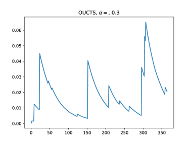
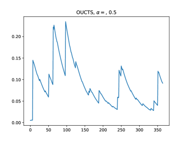
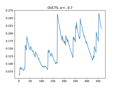
In addition to the Algorithm 2, to generate the OU-CTS processes we will consider here two approximate procedures: the first boils down to simply neglect $X_{2}$ in the Proposition 5.1; the second – in the same vein of Benth et al. [5] dealing with the normal inverse Gaussian-driven OU processes – takes advantage of the approximation of the law of $Z(t)$ in (4) with that of $e^{-k\,t}L(t)$ where $L(t)\sim\mathcal{CTS}\left(\alpha,\,^{\beta}/_{a},\,c\,t\right)$. The Tables 3 and 4 compare then the true values of the first four cumulants $c_{X,k}(0,\Delta t)$ with their corresponding estimates for $10^{6}$ simulations with $\Delta t=1/365$ and $\Delta t=30/365$; the labels $X_{1}$ only and Approximation 2 refer to the aforesaid first and second alternative procedures respectively.

From the Table 3 we can now conclude that our Algorithm 2 has the lowest percent errors, but nevertheless, in some practical situations, the errors of two other approximations could be deemed acceptable taking also into account that their computational cost is lower. In particular, the second alternative procedure outperforms the third one and its percent errors are not much higher than those of the exact method. When however the time step is larger, or equivalently when $a=e^{-b\Delta t}$ is close to $0$, the three procedures give radically different outcomes and, as it is shown in the Table 4, the two approximate methods return completely biased results. Conversely, the exact method continues to be reliable and its percent errors remain small even for the higher cumulants.

The previous state of affairs for an OU-CTS is due to the fact that $X_{2}$ in Proposition 5.1 produces only a second order effect when $\Delta t\to 0^{+}$: using indeed a Taylor expansion we find

$$\Lambda_{a}=\frac{c\Gamma(1-\alpha)b\,\beta^{\alpha}}{2T}\,(\Delta t)^{2}+o\big{(}(\Delta t)^{2}\big{)}$$

and therefore the compound Poisson $X_{2}$ has a relevant impact only when $\Delta t$ is not too small. Notice instead that this is not how a CTS-OU process behaves because from the Proposition 4.1 we see that for $\Delta t\to 0^{+}$

$$\Lambda_{a}=c\Gamma(1-\alpha)b\,\beta^{\alpha}\Delta t+o(\Delta t)$$

so that $X_{2}$ results in a first order effect and cannot be neglected even for small $\Delta t$. As mentioned above, to tackle the simulation of the random rate, Qu et al. [33] have proposed an alternative solution that is based on an acceptance rejection method again, and whose expected number of iterations before acceptance tends to $1$ for small time steps ($\Delta t\to 0^{+};\;a\rightarrow 1^{-}$); but unfortunately this value somehow deteriorates and tends to $2$ ($50\%$ of acceptance) for large time steps ($\Delta t\to+\infty;\;a\rightarrow 0^{+}$). From our previous findings we know instead that neglecting $X_{2}$ is a fair approximation for finer time grids so that the impact on the computational cost of the acceptance rejection is rather restricted. On the other hand, no matter how large the time step $\Delta t$ is, with our algorithm the expected number of iterations before acceptance can be kept as close to $1$ as possible because it depends on the accuracy of a trapezioidal approximation. Therefore, recalling also that the computational cost to generate a simple discrete rv is very low, our approach turns out to be computationally more efficient.

These observations could lead to a convenient strategy combining parameters estimation and exact simulation of the OU-CTS processes. Assuming that the data could be made available with a fine enough time-granularity (e.g. daily $t=1/365$), we could base the parameters estimation on the likelihood methods by approximating the exact transition pdf with that of a CTS law $\mathcal{CTS}\left(\alpha,\frac{\beta}{a},\frac{c\left(1-a^{\alpha}\right)}{T\alpha\,b}\right)$. However, to avoid being forced to always simulate the OU-CTS processes on a fine time-grid allowing the approximations (for instance if one needs to simulate it at a monthly granularity $t=30/365$), the generation of the skeleton of such processes will be preferably based on the exact method of the Algorthm 2.

	$c_{X,1}(0,\Delta t)$			$c_{X,2}(0,\Delta t)$			$c_{X,3}(0,\Delta t)$			$c_{X,4}(0,\Delta t)$
Algorithm 2
$\alpha$	true	MC	err %	true	MC	err %	true	MC	err %	true	MC	err %
$0.1$	$1.71$	$1.70$	$0.2$	$1.08$	$1.07$	$0.7$	$1.45$	$1.43$	$1.0$	$2.96$	$2.91$	$1.7$
$0.3$	$2.22$	$2.22$	$-0.1$	$1.09$	$1.08$	$0.9$	$1.31$	$1.27$	$3.2$	$2.49$	$2.43$	$2.5$
$0.5$	$3.24$	$3.23$	$0.2$	$1.14$	$1.15$	$-0.5$	$1.21$	$1.25$	$-3.6$	$2.12$	$2.18$	$-2.7$
$0.7$	$5.85$	$5.85$	$0.0$	$1.24$	$1.24$	$-0.4$	$1.13$	$1.16$	$-2.4$	$1.84$	$1.91$	$-4.2$
$0.9$	$19.89$	$19.88$	$0.0$	$1.40$	$1.39$	$0.6$	$1.09$	$1.06$	$2.4$	$1.61$	$1.54$	$4.2$
$X_{1}$ only
$\alpha$	true	MC	err %	true	MC	err %	true	MC	err %	true	MC	err %
$0.1$	$1.71$	$1.68$	$1.8$	$1.08$	$1.04$	$4.2$	$1.45$	$1.35$	$6.7$	$2.96$	$2.72$	$8.2$
$0.3$	$2.22$	$2.19$	$1.4$	$1.09$	$1.06$	$3.3$	$1.31$	$1.24$	$5.6$	$2.49$	$2.28$	$8.6$
$0.5$	$3.24$	$3.22$	$0.6$	$1.14$	$1.11$	$2.5$	$1.21$	$1.14$	$5.2$	$2.12$	$1.94$	$8.9$
$0.7$	$5.85$	$5.82$	$0.4$	$1.24$	$1.21$	$2.1$	$1.13$	$1.09$	$4.1$	$1.84$	$1.73$	$5.8$
$0.9$	$19.89$	$19.86$	$0.1$	$1.40$	$1.37$	$2.2$	$1.09$	$1.01$	$6.9$	$1.61$	$1.36$	$15.6$
Approximation 2
$\alpha$	true	MC	err %	true	MC	err %	true	MC	err %	true	MC	err %
$0.1$	$1.71$	$1.63$	$4.3$	$1.08$	$1.06$	$2.1$	$1.45$	$1.56$	$-7.5$	$2.96$	$3.62$	$-22.4$
$0.3$	$2.22$	$2.16$	$2.4$	$1.09$	$1.00$	$8.6$	$1.31$	$1.05$	$19.6$	$2.49$	$1.63$	$34.7$
$0.5$	$3.24$	$3.22$	$0.5$	$1.14$	$1.17$	$-2.5$	$1.21$	$1.34$	$-11.0$	$2.12$	$2.54$	$-19.7$
$0.7$	$5.85$	$5.68$	$2.8$	$1.24$	$1.16$	$6.1$	$1.13$	$0.95$	$16.3$	$1.84$	$1.37$	$25.4$
$0.9$	$19.89$	$19.58$	$1.6$	$1.40$	$1.35$	$3.8$	$1.09$	$1.04$	$3.8$	$1.61$	$1.41$	$12.5$

Table 3: Comparing the first four true cumulants with their corresponding MC-estimated values (multiplied by $1000$) obtained with $10^{6}$ simulations and $\Delta t=1/365$. The exact method uses subdivisions in $L=10$ intervals.

	$c_{X,1}(0,\Delta t)$			$c_{X,2}(0,\Delta t)$			$c_{X,3}(0,\Delta t)$			$c_{X,4}(0,\Delta t)$
Algorithm 2
$\alpha$	true	MC	err %	true	MC	err %	true	MC	err %	true	MC	err %
$0.1$	$3.54$	$3.54$	$0.1$	$1.64$	$1.65$	$-0.8$	$1.68$	$1.73$	$-2.7$	$2.75$	$2.89$	$-5.2$
$0.3$	$4.60$	$4.58$	$0.4$	$1.65$	$1.62$	$1.9$	$1.52$	$1.49$	$2.0$	$2.31$	$2.36$	$-2.1$
$0.5$	$6.72$	$6.72$	$-0.1$	$1.73$	$1.74$	$-1.0$	$1.40$	$1.43$	$-2.0$	$1.97$	$1.98$	$-0.3$
$0.7$	$12.12$	$12.15$	$-0.2$	$1.87$	$1.88$	$-0.4$	$1.31$	$1.31$	$0.6$	$1.70$	$1.63$	$4.0$
$0.9$	$41.24$	$41.22$	$0.1$	$2.12$	$2.12$	$0.2$	$1.26$	$1.25$	$0.8$	$1.49$	$1.42$	$4.6$
$X_{1}$ only
$\alpha$	true	MC	err	true	MC	err	true	MC	err	true	MC	err
$0.1$	$3.54$	$2.37$	$33.0$	$1.64$	$0.67$	$58.9$	$1.68$	$0.41$	$75.7$	$2.75$	$0.39$	$85.8$
$0.3$	$4.60$	$3.35$	$27.1$	$1.65$	$0.74$	$55.6$	$1.52$	$0.39$	$74.2$	$2.31$	$0.33$	$85.6$
$0.5$	$6.72$	$5.34$	$20.4$	$1.73$	$0.84$	$51.4$	$1.40$	$0.40$	$71.4$	$1.97$	$0.33$	$83.3$
$0.7$	$12.12$	$10.57$	$12.8$	$1.87$	$1.00$	$46.8$	$1.31$	$0.40$	$69.3$	$1.70$	$0.29$	$83.2$
$0.9$	$41.24$	$39.37$	$4.5$	$2.12$	$1.24$	$41.6$	$1.26$	$0.44$	$65.2$	$1.49$	$0.32$	$78.3$
Approximation 2
$\alpha$	true	MC	err	true	MC	err	true	MC	err	true	MC	err
$0.1$	$3.54$	$2.29$	$35.4$	$1.64$	$0.65$	$60.4$	$1.68$	$0.39$	$77.0$	$2.75$	$0.35$	$87.3$
$0.3$	$4.60$	$2.95$	$35.8$	$1.65$	$0.65$	$60.8$	$1.52$	$0.34$	$77.5$	$2.31$	$0.29$	$87.7$
$0.5$	$6.72$	$4.34$	$35.4$	$1.73$	$0.69$	$60.2$	$1.40$	$0.33$	$76.7$	$1.97$	$0.26$	$86.9$
$0.7$	$12.12$	$7.82$	$35.5$	$1.87$	$0.74$	$60.3$	$1.31$	$0.31$	$76.6$	$1.70$	$0.23$	$86.5$
$0.9$	$41.24$	$26.60$	$35.5$	$2.12$	$0.84$	$60.5$	$1.26$	$0.29$	$76.9$	$1.49$	$0.20$	$86.8$

Table 4: Comparing the first four true cumulants with their corresponding MC-estimated values (multiplied by $100$) obtained with $10^{6}$ simulations and $\Delta t=30/365$. The exact method uses subdivisions in $L=10$ intervals.

8 Conclusions

In this paper we have studied the transition laws of the tempered stable related OU processes with finite variation from the standpoint of the $a$-remainders of sd distributions: in fact, the transition law of any OU process essentially coincides with the distribution of the $a$-remainder of its stationary sd distribution. To this purpose, we first derived the Lévy triplet of the $a$-remainder of a general sd law that is then instrumental to find the representation of the transition law of tempered stable related OU processes with finite variation. We thereafter focused our attention on the CTS-OU and the OU-CTS processes: respectively those whose stationary law is a CTS distribution, and those whose BDLP is a CTS process. As already done in Zhang [43], Kawai and Masuda [23] and Qu et al. [33], we have shown that their transition law coincides with the distribution of the sum of a CTS distributed rv  (with scaled parameters), of a suitable compound Poisson rv and of a degenerate term: we accordingly also derived their path-generation algorithms.

As for the simulation of the skeleton of CTS-OU processes, our proposed procedure amounts to an improvement with respect to the existing solutions presented in Zhang and Zhang [43], Zhang [42], Kawai and Masuda [23]: indeed it does not rely on additional acceptance rejection methods other than that required to generate a CTS distributed rv. On the other hand, also the simulation procedure for a OU-CTS process is based on an acceptance rejection approach more efficient than that described in Qu et al. [33], because here the number of iterations before acceptance can be made arbitrarily close to $1$ no matter how fine we choose the time grid of the skeleton.

Although we have considered in the present paper only the CTS distributions restricted on the positive real axis, the results can be easily extended to the bilateral case and the simulation of the relative processes would be simply obtained by running twice the proposed algorithms. A further object of our future inquiries will be instead the possible extension to the $p\,$-TS related OU processes combined with the application of the algorithms recently proposed in Grabchak [19] to draw samples from $p\,$-TS laws. We remark moreover that, due to the fact that the laws of the $a$-remainders are id, our approach is also suited to build and simulate new Lévy processes via the subordination of a Brownian motion with the Lévy process generated by the $a$-remainder of a gamma and IG law, respectively (as done for instance in Gardini et al. [15, 16]).

All these algorithms would finally be especially useful for a simulation-based statistical inference, and for some financial applications like as the derivative pricing and the value-risk calculations. To this end, a possible future research line could be the study of the time reversal simulations in the spirit of some recent papers by Pellegrino and Sabino [31] and Sabino [36] relatively to the time-changed OU processes introduced in Li and Linetsky [28].

References

- [1] O. E. Barndorff-Nielsen, J. L. Jensen, and M. Sørensen. Some Stationary Processes in Discrete and Continuous Time. Advances in Applied Probability, 30(4):989–1007, 1998.
- [2] O.E. Barndorff-Nielsen. Processes of Normal Inverse Gaussian Type. Finance and Stochastics, 2(1):41–68, 1998.
- [3] O.E. Barndorff-Nielsen and N. Shephard. Non-Gaussian Ornstein-Uhlenbeck-based Models and some of their Uses in Financial Economics. Journal of the Royal Statistical Society: Series B, 63(2):167–241, 2001.
- [4] Ole E. Barndorff-Nielsen and Neil Shephard. Integrated ou processes and non-gaussian ou-based stochastic volatility models. Scandinavian Journal of Statistics, 30(2):277–295, 2003.
- [5] F.E. Benth, L. Di Persio, and S. Lavagnini. Stochastic Modeling of Wind Derivatives in Energy Markets. Risks, MDPI, Open Access Journal, 6(2):1–21, 2018.
- [6] F.E. Benth and A. Pircalabu. A non-gaussian ornstein-uhlenbeck model for pricing wind power futures. Applied Mathematical Finance, 25(1), 2018.
- [7] M. L. Bianchi, S.T. Rachev, and F.J. Fabozzi. Tempered Stable Ornstein-Uhlenbeck Processes: A Practical View. Communications in Statistics - Simulation and Computation, 46(1):423–445, 2017.
- [8] M.L. Bianchi and F.J. Fabozzi. Investigating the Performance of Non-Gaussian Stochastic Intensity Models in the Calibration of Credit Default Swap Spreads. Computational Economics, 46(2):243–273, Aug 2015.
- [9] D. M. Chung. Bessel Tempered Stable Distributions and Processes. International Journal of Applied and Experimental Mathematics, 1:1–12, 2016.
- [10] R. Cont and P. Tankov. Financial Modelling with Jump Processes. Chapman and Hall, London, 2004.
- [11] N. Cufaro-Petroni. Self-decomposability and Self-similarity: a Concise Primer. Physica A, Statistical Mechanics and its Applications, 387(7-9):1875–1894, 2008.
- [12] N. Cufaro Petroni and P. Sabino. Fast Pricing of Energy Derivatives with Mean-reverting Jump-diffusion Processes. Available at: https://arxiv.org/abs/1908.03137.
- [13] L. Devroye. Non-Uniform Random Variate Generation. Springer-Verlag, New York, 1986.
- [14] L. Devroye. Random Variate Generation for Exponential and Polynomially Tilted Stable Distributions. ACM Transactions on Modeling and Computer Simulation, 19(4), 2009. Article No. 18.
- [15] M. Gardini, P. Sabino, and E. Sasso. A bivariate normal inverse gaussian process with stochastic delay: efficient simulations and applications to energy markets, 2020. Available at www.arxiv.org.
- [16] M. Gardini, P. Sabino, and E. Sasso. Correlating Lévy Processes with Self-decomposability: Applications to Energy Markets, 2020. Available at www.arxiv.org.
- [17] M. Grabchak. Tempered Stable Distributions. Springer International Publishing, 2016.
- [18] M. Grabchak. Rejection Sampling for Tempered Lévy Processes. Statistics and Computing, 29(3):549–558, 2019.
- [19] M. Grabchak. An Exact Method for Simulating Rapidly Decreasing Tempered Stable Distributions. Available at https://arxiv.org/abs/2009.05696, 2020.
- [20] M. Grabchak. On the Simulation of General Tempered Stable Ornstein–Uhlenbeck Processes. Journal of Statistical Computation and Simulation, 90(6):1057–1081, 2020.
- [21] I. S. Gradshteyn and I. M. Ryzhik. Table of integrals, series, and products. Elsevier/Academic Press, Amsterdam, seventh edition, 2007.
- [22] M. Hofert. Sampling Exponentially Tilted Stable Distributions. ACM Transactions on Modeling and Computer Simulation, 22(1), 2012.
- [23] R. Kawai and H. Masuda. Exact Discrete Sampling of Finite Variation Tempered Stable Ornstein–Uhlenbeck Processes. Monte Carlo Methods and Applications, 17(3):279–300, 2011.
- [24] R. Kawai and H. Masuda. Infinite Variation Tempered Stable Ornstein–Uhlenbeck Processes with Discrete Observations. Communications in Statistics - Simulation and Computation, 41(1):125–139, 2012.
- [25] S.Y Kim, S.T. Rachev, L.M. Bianchi, and F.J. Fabozzi. The Modified Tempered Stable Distribution, GARCH-models and Option Pricing. Probability and Mathematical statistics, 29(1):91–117, 2009.
- [26] S.Y Kim, S.T. Rachev, L.M. Bianchi, and F.J. Fabozzi. Tempered Stable and Tempered Infinitely Divisible GARCH Models. Journal of Banking & Finance, 34(9):2096–2109, September 2010.
- [27] A.J Lawrance. Some Autoregressive Models for Point Processes. In P. Bartfai and J. Tomko, editors, Point Proceses and Queueing Problems (Colloquia Mathematica Societatis János Bolyai 24), volume 24, pages 257–275. North Holland, Amsterdam, 1980.
- [28] L. Li and V. Linesky. Time-changed Ornstein-Uhlenbeck Processes and their Applications in Commodity Derivative Models. Mathematical Finance, 24(2):289–330, 2014.
- [29] D. B. Madan and E. Seneta. The Variance Gamma (v.g.) Model for Share Market Returns. The Journal of Business, 63(4):511–24, 1990.
- [30] J. R. Michael, W. R. Schucany, and R. W. Haas. Generating random variates using transformations with multiple roots. The American Statistician, 30(2):88–90, 1976.
- [31] T. Pellegrino and P. Sabino. Enhancing least squares monte carlo with diffusion bridges: an application to energy facilities. Quantitative Finance, 15(5):761–772, 2015.
- [32] Y. Qu, A. Dassios, and H. Zhao. Exact Simulation of Gamma-driven Ornstein–Uhlenbeck Processes with Finite and Infinite Activity Jumps. Journal of the Operational Research Society, 0(0):1–14, 2019.
- [33] Y. Qu, A. Dassios, and H. Zhao. Exact Simulation of Ornstein–Uhlenbeck Tempered Stable Processes. Journal of Applied Probability, 0(0), 2021. Forthcoming.
- [34] Jan Rosinski. Tempering Stable Proceses. Stochastic Processes and their Applications, 117(6):677 – 707, 2007.
- [35] P. Sabino. Exact Simulation of Variance Gamma Related OU Proceses: Application to the Pricing of Energy Derivatives. Applied Mathematical Finance, 27(3):207–227, 2020.
- [36] P. Sabino. Forward or Backward Simulations? A Comparative Study. Quantitative Finance, 20(7):1213–1226, 2020.
- [37] P. Sabino and N. Cufaro Petroni. Gamma Related Ornstein–Uhlenbeck Processes and their Simulation. Journal of Computational Statistics and Simulation Finance, 2020. Forthcoming.
- [38] K. Sato. Lévy Processes and Infinitely Divisible Distributions. Cambridge U.P., Cambridge, 1999.
- [39] W. Schoutens. Lévy Proceses in Finance: Pricing Financial Derivatives. John Wiley and Sons Inc, Chichester, 2003.
- [40] E. Taufer and N. Leonenko. Simulation of Lévy-driven Ornstein–Uhlenbeck Processes with Given Marginal Distribution. Computational Statistics & Data Analysis, 53(6):2427 – 2437, 2009. The Fourth Special Issue on Computational Econometrics.
- [41] S. J. Wolfe. On a Continuous Analogue of the Stochastic Difference Equation . Stochastic Processes and their Applications, 12(2):301–312, 1982.
- [42] S. Zhang. Exact Simulation of Tempered Stable Ornstein–Uhlenbeck Proceses. Journal of Statistical Computation and Simulation, 81(11):1533–1544, 2011.
- [43] S. Zhang and X. Zhang. Exact Simulation of IG-OU Proceses. Methodology and Computing in Applied Probability, 10:1573–7713, 2008.