Principal Component Analysis and Factor Analysis for Feature Selection in Credit Rating

Abstract

The credit rating is an evaluation of a company’s credit risk that values the ability to pay back the debt and predict the likelihood of the debtor defaulting. There are various features influencing credit rating. Therefore, it is essential to select substantive features to explore the main reason for credit rating change. To address this issue, this paper exploited Principal Component Analysis and Factor Analysis as feature selection algorithms to select important features, summarized the similar features together, and obtained a minimum set of features for four sectors, Financial Sector, Energy Sector, Health Care Sector, Consumer Discretionary Sector. This paper used two data sets, Financial Ratio and Balance Sheet, with two mappings, Detailed Mapping, and Coarse Mapping, converting the target variable(credit rating) into categorical variable. To test the accuracy of credit rating prediction, Random Forest Classifier was used to test and train feature sets. The results showed that the accuracy of Financial Ratio feature sets was higher than that of Balance Sheet feature sets. In addition, Factor Analysis can reduce the number of features significantly to obtain almost the same accuracy that can decrease dramatically the time spent on analyzing data; we also summarized seven dominant factors and ten dominant factors affecting credit rating change in Financial Ratio and Balance Sheet by utilizing Factor Analysis, respectively, which can explain the reason of credit rating change better.

1 Introduction

As financial markets become more complex and borrowers become more diverse, investors and regulators increasingly rely on professional and authoritative credit rating agencies’ opinions. Credit rating is an assessment of a potential debtor (individual, enterprise, company, or government), predicting its ability to repay debt and an implicit prediction of the possibility of default by the debtor. Credit rating refers to assessing qualitative and quantitative information of potential debtors by credit rating agencies, including information provided by debtors and other non-public information obtained by analysts of credit rating agencies. Credit rating evaluation is a complex process, which considers many factors to assign a corresponding level to the enterprise. Therefore, it is necessary to hire domain experts to conduct evaluations, but such assessments are expensive. At present, scholars mainly use three methods to study corporate credit: statistical methods(Regression Analysis, Discriminant analysis, Bayesian analysis)[1]-[3], non-statistical methods(Random Forest, Support Vector Machine, Neural Network)[4]-[6], and combined methods[7]. Non-statistical methods are the most common use, and people usually use Random Forest to select important features that significantly impact the credit rating, then train and test the data set to predict the accuracy of corporate credit rating. However, in our studies, we want to exploit other methods not usually used to analyze the credit rating. Therefore we utilized Principal Component Analysis and Factor Analysis to select important features, trained and tested them 100 times by using Random Forest Classifier, recorded the average prediction accuracy of credit rating. Besides, we also classify the features to reduce dimension for our high dimensional data and find out the latent factors that create a commonality.

Objectives. This work aims to select important features via Principal Component Analysis and Factor Analysis, and sort the top 20 features as the feature data sets, respectively. Simultaneously, we also use a machine learning model random forest to train and test the data sets and compare which method can better choose the features that impact the credit rating. Finally, we conclude the main causes that contribute to the corporate credit change.

Contributions. Following are the major contributions of this paper:

• We compared the Principal Component Analysis and Factor Analysis, which both identify patterns in the correlations between variables. We optimized the sorting method of these two techniques, and selected the top 20 important features as feature data sets.Then we trained and tested data sets to make prediction by utilizing Random Forest. Then we found that Factor Analysis needs fewer features than Principal Component Analysis to achieve the same accuracy(above 95%), which reduces the time spent on data analysis to improve computational efficiency.

• We summarized similar features via Factor Analysis to determine the latent factors that explain one public aspect, and better illustrate the reason for credit rating change. For the data sets of Financial Ratio and Balance Sheet, there were seven factors and ten factors influencing the corporation credit, respectively.

The rest of the paper is described below. We present some related work in Section 2. We interpret data sets in Section 3. We introduce models and algorithms in section 4. We implement our model and show the prediction results in Section 5.We discuss the experimental results in section 6.We extract dominant factors influencing the credit rating via Factor Analysis in section 7. Finally, we draw a conclusion in section 8.

2 Related Work

Oricchi et al.[8]described a proprietary SME credit rating model and found that the model’s accuracy depends on the integrity of accounting information and behavioral information. Petropoulos et al.[9]proposed an implicit Student’s t-test Markov model to calculate credit scores. Experimental results showed that the credit rating system can effectively predict corporate credit ratings. Abiyev[10]proposed a fuzzy neural network (FNN) credit rating model to analyze corporation credit rating and evaluate its effectiveness.

Arora et al.[11]used the random forest to classify credit indicators, and the results show that the random forest model had an excellent classification effect. Yeh et al.[12]combined random forest and rough set theory to extract useful credit rating information. Jiang et al.[13]proposed a support vector machine model based on Mahalanobis distance and applied it to credit risk assessment. Experimental results show that the model can be successfully used for large-scale credit risk assessment problems and had good risk assessment capabilities.

Tansel et al.[14] used a multi-objective credit evaluation model to evaluate corporate credit and found that the multi-objective model can accurately assess corporate risks. Addo et al.[15]established a binary classifier model to predict the default probability of corporate loans and select the top ten important features that affected corporate credit ratings. The final experimental results showed that the model of the layered artificial neural network was more stable. Nehrebecka[16]used logistic regression and support vector machines to assess the credit risk of non-financial companies and found that the discriminatory logistic regression model was significantly different from the support vector machine. The logistic regression model had a higher credit risk prediction rate. Angilella et al.[17]proposed a multi-criteria credit risk model called ELECTRE-TRI to identify corporate risk categories. Hajek et al.[18]evaluated several automatic classification methods for credit rating evaluation, using a feature selection process to improve the accuracy of classification results of credit rating indicators.

3 Data

This paper uses two data sets as feature sets, Financial Ratio and Balance Sheet. Data was obtained from Wharton Research Data Services(WRDS) Database for all the S&P companies. Every sector has its own operating ways and characteristics in a company and has different effect on the credit rating of a company, Therefore, we chose specifically four typical sectors, Financial Sector, Energy Sector, Health Care Sector, Consumer Discretionary Sector. Because the type of credit rating was character variable, we needed to convert it into categorical variable with two mappings, Detailed Mapping and Coarse Mapping.The mappings were shown in Table 3.1, Table 3.2. Finally, Financial Ratio and Balance Sheet combined with two mappings to form four four data sets in every sector. The results were shown in Table 3.3.

Table 3.1: Detailed Mapping

Rating	Mapping	Rating	Mapping
AAA	1	BB-	12
AA+	2	B+	13
AA	3	B	14
AA-	4	B-	15
A+	5	CCC+	16
A	6	CCC	17
A-	7	CCC-	18
BBB+	8	CC	19
BBB	9	C	20
BBB-	10	RD	21

Table 3.2: Coarse Mapping

Rating	Mapping	Rating Description
AAA	1	Prime
AA+, AA, AA-	2	High Grade
A+,A,A-	3	Upper Medium Grade
BBB+. BBB .BBB-	4	Lower Medium Grade
BB+, BB. BB-	5	N on-Investment Grade Speculative
B+, B. B-	6	Highly Speculative
CCC+, CCC, CCC-	7	Substantial Risks ,
CC	8	Extremely Speculative
C	9	Default Imminent
RD, SD, D	10	In Default

Table 3.3: Dataset

	Data 1	Data 2	Data 3	Data 4
Data	Financial Ratio+ Detailed Mapping	Financial Ratio+ Coarse Mapping	Balance Sheet+ Detailed Mapping	Balance Sheet+ Coarse Mapping

4 Algorithm

4.1 Algorithm 1

Principal Component Analysis (PCA) using the idea of dimension reduction (linear transformation), a set of variables of possibly related are converted into a set of values of linearly uncorrelated variables (principal component) under the premise of less loss of information.The first principal component has the largest possible variance (taking into account the variability of the data), and each subsequent component has the highest possible variance under the constraint of orthogonal with the previous component.The resulting vectors (each of which is a linear combination of variables and contain n variables) are unrelated orthogonal basis sets. Each principal component is a linear combination of the original variables, and the principal components are not related to each other. In general, people select principal components with cumulative proportion of variance more than 85% because most of information is included.

The top reasons for Principal component analysis are:

• There are same numbers of variables and components in PCA. It can reduce the numbers of components if we just extract the components with variance cumulative proportion more than 85% that makes the follow-up analysis easier.

• The objective economic phenomenon is scientifically evaluated by calculating the score of the comprehensive principal component function.

• It focuses on the comprehensive evaluation of the influence of information contribution.

$$\begin{split}X_{1}&=a_{11}F_{1}+a_{12}F_{2}+\cdots+a_{1n}F_{n}\\ X_{2}&=a_{21}F_{1}+a_{22}F_{2}+\cdots+a_{2n}F_{n}\\ \cdots\\ X_{n}&=a_{n1}F_{1}+a_{n2}F_{2}+\cdots+a_{nn}F_{n}\end{split}$$ (1)

$X_{n}$ is the $n_{th}$ features. $F_{n}$ is the $n_{th}$ components. $a_{nn}=\sqrt{\lambda_{n}}e_{nn}$ is the loadings of components . ${\lambda_{n}}$ is the variance of $n_{th}$ component(also eigenvalue). ${\mid\mid e_{n}\mid\mid=1}$ is the eigenvector of $n_{th}$ component.

Before performing the PCA, we must standardize data to avoid the impact of the unit different.And in this standardized data set, the eigenvectors are unit eigenvectors. Therefore, we can regard ${e_{ni}}^{2}$ as the proportion of variance of $i_{th}$ feature of $n_{th}$ component .We select components with cumulative proportion of variance more than 85%.
( count: the number of components when cumulative proportion of variance is more than 85 %)

$$\begin{split}X_{1}&=a_{11}F_{1}+a_{12}F_{2}+\cdots+a_{1count}F_{count}\\ X_{2}&=a_{21}F_{1}+a_{22}F_{2}+\cdots+a_{2count}F_{count}\\ \cdots\\ X_{n}&=a_{n1}F_{1}+a_{n2}F_{2}+\cdots+a_{ncount}F_{count}\end{split}$$ (2)

The loadings of PCA represent the relationship between components and features.The higher the loading, the more the relationship between the two variables. Therefore, we consider adding the loadings of every component of each feature to get the loading scores that represents the extent to which features affect . Then the feature set is sorted in the decreasing order of components scores.In every iteration,the features from this set are added one in order at a time, while maintaining the order, to form the data set on which the Random Forest Classifier is trained and tested on and the accuracy of each iteration is recorded.

There are positive and negative loadings that means the loadings have positive or negative effect on components. The added scores would be counteracted if the features had positive and negative loadings that we cannot test the importance of features. To avoid this case, we propose two algorithms :

$$\begin{split}Algorithm1:Score_{i}=&\sum^{count}_{j=1}\mid a_{ij}\mid=\mid\sqrt{\lambda_{1}}e_{i1}\mid+\mid\sqrt{\lambda_{2}}e_{i2}\mid\\ +&\cdots+\mid\sqrt{\lambda_{count}}e_{icount}\mid\end{split}$$ (3)

$$\begin{split}Algorithm2:Score_{i}=\sum^{count}_{j=1}a_{ij}^{2}={\lambda_{1}}e_{i1}^{2}+{\lambda_{2}}e_{i2}^{2}+\cdots+{\lambda_{count}}e_{icount}^{2}\end{split}$$ (4)

Algorithm 1 is to add the absolute value of loading of every component of each features,the Algorithm 2 is to add the square of loading. They all can avoid positive and negative offsetting and represent that features have effect on components.In order to figure out which algorithm is better,we test the accuracy of the credit rating change of Financial Data and Balance Sheet.

Figure 4.1: Algorithm Comparison in Detailed Mapping

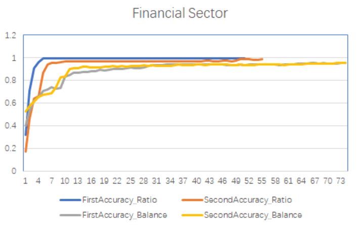
(a) Financial Sector+Detailed Mapping

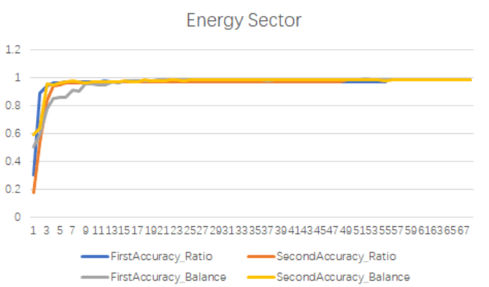
(b) Energy Sector+Detailed Mapping

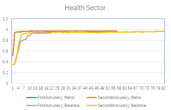
(c) Health Sector+Detailed Mapping

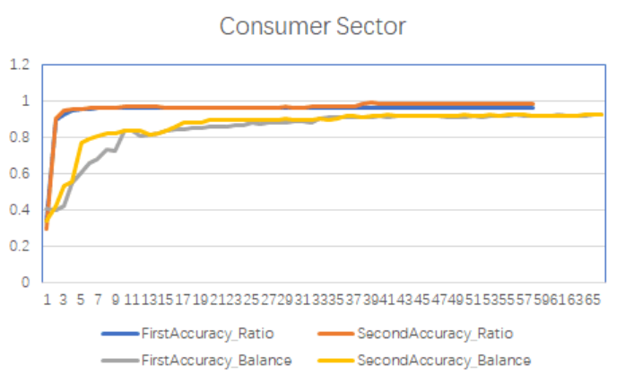
(d) Consumer Sector+Detailed Mapping

Figure 4.2: Algorithm Comparison in Coarse Mapping

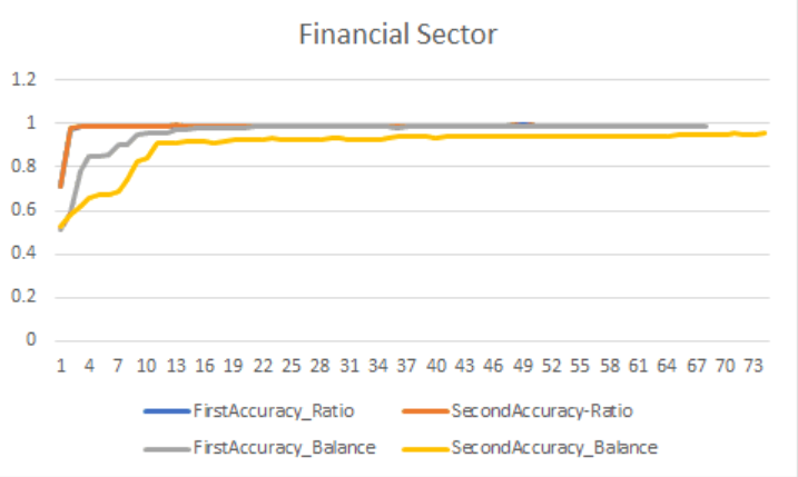
(a) Financial Sector+Coarse Mapping

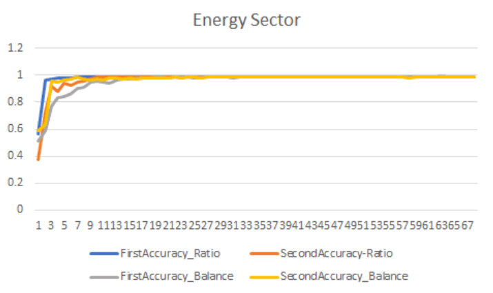
(b) Energy Sector+Coarse Mapping

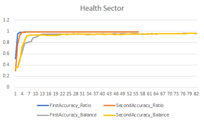
(c) Health Sector+Coarse Mapping

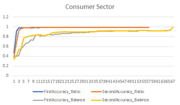
(d) Consumer Sector+Coarse Mapping

From Figure 4.1, 4.2, the blue and gray line show the accuracy of algorithm 1 in Financial Ratio and Balance Sheet respectively;orange and yellow line display the accuracy of algorithm 2 in Financial Ratio and Balance Sheet respectively.In Financial Ratio, there is slight difference between these two algorithms in four sectors. In Balance Sheet,yellow line (algorithm 2) is always above the gray line(algorithm 1) that means the accuracy of algorithm 2 is more accurate than that of algorithm 1 in four sectors.

However, the numbers of selected features for four data sets in every sector are different from each other because we select the features with Chi-square p-value less than 0.05 as final feature sets for four data sets in every sector. So we try to test the accuracy with the same numbers. From Figure 4.1, 4.2 ,most accuracy curves tent to steady when the number is 20 or more. We calculate the average accuracy of the top 20 features by utilizing Random Forest that trained and tested the accuracy of feature sets for 100 times. The results are shown in Table 4.4, Table 4.5, Table 4.6, Table 4.7.

Table 4.4: Accuracy for Financial Sector

	Financial Raio Detailed Mapping	Balance Sheet Detailed Mapping	Financial Ratio Coarse Mapping	Balance Sheet Coarse Mapping
Avg.Test Accuracy Accuracy with Algorithm 1 using The Top 20 Features	0.97169	0.87244	0.98999	0.8964
Avg.Test Accuracy Accuracy with Algorithm 2 using The Top 20 Features	0.97577	0.92332	0.98989	0.9274

Table 4.5: Accuracy for Energy Sector

	Financial Raio Detailed Mapping	Balance Sheet Detailed Mapping	Financial Ratio Coarse Mapping	Balance Sheet Coarse Mapping
Avg.Test Accuracy Accuracy with Algorithm 1 using The Top 20 Features	0.97271	0.90403	0.98915	0.98205
Avg.Test Accuracy Accuracy with Algorithm 2 using The Top 20 Features	0.97035	0.91974	0.98947	0.98064

Table 4.6: Accuracy for Health Sector

	Financial Raio Detailed Mapping	Balance Sheet Detailed Mapping	Financial Ratio Coarse Mapping	Balance Sheet Coarse Mapping
Avg.Test Accuracy Accuracy with Algorithm 1 using The Top 20 Features	0.97083	0.86841	0.99001	0.95187
Avg.Test Accuracy Accuracy with Algorithm 2 using The Top 20 Features	0.97288	0.93562	0.99035	0.93103

Table 4.7: Accuracy for Consumer Sector

	Financial Raio Detailed Mapping	Balance Sheet Detailed Mapping	Financial Ratio Coarse Mapping	Balance Sheet Coarse Mapping
Avg.Test Accuracy Accuracy with Algorithm 1 using The Top 20 Features	0.96281	0.80097	0.98614	0.86128
Avg.Test Accuracy Accuracy with Algorithm 2 using The Top 20 Features	0.96734	0.93562	0.99035	0.93103

From Table 4.4, Table 4.5, Table 4.6, Table 4.7, most accuracy of Algorithm 2 is higher than that of algorithm 1 in four sectors. Therefore, algorithm 2 in this part is designed for the final Algorithm 1.After obtaining the final algorithm 1, a summary of this algorithm is shown in Figure 4.3.

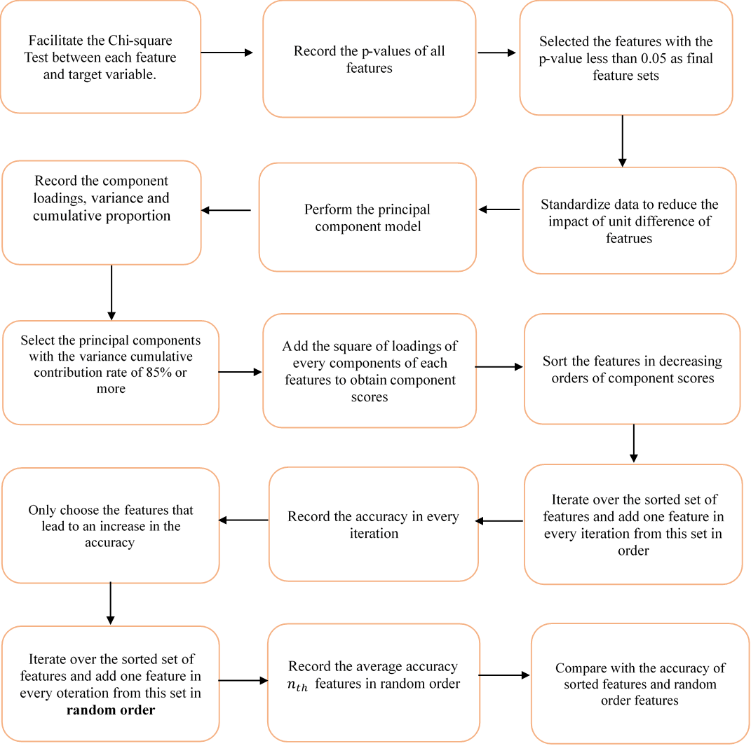
Figure 4.3: Flowchart for Algorithm 1

4.2 Algorithm 2

Factor analysis is to identify the underlying relationships between measured variables. And Factor analysis is related to principal component analysis (PCA), but the two are not identical.Factor Analysis is based on the idea of dimension reduction and the study of the dependence within the correlation matrix of the original variables, some variables with complex relationships are expressed as a linear combination of a small number of common factors and special factors that only work on one variable.In this algorithm, we try to summarize the similar features together to extract common factors that can interpret features better.

The top reasons for Factor analysis are:

• Factor analysis make the factor better explained by exploiting factor rotation. The factor analysis is more dominant in the interpretation of the principal component.

• Factor analysis is not to delete original variables ,but the information of the original variable is recombined to find a common factor affecting the target variable and simplify data.

Before performing Factor Analysis, feature set must be tested by KMO and Bartlett’s Test to examine whether the data is suitable for factor analysis.

The Kaiser-Meyer-Olkin (KMO) test measures the applicability of our data to factor analysis. The test measures sampling adequacy for each variable in the model and for the complete model.KMO values less than 0.6 indicate the sampling is not adequate that factor analysis should not be taken.

Bartlett’s Test of Sphericity is based on the correlation coefficient matrix. Its null hypothesis correlation coefficient matrix is a unit array, that is, all the elements of the diagonal of the correlation coefficient matrix are 1, and all the non-diagonal elements are zero. The statistics of Bartlett’s Test of Sphericity is derived from the determinant of the correlation coefficient matrix.If the value is large, and the corresponding concomitant probability value is less than the specified significant level, the null hypothesis is rejected, indicating that the correlation coefficient matrix is not a unit array, there is a correlation between the original variables. Small p-value (less than 0.05) of the significance level indicate that a factor analysis may be useful with data.

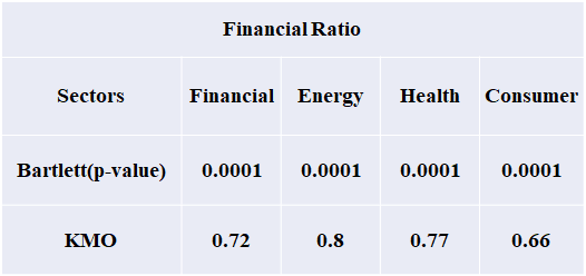
(a) Financial Ratio

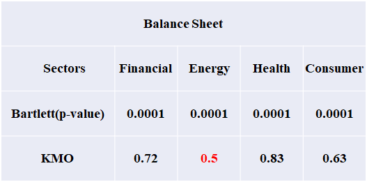
(b) Balance Sheet

Figure 4.4: KMO and Bartlett’s Test

From Figure 4.4, almost all the p-values of Bartlett’s Test are less than 0.05 and KMO vaules are more than 0.6 in four sectors in Financial Ratios and Balance Sheet except for Energy Sector in Balance Sheet.

After performing the Factor Analysis to get the rotated loadings, the features with loadings more than 0.5 are selected and the features are deleted if their loadings with less than 0.5. The feature represents the factor that its loading is maximum if they have two or more loadings more than 0.5. Because the factors are unrelated to each other, each feature can be only included by one factor,there are no same features between factors. The loading of features of factor means that have psitive or negative effect on factor and there is first factor,second factor and so on with their effects gradually weakening. According to the principle of priority of the first factor , the features of each factor are sorted according to the absolute value of loadings within first factor and then second factor and so on. For example, if first factor includes three features, their order are 1,2,3; then second factors has four features,their order are 4,5,6,7 and so on. To obtain this sorted set, the algorithm 2 is proposed. If there are m factors, feature A is included by the $j_{th}$ factor, the absolute value of loading of A plus (m-j+1) to get factor scores. It means that absolute value of loadings of the features of first factor plus highest score m, that of the second factor plus second highest score (m-1),that of the $j_{th}$ factor plus score (m-j+1) and so on. Then the feature set is sorted in the decreasing order of added scores. In every iteration,the features from this set are added one in order at a time, while maintaining the order, to form the data set on which the Random Forest Classifier is trained and tested on and the accuracy of each iteration is recorded. A summary of this algorithm is shown in Figure 4.5.

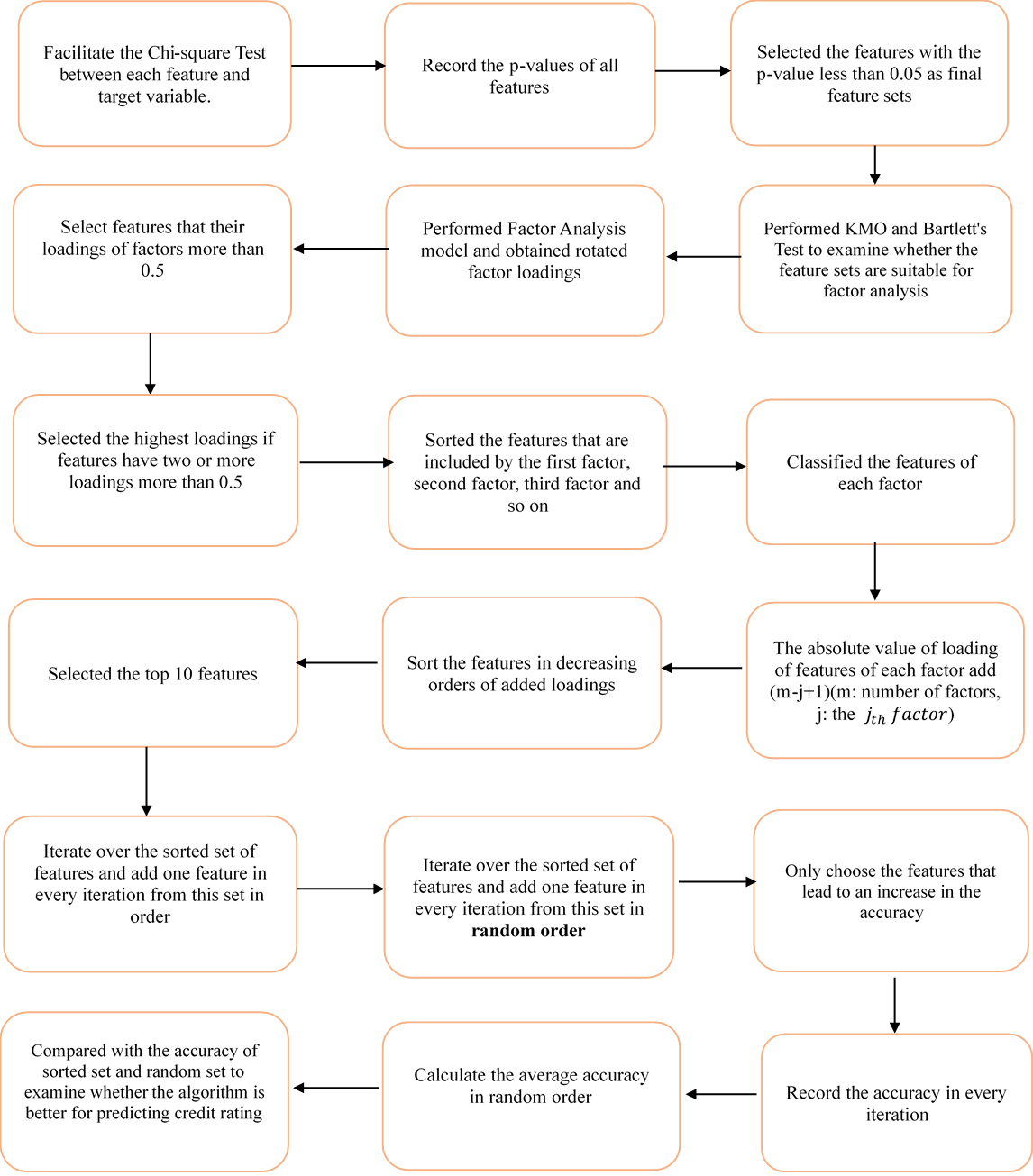
Figure 4.5: Flowchart for Algorithm 2

5 Prediction Results

In Algorithm 1, the components with cumulative variance proportion more than 85% were selected as final principal components.The number of component was shown in Table 5.1. In Algorithm 2, the factors with cumulative variance proportion more than 85% were selected as final factors. The number of factor was shown in Table 5.2.

In this section, the results for both the algorithms will be summarized according to sectors. We compared the accuracy of the top 20 features selected by Algorithm 1 and the accuracy of the features selected by Algorithm 2. These two feature sets were trained and tested for 100 times by utilizing Random Forest Classifier and the average accuracy was recorded. The results were shown in Table 5.3, Table 5.4, Table 5.5, Table 5.6.

Table 5.1: The Number of Component for Algorithm 1

	Financial Raio Detailed Mapping	Financial Ratio Coarse Mapping	Balance Sheet Detailed Mapping	Balance Sheet Coarse Mapping
Financial Sector	22	22	33	32
Energy Sector	18	18	22	21
Health Sector	22	22	29	32
Consumer Sector	28	29	28	28

Table 5.2: The Number of Factors for Algorithm 2

	Financial Raio Detailed Mapping	Financial Ratio Coarse Mapping	Balance Sheet Detailed Mapping	Balance Sheet Coarse Mapping
Financial Sector	10	10	15	14
Energy Sector	8	8	NA	NA
Health Sector	11	10	11	13
Consumer Sector	11	11	13	12

Table 5.3: Accuracy Results for Financial Sector

	Financial Raio Detailed Mapping	Balance Sheet Detailed Mapping	Financial Ratio Coarse Mapping	Balance Sheet Coarse Mapping
Avg.Test Accuracy Accuracy with Algorithm 1 using The Top 20 Features	0.97577	0.92332	0.98989	0.9274
Avg.Test Accuracy Accuracy with Algorithm 2	0.97465	0.92331	0.98983	0.95227
Avg.No feature Selection	0.97712	0.92766	0.99203	0.96721

Table 5.4: Accuracy Results for Energy Sector

	Financial Raio Detailed Mapping	Balance Sheet Detailed Mapping	Financial Ratio Coarse Mapping	Balance Sheet Coarse Mapping
Avg.Test Accuracy Accuracy with Algorithm 1 using The Top 20 Features	0.97035	0.91974	0.98947	0.98064
Avg.Test Accuracy Accuracy with Algorithm 2	0.96859	NA	0.98831	NA
Avg.No feature Selection	0.97253	0.93115	0.99027	0.98647

Table 5.5: Accuracy Results for Health Sector

	Financial Raio Detailed Mapping	Balance Sheet Detailed Mapping	Financial Ratio Coarse Mapping	Balance Sheet Coarse Mapping
Avg.Test Accuracy Accuracy with Algorithm 1 using The Top 20 Features	0.97288	0.93562	0.99035	0.93103
Avg.Test Accuracy Accuracy with Algorithm 2	0.97363	0.93091	0.99081	0.96093
Avg.No feature Selection	0.97402	0.94367	0.99112	0.96389

Table 5.6: Accuracy Results for Consumer Sector

	Financial Raio Detailed Mapping	Balance Sheet Detailed Mapping	Financial Ratio Coarse Mapping	Balance Sheet Coarse Mapping
Avg.Test Accuracy Accuracy with Algorithm 1 using The Top 20 Features	0.96734	0.93562	0.99035	0.93103
Avg.Test Accuracy Accuracy with Algorithm 2	0.96784	0.93091	0.99081	0.96093
Avg.No feature Selection	0.96836	0.94367	0.99112	0.96389

6 Discussion

We can see from Table 5.3, 5.4, 5.5, 5.6 , they showed the similar results in term of the accuracy of Algorithms. However,the number of selected features by them are different. For all the original feature sets,the features with the p-value less than 0.05 were selected by exploiting Chi-square Test. Algorithm1 was to add the loading square of every component for each features as component scores of each features and sort the features according to the compnent scores,it did not need to delete features.Therefore the number of feature sets of Algorithm 1 was equal to that of Chi-Suqare Test. Algorithm 2 was to delete features that had no loadings with more than 0.5 and sort the deleted feature sets. Therefore the number of feature sets of Algorithm 2 was not equal to that of Chi-Suqare Test.The results are shown in Table 6.1, 6.2, 6.3 , 6.4.

Table 6.1: The Number of original Features

	Financial Raio Detailed Mapping	Financial Ratio Coarse Mapping	Balance Sheet Detailed Mapping	Balance Sheet Coarse Mapping
Financial Sector	52	52	101	101
Energy Sector	57	57	111	111
Health Sector	59	59	116	116
Consumer Sector	58	58	103	103

Table 6.2: The Number of Features selected by Chi-Square Test

	Financial Raio Detailed Mapping	Financial Ratio Coarse Mapping	Balance Sheet Detailed Mapping	Balance Sheet Coarse Mapping
Financial Sector	51	50	76	74
Energy Sector	54	55	71	68
Health Sector	57	56	75	82
Consumer Sector	58	57	73	66

Table 6.3: The Number of Features for Alogorithm 1

	Financial Raio Detailed Mapping	Financial Ratio Coarse Mapping	Balance Sheet Detailed Mapping	Balance Sheet Coarse Mapping
Financial Sector	51	50	76	74
Energy Sector	54	55	71	68
Health Sector	57	56	75	82
Consumer Sector	58	57	73	66

Table 6.4: The Number of Features selected for Alogorithm 2

	Financial Raio Detailed Mapping	Financial Ratio Coarse Mapping	Balance Sheet Detailed Mapping	Balance Sheet Coarse Mapping
Financial Sector	31	31	52	50
Energy Sector	37	38	NA	NA
Health Sector	36	35	52	57
Consumer Sector	29	30	48	43

From Table 6.1, Table 6.2, Table 6.3 , Table 6.4 , the number of feature sets of Algorithm 1 was equal to that of Chi-Suqare Test. The number of features selected by Algorithm 2 was less than that of Chi-square Test. The features sets were sorted in decreasing order of components scores/factors scores and were carried out the iteration adding one feature in order in every time . We can obtain the minimum number of features when the accuracy curves became steady.To examine whether the sorted features better,the random order feature of every data set also did this iteration and repeated 10 times(each time a feature set formed a new random feature set) and the average accuracy of $n_{th}$ feature is recorded. The accuracy of comparison plot about sorted feature sets and random feature sets was displayed in Figure 6.1, 6.2, 6.3, 6.4, 6.5, 6.6, 6.7, 6.8.

Table 6.5: The Number of Features Shortilised by Algorithm 1

	Financial Raio Detailed Mapping	Financial Ratio Coarse Mapping	Balance Sheet Detailed Mapping	Balance Sheet Coarse Mapping
Financial Sector	5	12	54	14
Energy Sector	10	10	19	19
Health Sector	6	8	66	8
Consumer Sector	33	8	50	40

Table 6.6: The Number of Features Shortilised by Algorithm 2

	Financial Raio Detailed Mapping	Financial Ratio Coarse Mapping	Balance Sheet Detailed Mapping	Balance Sheet Coarse Mapping
Financial Sector	5	8	21	10
Energy Sector	8	13	NA	NA
Health Sector	9	18	13	13
Consumer Sector	7	13	32	37

Table 6.7: The Number of Random Features Shortilised by Algorithm 1

	Financial Raio Detailed Mapping	Financial Ratio Coarse Mapping	Balance Sheet Detailed Mapping	Balance Sheet Coarse Mapping
Financial Sector	11	14	66	19
Energy Sector	8	7	34	34
Health Sector	8	12	48	17
Consumer Sector	38	10	57	45

Table 6.8: The Number of Random Features Shortilised by Algorithm 2

	Financial Raio Detailed Mapping	Financial Ratio Coarse Mapping	Balance Sheet Detailed Mapping	Balance Sheet Coarse Mapping
Financial Sector	6	9	47	39
Energy Sector	8	13	NA	NA
Health Sector	8	17	49	49
Consumer Sector	6	11	36	34

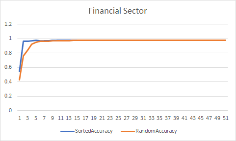
(a) Financial Sector

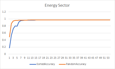
(b) Energy Sector

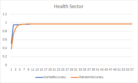
(c) Health Sector

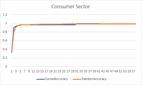
(d) Consumer Sector

Figure 6.1: Feature number in Financial Ratio Detailed Mapping for Algorithm 1

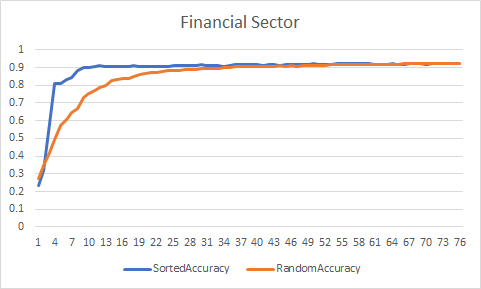
(a) Financial Sector

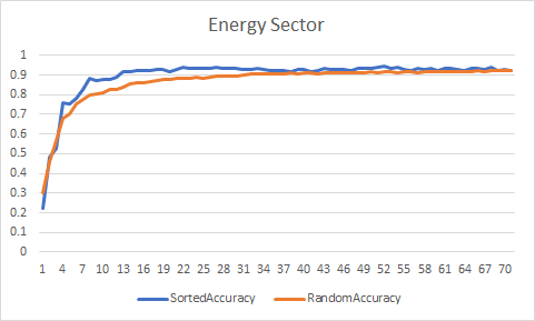
(b) Energy Sector

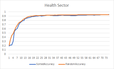
(c) Health Sector

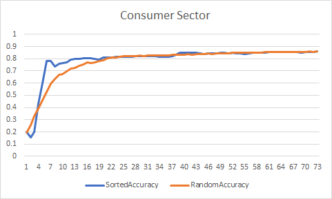
(d) Consumer Sector

Figure 6.2: Feature Number in Balance Sheet Detailed Mapping for Algorithm 1

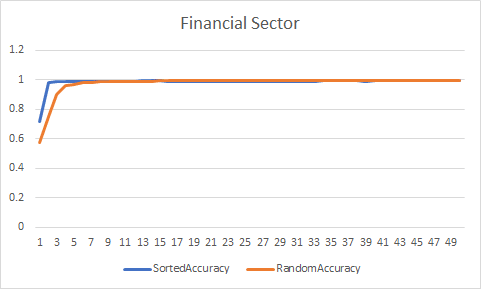
(a) Financial Sector

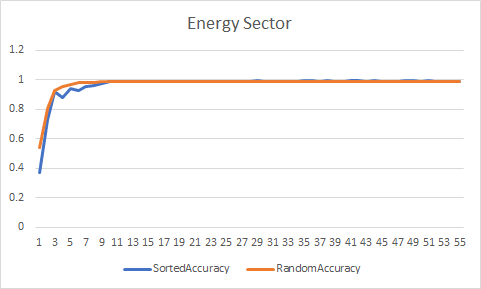
(b) Energy Sector

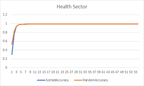
(c) Health Sector

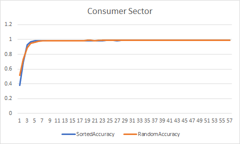
(d) Consumer Sector

Figure 6.3: Feature Number in Financial Ratio Coarse Mapping for Algorithm 1

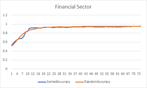
(a) Financial Sector

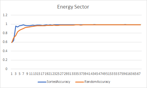
(b) Health Sector

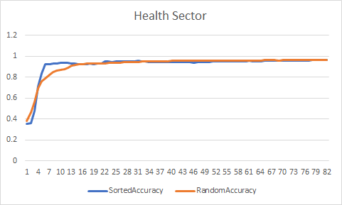
(c) Financial Sector

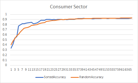
(d) Health Sector

Figure 6.4: Feature Number in Balance Sheet Coarse Mapping for Algorithm 1

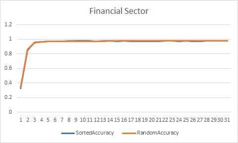
(a) Financial Sector

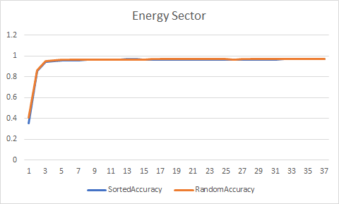
(b) Energy Sector

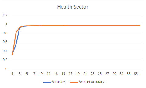
(c) Health Sector

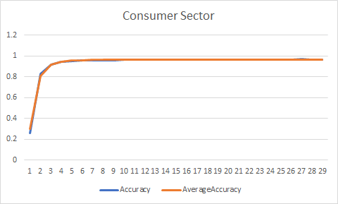
(d) Consumer Sector

Figure 6.5: Feature number in Financial Ratio Detailed Mapping for Algorithm 2

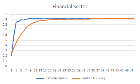
(a) Financial Sector

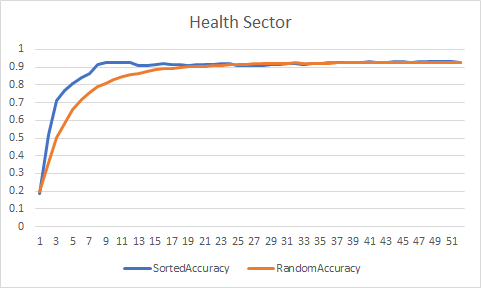
(b) Health Sector

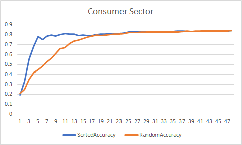
(c) Consumer Sector

Figure 6.6: Feature Number in Balance Sheet Detailed Mapping for Algorithm 2

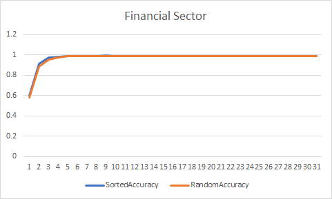
(a) Financial Sector

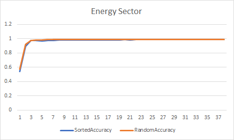
(b) Energy Sector

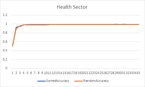
(c) Health Sector

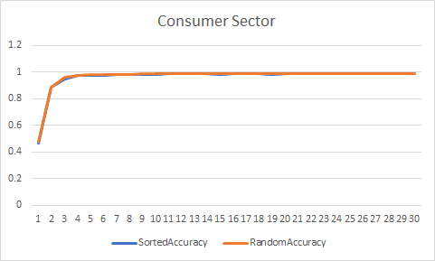
(d) Consumer Sector

Figure 6.7: Feature number in Financial Ratio+Coarse Mapping for Algorithm 2

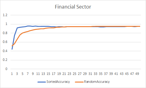
(a) Financial Sector

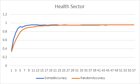
(b) Health Sector

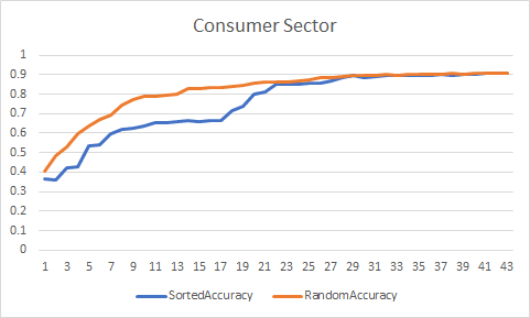
(c) Health Sector

Figure 6.8: Feature Number in Balance Sheet Coarse Mapping for Algorithm 2

From table 6.5, table 6.6, Algorithm 2 needed lesser number of feature in comparison to Algorithm 1 for most of data sets to achieve almost the same accuracy that reduced significantly the time spent on data analyzing and improved computational efficiency. In addition, the accuracy of Financial Ratio feature sets was always higher than that of Balance Sheet feature sets. From table 6.7, table 6.8, random order data sets need more number of features compared with sorted feature sets. This confirmed sorting feature sets before feature selecting was necessary that improved significantly computational efficiency.

7 Feature Classification

Factor Analysis can deal with data sets where there are a large number of observed variables that are thought to reflect a smaller number of latent variables. There are a large number of features that influence the credit rating change,Factor analysis can help to summarize similar features together to find out the latent factors that create a commonality and explain one public factor. In this Algorithm, we can reduce significantly the number of variables and obtain main factors that have effect on credit rating change to make people understand the reason of credit rating change better.

The KMO value of Energy Sector in Balance sheet was 0.5 (less than 0.6)that indicated it was not adequate for Factor Analysis.Therefore, we do not perform Factor Analysis for Energy Sector in Balance Sheet. According to four data set for four sectors, we summarized the main factors that influenced the credit rating and displayed the results by summarizing the factors of Financial Ratio and Balance Sheet for four sectors.

7.1 Financial Ratio

In this section, we summarized the Common factors in Financial Ratio for four sectors. There are seven factors that have influence on credit rating, Debt/Asset and Debt/capital Factor, Earning and Profit Factor, Cash Turnover Factor, Liquidity Factor, Stocks Value Factor, Financing Factor, Enterprise Value Factor.

7.1.1 Financial Ratio Factor 1

The first factor is Debt/Asset and Debt/capital Factor. This factor includes Long-term Debt/Invested Capital, Total Debt/Capital, Total Debt/
Total Assets, Total Debt/Total Assets 1, Long-termDebt/Book Equity, Long-term Debt/Total Liabilities, Total Debt/Equity.

The Debt to Asset ratio indicates the company’s financial leverage and tells people the percentage of the company ’s asset financed by debt, rather than equity.The higher the ratio, the higher the degree of leverage and financial risk. The ratio can be used for investors to evaluate whether the company is reliable to meet its current debt obligation and pay a return on their investment. The debt to capital ratio gives analysts and investors a better understanding of the company’s financial structure and whether the company is worth investing. Therefore, the higher the Debt/Asset and Debt/capital,the lower the credit rating.

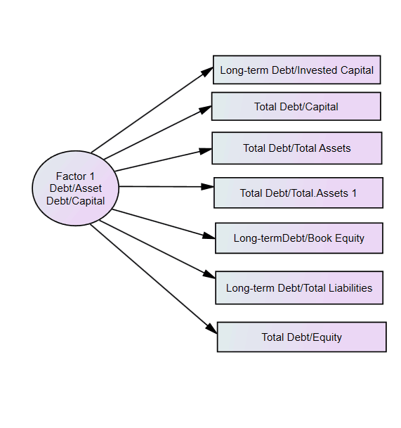
Figure 7.1: Financial Ratio: Factor 1

7.1.2 Financial Ratio Factor 2

The second factor is Earning and Profit Factor. This factor includes Pre-tax Return on Total Earning Assets, Return on Capital Employed, After-tax Return on Average Common Equity, Return on Equity, Return on Assets, After-tax Return on Invested Capital, Operating Profit Margin After Depreciation, Net Profit Margin, Gross Profit /Total Assets, Profit /Before Depreciation Current Liabilities, Operating Profit Margin Before Depreciation.

Rerurns are the earnings acquired before the interest is paid. Profit mainly included the gross profit margin, operating profit margin, and net profit margin. Profit is the money that company paid for all expense in production , sales ,taxes and so on. They are the indicator whether the company has enough funds to meet its current debt obligations and can run well in the long-run.

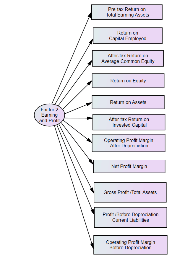
Figure 7.2: Financial Ratio Factor 2

7.1.3 Financial Ratio Factor 3

The third factor is Cash Turnover Factor. This factor includes Asset Turnover, Receivables Turnover, Inventory /Current.Assets, Payables /
Turnover. Turnover is an accounting concept that calculates the speed at which a company operates. Turnover ratio calculates the speed at which a company collects cash from accounts receivable and inventory investments. Analysts and investors use these ratios to determine whether the company is seen as a good investment.

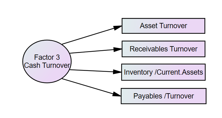
Figure 7.3: Financial Ratio Factor 3

7.1.4 Financial Ratio Factor 4

This factor is Liquidity Factor. This factor includes Cash Ratio, Cash Balance/Total Liabilities,Quick Ratio (Acid Test), Current Ratio. The cash ratio is a measure of company liquidity, especially the ratio of company cash and cash equivalents to its current liabilities.The cash ratio is a liquidity indicator of the ability of companies to use only cash and cash equivalents to cover their short-term debt.

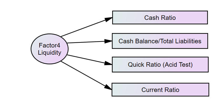
Figure 7.4: Financial Ratio: Factor 4

7.1.5 Financial Ratio Factor 5

This factor is Stocks Value Factor. This factor includes P/E(Diluted,Excl,EI), P/E(Diluted,Incl,EI). The P / E ratio is the valuation ratio of its current share price relative to its earnings per share.Investors and analysts use the P / E ratio to determine the relative value of the company’s shares for comparison with the company.

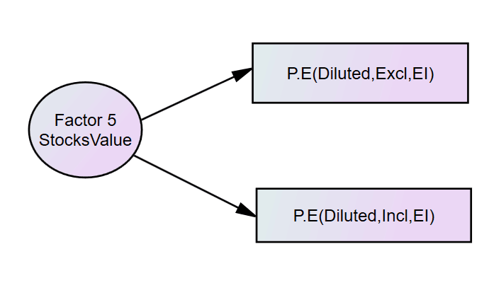
Figure 7.5: Financial Ratio Factor 5

7.1.6 Financial Ratio Factor 6

This factor is Financing Factor. This factor includes Short-Term Debt/Total Debt, Long-term Debt/ Total Liabilities, Current Liabilities /Total Liabilities. Total liabilities are the sum of individual or company debts.They are generally divided into three categories: short-term liabilities, long-term liabilities and other liabilities.Short-Term Debt/Total Debt indicates the extent of a company’s reliance on short-term financing.Long-term Debt/ Total Liabilities shows the degree of a company’s reliance on long-term financing.The larger the proportion of debt, the higher the financial leverage of the company, the less stable the company has its own capital, and the need to consider paying off the debt at any time, which will require higher cash flow of the company, so that the operating risk of the company will increase.

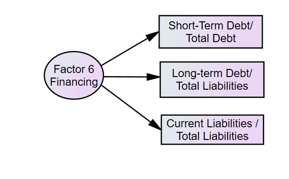
Figure 7.6: Financial Ratio Factor 6

7.1.7 Financial Ratio Factor 7

This factor is Enterprise Value Factor. This factor includes Enterprise Value Multiple, Total Debt /EBITDA. Enterprise multiple is a ratio used to evaluate the value of a company. Enterprise multiples are calculated by EBITDA according to the value of the enterprise. EBITDA is an abbreviation for earnings before interest, tax, depreciation and amortization. Enterprise multiples is used to determine whether a company is undervalue or overvalue for investors.The lower ratio, the company is more likely to be undervalue.The higher ratio, the company is more likely to be overvalue.

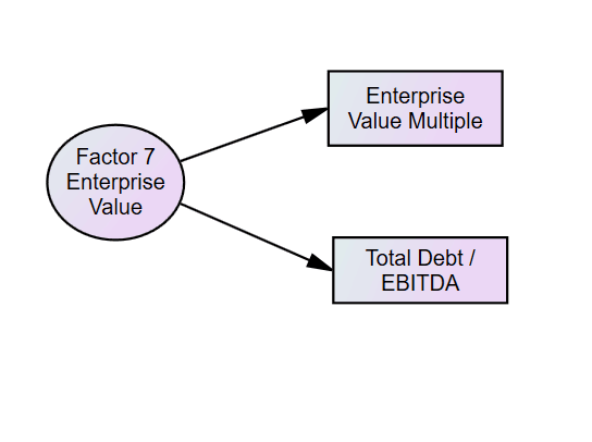
Figure 7.7: Financial Ratio Factor 7

7.2 Balance Sheet

In this section, we summarized the Common factors in Balance Sheet for four sectors. There are ten factors influencing the credit rating, Asset and liabilitied Factor, Income Factor, Implied Option Factor, Post Retirement Adjustment Factor, Pension Adjustment Factor, Earing Per Share Factor, Discontinued Operations Factor, Preferred Divifends Factor, Non-Controlling Interests Factor, and In Process R$\&$D Factor.

7.2.1 Balance Sheet Factor 1

The first factor is Asset and Liabilities Factor. This factor includes Current Assets -Other - Total, Current Liabilities -Other - Total. Current assets can reflect the operation of the company that they can be used to support daily business operation and to pay for operating expenses.The current liabilities refer to the debts or liabilities that the Company has due within one year or within the normal operating period. In addition, current liabilities are settled through the use of current assets, such as cash.Therefore, this factor represent the state of operation for a company.

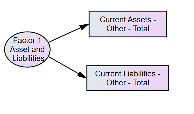
Figure 7.8: Balance Sheet Factor 1

7.2.2 Balance Sheet Factor 2

The second factor is Income Factor. This factor includes Comp Inc - Beginning Net Income, Pretax Income, Comprehensive Income-Parent, Special Items, Income Before Extra Items -Adj for Common Stock Equivalents - 12MM.Income is the company’s remaining revenues after paying all opeating expenses and taxes.The higher the income, the probably better operating state.

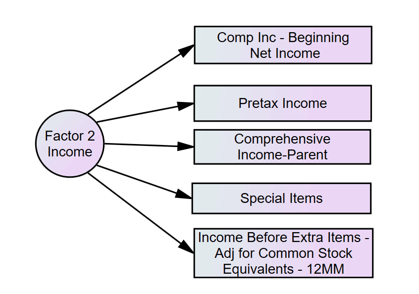
Figure 7.9: Balance Sheet Factor 2

7.2.3 Balance Sheet Factor 3

The third factor is Implied Option Factor. This factor includes Implied Option EPS Diluted, Implied Option EPS Diluted Preliminary, Implied Option EPS Diluted 12MM, Implied Option Expense, Implied Option Expense Preliminary, Implied Option Expense - 12mm. The implied option mainly refers to the pre-redemption option, which is the risk of the interest rate that the borrower can repay the risk in advance.The existence of implied options is one of the important reasons for financial risk.

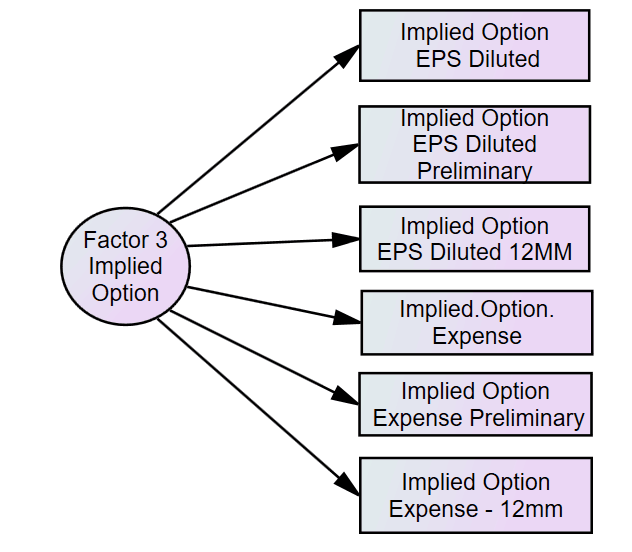
Figure 7.10: Balance Sheet Factor 3

7.2.4 Balance Sheet Factor 4

The third factor is Post Retirement Adjustment Factor. This factor includes Core Post Retirement Adjustment, Core Post Retirement Adjustment 12MM, Core Post Retirement Adjustment Diluted EPS Effect 12MM, Core Post Retirement Adjustment Diluted EPS Effect, Core Post Retirement Adjustment 12MM Diluted EPS Effect Preliminary.Retirement Adjustment will have effect on employees, which will influence operating of the company.

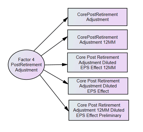
Figure 7.11: Balance Sheet Factor 4

7.2.5 Balance Sheet Factor 5

This factor is Pension Adjustment Factor.This factor includes Core Pension Interest Adjustment After-tax Preliminary, Core Pension Adjustment Preliminary, Core Pension Adjustment, Core Pension Adjustment Diluted EPS Effect 12MM, Core Pension Adjustment Diluted EPS Effect.The Pension Adjustment is a combination of all employee and employer pension credits for the year. The higher pension, the company have more funds to operate.

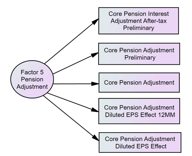
Figure 7.12: Balance Sheet Factor 5

7.2.6 Balance Sheet Factor 6

This factor is Earnings Per Share Factor.This factor includes Earnings Per Share (Diluted)-Excluding Extraordinary Items- 12 Months Moving, Earnings Per Share (Diluted)-Including Extraordinary Items.1, Core Pension w/o Interest Adjustment Diluted EPS Effect Preliminary. Earnings Per Share is the share of the company’s profits divided by its common stock. It indicates the profitability of a company. The higher the Earnings Per Share , the more profit a company obtains.

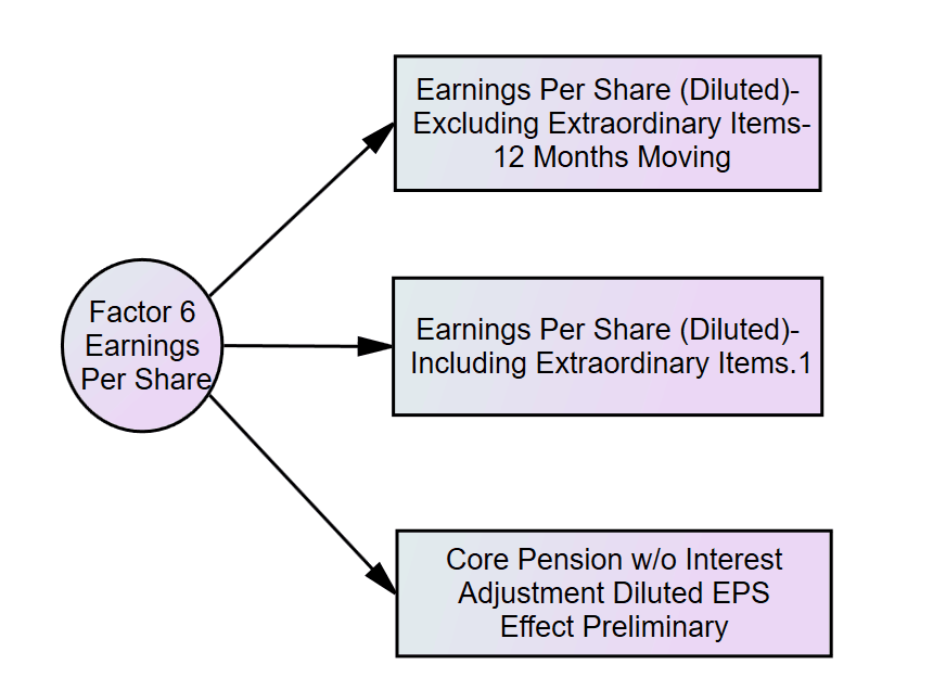
Figure 7.13: Balance Sheet Factor 6

7.2.7 Balance Sheet Factor 7

This factor is Discontinued Operations Factor. This factor includes Discontinued Operations, Extraordinary Items and Discontinued Operations
Discontinued operations is shown separately in the income statement, and investors can clearly know the profits and cash flows from the discontinued activities, especially when the company is merged, and it is better to analyze which assets are stripped or folded to understand how a company will make money in the future.

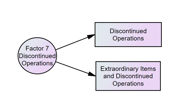
Figure 7.14: Balance Sheet Factor 7

7.2.8 Balance Sheet Factor 8

This factor is Preferred Dividends Factor. This factor includes Nonred Pfd Shares Outs (000) - Quarterly, Preferred/Preference Stock (Capital)-Total, Dividends-Preferred/Preference.A preferred dividend refers to the dividends accrued and paid by the company’s preferred shares.The higher the company’s earnings per share, the higher its profitability.

Figure 7.15: Balance Sheet Factor 8

7.2.9 Balance Sheet Factor 9

This factor is Non-Controlling Interests Factor. This factor includes Non-Controlling Interest - Redeemable - Balance Sheet, Non-Controlling Interests - Total - Balance Sheet. Non-Controlling Interests is not owned by the parent company, which owns a controlling stake (more than 50 per cent but less than 100 per cent) and merges the financial performance of the subsidiary into its own company.For investors, it is important for companies to provide transparency of non-controlled benefits, because this will enable them to better understand the impact of non-controlled benefits on the financial position, financial performance and cash flow of the company, and thus also understand the risks the company faced.

Figure 7.16: Balance Sheet Factor 9

7.2.10 Balance Sheet Factor 10

This factor is In Process R&D Factor. This factor includes In Process R&D, In Process R&D Expense After-tax.A company typically generates research and development costs as it seeks and creates new products or services.It is important for the company to maintain the forefront of innovation and invest heavily in product research and development. With the development of technology, these efforts enable the company to diversify and find new growth opportunities.

Figure 7.17: Balance Sheet Factor 10

8 Conclusion

In this paper, we selected the important features that had a significant impact on the corporate credit via Principle Component Analysis and Factor Analysis, and compared which one can better select the essential features to explain the reason for credit rating change. We optimized the sorting method of principal component analysis and factor analysis. For Principle Component Analysis, we added the the squares of loadings of every component of each feature instead of adding absolute values to avoid the influence of extreme values. As for Factor Analysis, according to the principle of the first factor priority, we sorted each factor’s features per the absolute value of loadings within the first factor and then the second factor and downwards. Then, the results showed that Factors Analysis required fewer features compared to the Principal Component Analysis to actuate the same accuracy of above 95%. Finally, we concluded dominant factors on credit rating, in the data set of Financial Ration, seven factors influencing the corporate: Debt/Asset and Debt/capital Factor, Earningand Profit Factor, Cash Turnover Factor, Liquidity Factor, Stocks Value Factor, Financing Factor,Enterprise Value Factor; in Balance Sheet, ten factors affecting the credit rating: Asset and liabilitied Factor, Income Factor, Implied Option Factor, Post Retirement Adjustment Factor, Pension Adjustment Factor, Earing Per Share Factor, Discontinued Operations Factor, Preferred Divifends Factor, Non-Controlling Interests Factor, and In Process R$\&$D Factor.

Appendix A A Top 10 features selected by Algorithm 1

A.1 Financial Sector

A.1.1 Financial Sector:Data1: Financial Ratio + Detailed Mapping

Receivables Turnover
Total Debt/Equity
Payables Turnover
Capitalization Ratio
Operating Profit Margin After Depreciation
Total Debt/Total Assets 1
Long-term Debt/Invested Capital
Research and Development/Sales
Total Liabilities/Total Tangible.Assets
Book/Market

A.1.2 Financial Sector:Data2:Balance Sheet + Detailed Mapping

Noncontrolling Interest - Redeemable - Balance Sheet
Deferred Taxes and Investment Tax Credit
Common Shares Used to Calculate Earnings Per Share - 12 Months Moving
Cost of Goods Sold
Accounting Changes - Cumulative Effect
Stock Compensation Expense
Preferred ESOP Obligation - Non-Redeemable
Property Plant and Equipment - Total (Net)
Core Pension Adjustment Diluted EPS Effect
Extraordinary Items

A.1.3 Financial Sector:Data3 :Financial Ratio + Coarse Mapping

Receivables Turnover
Total Debt/Equity
Long-term Debt/Invested Capital
Research and Development/Sales
Capitalization Ratio
Payables Turnover
P/E (Diluted, Excl. EI)
Short-Term Debt/Total Debt
Total Debt/Total Assets.1
Total Debt/Capital

A.1.4 Financial Sector:Data 4 :Balance Sheet + Coarse Mapping

Core Post Retirement Adjustment Diluted EPS Effect 12MM
Interest and Related Expense-Total
Implied Option EPS Diluted Preliminary
Preferred ESOP Obligation-Non.Redeemable
Implied Option Expense Preliminary
Pretax Income
Implied Option EPS Diluted
Current Assets-Other-Total
Cash and Short Term Investments
Carrying Value

A.2 Energy Sector

A.2.1 Energy Sector :Data1: Financial Ratio + Detailed Mapping

Price/Cash flow
Receivables Turnover
P.E(Diluted,Excl,EI)
Research and Development/Sales
Avertising Expenses/Sales
Cash Flow Margin
Total Liabilities /Total Tangible Assets
Dividend Payout Ratio
Short-Term Debt/Total Debt
Common Equity/Invested Capital

A.2.2 Energy Sector :Data2:Balance Sheet + Detailed Mapping

Non-Operating Income (Expense) - Total
Other.Long.term.Assets
Gain Loss on Sale-Core Earnings Adjusted After-tax 12MM
Non-Current Assets-Total
Comp Inc-Derivative Gains Losses
Derivative Liabilities Long-Term
Pension Core Adjustment-12mm
Goodwill(net)
Current Assets-Other-Total
Income Before Extra-Items-Adjfor Common Stock Equivalents-12MM

A.2.3 Energy Sector : Data3 :Financial Ratio + Coarse Mapping

P/E (Diluted, Excl, EI)
Book/Market
Operating.CF.Current.Liabilities
P/E (Diluted, Incl. EI)
Short-Term Debt/Total Debt
Price/Book
Return.on.Assets
Return.on.Equity
Net Profit Margin
Inventory/Current Assets

A.2.4 Energy Sector :Data 4 :Balance Sheet + Coarse Mapping

Core Post Retirement Adjustment 12MM Diluted EPS Effect Preliminary
Interest and Related Expense-Total
Implied Option EPS Diluted Preliminary
Preferred ESOP Obligation-Non Redeemable
 Implied Option Expense Preliminary
Pretax Income
Implied Option EPS Diluted
Current Assets-Other-Total
Cash and Short-Term Investments
Carrying Value

A.3 Health Sector

A.3.1 Health Sector :Data1: Financial Ratio + Detailed Mapping

Pre-tax Return on Total Earning Assets
Free Cash Flow Operating Cash Flow
After-tax Return on Average Common Equity
Inventory/Current Assets
Common Equity /Invested Capital
Operating CF/CurrentLiabilities
Sales/Stockholders Equity Sales/Working Capital
Price/Sales
ReturnonAssets

A.3.2 Health Sector :Data2:Balance Sheet + Detailed Mapping

Core Post Retirement Adjustment 12MM Diluted EPS Effect Preliminary
In Process RD Expense Aftertax
Core Post Retirement Adjustment Diluted EPS Effect 12MM
Debtin Current Liabilities
Current Liabilities-Other-Total
Earnings PerShare(Diluted)-Excluding Extraordinary items
SPCore Earnings EPS Diluted Preliminary
Interestand Related Expense Total
Total Long-term Investments
Core Post Retirement Adjustment Preliminary

A.3.3 Health Sector : Data3 :Financial Ratio + Coarse Mapping

P/E (Diluted, Excl, EI) Cash Flow/Total Debt
PretaxreturnonNet/OperatingAssets
GrossProfit/TotalAssets
CashBalance/TotalLiabilities
TotalDebt/TotalAssets
Effective Tax Rate
ProfitBeforeDepreciation/CurrentLiabilities
Price/Book
Total Liabilities/Total Tangible Assets

A.3.4 Health Sector :Data 4 :Balance Sheet + Coarse Mapping

Preferred ESOP Obligation - Non-Redeemable
In Process R&D Expense After-tax
Depreciation, Depletion and Amortization (Accumulated)
Treasury Stock - Total (All Capital)
Non-controlling Interests - Total- Balance Sheet
Non-Current Assets - Total
Core Post Retirement Adjustment Diluted EPS Effect 12MM
Core Post Retirement Adjustment 12MM Diluted EPS Effect Preliminary
Implied Option Expense
Core Post Retirement Adjustment Preliminary

A.4 Consumer Sector

A.4.1 Consumer Sector :Data1: Financial Ratio + Detailed Mapping

P/E (Diluted,Incl,EI) Common.Equity/Invested.Capital Long.term.Debt/Invested.Capital Pre-tax.Return on Total Earning Assets Net Profit Margin Gross Profit Margin Effective Tax Rate Current Liabilities/Total Liabilities Total Debt/Total Assets Profit Before Depreciation/Current Liabilities

A.4.2 Consumer Sector :Data2:Balance Sheet + Detailed Mapping

Operating Income Before Depreciation-Quarterly
Non Operating Income(Expense)-Total
Core Pension Adjustment
Core Post Retirement Adjustment 12MM Diluted EPS Effect Preliminary
Common Shares Used to Calculate Earnings Per Share - 12 Months Moving
Dilution Adjustment
Accum Other Comp Inc - Derivatives Unrealized Gain/Loss
Core Post Retirement Adjustment Preliminary
Accounting Changes-Cumulative Effect

A.4.3 Consumer Sector : Data3 :Financial Ratio + Coarse Mapping

Trailing P/E to Growth (PEG) ratio
Common Equity/Invested Capital
Pre-tax Return on Total Earning Assets
Return on Assets
Gross Profit Margin
Long-term Debt/Invested Capital
Net Profit Margin
Effective Tax Rate
Long-term Debt/Total Liabilities
Short Term Debt/Total Debt

A.4.4 Consumer Sector :Data 4 :Balance Sheet + Coarse Mapping

Operating.Income.Before.Depreciation-Quarterly
Non-Operating Income(Expense)-Total
Core Pension Adjustment
Core Post Retirement Adjustment 12MM Diluted EPS Effect Preliminary
Common Shares Used to Calculate Earnings Per Share-12.Months.Moving
Dilution Adjustment
Accum Other Comp Inc - Derivatives Unrealized Gain/Loss
Core Post Retirement Adjustment.Preliminary
Accounting Changes-Cumulative.Effect

Appendix B B Top 10 features selected by Algorithm 2

B.1 Financial Sector

B.1.1 Financial Sector:Data1: Financial Ratio + Detailed Mapping

Total Debt/Total.Assets
Total Debt/EBITDA
Long -term.Debt/Total Liabilities
Cash Flow/Total.Debt
Long-term Debt/Book Equity
Total Debt/Capital
Total Debt/Equity
Asset Turnover
Receivables Turnover
Payables Turnover

B.1.2 Financial Sector:Data2:Balance Sheet + Detailed Mapping

Account Payable Creditors-Trade
Long-Term Debt-Total
Capital Surplus Share Premium Reserve
Cash and Short-Term Investments
Goodwill(net)
Non-Operating Income (Expense) - Total
Common Shares Used to Calculate Earnings Per Share - 12 Months Moving
Preferred/Preference Stock - Nonredeemable
Sales Turnover (Net)
Depreciation and Amortization-Total

B.1.3 Financial Sector:Data3 :Financial Ratio + Coarse Mapping

Total Debt /Total Assets 1
Asset Turnover
Return on Assets
Total Debt/Equity
Cash Flow/Total.Debt
Long-term Debt/Total Liabilities
Total Debt/Capital
Receivables Turnover
Gross.Profit/Total Assets
Capitalization Ratio

B.1.4 Financial Sector:Data 4 :Balance Sheet + Coarse Mapping

Account Payable/Creditors-Trade
Long-Term Debt-Total
Capital Surplus/Share Premium Reserve
Cash and Short-Term Investments
Goodwill(net)
Non-Operating Income (Expense)-Total
Common Shares Used to Calculate Earnings Per Share-12 Months Moving
Sales Turnover (Net)
Depreciation and Amortization -Total
Retained Earnings

B.2 Energy Sector

B.2.1 Energy Sector :Data1: Financial Ratio + Detailed Mapping

Pre-tax Return on Total Earning Assets
Return on Capital Employed
After-tax Return on Average Common Equity
Return on Equity
Return on Assets
After-tax Return on Invested Capital
Operating Profit.Margin.After.Depreciation
Net Profit Margin
Gross Profit/Total Assets
Profit Before Depreciation/Current Liabilities

B.2.2 Energy Sector : Data3 :Financial Ratio + Coarse Mapping

Pre-tax Return on Total Earning Assets
Return on Capital Employed
After-tax Return on Average Common Equity
Return on Equity
Return on Assets
After-tax Return on Invested Capital
Operating Profit Margin After Depreciation
Net Profit Margin
Gross Profit/Total Assets
Profit Before Depreciation /Current iabilities

B.3 Health Sector

B.3.1 Health Sector :Data1: Financial Ratio + Detailed Mapping

Long-term Debt/Invested Capital
Common Equity/Invested Capital
Total Debt/Invested Capital
Total Debt/Total Assets
Total Debt/Capital
Long-term Debt/Book Equity
Total Debt/Total Assets1
Long-term Debt/Total Liabilities
Return on Equity
After-tax Return onI nvested Capital

B.3.2 Health Sector :Data2:Balance Sheet + Detailed Mapping

Core Post Retirement Adjustment 12MM Diluted EPS Effect Preliminary
In Process R&D Expense After-tax
Core Post Retirement Adjustment Diluted EPS Effect 12MM
Debtin Current Liabilities
Current Liabilities-Other-Total
Earnings Per Share(Diluted)-Excluding Extraordinaryitems
SP Core Earnings EPS Diluted Preliminary
Interestand Related Expense Total
Total Long-term Investments
Core Post Retirement Adjustment Preliminary

B.3.3 Health Sector : Data3 :Financial Ratio + Coarse Mapping

Long-term Debt/Invested Capital
Total Debt/Invested Capital
Common EquityInvested Capital
Total Debt/Total Assets
Total Debt/Capital
Long-term Debt Book Equity
TotalDebt/Total Assets1
Long-termDebt/Total Liabilities
Return on Equity
After-tax Return on Invested Capital

B.3.4 Health Sector :Data 4 :Balance Sheet + Coarse Mapping

Non-Current Assets-Total
Current Liabilities-Other-Total
Long-Term Liabilities-Total
Current Assets-Total
Depreciation and Amortization-Total
Operating Income After Depreciation Quarterly
Common Shares Used to Calculate Earnings Per Share-12 Months Moving
Current Assets-Other-Total
Property Plant and Equipment-Total(Net)
Research and Development Expense

B.4 Consumer Sector

B.4.1 Consumer Sector :Data1: Financial Ratio + Detailed Mapping

Pre-tax Return on Total Earning Assets
Return on Assets
Profit Before Depreciation Current Liabilities
Accruals Average Assets
Return on Capital Employed
Total Debt/Total Assets
Total Debt/Total Assets 1
Total.Debt/Capital
Cash Ratio
Quick Ratio(Acid)Test

B.4.2 Consumer Sector :Data2:Balance Sheet + Detailed Mapping

Interest and Related Expense-Total
Cost of Goods Sold
Depreciation and Amortization-Total
Long-Term Debt-Total
Property Plant and Equipment - Total (Net)
Operating Income Before Depreciation-Quarterly
Liabilities-Other
Current Liabilities-Other-Total
Operating Income After Depreciation-Quarterly
Assets - Other - Total

B.4.3 Consumer Sector : Data3 :Financial Ratio + Coarse Mapping

Pre-tax Return on Total Earning Assets
Return on Assets
Profit Before Depreciation Current Liabilities
Accruals Average Assets
Return on Capital/Employed
Total Debt/Total Assets
Total Debt/Total Assets 1
Total Debt/Capital
Cash Ratio
Quick Ratio(Acid)Test

B.4.4 Consumer Sector :Data 4 :Balance Sheet + Coarse Mapping

Special Items
Pretax Income
Comp Inc(Beginning)Net Income
Redeem Pfd Shares Outs (000)
Earnings Per Share(Diluted)-Including Extraordinary Items 1
Earnings Per Share(Diluted)from Operations
Income Before Extra Items-Adj for Common Stock Equivalents-12MM
Pension Core Adjustment-12mm
Core Pension Adjustment Diluted EPS Effect 12MM
Core Pension Adjustment Preliminary

References

- [1] Sohn, So Young, Dong Ha Kim, and Jin Hee Yoon. ”Technology credit scoring model with fuzzy logistic regression.” Applied Soft Computing 43 (2016): 150-158.
- [2] Wiginton, John C. ”A note on the comparison of logit and discriminant models of consumer credit behavior.” Journal of Financial and Quantitative Analysis (1980): 757-770.
- [3] Stefanescu, Catalina, Radu Tunaru, and Stuart Turnbull. ”The credit rating process and estimation of transition probabilities: A Bayesian approach.” Journal of Empirical Finance 16.2 (2009): 216-234.
- [4] Golbayani, Parisa, Ionuţ Florescu, and Rupak Chatterjee. ”A comparative study of forecasting corporate credit ratings using neural networks, support vector machines, and decision trees.” The North American Journal of Economics and Finance 54 (2020): 101251.
- [5] Saitoh, Fumiaki. ”Predictive modeling of corporate credit ratings using a semi-supervised random forest regression.” 2016 IEEE International Conference on Industrial Engineering and Engineering Management (IEEM). IEEE, 2016.
- [6] Angelini, Eliana, Giacomo di Tollo, and Andrea Roli. ”A neural network approach for credit risk evaluation.” The quarterly review of economics and finance 48.4 (2008): 733-755.
- [7] Tsai, Chih-Fong, and Ming-Lun Chen. ”Credit rating by hybrid machine learning techniques.” Applied soft computing 10.2 (2010): 374-380.
- [8] Oricchio, Gianluca, et al. ”SME Credit Rating Models: A New Approach.” SME Funding. Palgrave Macmillan, London, 2017. 139-171.
- [9] Petropoulos, Anastasios, Sotirios P. Chatzis, and Stylianos Xanthopoulos. ”A novel corporate credit rating system based on Student’st hidden Markov models.” Expert Systems with Applications 53 (2016): 87-105.
- [10] Abiyev, Rahib H. ”Credit rating using type-2 fuzzy neural networks.” Mathematical Problems in Engineering 2014 (2014).
- [11] Arora, Nisha, and Pankaj Deep Kaur. ”A Bolasso based consistent feature selection enabled random forest classification algorithm: An application to credit risk assessment.” Applied Soft Computing 86 (2020): 105936.
- [12] Yeh, Ching-Chiang, Fengyi Lin, and Chih-Yu Hsu. ”A hybrid KMV model, random forests and rough set theory approach for credit rating.” Knowledge-Based Systems 33 (2012): 166-172.
- [13] Jiang, Hao, et al. ”Stationary Mahalanobis kernel SVM for credit risk evaluation.” Applied Soft Computing 71 (2018): 407-417.
- [14] İç Y T. A multi-objective credit evaluation model using MOORA method and goal programming[J]. Arabian Journal for Science and Engineering, 2019: 1-14.
- [15] Addo P M, Guegan D, Hassani B. Credit risk analysis using machine and deep learning models[J]. Risks, 2018, 6(2): 38.
- [16] Nehrebecka N. Predicting the default risk of companies. Comparison of credit scoring models: LOGIT vs Support Vector Machines[J]. Econometrics, 2018, 22(2): 54-73.
- [17] Angilella S, Mazzù S. The financing of innovative SMEs: A multicriteria credit rating model[J]. European Journal of Operational Research, 2015, 244(2): 540-554.
- [18] Hajek P, Michalak K. Feature selection in corporate credit rating prediction[J]. Knowledge-Based Systems, 2013, 51: 72-84.
- [19] Golbayani, Parisa, Dan Wang, and Ionut Florescu. ”Application of Deep Neural Networks to assess corporate Credit Rating.” arXiv preprint arXiv:2003.02334 (2020).
- [20] Zhou, Yimin, et al. ”A moment-based criterion for determining the number of components in a normal mixture model.” Journal of Systems Engineering and Electronics 28.4 (2017): 801-809.
- [21] Wang, Dan, Tianrui Wang, and Ionuţ Florescu. ”Is Image Encoding Beneficial for Deep Learning in Finance? An Analysis of Image Encoding Methods for the Application of Convolutional Neural Networks in Finance.” arXiv preprint arXiv:2010.08698 (2020).