Global View of Axion Stars with (Nearly) Planck-Scale Decay Constants

Abstract

We show that axion stars formed from axions with nearly Planck-scale decay constants $f$ are unstable to decay, and are unlikely to have phenomenological consequences. More generally, we show how results at smaller $f$ cannot be naively extrapolated to $f={\mathcal{O}}(M_{P})$ as, contrary to conventional wisdom, gravity and special relativity can both become relevant in the same regime. We clarify the rate of decay by reviewing and extending previous work on oscillons and axion stars, which imply a fast decay rate even for so-called dilute states at large $f$.

I Introduction

Axions Peccei and Quinn (1977a, b); Weinberg (1978); Wilczek (1978); Dine et al. (1981); Zhitnitsky (1980); Kim (1979); Shifman et al. (1980) and axion-like particles (ALPs) Turner (1983); Press et al. (1990); Sin (1994); Hu et al. (2000); Goodman (2000); Peebles (2000); Amendola and Barbieri (2006); Li et al. (2014); Marsh (2016); Hui et al. (2017); Lee (2018) originate in numerous physical theories of physics beyond the Standard Model. Their low-energy phenomenology is governed by two energy scales: the particle mass $m$ and the decay constant $f$. If the axions are pseudo-Goldstone bosons, they can be described by a periodic potential that respects an approximate shift symmetry on the axion field $\phi$, commonly taking the form

$$V(\phi)=m^{2}f^{2}\,\left[1-\cos\left(\frac{\phi}{f}\right)\right].$$ (1)

The leading self-interaction term in the expansion of $V(\phi)$ at $\phi\ll f$ gives rise to a $\lambda_{4}\phi^{4}$ potential with attractive coupling $\lambda_{4}=-m^{2}/f^{2}$; higher-order self-interaction terms become relevant at high densities Eby et al. (2016a); Visinelli et al. (2018). Such fields might be probed by current and near-future experiments, even if they possess only gravitational couplings to ordinary matter Grin et al. (2019).

Light scalars (like axions and ALPs) can constitute dark matter (DM) in the universe Preskill et al. (1983); Abbott and Sikivie (1983); Dine and Fischler (1983), and field overdensities can collapse to form bound states known as boson stars (here, axion stars); these are held together through a balance of kinetic pressure, gravitational attraction, and self-interactions Kaup (1968); Ruffini and Bonazzola (1969); Breit et al. (1984); Colpi et al. (1986); Seidel and Suen (1990); Friedberg et al. (1987); Seidel and Suen (1991); Liddle and Madsen (1992); Lee and Pang (1992); Chavanis (2011); Chavanis and Delfini (2011); Eby et al. (2016a). The standard lore is that axion stars are solutions of the equations of motion falling into three distinct classes of increasing density, known respectively as the dilute, transition, and dense branches of solutions, each with distinct macroscopic properties and stability constraints (see for example Visinelli et al. (2018); Braaten and Zhang (2019); Zhang (2019); Eby et al. (2019)).

Axion stars on the dilute branch are generally stable both under perturbations Chavanis (2011); Chavanis and Delfini (2011) and to decay Eby et al. (2016b, 2018a). Recently both simulations Schive et al. (2014a); Levkov et al. (2018); Eggemeier and Niemeyer (2019) and analytic arguments Kirkpatrick et al. (2020) have suggested that they can efficiently form in the early universe; as such, dilute axion stars have been investigated for possible phenomenological effects, including recent analyses of radio photon emission Hertzberg and Schiappacasse (2018); Hertzberg et al. (2020a); Levkov et al. (2020); Amin and Mou (2020) and gravitational lensing Croon et al. (2020a); Prabhu (2020); Croon et al. (2020b). For the attractive $\phi^{4}$ potential, there is a maximum stable mass of order $M_{P}/\sqrt{|\lambda_{4}|}=M_{P}\,f/m$ (for $\lambda_{4}=-m^{2}/f^{2}<0$, and with $M_{P}=1.22\times 10^{19}$ GeV) which signals a crossover to the structurally unstable transition branch Chavanis (2011); Chavanis and Delfini (2011); Eby et al. (2015); Schiappacasse and Hertzberg (2018). Because transition states are unstable to perturbations, they are unlikely to have observable consequences.

On the third branch, so-called dense axion stars have received considerable interest in recent years. The “dense” moniker was coined in Braaten et al. (2016a) when the configurations were investigated using the nonrelativistic equation of motion; note however that they are fundamentally no different from axitons, discussed decades earlier in a cosmological context by Kolb and Tkachev Kolb and Tkachev (1994). Today, dense axion stars / axitons are understood to be strongly bound with momentum dispersion of order $m$, and as a consequence, they decay to relativistic axions with a short lifetime and are unlikely to have phenomenological consequences Eby et al. (2016a); Visinelli et al. (2018).

In this work, we investigate the nature of axion stars at large $f$, approaching the Planck scale. The reader may wonder whether the case of large $f$ is well-motivated enough to warrant a full investigation; to allay this critique, we review several contexts in which this parameter space is commonly invoked:

• The QCD axion Peccei and Quinn (1977a, b); Weinberg (1978); Wilczek (1978); Dine et al. (1981); Zhitnitsky (1980); Kim (1979); Shifman et al. (1980) is motivated by its ability to solve the strong CP problem while simultaneously producing a good DM candidate. This model imposes a relation between the two relevant scales such that $m\,f\simeq 6\times 10^{-3}$ GeV² Di Vecchia and Veneziano (1980); Grilli di Cortona et al. (2016). The abundance of dark matter QCD axions depends on cosmological assumptions, with masses $m\gtrsim\mu$eV required if the global symmetry of the axion is broken after inflation, corresponding to relatively low $f\lesssim 6\times 10^{12}$ GeV (see Gorghetto et al. (2020) for a recent, more stringent bound on the post-inflationary scenario). On the other hand, if symmetry breaking occurs before inflation, then masses all the way down to $m\simeq 5\times 10^{-13}$ eV are allowed (at the expense of tuning the initial misalignment angle, see e.g. Grilli di Cortona et al. (2016), or non-minimal model-building, e.g. Bonnefoy et al. (2019)), in which case $f\simeq M_{P}$ is obtained. Even in such a model, where there are no large primordial density fluctuations, it may be possible to form axion stars through large misalignment Arvanitaki et al. (2020).

• In other particle physics models, the scales $m$ and $f$ characterizing the axion are independent. ALPs may, for example, originate from string theory at low-energy from string compactification or as a consequence of anomaly cancellation Svrcek and Witten (2006); Cicoli et al. (2012); Arvanitaki et al. (2010). In such cases the decay constant $f$ is naturally very large, of order the Grand Unified Theory (GUT) scale $\Lambda_{GUT}\simeq 10^{16}$ GeV or higher. A widely-known example is Ultralight DM (ULDM) Hu et al. (2000); Press et al. (1990); Sin (1994); Turner (1983); Peebles (2000); Amendola and Barbieri (2006); Marsh (2016); Hui et al. (2017); Lee (2018), where $m\simeq 10^{-22}-10^{-20}$ eV implies galaxy-scale axion wavelengths, and axion stars forming in the central cores of galaxies Schive et al. (2014b, a); Mocz et al. (2017); Veltmaat et al. (2020); Nori and Baldi (2020). Another well-motivated particle physics model is coherent relaxion dark matter, which may also require $f\gtrsim\Lambda_{GUT}$ in order to be consistent with constraints from fifth-force experiments Banerjee et al. (2019).

• A more phenomenologically-driven parameter choice is $f\sim M_{P}$ and $m\sim 10^{-10}$ eV, as the dilute bound states become very compact, having (at their maximum stable mass) roughly the size and mass of neutron stars: $R={\mathcal{O}}$(few) km and $M={\mathcal{O}}(M_{\odot})$. Such states may collide with other astrophysical bodies, giving rise to gravitational wave signals Clough et al. (2018); Dietrich et al. (2019).

• Axion stars have also been investigated as the origin of certain black holes in the universe. At small $f$, it is known that axion stars which grow unstable and collapse do not form black holes, as they are stabilized by a core repulsion; they instead explode in a burst of scalar radiation in their approach to the dense configuration, a process known as a Bosenova Eby et al. (2016a, 2017); Levkov et al. (2017); Helfer et al. (2017). But at large $f\gtrsim 0.1\,\tilde{M}_{P}$ (where $\tilde{M}_{P}=2.4\times 10^{18}$ GeV is the reduced Planck mass), it has been suggested that collapse can indeed lead to formation of black holes Helfer et al. (2017); Chavanis (2018); Michel and Moss (2018); Widdicombe et al. (2018). If true, this process could explain the tentative recent observation of a black hole of $M\sim 2-3M_{\odot}$ by the LIGO/VIRGO collaborations Abbott et al. (2020), which lies in a mass gap not easily explained by standard theories of black hole formation.

On the basis of this and other work, we conclude that the parameter range $\Lambda_{\rm GUT}\lesssim f\lesssim M_{P}$ is motivated, and warrants the study we put forward here.

In this work, we show that the naive picture of three branches of axion stars outlined above breaks down as the decay constant $f$ approaches $M_{P}$, due to the usual assumptions about the relevance of gravity and special relativity breaking down. This fact implies that previous naive estimations of axion star parameters in this regime have neglected important contributions. In addition, we will point out that axion stars with large $f$ become unstable to decay to relativistic particles, even on the dilute branch; as a result, such axion stars are unlikely to be phenomenologically relevant in the manner described above. We will make this point by reviewing calculations for the decay rate in previous literature, extending them to include gravity and higher-order self-interactions, and finally determining the full range of stable axion star solutions.

We will use natural units throughout, where $\hbar=c=1$.

II Axion Stars

II.1 Non-Relativistic Bound States

We first review a few relevant facts about axion stars, which are derivable using a number of viable methods Eby et al. (2019); for our purposes, the formalism of Ruffini and Bonazzola (RB) Ruffini and Bonazzola (1969) is the most useful. RB used an expansion of the axion field operator which was linear in creation and annihilation operators to describe axionic bound states when self-interactions were absent; their work was first extended to the case of an attractive $\phi^{4}$ self-interaction in Barranco and Bernal (2011). Some of the present authors further extended the analysis to fully characterize the attractive $\phi^{4}$ case Eby et al. (2015), and also to include contributions from scattering states that give rise to decay processes Eby et al. (2016b, 2018a) and relativistic corrections to bound states Eby et al. (2018b).

The generic, spherically-symmetric RB field operator can be written in the form

$$\phi(t,r) =R(r)\left[e^{-i\,\epsilon\,m\,t}\,a_{0}+h.c.\right] {\rm(RB)}$$

$$\qquad+\sum_{k>1}^{\infty}R_{k}(r)\left[e^{-i\,k\,\epsilon\,m\,t}\,a_{0}^{k}+h.c.\right] {\rm(GRB)}$$

$$\qquad+\left[\psi_{f}(t,r)+h.c.\right], {\rm(Scattering)}$$ (2)

where $R(r)$, $R_{k}(r)$, and $\psi_{f}(t,r)$ are the $N$-particle bound ground state, higher-harmonic states, and single-particle scattering state wavefunctions (respectively), $a_{0}$ and its conjugate are the annihilation and creation operators for the bound state, and $\epsilon\,m<m$ is the bound state eigenenergy. The scattering and higher-order harmonic modes were not included by RB, and will be discussed in the next sections. In the weak binding limit, where $|\epsilon-1|\ll 1$, it is appropriate to rescale the wavefunction as $Y(x)=2\sqrt{N}R(r)/(f\,\Delta)$ with the coordinate rescaled as $x=\Delta\,m\,r$ Eby et al. (2015), where $\Delta\equiv\sqrt{1-\epsilon^{2}}$.

Color	Red	Green	Brown	Purple
$\delta$	$10^{-4}$	$10^{-3}$	$10^{-2}$	$10^{-1}$
$f$ [GeV]	$2.4\times 10^{16}$	$7.7\times 10^{16}$	$2.4\times 10^{17}$	$7.7\times 10^{17}$
$f/M_{P}$	$2\times 10^{-3}$	$6.3\times 10^{-3}$	$0.02$	$0.063$
$f/\tilde{M}_{P}$	$0.01$	$0.032$	$0.1$	$0.32$
$f/\Lambda_{\rm GUT}$	$2.4$	$7.7$	$24$	$77$
$\kappa$ ($\Delta=0.1$)	$0.01$	$0.1$	$1$	$10$

Table 1: Relationship between the expansion parameter $\delta$, the decay constant $f$, and the effective gravitational coupling $\kappa$, and the corresponding color in the Figures, over the range of inputs considered in this work. Note for reference that $M_{P}=1.22\times 10^{19}$ GeV, $\tilde{M}_{P}=2.4\times 10^{18}$ GeV and $\Lambda_{\rm GUT}=10^{16}$ GeV.

Bound-state configurations can be determined by solving the coupled Einstein+Klein-Gordon (EKG) equations for the wavefunction $Y(x)$, along with the functions determining the gravitational metric. In the Newtonian and nonrelativistic limits, the equations of motion are Eby et al. (2015)

$$\nabla^{2}Y(x) =-\frac{1}{8}\,Y(x)^{3}+[1+\kappa\,b(x)]\,Y(x),$$ (3)

$$b(x) =-\frac{1}{8\pi}\left[\int d^{3}x^{\prime}\frac{Y(x^{\prime})^{2}}{|\vec{x}-\vec{x}^{\prime}|}\right],$$ (4)

where the spherically-symmetric metric function $g^{tt}=1-\delta\,b(x)$ with $\delta=8\pi\,f^{2}/M_{P}^{2}$; the other relevant metric function $g^{rr}=1-\delta\,a(x)$ was eliminated using the $rr$ Einstein equation. Note that we have taken the potential to be that of Eq. (1); it has been shown that in this case the above equations are equivalent to the Schrödinger+Poisson equations often used in the study of boson stars Eby et al. (2018c).

The set of equations (3-4) represents the leading order in a double-expansion of the relativistic EKG equations in the two small parameters $\delta\ll 1$ (representing weak, Newtonian gravity) and $\Delta\ll 1$ (representing weak binding, or the nonrelativistic limit); as written, they are correct to ${\mathcal{O}}(\delta,\Delta^{2})$ Eby et al. (2015), and in the next section we extend to the next order in special-relativistic corrections, ${\mathcal{O}}(\Delta^{4})$. Previous perturbative studies have been restricted to either the fully nonrelativistic limit (e.g. Chavanis (2011) and many others), or they include leading-order special relativity but neglect Newtonian gravity Mukaida et al. (2017); Braaten et al. (2016b); Namjoo et al. (2018); Braaten et al. (2018); in the next section, we attempt to bridge this gap by including both effects. For a detailed discussion of the relativistic expansion parameters, see Eby et al. (2019).

There exist higher-order corrections proportional to $\delta\,\Delta^{2}$ or $\delta^{2}$, which we require to be subleading by restricting the maximum parameter values $\delta_{\rm max}=0.1\ll\Delta_{\rm max}^{2}=1/2$ throughout; the effect of these subleading terms was partially investigated in Croon et al. (2019), but for simplicity we leave a full study for future work.

The one free parameter in Eqs. (3-4) is $\kappa=\delta/\Delta^{2}$, which is the effective coupling to gravity. For a given value of $\kappa$, these coupled equations have a unique solution that is easily determined by the standard shooting method: one varies the central values $Y(0)$ and $b(0)$ until there is exponential convergence $Y(x\to x_{\rm max})\to 0$ and $a(x\to x_{\rm max})+b(x\to x_{\rm max})\to 0$ at some large $x_{\rm max}$. This can be done to arbitrarily high precision (see Eby et al. (2015) for details). For clarity we translate between values of $\delta$, $f$, and $\kappa$ in Table 1 for the range we investigate here.

Eqs. (3-4) are, in most applications, sufficient to describe the dilute and transition branches of axion star solutions. On the stable dilute branch, the total mass $M\propto\Delta$ and the radius $R\propto\Delta^{-1}$, so that $M\propto R^{-1}$. Stable solutions have $\kappa\geq\kappa_{c}\equiv 0.34$; the inequality is saturated at a maximum stable mass $M_{\rm c}=10.2\,M_{P}\,f/m$, which corresponds to a critical value of

$$\Delta_{c}\approx\sqrt{\frac{8\pi}{\kappa_{c}}}\,\frac{f}{M_{P}}=8.6\,\frac{f}{M_{P}}.$$ (5)

Beyond this critical point, the central density $Y(0)$ grows while the gravitational coupling $\kappa$ continues to decrease below unity, leading to a decoupling of gravity which characterizes the transition branch.

From here we can already see that naive extrapolation to $f={\mathcal{O}}(M_{P})$ will fail, as Eq. (5) predicts $\Delta_{c}={\mathcal{O}}(1)$ or larger. In reality, we will find in the next section that above some value of $f$ this naive maximum mass point is no longer attainable. Indeed, when $\Delta$ becomes large, the eigenenergy in the axion star approaches $m$, implying a breakdown of the nonrelativistic approximation Eby et al. (2019). This also affects the bound state and leads to relativistic decay processes that render the star unstable; we discuss both effects below.

II.2 Bound States with Relativistic Corrections

There have recently been several independent efforts to quantify the effect of relativistic corrections on axion stars, which are relevant at large densities Mukaida et al. (2017); Braaten et al. (2016b); Namjoo et al. (2018); Braaten et al. (2018). In one such work, it was shown how such corrections can be organized as a power series in the parameter $\Delta$ by extending the RB framework, thereby defining a Generalized Ruffini-Bonazzola (GRB) procedure Eby et al. (2018b). In that work gravity was negligible, because (a) the focus was on the transition / dense branches of solutions, and (b) the input parameters were assumed to be in the standard range for QCD axion experiments, where $f\sim 10^{10-12}$ GeV. However at large $f$, the parameters $\delta$ and $\Delta$ can be of the same order, and therefore both Newtonian gravity and special-relativistic corrections must be taken into account.

At leading order in higher-harmonic (GRB) corrections of Eq. (II.1), Eq. (3) is modified as Eby et al. (2018b)

$$\nabla^{2}Y(x) =-\frac{1}{8}\,Y(x)^{3}+[1+\kappa\,b(x)]\,Y(x)+\frac{3}{512}\Delta^{2}\,Y(x)^{5},$$ (6)

where we continue to use the potential of Eq. (1). Once again, note that we ignore corrections proportional to $\delta\,\Delta^{2}$, which appeared in Croon et al. (2019), or proportional to $\delta^{2}$, which are post-Newtonian, because such corrections are small for the parameter space we consider.

The mass $M$ of the axion star at leading-order in GRB is $M={\mathcal{M}}(x_{\rm max}\to\infty)$ with

$${\mathcal{M}}(x_{\rm max}) =\frac{\pi\,f^{2}}{m\,\Delta}\int_{0}^{x_{\rm max}}dx\,x^{2}\Big{[}(2-\Delta^{2}+\delta\,a(x))Y(x)^{2}$$

$$\quad+\Delta^{2}\,Y^{\prime}(x)^{2}-\frac{\Delta^{2}}{16}Y(x)^{4}+\frac{\Delta^{4}}{512}Y(x)^{6}\Big{]}.$$ (7)

We define the radius as $R_{99}$, inside which $0.99$ of the mass is contained,

$${\mathcal{M}}(\Delta\,m\,R_{99})=0.99\times M.$$ (8)

To the extent that the number of particles is conserved—a topic we will return to in the next section—we can treat axion stars as $N$-particle states with $N=M/m$.

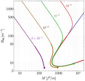
Figure 1: The mass-radius relation for axion stars at leading-order in GRB, obtained by solving Eqs. (4 , 6-8). The curves are labeled by values of $\delta$ and color-coded as in Table 1; the blue curve corresponds to the limit of gravity decoupling, $\kappa\to 0$. Configurations on the solid curves are stable to decay processes with long lifetimes $\tau_{0}>\tau_{U}$; those along the dashed curves are unstable to decay. The filled circles represent the endpoint of each curve at $\Delta=1/\sqrt{2}$.

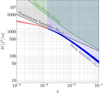
Figure 2: Critical lines of stability for axion stars in the plane of mass $M$ vs $\delta$. The black shaded region marks gravitational instability, $M>M_{\rm max}$; the green shaded region marks large binding energies $\Delta>1/\sqrt{2}$; and the blue shaded region denotes parameter space on the dilute branch of solutions with short lifetimes $\tau_{0}<\tau_{U}$. The red band denotes the crossover to decay instability on the transition branch. For both blue and red bands, the width represents the axion particle mass varied in the range $10^{-20}$ eV $\leq m\leq 1$ eV.

The system of equations (4 , 6) requires two input parameters, $\Delta$ and $\kappa$, though at fixed $\Delta$ we can trade $\kappa$ for the more intuitive parameter $\delta$. Then the solutions have masses and radii computable using Eqs. (II.2-8); the results are depicted in Fig. 1, where the curves are labeled by values of $\delta$ and color-coded as in Table 1. The blue line corresponds to $\kappa\to 0$ or full gravitational decoupling. The endpoints of each curve (marked with a filled circle) represent $\Delta=\Delta_{\rm max}=1/\sqrt{2}$, essentially an arbitrary cutoff; at $\Delta_{\rm max}$, not only does the GRB expansion break down, but the binding energy is so large that the momentum uncertainty becomes comparable to the mass $m$, and the usual methods of analysis fail Eby et al. (2019). Note for future reference that on the red curve, $f\simeq 2.4\,\Lambda_{\rm GUT}$, and on the purple curve $f\simeq 0.3\,\tilde{M}_{P}$.

For low $f\lesssim 10^{17}$ GeV, we see in Fig. 1 the standard separation into three distinct branches of solutions. The dilute and transition branches are joined at the (local) maximum mass $M_{\rm max}$, while the transition and dense branches are joined at a (local) minimum mass $M_{\rm min}\sim{\rm few}\times 100f^{2}/m$. As $f$ grows, we find at this order in $\Delta$ that the transition branch shrinks, while simultaneously the cutoff at high $\Delta$ limits the extent of the dense branch, leaving only the dilute branch intact. It is possible that between our cutoff $\Delta_{\rm max}=1/\sqrt{2}$ and the maximum possible value $\Delta=1$ that some portion of the dense branch persists; however, the transition branch is almost certainly lost, as we see the dilute and dense branches joining to a single point between $\delta=10^{-1}$ and $\delta=10^{-2}$.

In previous literature, it has always been assumed that the region where relativistic corrections are important is nonoverlapping with the region where gravity is important; usually the dense and dilute branches are separated by a large transition parameter space. However, we see in Fig. 1 that this assumption is badly violated as $f$ grows above $\Lambda_{\rm GUT}$. At $\delta=10^{-1}$ (purple curve), the high-$\Delta$ cutoff occurs very close to $M_{\rm max}$; we were unable to push to larger $\delta$ in this analysis due to the appearance of higher-order corrections, but it is plausible that for $\delta={\mathcal{O}}(1)$ the naive maximum mass is never reached. Other aspects of the solutions in Fig. 1 will be discussed in the next section.

An important consequence of Eq. (6) for large $f$ is that due to shifts in the parameter $\Delta$ as $f$ increases, decay processes can be relevant even on the dilute and transition branches. We address this in the next section.

III Decay Rate

Axion stars decay through emission of relativistic particles. There are two classes of decay modes, which proceed through tree-level Eby et al. (2016b); Mukaida et al. (2017); Eby et al. (2018a) and loop-level Braaten et al. (2017) diagrams. Importantly, the momentum distribution of bound axions has a finite width, which allows for tree-level decay processes that would be forbidden by energy-momentum conservation for particles in momentum eigenstates Eby et al. (2016b, 2018a). For a $\phi^{n}$ potential, the leading process of this type is $(n-1)\,a_{c}\to a_{f}$, where $n-1$ bound (“condensed”) axions $a_{c}$ annihilate to a single relativistic axion $a_{f}$ emitted from the star. We focus below on this tree-level decay process, though of course our conclusions would only be made stronger if higher-order processes were included as well.

In the specific case of the axion potential in Eq. (1), the leading self-interaction potential at ${\mathcal{O}}(\phi^{4})$ gives rise to a $3\,a_{c}\to a_{f}$ decay process. One can approximate the decay rate $\Gamma_{3}$ for this process by taking the matrix element of the self-interaction potential, between the initial state $\langle N\,a_{c}|$ and final state $|(N-3)\,a_{c}+1a_{f}\rangle$. The outgoing particle is emitted as a spherical wave, conserving average momentum for the [remaining condensate $+$ free particle] system (see Eby et al. (2018a) for a detailed discussion).

Previous work on relativistic decay processes in axion stars Eby et al. (2016b); Levkov et al. (2017); Visinelli et al. (2018); Eby et al. (2018a) have assumed the decoupling of gravity in the region where decay becomes relevant. However, we find in this work that gravity does not decouple in this way when $f$ becomes large, and thus we repeat the calculation of the lifetime in the Appendix A, including both effects.

A second assumption made in previous work is that the axion star can track its equilibrium configuration as it decays, which we refer to as the adiabatic approximation. However, simulation results Levkov et al. (2017); Visinelli et al. (2018), previous semi-analytic estimations Eby et al. (2016b, 2018a), as well as the present work (see Appendix A), all suggest that when decay becomes relevant, the resulting explosion of relativistic particles is extremely rapid, likely to greatly outpace the relaxation of the star back to equilibrium. Therefore in this work, we argue that an instantaneous approximation for the lifetime of axion stars is more appropriate. We thus define the lifetime as

$$\tau_{0}=\frac{N}{3}\frac{1}{\Gamma_{3}},$$ (9)

following Eq. (4.1) of Eby et al. (2016b) evaluated in the instantaneous limit. This lifetime can be uniquely determined for each configuration (on any branch of solutions), which we compare to the age of the universe $\tau_{U}\approx 13.8\times 10^{9}$ years.

As described in the Appendix A, we find that there is a sharp transition from $\tau_{0}\gg\tau_{U}$ (stability) to $\tau_{0}\ll\tau_{U}$ (instability) over a narrow range of $M$, which we define $M_{\tau}(\delta)$. In Fig. 1, we mark $M_{\tau}$ by the change from solid (stable, $\tau>\tau_{U}$) to dashed (unstable, $\tau<\tau_{U}$) lines on each curve. Importantly, at large enough $f$, the critical point $M_{\tau}$ occurs on the dilute branch, which has until now been regarded as perfectly stable.

The precise value of $M_{\tau}$ depends exponentially on $\Delta$ but only polynomially on $m$. Owing to this functional dependence, the transition from $\tau<\tau_{U}$ to $\tau>\tau_{U}$ occurs at a very sharply defined $M_{\tau}$, varying only by at most a factor of $2$ as the axion mass $m$ varies between $10^{-20}-1$ eV.

We further illustrate in Fig. 2 how the decay instability (blue shaded region) sets in on the dilute branch, at lower mass than the onset of gravitational instability (black shaded region), when $\delta\gtrsim 10^{-3}$ ($f\gtrsim 8\times 10^{16}$ GeV). The limit of very large binding energy, where $\Delta=1/\sqrt{2}$, where our approximation is no longer valid, is illustrated by the green shaded region. The blue band represents $M_{\tau}(\delta)$, and its width represents its variation upon varying $m$ in the range $10^{-20}-1$ eV. The red band similarly represents the onset of decay instability on the transition branch of solutions for smaller $\delta$.

IV Discussion

In this work, we have analyzed the structure and stability of axion stars when the decay constant $f$ is large, with a focus on the approach to the Planck scale $M_{P}$. Such scenarios are motivated by a significant body of literature, and previous work has typically assumed that results at smaller $f$ can be extrapolated to large $f$. We have shown that this extrapolation is erroneous; at the order of $\Delta$ that we consider, the dense and transition branches of solutions no longer exist above $\delta\gtrsim 10^{-1}$ ($f\gtrsim 8\times 10^{17}$ GeV) up to very large $\Delta=1/\sqrt{2}$, and the decay instability point $M_{\tau}$ occurs on the dilute branch for $\delta\gtrsim 10^{-3}$ ($f\gtrsim 8\times 10^{16}$ GeV), as shown in Fig. 1.

This result has applications in any scenario where axion stars form with $f\gtrsim 10^{17}$ GeV, including those outlined in the introduction. For example, for ULDM with particle mass $m\sim 10^{-22}$ eV, the correct relic abundance is obtained for $f\sim 10^{17}$ GeV Hui et al. (2017). ULDM simulations generally find axion stars forming the cores of galaxies in this scenario Schive et al. (2014b, a); Mocz et al. (2017); Veltmaat et al. (2020); Nori and Baldi (2020), with masses that are safely below the instability points we find here; however, if the axion star masses had been a factor of $\sim 80$ larger at formation, or if they can accrete mass efficiently, then ULDM axion stars would not merely collapse but also decay on the dilute branch, strengthening the argument of previous studies Eby et al. (2018d) (see Appendix B for details). Such an effect would not be seen in standard ULDM simulations, as they typically neglect both the self-interaction potential as well as relativistic effects. As simulations of axion star formation and accretion become more precise, or as nonminimal axion models are investigated, this must be taken into account in the final analysis.

Further, phenomenological studies of axion stars (including those looking for gravitational wave signals Clough et al. (2018); Dietrich et al. (2019) or new black hole formation mechanisms Helfer et al. (2017); Chavanis (2018); Michel and Moss (2018); Widdicombe et al. (2018)) must acknowledge that decay may make their proposed configurations unstable. For $f\simeq 7\times 10^{17}$ GeV, the mass of truly stable axion stars is already a factor of $\sim 3$ lower than the usual boundary of gravitational stability, as shown in Fig. 2. This in fact precludes axion stars with neutron star-like masses and radii by nearly an order of magnitude.

We should point out, of course, that our own results should not be naively extrapolated either. For example, in the limit $f\to\infty$ the axion self-interactions will decouple, and in that limit neither nonrelativistic collapse nor relativistic decay processes discussed here destabilize the star. Taking $f>M_{P}$ may, however, be in tension with theoretical considerations like the Weak Gravity Conjecture (see e.g. Montero et al. (2015)), though there may be ways to reconcile them Kaplan and Rattazzi (2016); Fonseca et al. (2019).

Previous works have also considered decay modes other than $3\to 1$, including so-called quantum decay (e.g. $4\to 2$) Hertzberg (2010), other classical decay processes (e.g. $5\to 1$) for alternate axion potentials Zhang et al. (2020), or for repulsive self-interactions Hertzberg et al. (2020b). In some contexts it is claimed that the resulting decay modes can actually dominate the decay rate. Because we have not included such contributions in this work, we emphasize that the lifetime we calculate is merely an upper bound on the true axion star lifetime.

We found in our study that higher-order corrections to the EKG equations appear not only at higher orders in $\Delta^{2}$ (as found in Eby et al. (2018b)), but also as powers of the product $\delta\,\Delta^{2}$ and as $\delta^{2}$; as a result we were not able to robustly analyze configurations with $\delta\gtrsim 0.1$, corresponding to $f\gtrsim 8\times 10^{17}$ GeV. We leave the effect of these corrections, and the (in)stability of axion stars with $\delta={\mathcal{O}}(1)$, for a future study, It would also be worthwhile to make a thorough comparison of our results, which apply to static axionic configurations, to the dynamical works of Helfer et al. (2017); Widdicombe et al. (2018) which use very different initial conditions; see Appendix B for a more heuristic comparison.

Note Added

After completion of this project, a related work Zhang (2020) appeared, which illustrates a different method but comes to many of the same conclusions. We believe the two papers complement one another.

Appendix A Detailed Calculation of the Decay Rate

A.1 Position of the Singularity at $\kappa\neq 0$

To analyze decay processes, in previous work some of us showed how to extend the RB field operator to include a scattering state contribution in Eq. (II.1), allowing axion quanta with energy $\omega_{p}>m$ Eby et al. (2016b, 2018a). The scattering state wavefunction $\psi_{f}$, at leading order in spherical harmonics, is given by

$$\psi_{f}(t,r)=\frac{1}{2\pi^{2}}\int_{0}^{\infty}\frac{dp\,p}{2\omega_{p}}\,j_{0}(p\,r)\,e^{-i\,\omega_{p}\,t}\,a_{00}(p),$$ (10)

where $a_{00}(p)$ is the annihilation operator for a scattering state of momentum $p$ labeled by its angular momentum quantum numbers $\ell=\ell_{z}=0$, and $j_{0}$ is the zeroth spherical Bessel function. The decay rate was then analyzed for an attractive $\phi^{4}$ potential, where the rate is always nonzero due to an essential singularity in the equation of motion; however, the matrix element is exponentially suppressed for weakly-bound axion stars. In the range of parameters considered there (for example, $f\sim 10^{10-12}$ GeV), the decay process was irrelevant on the dilute branch and became important on the transition branch. The lifetime of an axion star on the transition branch was found to be

$$\tau=\frac{3\,y_{t}}{4096\pi^{3}\,y_{I}^{3}}\frac{\Delta^{2}}{m}e^{4\sqrt{2}y_{I}/\Delta},$$ (11)

where the constant $y_{t}$ was determined by fitting the curve $M(\Delta)$ on the transition branch, and the constant $y_{I}$ characterized the position of the singularity in the complex plane at $x=i\,y_{I}$

The lifetime in Eq. (11) is approximately correct in its region of applicability, but rests on assumptions about the input parameters. For example, in Eby et al. (2016b, 2018a) it was assumed that the effect of gravity could be neglected (using the $\kappa\to 0$ limit of Eq. (3)), which becomes appropriate near $M\approx M_{\rm max}$ and remains so on the transition branch. Then the Klein-Gordon equation for $Y(x)$ has a unique solution corresponding to $Y(0)=12.268$, and the constant value for $y_{I}\approx 0.602$ is uniquely determined. Because gravity does not decouple in this way at large $f$ (see Main Text), we determine the position of the singularity for nonzero $\kappa$ below. We also show how the singularity is shifted to larger values of $y_{I}$ at leading-order in GRB, leading to slower decay rates than one would have obtained using the constant $y_{I}\approx 0.6$. The calculation is detailed below, and the result is given in Fig. 3.

The decay rate depends upon the integral Eby et al. (2016b)

$$I_{3}(\Delta)=\frac{1}{\Delta^{2}}\int_{-\infty}^{\infty}dx\,x\,\exp\left(\frac{i\,k_{3}\,x}{\Delta}\right)\,J_{3}\left[\Delta\,Y(x)\right]$$

$$\qquad\qquad{\rm(``Bessel")},$$ (12)

which, at small enough $\Delta$, can be approximated by

$$I_{3}(\Delta)=\frac{\Delta}{48}\int_{-\infty}^{\infty}dx\,x\,\exp\left(\frac{i\,k_{3}\,x}{\Delta}\right)\,Y(x)^{3}\qquad({\rm``}\,Y^{3}\,{\rm"}),$$ (13)

where $k_{3}=\sqrt{9\epsilon^{2}-1}\simeq\sqrt{8}$ is the momentum of the outgoing relativistic axion for a $3\,a_{c}\to a_{f}$ annihilation, in units of the axion mass. These integrals, labeled for future convenience, can be calculated directly by numerical integration only at relatively large $\Delta$, as the integrand is highly oscillatory at small $\Delta$.

A simpler approach is available, as the integration is dominated by the leading singularity of the wavefunction $Y(x)$ in the complex plane. To determine the position of this singularity, we follow the prescription of Eby et al. (2016b) and use the following ansatz for the wavefunction in the vicinity of the singularity:

$$Y_{s}(x)=\frac{A}{x^{2}+y_{I}{}^{2}}.$$ (14)

When $\kappa>0$, the gravitational potential $b(x)$ shifts the position of the singularity, and must be determined self-consistently with the wavefunction.

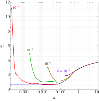
Figure 3: Position of the singularity $y_{I}$ as a function of the effective gravitational coupling $\kappa$.
Left: The position of the singularity at leading-order in RB, which converges to a value $y_{I}=0.602$ when $\kappa\ll 1$.
Right: The position of the singularity at leading-order in GRB, for large $f$ approaching $M_{P}$; the blue, red, green, brown, and purple correspond to log${}_{10}(\delta)=-6,-4,-3,-2,-1$ respectively. For sufficiently small $f$, $y_{I}$ converges to the value $y_{I}=0.602$ at small $\kappa$. The filled dots correspond to a cutoff of the solutions at the value $\Delta=1/\sqrt{2}$.

To determine the effect of gravity on the singularity, observe that under spherical symmetry, we can rewrite Eq. (4) as

$$b(x) =-\frac{1}{8\pi}\left[\int d^{3}x^{\prime}\frac{Y(x^{\prime})^{2}}{|\vec{x}-\vec{x}^{\prime}|}\right]$$

$$=-\frac{1}{8\pi}\int dx^{\prime}\,x^{\prime 2}\,Y(x^{\prime})^{2}\int dc_{\theta}d\phi\frac{1}{\sqrt{x^{2}+x^{\prime 2}-2\,x\,x^{\prime}\,c_{\theta}}}$$

$$=-\frac{1}{4}\left[\int_{0}^{x}dx^{\prime}\frac{x^{\prime 2}\,Y(x^{\prime})^{2}}{2\,x}+\int_{x}^{\infty}dx^{\prime}\,\frac{x^{\prime}\,Y(x^{\prime})^{2}}{2}\right].$$ (15)

Then substituting the ansatz of Eq. (14) for $Y(x)$ we can perform the integrals explicitly; we find

$$b_{s}(x) =-\frac{A^{2}}{16}\frac{\tan^{-1}\left(\frac{x}{y_{I}}\right)}{x\,y_{I}}.$$ (16)

Of course, the combination $Y_{s}$ and $b_{s}$ satisfies the Poisson equation Eby et al. (2018c)

$$\nabla_{x}^{2}\,b_{s}(x)=\frac{1}{2}Y_{s}(x)^{2}.$$ (17)

Thus we can see that the solution for $b(x)$ near the singularity at $x=i\,y_{I}$ is regular.

We now Taylor expand the wavefunction and gravitational potential around $x=0$, as

$$Y(x)=\sum_{n=0}^{\infty}\eta_{n}\,x^{2n},\qquad b(x)=\sum_{n=0}^{\infty}\beta_{n}\,x^{2n}.$$ (18)

Evaluating the equations of motion (3-4), we obtain recursion relations among the expansion parameters $\eta_{n}$ and $\beta_{n}$; for example, the coefficient multiplying $x^{2n}$ in Eq. (3) must evaluate to zero, which implies

$$(2n+2)(2n+1)\eta_{n+1} +4(n+1)\eta_{n+1}$$

$$+\frac{1}{8}\sum_{i,j\geq 0}\eta_{i}\eta_{j}\eta_{n-i-j}-\eta_{n}$$

$$-\kappa\sum_{i\geq 0}\beta_{i}\,\eta_{n-i}=0,$$ (19)

and similarly for $\beta_{n}$ and Eq. (4). We therefore leave $\eta_{0}$ and $\beta_{0}$ as free parameters and iteratively solve for $\eta_{n>0}$ and $\beta_{n>0}$ using these recursion relations, truncating at some large maximum integer in the expansion. The first-order terms in the expansions imply the coefficients

$$\eta_{1} =\frac{1}{6}\left[(1+\beta_{0}\,\kappa)\eta_{0}-\frac{\eta_{0}^{3}}{8}\right],$$

$$\beta_{1} =\frac{\eta_{0}^{2}}{12},$$

whereas the second order implies

$$\eta_{2} =\frac{1}{7680}\left[64\eta_{0}(1+\beta_{0}\,\kappa)^{2}-32\eta_{0}^{3}(1-\kappa+\beta_{0}\,\kappa)+3\eta_{0}^{5}\right],$$

$$\beta_{2} =\frac{1}{960}\left[8\eta_{0}^{2}(1+\beta_{0}\,\kappa)-\eta_{0}^{4}\right],$$

and so on.

We can then match Eq. (14) and Eq. (18) to obtain relations for $A$ and $y_{I}$ in terms of the parameters $\eta_{n}$; at $n$th order in the expansion, we obtain Eby et al. (2016b)

$$A =(-1)^{n}\,\eta_{n}\,y_{I}^{2n+2},$$ (20)

$$y_{I} =\sqrt{-\frac{\eta_{n-1}}{\eta_{n}}}.$$ (21)

Noting that using the recursion relations above, we have $\eta_{n}=\eta_{n}(\eta_{0},\beta_{0},\kappa)$, we can take a given solution and evaluate the position of the singularity $y_{I}(\eta_{0},\beta_{0},\kappa)$. In the limit $\kappa\to 0$ (gravitational decoupling), we recover the result of Eby et al. (2016b) that $A=8\,y_{I}$ and $y_{I}=0.602$. More generally at non-zero $\kappa$, we find $A=8\,y_{I}$ still holds, and illustrate the position of the singularity $y_{I}$ in the left panel of Figure 3.

A.2 Position of the Singularity in GRB

We turn now to the structure of the essential singularity including relativistic corrections, using the Generalized Ruffini-Bonazzola (GRB) formalism. The equation of motion for $Y(x)$ at next-to-leading order in the GRB formalism is Eq. (6). Using the recursion procedure above, we can determine the singularity structure of this equation as well. There are small modifications to the coefficient relations, e.g. $\eta_{1}$ in Eq. (A.1) is modified at ${\mathcal{O}}(\Delta^{2})$ as

$$\eta_{1}=\frac{1}{6}\left[(1+\beta_{0}\,\kappa)\eta_{0}-\frac{\eta_{0}^{3}}{8}+\frac{3}{512}\Delta^{2}\,\eta_{0}^{5}\right],$$ (22)

but the basic procedure is the same as above.

The GRB equation of motion depends on an additional parameter $\Delta$ in addition to $\kappa$, though at fixed $\Delta$ we trade the latter for $\delta=\Delta^{2}\,\kappa$. Therefore we characterize our solutions by the input parameters $\{\eta_{0},\beta_{0},\Delta,\delta\}$. We solved the GRB equation over a large range inside the bounds $10^{-4}\leq\Delta\leq 1/\sqrt{2}$ and $10^{-6}\leq\delta\leq 10^{-1}$ (this corresponds to $10^{-4}\lesssim\kappa\lesssim 10^{3}$); at the largest values of $\Delta$ we expect the higher-order contributions in GRB to be very relevant, and worse yet, such solutions are unphysical due to extremely high binding energies Eby et al. (2019). Still, we can analyze the structure of solutions as an academic exercise, and we will see that solutions with very large values of $\Delta$ are not phenomenologically relevant anyway due to fast decay rates.

In the right panel of Figure 3, we illustrate the shift in the singularity position for different choices of $\delta$, with the goal of approaching $f={\mathcal{O}}(M_{P})$. We see that, as expected, when $f$ is sufficiently small (given by the blue curve, or $f\lesssim 2.4\times 10^{15}$ GeV), the singularity is unaffected by the GRB correction over the full range of $\kappa$ we analyzed. As $f$ increases, the deviation in the singularity point appears at larger values of $\kappa$, though at the same time the cutoff at $\Delta=1/\sqrt{2}$ (given by the circles in the Figure) reduces the relevant physical range.

Figure 4: Comparison of different calculation methods for $I_{3}(\Delta)$: From residue theorem (blue); from numerical integration over $Y^{3}$ (red); from numerical integration over $J_{3}(\Delta\,Y)$ (green); and our final estimation (black) which interpolates between the blue curve at small $\Delta$ and the green curve at large $\Delta$. The choices of $\delta$ are $\delta=10^{-1}$ (top left), $\delta=10^{-2}$ (top right), $\delta=10^{-3}$ (bottom left), and $\delta=10^{-4}$ (bottom right).

We can now proceed to evaluate the lifetime of axion stars at large $f$ and moderate $\Delta$, at leading-order in GRB. With the position of the singularity $y_{I}$ in hand, we can use the residue theorem to compute $I_{3}$ in Eq. (13) and find

$$I_{3}(\Delta)\simeq i\,\frac{32\,\pi}{3}\frac{y_{I}}{\Delta}\exp\left(-\frac{k_{3}\,y_{I}}{\Delta}\right)\qquad{\rm(``Residue")},$$ (23)

which depends exponentially both on the inverse of the binding energy parameter $1/\Delta$ and the position of the singularity $y_{I}$.

However, note that at large $\Delta$ the result in Eq (23) will not be correct, as the application of the residue theorem assumed the validity of Eq. (13). When the product $\Delta\,Y(x)$ is large, we must not expand the Bessel function $J_{3}(\Delta\,Y(x))$ in Eq. (A.1); fortunately, it is in this range that the integrand does not oscillate fast and we can integrate $I_{3}$ directly. To briefly summarize:

• The analytic “Residue” result of Eq. (23) is applicable at low $\Delta\lesssim 0.1$;

• The numerical result “Bessel” from integrating $J_{3}$ in Eq. (A.1) is applicable at the largest $\Delta\sim\Delta_{\rm max}=1/\sqrt{2}$;

• Both should roughly agree, with each other and with Eq. (13) (“$Y^{3}$”), in an intermediate range $0.1\lesssim\Delta\lesssim\Delta_{\rm max}$.

We illustrate the results of these estimations (blue for residues, green for Bessel, red for $Y^{3}$) in Figure 4. The black line, which we use to calculate the decay rate in the next section, interpolates between Eq. (23) at low $\Delta$ and Eq. (A.1) at high $\Delta$; when in doubt we used the smaller estimation of $|I_{3}|$ to make a conservative estimation of the decay rate.

Figure 5: The single-annihilation decay rate $\Gamma_{3}$ for $\delta=10^{-4},10^{-3},10^{-2},10^{-1}$ (respectively the red, green, brown, and purple curves). In the left panel, the particle mass is fixed to $10^{-5}$ eV, whereas in the right panel $m$ is varied on each order of magnitude between $10^{-20}-1$ eV (lines from top to bottom of each band).

A.3 Decay Rate and Lifetime

The decay rate for a single annihilation process is given by Eby et al. (2016b, 2018a)

$$\Gamma_{3}(\Delta)=\frac{f^{2}}{2\pi k_{3}\,m}|I_{3}(\Delta)|^{2}.$$ (24)

We show the resulting rate of annihilations/sec in Fig. 5 for different choices of $\delta=10^{-4},10^{-3},10^{-2},10^{-1}$ (the red, green, brown, and purple curves, respectively). In the left panel we have fixed the axion mass $m=10^{-5}$ eV, whereas we vary $m$ in the right panel between $m=1$ eV (bottom of each band) and $m=10^{-20}$ eV (top). We observe a very rapid increase of the decay rate, from extremely small values $\ll 1$ annihilation/sec to greater than $10^{40}$ annihilations/sec around (for example) $\Delta\simeq 0.03$ for $\delta=10^{-4}$. This increase occurs at slightly higher values of $\Delta$ for larger $m$ or for larger $f$ (i.e. larger $\delta$).

The lifetime is proportional to $|I_{3}|^{-2}\propto\exp(y_{I}/\Delta)$, implying that dilute axion stars (corresponding to the smallest allowed $\Delta$) may be stable and survive longer than the age of the universe. However, this has only been explicitly investigated at small values of $f$, and we have seen that naive extrapolation of such results to large $f$ may not be appropriate. Indeed, we find that contrary to conventional wisdom about axion stars, the lifetime for $f\gtrsim 10^{17}$ GeV is shorter than the age of the universe even on the dilute branch, as explained below.

We estimate the lifetime numerically as follows. In a region of parameter space where the decay rate is large, we may approximate it as constant, as the axion star explodes in a rapid Bosenova of relativistic particles; we call this the instantaneous approximation. In that case (assuming a constant decay rate), the timescale for the evaporation of the star would be

$$\tau_{0}=\frac{N}{3}\,\frac{1}{\Gamma_{3}}\simeq\frac{2\pi\,k_{3}}{3\,f^{2}}\frac{M(\Delta)}{|I_{3}(\Delta)|^{2}},$$ (25)

where the prefactor $N/3$ is the number of annihilations necessary to completely deplete the star (for each annihilation, $3$ bound axions are lost). Then, because $M$ has a one-to-one relationship with $\Delta$, we can compute the decay timescale uniquely as a function of $\Delta$. In practice we use the full solution for $M(\Delta)$ in the numerical results, which is illustrated in Fig. 6. Note that the lifetime in Eq. (25) is identical to the one used in Eby et al. (2016b, 2018a), but here it is evaluated in the instantaneous limit; we clarify the difference at the end of this section.

Using fits on each branch of axion stars, we obtain an analytic form for the lifetime which may help guide the reader’s intuition. Firstly, in Eby et al. (2016b, 2018a), we noted that (at small $f\simeq 10^{12}$ GeV) the decay rate was exponentially small on the dilute branch and that the lifetime only became short on the transition branch; in that case, the relationship between $M$ and $\Delta$ is given by

$$M(\Delta)=\frac{y_{t}}{\Delta}\frac{f^{2}}{m}\qquad\qquad{\rm(Transition\,\,branch)},$$ (26)

with $y_{t}\simeq 75.4$ is determined by fitting the mass function shown in Fig. 6 Eby et al. (2018a). Then the timescale for instantaneous decay is

$$\tau_{0}\simeq\frac{2\pi\,k_{3}\,y_{t}}{3\,m\,\Delta}\frac{1}{|I_{3}(\Delta)|^{2}} \approx\frac{447}{m\,\Delta}\frac{1}{|I_{3}(\Delta)|^{2}}$$

$${\rm(Transition\,\,branch)}.$$ (27)

Figure 6: Mass of axion stars as a function of $\Delta$, for different choices of $\delta$ (colors match those of Figure 5). The filled circles represent the endpoint of our set of solutions, at $\Delta=1/\sqrt{2}$.

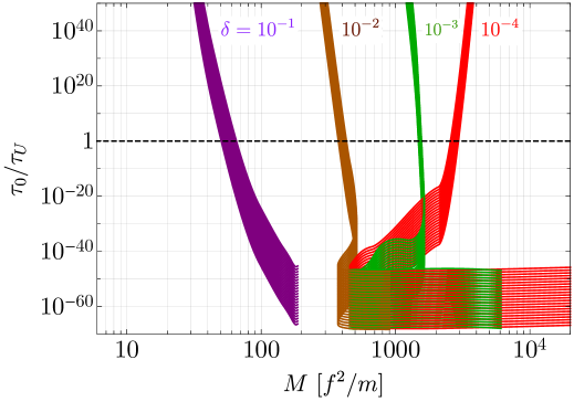
Figure 7: Lifetime of axion stars (in the instantaneous approximation), normalized to the universe lifetime $\tau_{U}$, as a function of total mass $M$, for different choices of $\delta$ (colors match those of Figure 5). The width of the curves represents choices of $m$ varied on each order of magnitude in the range $10^{-20}-1$ eV (lines from bottom to top of each band).

For large $f$, we find in this work that the decay timescale can, on the dilute branch, already be lower than the age of the universe, as $\Delta$ becomes large before the crossover point. In that case the mass function is

$$M(\Delta)=y_{d}\,\Delta\,\frac{f^{2}}{m}\qquad\qquad{\rm(Dilute\,\,branch)}$$ (28)

with $y_{d}=1.75\times 8\pi/\delta$ (found by fitting the curves in Fig. 6), and the lifetime takes the form

$$\tau_{0}\simeq\frac{2\pi\,k_{3}\,y_{d}\,\Delta}{3\,m}\frac{1}{|I_{3}(\Delta)|^{2}}\approx\frac{261\,\Delta}{m\,\delta}\frac{1}{|I_{3}(\Delta)|^{2}}$$

$$\qquad\qquad{\rm(Dilute\,\,branch)}.$$ (29)

Due to the rapid turn-on of the decay rate, aside from a very narrow region near $\tau_{0}\simeq\tau_{U}$, the lifetime of axion stars is either (i) so long that the star can be treated as stable with a conserved particle number $N$, or (ii) so short that the star decays almost instantly. In the latter case, the instantaneous approximation above seems very well-justified, as the relaxation time for the axion star to remain in its equilibrium configuration at each instant as it evolves will likely be much longer than the decay timescale $\tau_{0}$. Therefore, we use the instantaneous case to define the crossover from stability to instability under decay which we describe in the Main Text. The result for the instantaneous lifetime as a function of $M$ and $\delta$ is given in Fig. 7

Appendix B Comparison to Previous Work

Below, we review previous work on the decay of axion stars, as well as their possible collapse to black holes, and compare these results with our own.

Decay Rate: In this work we computed the lifetime of axion stars using an instantaneous approximation. Although we feel this approximation is justified, the arguments above fall short of a proof, as the relaxation timescale has not been worked out in detail. In a situation in which the axion star tracks its equilibrium configuration as it decays, one should integrate the decay rate as a function of $M$ from an initial $M_{0}$ to some smaller final value $M_{f}$, i.e.

$$\tau=\frac{1}{3}\int\frac{dN}{\Gamma_{3}}\simeq\frac{2\pi\,k_{3}}{3\,f^{2}}\int_{M_{0}}^{M_{f}}\frac{dM}{|I_{3}(\Delta)|^{2}}.$$ (30)

This formulation was used by us in previous work to determine the lifetime of axion stars on the transition branch Eby et al. (2016b, 2018a). We found that on the transition branch, $M\propto 1/\Delta$ but $I_{3}(\Delta)\propto\exp\left(-1/\Delta\right)$, and so $dM/|I_{3}(\Delta)|^{2}\ggg 1$ when $\Delta\ll 1$. In that case, the lifetime integral is dominated by the smallest $M$ in the integration range (that is, $M_{f}$), and the result was given by Eq. (11) with $M=M_{f}$.

An important difference between the adiabatic and instantaneous approximations is the scaling of the lifetime with the parameter $\Delta$. For example, on the transition branch (where gravity decouples) at small $\Delta$ (where Eq. (23) is appropriate), the adiabatic case in Eq. (30) gives $\tau\sim a_{A}\,(\Delta^{2}/m)\,\exp(c/\Delta)$, where $a_{A}$ and $c$ are constants, as found in Eby et al. (2016b, 2018a) (see Eq. (11)). On the other hand, the instantaneous case of Eq. (A.3) gives $\tau\sim a_{I}\,(\Delta/m)\,\exp(c/\Delta)$, where $a_{I}$ is another constant. The latter is precisely the scaling found in previous investigations using classical field theory; see e.g. Eq. (24) of Hertzberg (2010) or Eq. (50) of Grandclement et al. (2011). In all cases, the prefactor retains no explicit dependence on $f$.

ULDM Simulations: In these simulations Schive et al. (2014b, a); Mocz et al. (2017); Veltmaat et al. (2020); Nori and Baldi (2020), axion stars form with very large masses $M$ due to the smallness of the particle mass $m\simeq 10^{-22}$ eV; in large halos of total mass $M_{h}\gtrsim 10^{9}M_{\odot}$, the axion star mass appears to follow a now well-known relation Schive et al. (2014b); Bar et al. (2018)

$$M=1.4\times 10^{9}M_{\odot}\left(\frac{10^{-22}\,{\rm eV}}{m}\right)\left(\frac{M_{h}}{10^{12}M_{\odot}}\right)^{1/3}.$$ (31)

Comparing to the maximum gravitationally-stable mass $M_{\rm max}=10.2\,M_{P}\,f/m$, we see that

$$\frac{M}{M_{\rm max}}\simeq 0.013\left(\frac{10^{17}\,{\rm GeV}}{f}\right)\left(\frac{M_{h}}{10^{12}M_{\odot}}\right)^{1/3},$$ (32)

so in the largest halos simulated, where $M_{h}\simeq 10^{12}M_{\odot}$, a typical ULDM candidate with $f=10^{17}$ GeV will form an axion star core with mass $\sim 80$ times below its maximum mass. If axion stars can accrete enough mass after formation to cover this gap, they run the risk of not only collapsing but also decaying, because as illustrated in Fig. 1 the decay instability sets in also in the same parameter range.

Collapse Simulations: Other simulations have probed the fate of axion stars at large $f={\mathcal{O}}(M_{P})$ by evolving the classical equations of motion Helfer et al. (2017); Widdicombe et al. (2018). One of the purposes of these simulations was to determine under which conditions an axion star might collapse directly to a black hole; their analysis suggests a triple point in the axion star phase diagram at $f_{TP}\simeq 0.3\tilde{M}_{P}$ and $M_{TP}\simeq 2.4\tilde{M}_{P}^{2}/m$, which is $\delta_{TP}=0.09$ and $M_{TP}=(2.4/\delta)(f^{2}/m)=26.6\,f^{2}/m$ in the notation of this paper. We confirm some of these results but not all, as explained below.

The “dispersal region” in the phase diagram of Helfer et al. (2017), which we understand to be the transition branch of solutions in the equations of motion, disappears above the triple point at $f\gtrsim 0.3\tilde{M}_{p}$. We observe this as the disappearance of the transition branch, which occurs for $\delta\gtrsim 10^{-1}$ (the purple curve in Fig. 1), roughly confirming their result for $f_{TP}$; we do not, however, confirm the mass at the triple point, which is a factor of few larger in their result compared to ours. It is possible this difference originates in the use of the “classical” equations of motion in Helfer et al. (2017) (i.e. a cosine rather than a Bessel function in the self-interaction potential); we have pointed out previous that this change, when evaluated on the transition branch of axion stars, leads to differences compared to the semi-classical analysis we have used here Eby et al. (2019).

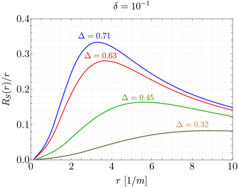
Figure 8: The ratio of the Schwarzschild radius $R_{S}(r)$ to the radius in the axion star $r$, for radii less than or equal to the total radius $R_{99}$, at $\delta=10^{-1}$ and at different (labeled) values of $\Delta$. When the ratio is $\ll 1$, the star is far from the General Relativistic limit.

Secondly, in spite of analyzing states at large binding energy, we find General Relativistic effects to be negligible everywhere, and therefore do not confirm the formation of black holes observed in Helfer et al. (2017); Widdicombe et al. (2018). For each solution at large $\delta$, we confirm first that the Schwarzschild radius $R_{S}=2\,G\,M$ is always much smaller than the radius of the star $R_{99}$. We further checked that the condition $R_{S}(r)=2\,G\,{\mathcal{M}}(r)<r$ is satisfied inside the star at every $r<R_{99}$, as most of the density is in the inner region. For $\delta=0.1$ (near the triple point of Helfer et al. (2017)), we see in Fig. 8 that the ratio $R_{S}(r)/r\ll 1$ for all points in our solution space, and therefore these states are not black holes. Note however, that the analyses of Helfer et al. (2017); Widdicombe et al. (2018) were dynamical, focusing on the collapse of axionic objects, whereas ours is static by construction; the results of this work apply to structurally stable (or metastable) configurations only. In those works the initial profiles were also far from the physical axion star profiles we analyze here. These factors may account for any discrepancy between the two results, though a more thorough investigation may be warranted.

References

- Peccei and Quinn (1977a) R.D. Peccei and Helen R. Quinn. CP Conservation in the Presence of Instantons. Phys. Rev. Lett., 38:1440–1443, 1977a. doi: 10.1103/PhysRevLett.38.1440.
- Peccei and Quinn (1977b) R.D. Peccei and Helen R. Quinn. Constraints Imposed by CP Conservation in the Presence of Instantons. Phys. Rev. D, 16:1791–1797, 1977b. doi: 10.1103/PhysRevD.16.1791.
- Weinberg (1978) Steven Weinberg. A New Light Boson? Phys. Rev. Lett., 40:223–226, 1978. doi: 10.1103/PhysRevLett.40.223.
- Wilczek (1978) Frank Wilczek. Problem of Strong and Invariance in the Presence of Instantons. Phys. Rev. Lett., 40:279–282, 1978. doi: 10.1103/PhysRevLett.40.279.
- Dine et al. (1981) Michael Dine, Willy Fischler, and Mark Srednicki. A Simple Solution to the Strong CP Problem with a Harmless Axion. Phys. Lett. B, 104:199–202, 1981. doi: 10.1016/0370-2693(81)90590-6.
- Zhitnitsky (1980) A.R. Zhitnitsky. On Possible Suppression of the Axion Hadron Interactions. (In Russian). Sov. J. Nucl. Phys., 31:260, 1980.
- Kim (1979) Jihn E. Kim. Weak Interaction Singlet and Strong CP Invariance. Phys. Rev. Lett., 43:103, 1979. doi: 10.1103/PhysRevLett.43.103.
- Shifman et al. (1980) Mikhail A. Shifman, A.I. Vainshtein, and Valentin I. Zakharov. Can Confinement Ensure Natural CP Invariance of Strong Interactions? Nucl. Phys. B, 166:493–506, 1980. doi: 10.1016/0550-3213(80)90209-6.
- Turner (1983) Michael S. Turner. Coherent Scalar Field Oscillations in an Expanding Universe. Phys. Rev. D, 28:1243, 1983. doi: 10.1103/PhysRevD.28.1243.
- Press et al. (1990) William H. Press, Barbara S. Ryden, and David N. Spergel. Single Mechanism for Generating Large Scale Structure and Providing Dark Missing Matter. Phys. Rev. Lett., 64:1084, 1990. doi: 10.1103/PhysRevLett.64.1084.
- Sin (1994) Sang-Jin Sin. Late time cosmological phase transition and galactic halo as Bose liquid. Phys. Rev. D, 50:3650–3654, 1994. doi: 10.1103/PhysRevD.50.3650.
- Hu et al. (2000) Wayne Hu, Rennan Barkana, and Andrei Gruzinov. Cold and fuzzy dark matter. Phys. Rev. Lett., 85:1158–1161, 2000. doi: 10.1103/PhysRevLett.85.1158.
- Goodman (2000) Jeremy Goodman. Repulsive dark matter. New Astron., 5:103, 2000. doi: 10.1016/S1384-1076(00)00015-4.
- Peebles (2000) P.J.E. Peebles. Fluid dark matter. Astrophys. J., 534:L127, 2000. doi: 10.1086/312677.
- Amendola and Barbieri (2006) Luca Amendola and Riccardo Barbieri. Dark matter from an ultra-light pseudo-Goldsone-boson. Phys. Lett. B, 642:192–196, 2006. doi: 10.1016/j.physletb.2006.08.069.
- Li et al. (2014) Bohua Li, Tanja Rindler-Daller, and Paul R. Shapiro. Cosmological Constraints on Bose-Einstein-Condensed Scalar Field Dark Matter. Phys. Rev. D, 89(8):083536, 2014. doi: 10.1103/PhysRevD.89.083536.
- Marsh (2016) David J. E. Marsh. Axion Cosmology. Phys. Rept., 643:1–79, 2016. doi: 10.1016/j.physrep.2016.06.005.
- Hui et al. (2017) Lam Hui, Jeremiah P. Ostriker, Scott Tremaine, and Edward Witten. Ultralight scalars as cosmological dark matter. Phys. Rev. D, 95(4):043541, 2017. doi: 10.1103/PhysRevD.95.043541.
- Lee (2018) Jae-Weon Lee. Brief History of Ultra-light Scalar Dark Matter Models. EPJ Web Conf., 168:06005, 2018. doi: 10.1051/epjconf/201816806005.
- Eby et al. (2016a) Joshua Eby, Madelyn Leembruggen, Peter Suranyi, and L.C.R. Wijewardhana. Collapse of Axion Stars. JHEP, 12:066, 2016a. doi: 10.1007/JHEP12(2016)066.
- Visinelli et al. (2018) Luca Visinelli, Sebastian Baum, Javier Redondo, Katherine Freese, and Frank Wilczek. Dilute and dense axion stars. Phys. Lett. B, 777:64–72, 2018. doi: 10.1016/j.physletb.2017.12.010.
- Grin et al. (2019) Daniel Grin, Mustafa A. Amin, Vera Gluscevic, Renée Hlǒzek, David J.E. Marsh, Vivian Poulin, Chanda Prescod-Weinstein, and Tristan L. Smith. Gravitational probes of ultra-light axions. arXiv: 1904.09003, 4 2019.
- Preskill et al. (1983) John Preskill, Mark B. Wise, and Frank Wilczek. Cosmology of the Invisible Axion. Phys. Lett. B, 120:127–132, 1983. doi: 10.1016/0370-2693(83)90637-8.
- Abbott and Sikivie (1983) L.F. Abbott and P. Sikivie. A Cosmological Bound on the Invisible Axion. Phys. Lett. B, 120:133–136, 1983. doi: 10.1016/0370-2693(83)90638-X.
- Dine and Fischler (1983) Michael Dine and Willy Fischler. The Not So Harmless Axion. Phys. Lett. B, 120:137–141, 1983. doi: 10.1016/0370-2693(83)90639-1.
- Kaup (1968) David J. Kaup. Klein-Gordon Geon. Phys. Rev., 172:1331–1342, 1968. doi: 10.1103/PhysRev.172.1331.
- Ruffini and Bonazzola (1969) Remo Ruffini and Silvano Bonazzola. Systems of selfgravitating particles in general relativity and the concept of an equation of state. Phys. Rev., 187:1767–1783, 1969. doi: 10.1103/PhysRev.187.1767.
- Breit et al. (1984) J.D. Breit, S. Gupta, and A. Zaks. Cold bose stars. Physics Letters B, 140(5):329 – 332, 1984. ISSN 0370-2693. doi: https://doi.org/10.1016/0370-2693(84)90764-0. URL http://www.sciencedirect.com/science/article/pii/0370269384907640.
- Colpi et al. (1986) M. Colpi, S.L. Shapiro, and I. Wasserman. Boson Stars: Gravitational Equilibria of Selfinteracting Scalar Fields. Phys. Rev. Lett., 57:2485–2488, 1986. doi: 10.1103/PhysRevLett.57.2485.
- Seidel and Suen (1990) Edward Seidel and Wai-Mo Suen. Dynamical Evolution of Boson Stars. 1. Perturbing the Ground State. Phys. Rev. D, 42:384–403, 1990. doi: 10.1103/PhysRevD.42.384.
- Friedberg et al. (1987) R. Friedberg, T.D. Lee, and Y. Pang. Scalar Soliton Stars and Black Holes. Phys. Rev. D, 35:3658, 1987. doi: 10.1103/PhysRevD.35.3658.
- Seidel and Suen (1991) E. Seidel and W.M. Suen. Oscillating soliton stars. Phys. Rev. Lett., 66:1659–1662, 1991. doi: 10.1103/PhysRevLett.66.1659.
- Liddle and Madsen (1992) Andrew R. Liddle and Mark S. Madsen. The Structure and formation of boson stars. Int. J. Mod. Phys. D, 1:101–144, 1992. doi: 10.1142/S0218271892000057.
- Lee and Pang (1992) T.D. Lee and Y. Pang. Nontopological solitons. Phys. Rept., 221:251–350, 1992. doi: 10.1016/0370-1573(92)90064-7.
- Chavanis (2011) Pierre-Henri Chavanis. Mass-radius relation of Newtonian self-gravitating Bose-Einstein condensates with short-range interactions: I. Analytical results. Phys. Rev. D, 84:043531, 2011. doi: 10.1103/PhysRevD.84.043531.
- Chavanis and Delfini (2011) P.H. Chavanis and L. Delfini. Mass-radius relation of Newtonian self-gravitating Bose-Einstein condensates with short-range interactions: II. Numerical results. Phys. Rev. D, 84:043532, 2011. doi: 10.1103/PhysRevD.84.043532.
- Braaten and Zhang (2019) Eric Braaten and Hong Zhang. Colloquium : The physics of axion stars. Rev. Mod. Phys., 91(4):041002, 2019. doi: 10.1103/RevModPhys.91.041002.
- Zhang (2019) Hong Zhang. Axion Stars. Symmetry, 12(1):25, 2019. doi: 10.3390/sym12010025.
- Eby et al. (2019) Joshua Eby, Madelyn Leembruggen, Lauren Street, Peter Suranyi, and L.C. R. Wijewardhana. Global view of QCD axion stars. Phys. Rev. D, 100(6):063002, 2019. doi: 10.1103/PhysRevD.100.063002.
- Eby et al. (2016b) Joshua Eby, Peter Suranyi, and L.C.R. Wijewardhana. The Lifetime of Axion Stars. Mod. Phys. Lett. A, 31(15):1650090, 2016b. doi: 10.1142/S0217732316500905.
- Eby et al. (2018a) Joshua Eby, Michael Ma, Peter Suranyi, and L.C.R. Wijewardhana. Decay of Ultralight Axion Condensates. JHEP, 01:066, 2018a. doi: 10.1007/JHEP01(2018)066.
- Schive et al. (2014a) Hsi-Yu Schive, Ming-Hsuan Liao, Tak-Pong Woo, Shing-Kwong Wong, Tzihong Chiueh, Tom Broadhurst, and W.-Y. Pauchy Hwang. Understanding the Core-Halo Relation of Quantum Wave Dark Matter from 3D Simulations. Phys. Rev. Lett., 113(26):261302, 2014a. doi: 10.1103/PhysRevLett.113.261302.
- Levkov et al. (2018) D.G. Levkov, A.G. Panin, and I.I. Tkachev. Gravitational Bose-Einstein condensation in the kinetic regime. Phys. Rev. Lett., 121(15):151301, 2018. doi: 10.1103/PhysRevLett.121.151301.
- Eggemeier and Niemeyer (2019) Benedikt Eggemeier and Jens C. Niemeyer. Formation and mass growth of axion stars in axion miniclusters. Phys. Rev. D, 100(6):063528, 2019. doi: 10.1103/PhysRevD.100.063528.
- Kirkpatrick et al. (2020) Kay Kirkpatrick, Anthony E. Mirasola, and Chanda Prescod-Weinstein. Relaxation times for Bose-Einstein condensation in axion miniclusters. arXiv: 2007.07438, 7 2020.
- Hertzberg and Schiappacasse (2018) Mark P. Hertzberg and Enrico D. Schiappacasse. Dark Matter Axion Clump Resonance of Photons. JCAP, 11:004, 2018. doi: 10.1088/1475-7516/2018/11/004.
- Hertzberg et al. (2020a) Mark P. Hertzberg, Yao Li, and Enrico D. Schiappacasse. Merger of Dark Matter Axion Clumps and Resonant Photon Emission. arXiv: 2005.02405, 5 2020a.
- Levkov et al. (2020) D.G. Levkov, A.G. Panin, and I.I. Tkachev. Radio-emission of axion stars. Phys. Rev. D, 102(2):023501, 2020. doi: 10.1103/PhysRevD.102.023501.
- Amin and Mou (2020) Mustafa A. Amin and Zong-Gang Mou. Electromagnetic Bursts from Mergers of Oscillons in Axion-like Fields. arXiv: 2009.11337, 9 2020.
- Croon et al. (2020a) Djuna Croon, David McKeen, and Nirmal Raj. Gravitational microlensing by dark matter in extended structures. Phys. Rev. D, 101(8):083013, 2020a. doi: 10.1103/PhysRevD.101.083013.
- Prabhu (2020) Anirudh Prabhu. Optical Lensing by Axion Stars: Observational Prospects with Radio Astrometry. arXiv: 2006.10231, 6 2020.
- Croon et al. (2020b) Djuna Croon, David McKeen, Nirmal Raj, and Zihui Wang. Subaru through a different lens: microlensing by extended dark matter structures. arXiv: 2007.12697, 7 2020b.
- Eby et al. (2015) Joshua Eby, Peter Suranyi, Cenalo Vaz, and L.C.R. Wijewardhana. Axion Stars in the Infrared Limit. JHEP, 03:080, 2015. doi: 10.1007/JHEP11(2016)134. [Erratum: JHEP 11, 134 (2016)].
- Schiappacasse and Hertzberg (2018) Enrico D. Schiappacasse and Mark P. Hertzberg. Analysis of Dark Matter Axion Clumps with Spherical Symmetry. JCAP, 01:037, 2018. doi: 10.1088/1475-7516/2018/01/037. [Erratum: JCAP 03, E01 (2018)].
- Braaten et al. (2016a) Eric Braaten, Abhishek Mohapatra, and Hong Zhang. Dense Axion Stars. Phys. Rev. Lett., 117(12):121801, 2016a. doi: 10.1103/PhysRevLett.117.121801.
- Kolb and Tkachev (1994) Edward W. Kolb and Igor I. Tkachev. Nonlinear axion dynamics and formation of cosmological pseudosolitons. Phys. Rev. D, 49:5040–5051, 1994. doi: 10.1103/PhysRevD.49.5040.
- Di Vecchia and Veneziano (1980) P. Di Vecchia and G. Veneziano. Chiral Dynamics in the Large n Limit. Nucl. Phys. B, 171:253–272, 1980. doi: 10.1016/0550-3213(80)90370-3.
- Grilli di Cortona et al. (2016) Giovanni Grilli di Cortona, Edward Hardy, Javier Pardo Vega, and Giovanni Villadoro. The QCD axion, precisely. JHEP, 01:034, 2016. doi: 10.1007/JHEP01(2016)034.
- Gorghetto et al. (2020) Marco Gorghetto, Edward Hardy, and Giovanni Villadoro. More Axions from Strings. arXiv: 2007.04990, 7 2020.
- Bonnefoy et al. (2019) Quentin Bonnefoy, Emilian Dudas, and Stefan Pokorski. Axions in a highly protected gauge symmetry model. Eur. Phys. J. C, 79(1):31, 2019. doi: 10.1140/epjc/s10052-018-6528-z.
- Arvanitaki et al. (2020) Asimina Arvanitaki, Savas Dimopoulos, Marios Galanis, Luis Lehner, Jedidiah O. Thompson, and Ken Van Tilburg. Large-misalignment mechanism for the formation of compact axion structures: Signatures from the QCD axion to fuzzy dark matter. Phys. Rev. D, 101(8):083014, 2020. doi: 10.1103/PhysRevD.101.083014.
- Svrcek and Witten (2006) Peter Svrcek and Edward Witten. Axions In String Theory. JHEP, 06:051, 2006. doi: 10.1088/1126-6708/2006/06/051.
- Cicoli et al. (2012) Michele Cicoli, Mark Goodsell, and Andreas Ringwald. The type IIB string axiverse and its low-energy phenomenology. JHEP, 10:146, 2012. doi: 10.1007/JHEP10(2012)146.
- Arvanitaki et al. (2010) Asimina Arvanitaki, Savas Dimopoulos, Sergei Dubovsky, Nemanja Kaloper, and John March-Russell. String Axiverse. Phys. Rev. D, 81:123530, 2010. doi: 10.1103/PhysRevD.81.123530.
- Schive et al. (2014b) Hsi-Yu Schive, Tzihong Chiueh, and Tom Broadhurst. Cosmic Structure as the Quantum Interference of a Coherent Dark Wave. Nature Phys., 10:496–499, 2014b. doi: 10.1038/nphys2996.
- Mocz et al. (2017) Philip Mocz, Mark Vogelsberger, Victor H. Robles, Jesús Zavala, Michael Boylan-Kolchin, Anastasia Fialkov, and Lars Hernquist. Galaxy formation with BECDM – I. Turbulence and relaxation of idealized haloes. Mon. Not. Roy. Astron. Soc., 471(4):4559–4570, 2017. doi: 10.1093/mnras/stx1887.
- Veltmaat et al. (2020) Jan Veltmaat, Bodo Schwabe, and Jens C. Niemeyer. Baryon-driven growth of solitonic cores in fuzzy dark matter halos. Phys. Rev. D, 101(8):083518, 2020. doi: 10.1103/PhysRevD.101.083518.
- Nori and Baldi (2020) Matteo Nori and Marco Baldi. Scaling relations of Fuzzy Dark Matter haloes I: individual systems in their cosmological environment. arXiv: 2007.01316, 7 2020.
- Banerjee et al. (2019) Abhishek Banerjee, Hyungjin Kim, and Gilad Perez. Coherent relaxion dark matter. Phys. Rev. D, 100(11):115026, 2019. doi: 10.1103/PhysRevD.100.115026.
- Clough et al. (2018) Katy Clough, Tim Dietrich, and Jens C. Niemeyer. Axion star collisions with black holes and neutron stars in full 3D numerical relativity. Phys. Rev. D, 98(8):083020, 2018. doi: 10.1103/PhysRevD.98.083020.
- Dietrich et al. (2019) Tim Dietrich, Francesca Day, Katy Clough, Michael Coughlin, and Jens Niemeyer. Neutron star–axion star collisions in the light of multimessenger astronomy. Mon. Not. Roy. Astron. Soc., 483(1):908–914, 2019. doi: 10.1093/mnras/sty3158.
- Eby et al. (2017) Joshua Eby, Madelyn Leembruggen, Peter Suranyi, and L.C.R. Wijewardhana. QCD Axion Star Collapse with the Chiral Potential. JHEP, 06:014, 2017. doi: 10.1007/JHEP06(2017)014.
- Levkov et al. (2017) D.G. Levkov, A.G. Panin, and I.I. Tkachev. Relativistic axions from collapsing Bose stars. Phys. Rev. Lett., 118(1):011301, 2017. doi: 10.1103/PhysRevLett.118.011301.
- Helfer et al. (2017) Thomas Helfer, David J. E. Marsh, Katy Clough, Malcolm Fairbairn, Eugene A. Lim, and Ricardo Becerril. Black hole formation from axion stars. JCAP, 03:055, 2017. doi: 10.1088/1475-7516/2017/03/055.
- Chavanis (2018) Pierre-Henri Chavanis. Phase transitions between dilute and dense axion stars. Phys. Rev. D, 98(2):023009, 2018. doi: 10.1103/PhysRevD.98.023009.
- Michel and Moss (2018) Florent Michel and Ian G. Moss. Relativistic collapse of axion stars. Phys. Lett. B, 785:9–13, 2018. doi: 10.1016/j.physletb.2018.07.063.
- Widdicombe et al. (2018) James Y. Widdicombe, Thomas Helfer, David J.E. Marsh, and Eugene A. Lim. Formation of Relativistic Axion Stars. JCAP, 10:005, 2018. doi: 10.1088/1475-7516/2018/10/005.
- Abbott et al. (2020) R. Abbott et al. GW190814: Gravitational Waves from the Coalescence of a 23 Solar Mass Black Hole with a 2.6 Solar Mass Compact Object. Astrophys. J., 896(2):L44, 2020. doi: 10.3847/2041-8213/ab960f.
- Barranco and Bernal (2011) J. Barranco and A. Bernal. Self-gravitating system made of axions. Phys. Rev. D, 83:043525, 2011. doi: 10.1103/PhysRevD.83.043525.
- Eby et al. (2018b) Joshua Eby, Peter Suranyi, and L.C.R. Wijewardhana. Expansion in Higher Harmonics of Boson Stars using a Generalized Ruffini-Bonazzola Approach, Part 1: Bound States. JCAP, 04:038, 2018b. doi: 10.1088/1475-7516/2018/04/038.
- Eby et al. (2018c) Joshua Eby, Madelyn Leembruggen, Lauren Street, Peter Suranyi, and L.C.R. Wijewardhana. Approximation methods in the study of boson stars. Phys. Rev. D, 98(12):123013, 2018c. doi: 10.1103/PhysRevD.98.123013.
- Mukaida et al. (2017) Kyohei Mukaida, Masahiro Takimoto, and Masaki Yamada. On Longevity of I-ball/Oscillon. JHEP, 03:122, 2017. doi: 10.1007/JHEP03(2017)122.
- Braaten et al. (2016b) Eric Braaten, Abhishek Mohapatra, and Hong Zhang. Nonrelativistic Effective Field Theory for Axions. Phys. Rev. D, 94(7):076004, 2016b. doi: 10.1103/PhysRevD.94.076004.
- Namjoo et al. (2018) Mohammad Hossein Namjoo, Alan H. Guth, and David I. Kaiser. Relativistic Corrections to Nonrelativistic Effective Field Theories. Phys. Rev. D, 98(1):016011, 2018. doi: 10.1103/PhysRevD.98.016011.
- Braaten et al. (2018) Eric Braaten, Abhishek Mohapatra, and Hong Zhang. Classical Nonrelativistic Effective Field Theories for a Real Scalar Field. Phys. Rev. D, 98(9):096012, 2018. doi: 10.1103/PhysRevD.98.096012.
- Croon et al. (2019) Djuna Croon, Jiji Fan, and Chen Sun. Boson Star from Repulsive Light Scalars and Gravitational Waves. JCAP, 04:008, 2019. doi: 10.1088/1475-7516/2019/04/008.
- Eby (2017) Joshua Armstrong Eby. Phenomenology and Astrophysics of Gravitationally-Bound Condensates of Axion-Like Particles. PhD thesis, Cincinnati U., 2017.
- Braaten et al. (2017) Eric Braaten, Abhishek Mohapatra, and Hong Zhang. Emission of Photons and Relativistic Axions from Axion Stars. Phys. Rev. D, 96(3):031901, 2017. doi: 10.1103/PhysRevD.96.031901.
- Hertzberg (2010) Mark P. Hertzberg. Quantum Radiation of Oscillons. Phys. Rev. D, 82:045022, 2010. doi: 10.1103/PhysRevD.82.045022.
- Grandclement et al. (2011) Philippe Grandclement, Gyula Fodor, and Peter Forgacs. Numerical simulation of oscillatons: extracting the radiating tail. Phys. Rev. D, 84:065037, 2011. doi: 10.1103/PhysRevD.84.065037.
- Hertzberg et al. (2020b) Mark P. Hertzberg, Fabrizio Rompineve, and Jessie Yang. Decay of Boson Stars with Application to Glueballs and Other Real Scalars. arXiv: 2010.07927, 10 2020b.
- Eby et al. (2018d) Joshua Eby, Madelyn Leembruggen, Peter Suranyi, and L.C.R. Wijewardhana. Stability of Condensed Fuzzy Dark Matter Halos. JCAP, 10:058, 2018d. doi: 10.1088/1475-7516/2018/10/058.
- Montero et al. (2015) Miguel Montero, Angel M. Uranga, and Irene Valenzuela. Transplanckian axions!? JHEP, 08:032, 2015. doi: 10.1007/JHEP08(2015)032.
- Kaplan and Rattazzi (2016) David E. Kaplan and Riccardo Rattazzi. Large field excursions and approximate discrete symmetries from a clockwork axion. Phys. Rev. D, 93(8):085007, 2016. doi: 10.1103/PhysRevD.93.085007.
- Fonseca et al. (2019) Nayara Fonseca, Benedict von Harling, Leonardo de Lima, and Camila S. Machado. Super-Planckian axions from near-conformality. Phys. Rev. D, 100(10):105019, 2019. doi: 10.1103/PhysRevD.100.105019.
- Zhang et al. (2020) Hong-Yi Zhang, Mustafa A. Amin, Edmund J. Copeland, Paul M. Saffin, and Kaloian D. Lozanov. Classical Decay Rates of Oscillons. JCAP, 07:055, 2020. doi: 10.1088/1475-7516/2020/07/055.
- Zhang (2020) Hong-Yi Zhang. Gravitational effects on oscillon lifetimes. arxiv: 2011.11720, 11 2020.
- Bar et al. (2018) Nitsan Bar, Diego Blas, Kfir Blum, and Sergey Sibiryakov. Galactic rotation curves versus ultralight dark matter: Implications of the soliton-host halo relation. Phys. Rev. D, 98(8):083027, 2018. doi: 10.1103/PhysRevD.98.083027.