Nonlinear Landau resonant interaction between kinetic Alfvén waves and thermal electrons: Excitation of time domain structures

Abstract

Phase space holes, double layers and other solitary electric field structures, referred to as time domain structures (TDSs), often occur around dipolarization fronts in the Earth’s inner magnetosphere. They are considered to be important because of their role in the dissipation of the injection energy and their potential for significant particle scattering and acceleration. Kinetic Alfvén waves are observed to be excited during energetic particle injections, and are typically present in conjunction with TDS observations. Despite the availability of a large number of spacecraft observations, the origin of TDSs and their relation to kinetic Alfvén waves remains poorly understood to date. Part of the difficulty arises from the vast scale separations between kinetic Alfvén waves and TDSs. Here, we demonstrate that TDSs can be excited by electrons in nonlinear Landau resonance with kinetic Alfvén waves. These electrons get trapped by the parallel electric field of kinetic Alfvén waves, form localized beam distributions, and subsequently generate TDSs through beam instabilities. A big picture emerges as follows: macroscale dipolarization fronts first transfer the ion flow (kinetic) energy to kinetic Alfvén waves at intermediate scale, which further channel the energy to TDSs at the microscale and eventually deposit the energy to the thermal electrons in the form of heating. In this way, the ion flow energy associated with dipolarization fronts is effectively dissipated in a cascade from large to small scales in the inner magnetosphere.

JGR: Space Physics

Department of Atmospheric and Oceanic Sciences, University of California, Los Angeles, CA, USA Department of Earth, Planetary and Space Sciences, University of California, Los Angeles, CA, USA

Xin Anxinan@atmos.ucla.edu

Electrons in nonlinear Landau resonance with the kinetic Alfven wave form a spatially modulated beam distribution and excite TDSs.

The phase mixing rate dominates over TDS growth rate at a large enough wave potential and an upper bound of wave potential is obtained.

A big picture emerges of energy cascading from dipolarization fronts to TDSs ending up in the thermal electrons.

1 Introduction

The term “time domain structures” (TDSs) refers to packets of $\geqslant 1$ ms duration intense electric field spikes detected by Van Allen Probes in the Earth’s outer radiation belt [Mozer . (2015)]. The spatial scale of TDSs (in the direction along the magnetic field lines) is on the order of tens of Debye Lengths ($\sim 0.3$ – $0.6$ km) [I. Vasko, Agapitov, Mozer, Artemyev, Drake  Kuzichev (2017), Malaspina . (2018)]. TDSs propagate at a velocity comparable to the electron thermal velocity and are usually identified as electron acoustic-like mode [I. Vasko, Agapitov, Mozer, Bonnell . (2017)]. TDSs have significant electric field components parallel to the local background magnetic field. Depending on the appearance of these parallel electric fields, TDSs are generally categorized into double layers and phase space holes. The double layer has a unipolar parallel electric field [<]e.g.,¿[]quon1976formation, which resembles a net potential drop from a two-layer structure composed of a layer of net positive charges to an adjacent layer of net negative charges; The phase space hole has a bipolar electric field, which resembles the field created by a collection of positive or negative charges [<]e.g.,¿[]schamel1979theory. TDSs can interact with thermal electrons in the energy range between tens of eV to a few keV, causing efficient pitch angle scattering and acceleration of thermal electrons [Osmane  Pulkkinen (2014), Artemyev . (2014), I. Vasko, Agapitov, Mozer, Artemyev, Krasnoselskikh  Bonnell (2017)].

Statistical observations by the Van Allen Probes have shown that TDSs permeate the inner magnetosphere [Malaspina . (2014)]. The occurrence of these TDSs in the inner magnetosphere is strongly correlated with macroscopic plasma boundaries, such as dipolarization fronts [Malaspina . (2015)]. Also, the regions where TDSs are excited travel with propagating dipolarization fronts. These observations indicate that the free energy of the plasma boundary motion at the macroscale is transferred to that of TDSs at the microscale. But how does this energy transfer manifest itself between different spatial scales? The answer is related to whistler and kinetic Alfvén waves that have spatial scales between dipolarization fronts and TDSs. In fact, both of these waves are observed to be excited during energetic particle injections into the inner magnetosphere [CC. Chaston . (2014), Malaspina . (2018)], and are typically present in TDS observations [Malaspina . (2015), Mozer . (2015), C. Chaston . (2015)].

It was suggested that the localized electric field associated with kinetic Alfvén waves may locally accelerate electrons to form an electron beam [<]e.g.,¿[]damiano2015ion, artemyev2015electron, damiano2016ion, leading to TDS excitation through beam instabilities [<]e.g.,¿malaspina2015electric. The same hypothesis has been proposed to explain the abundance of double layers and phase space holes in the bursty bulk flow braking region of the magnetotail [<]e.g.,¿stawarz2015generation, ergun2015large, chaston2012energy. In the auroral ionosphere, despite it being a low beta plasma, the generation of double layers and phase space holes has been attributed to beam instabilities driven by the parallel electric field of inertial Alfvén waves [Silberstein  Otani (1994), Génot . (2004)]. In connection with this hypothesis, the parallel electric field of whistler waves was observed to be strong enough to accelerate Landau resonant electrons and generate Langmuir waves [Reinleitner . (1982), Li . (2017)]. It was further demonstrated that Landau resonant electrons trapped by the whistler parallel electric field generate a range of TDSs, and that a single quantity, the ratio of Landau resonant velocity to electron thermal velocity, controls the type of TDSs that will be generated [An . (2019)]. It is worth mentioning that an alternative scenario was proposed for the formation of electric field spikes, such as nonlinear fluid steepening of electron acoustic modes [IY. Vasko . (2018), Agapitov . (2018)]. These studies motivate us to further investigate TDSs driven by kinetic Alfvén waves. Concretely, we aim to demonstrate that TDSs can be excited by Landau resonant electrons trapped in kinetic Alfvén waves through beam instabilities. In Section 2, we will analyze properties of kinetic Alfvén waves using linear kinetic theory, which then serve as the initialization for particle-in-cell simulations. In Section 3, using particle-in-cell simulations, we will demonstrate how kinetic Alfvén waves drive TDSs by electron phase trapping and show the associated characteristics of TDSs. With the intuition gained from particle-in-cell simulations, we will also analyze the critical condition for TDS excitation. In Section 4, we summarize our results and put our work in the bigger context regarding energy dissipation around dipolarization fronts.

2 Linear dispersion relation of kinetic Alfvén waves

To familiarize ourselves with the linear properties of kinetic Alfvén waves and prepare for the initialization of particle-in-cell simulations, we start with the linear kinetic theory. The linearized Vlasov equation is combined with Maxwell’s equations to solve for the hot plasma dispersion relation. The solution is found via the following equation, in matrix form,

$$\begin{pmatrix}-n_{z}^{2}+\epsilon_{xx}&\epsilon_{xy}&n_{x}n_{z}+\epsilon_{xz}\\ \epsilon_{yx}&-n_{x}^{2}-n_{z}^{2}+\epsilon_{yy}&\epsilon_{yz}\\ n_{x}n_{z}+\epsilon_{zx}&\epsilon_{zy}&-n_{x}^{2}+\epsilon_{zz}\end{pmatrix}\begin{pmatrix}\delta E_{x}\\ \delta E_{y}\\ \delta E_{z}\end{pmatrix}=\mathbf{0},$$ (1)

where $\mathbf{n}=(n_{x},n_{y},n_{z})$ is the refractive index and the coordinate system in which $n_{y}=0$ is chosen. The background magnetic field is in the $z$ direction. All the complexities of evaluating velocity space integrals are contained in elements of the dielectric tensor $\epsilon_{ij}$, the derivation of which is fairly standard and can be found in textbooks [<]e.g.,¿stix1992waves, swanson2012plasma, ichimaru2018basic. For any nontrivial solution of the wave field $(\delta E_{x},\delta E_{y},\delta E_{z})$, the determinant of dispersion matrix is required to be zero. To this end, we use the hot plasma dispersion relation solver in the HOTRAY code [Horne (1989)] to find the roots of the determinant.

We consider a collisionless, homogeneous plasma, which is composed of electrons and protons for simplicity. The proton-to-electron mass ratio is $m_{i}/m_{e}=1836$. The normalized Alfvén velocity is $v_{A}/c=\omega_{ci}/\omega_{pi}=\frac{1}{5}\times\sqrt{\frac{1}{1836}}=4.67\times 10^{-3}$. Here $c$ is the speed of light, $\omega_{ci}$ is the proton cyclotron frequency, and $\omega_{pi}$ is the proton plasma frequency. Each species is assumed to have a Maxwellian velocity distribution, which is a simplification from realistic situations [I. Vasko, Agapitov, Mozer, Bonnell . (2017), Walsh . (2020)]. The proton and electron thermal velocities are $v_{Ti}=v_{A}/8$ and $v_{Te}=4v_{A}$, respectively. These values are chosen to represent typical conditions around dipolarization fronts, i.e., electron temperature $T_{e}=300$ eV, ion temperature $T_{i}=2000$ eV, background magnetic field $B_{0}=100$ nT, plasma density $n_{0}=1\,\text{cm}^{-3}$. Here the ion and electron thermal velocities are representative of conditions around dipolarization fronts penetrating deep into the equatorial region of the Earth’s inner magnetosphere, where the cold plasma population significantly exceeds the hot, injected plasma population. We focus on the wave dispersion properties and thus did not include any free energy source for wave excitation. We note that, in the limit $v_{Te}>v_{A}$, the shear Alfvén wave is termed the “kinetic Alfvén wave” [<]e.g.,¿hasegawa1976particle, lysak1996kinetic. In this kinetic regime, the characteristic perpendicular length scale is the ion acoustic gyroradius $\rho_{s}=c_{s}/\omega_{ci}$, where $c_{s}$ is the ion acoustic speed. In the opposite limit $v_{Te}<v_{A}$, the electron inertia becomes important and the shear Alfvén wave is termed the “inertial Alfvén wave” [<]e.g.,¿goertz1979magnetosphere. The inertial regime is applicable to the Earth’s ionosphere. In this study, however, we focus on the kinetic regime which is representative of dipolarization fronts located in the equatorial magnetosphere. It is worthy to clarify that the nomenclature “electromagnetic ion cyclotron waves” (EMIC) is often used to refer to shear Alfvén waves when the wave frequency is relatively large and does not satisfy the condition $\omega\ll\omega_{ci}$, regardless of the kinetic or inertial regime. Here we use “kinetic Alfvén waves” to unambiguously refer to shear Alfvén waves in the limit $v_{Te}>v_{A}$, regardless of the wave frequency.

The hot plasma dispersion relation of kinetic Alfvén waves ranging from slightly oblique ($\psi=30^{\circ}$) to almost perpendicular ($\psi=89^{\circ}$) propagation are shown in Figure 1. Here $\psi$ stands for the wave normal angle between the wavenumber vector $\mathbf{k}=(k_{x},0,k_{z})$ and the background magnetic field $\mathbf{B}_{0}=(0,0,B_{0})$. In the long wavelength limit $|\mathbf{k}|\to 0$, shear Alfvén waves at different propagation angles converge to $\omega=k_{z}v_{A}$ [Figure 1(a)]. The damping rate is negligibly small in this limit [Figure 1(b)]. As wavenumber increases, the parallel phase velocity $\omega/k_{z}$ decreases for slightly oblique propagation ($\psi=30^{\circ}$), whereas $\omega/k_{z}$ increases for highly oblique propagation ($\psi=89^{\circ}$). This distinct characteristic of $\omega/k_{z}$ at different wave normal angles has important implications for the wave damping mechanism [<]e.g.,¿gary2004kinetic. In the latter case of highly oblique propagation (e.g., $\psi=89^{\circ}$), where $\omega/k_{z}$ approaches the electron thermal velocity with increasing wavenumber [Figure 1(c)], electron Landau resonance is responsible for the damping of kinetic Alfvén waves in the small wavelength limit [Figures 1(b) and 1(c)]. In the former cases (e.g., $\psi=30^{\circ},75^{\circ},85^{\circ}$), where $\omega/k_{z}$ stays away from $v_{Te}$ with increasing wavenumber [Figure 1(c)] while the ion cyclotron resonant velocity approaches the ion thermal velocity [Figure 1(d)], ion cyclotron damping becomes more effective in the small wavelength limit [Figures 1(b) and 1(d)]. In all the present cases, the contribution of ion Landau damping is relatively small, since $\omega/k_{z}$ is large compared to ion thermal velocity [i.e., $v_{Ti}=v_{A}/8$; see Figure 1(c)]. We can imagine that, if the ion thermal velocity approaches the Alfvén velocity, ion Landau damping may become more pronounced.

Figure 1: The dispersion relation of kinetic Alfvén waves for four representative wave normal angles. In each panel, $\psi=30^{\circ},75^{\circ},85^{\circ},89^{\circ}$ correspond to blue, black, green and red dots, respectively. All physical quantities on the vertical axis are shown as a function of normalized parallel wavenumber $k_{z}c/\omega_{pi}$ on the horizontal axis. (a) Normalized wave frequency $\omega/\omega_{ci}$. (b) Normalized wave growth rate $\gamma/\omega_{ci}$. Note that $\gamma<0$ indicates wave damping. (c) Parallel phase velocity or Landau resonant velocity $\omega/k_{z}$ compared to ion and electron thermal velocities. (d) Ion cyclotron resonant velocity. Note that ions in cyclotron resonance counter-propagate with the wave ($k_{z}>0$) and thus have negative cyclotron resonant velocities. The ion cyclotron resonant velocity for $\psi=89^{\circ}$ is out of range.

After solving for the hot plasma dispersion relation, we can further obtain ratios between different components of electric fields [Figure 2]. The ratio of wave electrostatic field $\delta E_{L}$ to total electric field $\delta E$ is shown in Figure 2(a). Here $\delta E_{L}$ is the projection of wave electric field onto the $\mathbf{k}$ direction. In the limit of parallel propagation ($\psi=0$), the wave is purely electromagnetic, i.e., $\delta E_{L}=0$ (not shown). At slightly oblique propagation ($\psi=30^{\circ}$), a small portion ($|\delta E_{L}/\delta E|\approx 0.15$) of the total electric field is electrostatic, whereas the waves are nearly electrostatic ($|\delta E_{L}/\delta E|\approx 1$) at $\psi=75^{\circ},85^{\circ},89^{\circ}$. The ratio of parallel electric field $\delta E_{z}$ to total electric field $\delta E$ is shown in Figure 2(b). It is seen that the parallel electric field is only a very small portion of the total electric field at all propagation angles, i.e., $|\delta E_{z}/\delta E|<10^{-2}$ for wave modes that are not heavily damped.

The parallel electric field of kinetic Alfvén wave can trap electrons in its potential well due to its finite amplitude, which is the so-called nonlinear Landau resonance [<]e.g.,¿o1965collisionless. Even though the magnitude of $\delta E_{z}$ is small for kinetic Alfvén waves, the integral of this electric field over an extended wavelength along the background magnetic field can still be significant [Artemyev . (2015), Artemyev . (2017)]. Indeed, the half width of trapping island can be compared to the electron thermal velocity as

$$\frac{\Delta v_{tr}}{v_{Te}}=\frac{2\omega_{tr}/k_{z}}{v_{Te}}=\frac{2}{k_{z}v_{Te}}\sqrt{\frac{ek_{z}\cdot k_{z}\delta\phi}{m_{e}}}=2\sqrt{\frac{e\delta\phi}{T_{e}}},$$ (2)

where $\omega_{tr}=\sqrt{ek_{z}|\delta E_{z}|/m_{e}}$ is the oscillation frequency for electrons trapped at the bottom of the potential well (i.e., the trapping frequency), and $T_{e}=m_{e}v_{Te}^{2}$ is the electron temperature. The wave potential $\delta\phi$ is defined through the relation $\delta E_{z}=-ik_{z}\delta\phi$, where $i$ is the unit imaginary number. Evidently, it is the ratio of the magnitude of wave potential $e\delta\phi$ to the electron temperature $T_{e}$ that controls the significance of electron trapping. In addition, kinetic Alfvén waves around dipolarization fronts typically have a finite bandwidth $\Delta f$ in frequency or $\Delta\lambda$ in wavelength. For electron trapping to occur, the kinetic Alfvén waves should be coherent over the electron trapping time scale. This requires the wave coherence time $\tau_{\text{coherence}}=1/\Delta f=\Delta\lambda/(v_{A}\lambda^{2})$ to be greater than the electron trapping time $\tau_{\text{trapping}}=\sqrt{m_{e}/(ek_{z}|\delta E_{z}|)}$, which needs to be verified by measurements.

Figure 2: Properties of kinetic Alfvén waves derived from the linear kinetic theory. The format of this figure is the same as that of Figure 1. (a) The ratio of electrostatic field $\delta E_{L}$ to total electric field $\delta E$. (b) The ratio of parallel electric field $\delta E_{z}$ to total electric field $\delta E$. (c, d) The magnitude and phase of the ratio of the wave magnetic mirror force $F_{zb}$ to the parallel electric force $F_{ze}$.

Apart from the parallel electric field, the parallel magnetic field perturbation $\delta B_{z}$ is present for oblique wave normal angles. The variation of $\delta B_{z}$ along the background magnetic field, i.e., $\frac{\partial}{\partial z}\delta B_{z}$, acts as a mini-magnetic mirror on electrons. Here the first adiabatic invariant of electrons (i.e., the electron magnetic moment) is conserved because electrons gyrate about the magnetic field much faster than the equivalent temporal variation of $\delta B_{z}$. The magnetic mirror force and the parallel electric force can be in phase or out of phase, which add up to be either constructive or destructive effects. For comparison, we write these two forces explicitly as

$$F_{ze} = -e\delta E_{z},$$ (3)

$$F_{zb} = -\mu_{e}\frac{\partial\delta B_{z}}{\partial z}=-i\mu_{e}k_{z}\delta B_{z},$$ (4)

where $\mu_{e}=m_{e}v_{\perp}^{2}/(2B_{0})$ is the electron magnetic moment. We can express $\delta B_{z}$ in terms of the electric field using Faraday’s Law, i.e., $\delta B_{z}=(k_{x}c/\omega)\delta E_{y}$. The ratio of $F_{zb}$ to $F_{ze}$ can be rewritten as

$$\frac{F_{zb}}{F_{ze}}=ik_{z}k_{x}\cdot\frac{\mu_{e}c}{e\omega}\cdot\frac{\delta E_{y}}{\delta E_{z}}=\frac{i}{2}\hat{k}_{z}\hat{k}_{x}\cdot\left(\frac{v_{Te}}{v_{A}}\right)^{2}\cdot\frac{\omega_{ci}^{2}}{\omega\omega_{ce}}\cdot\frac{\delta E_{y}}{\delta E_{z}},$$ (5)

where $\hat{k}_{x,z}=k_{x,z}c/\omega_{pi}$ is the normalized wavenumber, $\omega_{ce}$ is the electron cyclotron frequency, and $\mu_{e}$ is written as as $\mu_{e}=\frac{1}{2}m_{e}v_{Te}^{2}/B_{0}$. Using $\delta E_{y}/\delta E_{z}$ derived from the hot plasma dispersion relation, the magnitude and phase of $F_{zb}/F_{ze}$ are shown as a function of $k_{z}$ in Figures 2(c) and 2(d), respectively. On the one hand, at $\psi=30^{\circ}$, $F_{zb}$ is a fraction of $F_{ze}$ (i.e., $|F_{zb}/F_{ze}|\sim 0.1$), and they are out of phase by $180$ degrees. Thus the wave magnetic mirror force cancels part of the parallel electric force, causing a reduction of the trapping width in Equation (2). More importantly, the wave magnetic mirror force depends on the perpendicular velocity of electrons. This gives rise to an asynchronization of trapped electrons with different perpendicular velocities, and thus causes additional phase mixing. We denote this scenario as the regime of weak nonlinear Landau resonant interaction. On the other hand, at large wave normal angles ($\psi=75^{\circ},85^{\circ},89^{\circ}$), $F_{zb}$ is negligible compared to $F_{ze}$ and hence $F_{ze}$ acts coherently on trapped electrons. We denote this scenario as the regime of strong nonlinear Landau resonant interaction.

It is often difficult to get accurate measurements of the low frequency electric fields due to their small amplitudes and low frequencies. Thus it is difficult to obtain the half trapping width $\Delta v_{tr}$ in Equation (2) directly from electric field measurements. To have an estimation of $\Delta v_{tr}$, we replace $ek_{z}\delta\phi$ in Equation (2) with $\lvert F_{ze}+F_{zb}\rvert=\mu_{e}k_{z}\delta B_{z}\cdot\lvert(F_{ze}+F_{zb})/F_{zb}\rvert$, which takes the wave magnetic mirror force into account and gives

$$\frac{\Delta v_{tr}}{v_{Te}}=\sqrt{\frac{2\delta B_{z}}{B_{0}}\cdot\bigg{\lvert}\frac{F_{ze}+F_{zb}}{F_{zb}}\bigg{\rvert}}.$$ (6)

In practice, we have accurate measurements of the wave magnetic fields and background plasma parameters, which give reasonable approximations of $\delta B_{z}/B_{0}$ and $F_{zb}/F_{ze}$ (from the linear kinetic theory). We will use Equation (6) to estimate $\Delta v_{tr}$ in our particle-in-cell simulations.

3 TDS excitation by electron phase trapping

3.1 Computational setup

We carry out particle-in-cell (PIC) simulations using the OSIRIS framework [Fonseca . (2002), Hemker (2015)], which consists of a massively parallel, fully relativistic, electromagnetic PIC code and a visualization and data analysis infrastructure. In this study, the simulations have one dimension ($x$) in configuration space and three dimensions ($v_{x},v_{y},v_{z}$) in velocity space. The cell length is $\Delta_{x}=\lambda_{D}$, where $\lambda_{D}=v_{Te}/\omega_{pe}$ is the initial electron Debye length, $v_{Te}$ is the initial electron thermal velocity, and $\omega_{pe}$ is the electron plasma frequency. The time step is set as $\Delta_{t}=0.95\Delta_{x}/c$ to satisfy the Courant-Friedrichs-Lewy condition in one dimension. The boundary conditions for both fields and particles are periodic. The coordinate system differs from what we used in linear kinetic theory: the $x$-$z$ plane is rotated with respect to the $y$ axis so that the wave propagates along the $x$ direction [Figure 3]. The background magnetic field $\mathbf{B}_{0}$ is oriented at a finite angle $\psi$ with respect to the $x$ axis in the $x$-$z$ plane. The electron cyclotron frequency $\omega_{ce}$ is equal to $0.2\omega_{pe}$. Given the reduced ion-to-electron mass ratio $m_{i}/m_{e}=64$, the normalized Alfvén velocity is $v_{A}/c=0.2\times\sqrt{\frac{1}{64}}=0.025$. Both Ions and electrons are initialized as isotropic Maxwellian distributions. The electron and ion thermal velocities, $v_{Te}$ and $v_{Ti}$ respectively, are scaled to the Alfvén velocity $v_{A}$ to represent typical conditions in the equatorial magnetosphere [<]e.g.,¿chaston2014observations. To observe instabilities induced by nonlinear electron trapping in kinetic Alfvén waves, we need to reduce the background field fluctuations to a low level compared to the Alfvén wave field. For this purpose, each cell contains at least $10^{5}$ particles per species. Such computational cost is currently not affordable in $2$D and $3$D simulations, which is further reason why simulations are restricted to 1D in the present study.

Figure 3: Comparison of coordinate systems between PIC simulations and linear kinetic theory. We rotate the $x$-$z$ plane in linear kinetic theory about the $y$ axis to an orientation so that the wave vector of kinetic Alfvén wave is along the $x$ direction in PIC simulations.

We set up the Alfvén wave field by driving the plasma with an external pump field for a prescribed time interval. During this time interval, each particle experiences an external acceleration given by

$$\left(\frac{dv_{j}}{dt}\right)_{\text{pump}}=\frac{q_{s}}{m_{s}}\operatorname{Re}\left\{E_{j}e^{ik_{0}x-i\omega_{0}t}\right\},\,\text{with}\,\,j=x,y,z\,\,\text{and}\,\,s=e,i,$$ (7)

where $v_{j}$ is the particle velocity, $E_{j}$ is the pump electric field, and $t$ is time. $q_{s}$ and $m_{s}$ are the charge and mass of species $s$, respectively. The wavenumber and frequency of the pump field is $k_{0}$ and $\omega_{0}$, respectively. $k_{0}$ is connected to the mode number $M$ through $k_{0}=2\pi M/(N_{x}\Delta_{x})$, meaning the pump field has $M$ wavelengths in the system, where $N_{x}$ is the number of cells in the system. We choose the mode number $M=2$ in our simulations. For a given $k_{0}$, the frequency $\omega_{0}$ is determined by the dispersion relation of kinetic Alfvén waves. We add the pump electric field to the self-generated electric field as the total electric field, and add the background magnetic field to the self-generated magnetic field as the total magnetic field. The total electric and magnetic fields are used in the particle push stage. The magnetic field associated with the kinetic Alfvén wave is generated naturally by the particle response. The time profile of the pump electric field is

$$E_{j}=\begin{cases}E_{j0}\cdot(t/t_{\text{rmp}}),\,&0\leqslant t<t_{\text{rmp}}\\ E_{j0},\,&t_{\text{rmp}}\leqslant t<t_{\text{off}}-t_{\text{rmp}}\\ E_{j0}\cdot[(t_{\text{off}}-t)/t_{\text{rmp}}],\,&t_{\text{off}}-t_{\text{rmp}}\leqslant t<t_{\text{off}}\\ 0,\,&t_{\text{off}}\leqslant t\leqslant t_{\text{end}}\end{cases}.$$ (8)

This pump field starts with a linear up-ramp until $t=t_{\text{rmp}}$, then maintains a constant amplitude until $t=t_{\text{off}}-t_{\text{rmp}}$, and finally ends with a linear down-ramp until $t=t_{\text{off}}$. The relative magnitude of the pump field, i.e., $E_{x0}/E_{y0}$ and $E_{z0}/E_{y0}$, is determined by the dispersion relation of kinetic Alfvén waves similar to that in Section 2. The magnitude and duration of the pump field is chosen so that the field component $\delta B_{y}/B_{0}$ of the kinetic Alfvén wave reaches $\lesssim 0.1$ when the pump field is turned off. Such a large amplitude wave is needed to overcome the incoherent field fluctuations in the simulations. After the pump field is turned off, the electromagnetic field of kinetic Alfvén wave continues to propagate, and is self-consistently supported by the electron and ion distributions.

Below, we present two nominal simulations using the above setup (see detailed simulation parameters in Table 1). In the first simulation ($\psi=30^{\circ}$), the wave magnetic mirror force is a fraction of the parallel electric force $|F_{zb}/F_{ze}|=0.2$, and these two forces are out of phase (i.e., $\arctan(F_{zb}/F_{ze})=180^{\circ}$), representing the regime of weak nonlinear Landau resonant interaction. In contrast, in the second simulation ($\psi=75^{\circ}$), the wave magnetic mirror force is negligible (i.e., $|F_{zb}/F_{ze}|=0.008$), representing the regime of strong nonlinear Landau resonant interaction. In both simulations, trapped electrons in kinetic Alfvén waves form electron beams and generate various forms of TDSs through beam instabilities.

Table 1: The parameters for two nominal simulations. The electric field is given in units of $\frac{m_{e}c^{2}}{e\cdot c/\omega_{pe}}$. The imaginary unit $i$ in the values of electric field represents a phase shift of $90$ degrees. It is surprising to find that the kinetic Alfvén wave at $\psi=75^{\circ}$ is elliptically polarized but rotating in the electron sense, which was discovered by gary1986low.

	$N_{x}$	$\Delta_{x}/\lambda_{D}$	$v_{Te}/v_{A}$	$v_{Ti}/v_{A}$	$M$	$k_{0}c/\omega_{pi}$	$\omega_{0}/\omega_{ci}$
Simulation 1	$3561$	$1$	$4.0$	$0.125$	$2$	$0.28$	$0.23$
Simulation 2	$2059$	$1$	$2.0$	$0.125$	$2$	$0.98$	$0.25$
	$\psi$	$E_{x0}\,[\times 10^{-5}]$	$E_{y0}\,[\times 10^{-5}]$	$E_{z0}\,[\times 10^{-5}]$	$t_{\text{rmp}}\omega_{ci}$	$t_{\text{off}}\omega_{ci}$	$t_{\text{end}}\omega_{ci}$
Simulation 1	$30^{\circ}$	$4.08i$	$3.0$	$-7.59i$	$27.5$	$82.5$	$250$
Simulation 2	$75^{\circ}$	$-11.19i$	$0.05$	$3.17i$	$25.1$	$75.4$	$175$

3.2 Weak nonlinear Landau resonant interaction

In the first simulation, the Landau resonant velocity, $\omega_{0}/k_{0\parallel}\simeq v_{A}$, is located at the core of the electron distribution ($v_{A}=0.25v_{Te}$) but at the tail of the ion distribution ($v_{A}=8v_{Ti}$). Therefore it is relatively easy to first understand the response of the ion distribution, since the core of ion distribution is characterized by a linear, non-resonant response [Figure 4(c)]. The linearized Vlasov equation for the reduced ion distribution (see A for details of derivation) is

$$\left(\frac{\partial}{\partial t}+v_{\parallel}\frac{\partial}{\partial x_{\parallel}}\right)\delta f_{i}=-\frac{q_{i}\delta E_{\parallel}}{m_{i}}\frac{\partial f_{0i}}{\partial v_{\parallel}},$$ (9)

where $\delta f_{i}$ and $f_{0i}$ are the perturbed and equilibrium parts of the reduced ion distribution function, respectively. Noticing $\delta E_{\parallel}\propto e^{ik_{0\parallel}x_{\parallel}-i\omega_{0}t}$, we can Fourier analyze Equation (9) and obtain

$$\delta f_{i}=-\frac{1}{\frac{\omega_{0}}{k_{0\parallel}}-v_{\parallel}}\frac{q_{i}\delta\phi}{m_{i}}\frac{\partial f_{0i}}{\partial v_{\parallel}},$$ (10)

where $\delta\phi=\delta E_{\parallel}/(-ik_{0\parallel})$ is the potential of the kinetic Alfvén wave along the background magnetic field. Note that $\omega_{0}/k_{0\parallel}>v_{\parallel}$ for the bulk of the ion distribution. Thus the sign of the perturbation $\delta f_{i}$ depends on the sign of the potential field $\delta\phi$ and the velocity gradient $\partial f_{0i}/\partial v_{\parallel}$. Given a location $x$ in the ion phase space, the sign of $\delta f_{i}$ changes across $v_{\parallel}=0$ due to the change of the sign in the velocity gradient $\partial f_{0i}/\partial v_{\parallel}$ [Figure 4(c)]. Conversely, we can infer the phase of the potential field $\delta\phi$ based on the ion perturbation $\delta f_{i}$, as annotated at the top of Figure 4(c). Knowledge of $\delta\phi$ will aid our analysis of electron phase trapping.

The electron response to the kinetic Alfvén wave is mainly characterized by the formation of spatially modulated (or localized) beams around Landau resonance [Figure 4(b)]. The resonant electrons are accelerated in the phase of $\delta E_{\parallel}<0$ (or $\partial\delta\phi/\partial x>0$), whereas they are decelerated in the phase of $\delta E_{\parallel}>0$ (or $\partial\delta\phi/\partial x<0$). This transport of phase space density gives a spatially modulated beam distribution, which is centered around $v_{A}(=0.25v_{Te})$ in velocity and peaked around $\delta\phi_{\max}$ in phase, known as the trapping island [Figure 4(b)]. To estimate the size of the trapping island, we average the perturbed phase space density $\delta f_{e}$ in the range $9\leqslant x\omega_{pi}/c\leqslant 11$ and plot the averaged distribution $\langle\delta f_{e}\rangle$ in Figure 5. The trapping island (i.e., resonant region) is identified between the two dashed lines and has a half width $\Delta v_{tr}/v_{Te}=0.55$. As a sanity check, we also calculate the half width of the trapping island using Equation (6) and obtain $\Delta v_{tr}/v_{Te}=0.32$, where we have used the input $\delta B_{z}/B_{0}=0.013$ (obtained from the simulation) and $F_{zb}/F_{ze}=-0.2$ (derived from the linear kinetic theory). This theoretical estimation is roughly consistent with the result using simulation data.

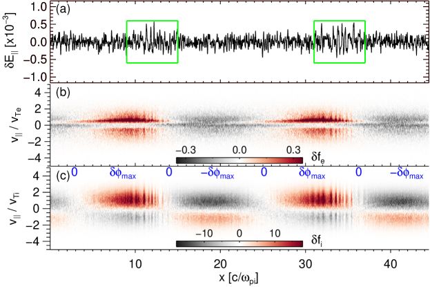
Figure 4: TDSs and phase space portraits in Simulation 1. This snapshot is taken at $t=100\,\omega_{ci}^{-1}$. (a) The parallel electric field. The green boxes mark the TDS locations. Hereafter in our PIC simulations, the electric field has the dimension $\frac{m_{e}c^{2}}{e\cdot c/\omega_{pe}}$. (b) The perturbed electron phase space density $\delta f_{e}$. (c) The perturbed ion phase space density $\delta f_{i}$. At the top of this panel, the phase of the potential field is annotated by blue text.

Figure 5: The localized electron velocity distribution function. This distribution is obtained by averaging the perturbed electron phase space density $\delta f_{e}$ in Figure 4 between $x\omega_{pi}/c=9$ and $x\omega_{pi}/c=11$. The two vertical dashed lines indicate the extent of the separatrix around the trapping island, which separates resonant electrons from nonresonant electrons.

Outside of the trapping island, the electrons are nonresonant and thus can be interpreted using

$$\delta f_{e}=\frac{1}{\frac{\omega_{0}}{k_{0\parallel}}-v_{\parallel}}\frac{e\delta\phi}{m_{e}}\frac{\partial f_{0e}}{\partial v_{\parallel}},$$ (11)

which is on an equal footing with Equation (10) for the nonresonant ion response. With the use of Equation (11), it is straightforward to demonstrate that a positive (negative) perturbation of electron phase space density $\delta f_{e}>0$ ($\delta f_{e}<0$) is produced in the phase of $\delta\phi>0$ ($\delta\phi<0$), as shown in Figure 4(b).

Electron beams driven by the kinetic Alfvén wave excite localized bursts of TDSs, appearing as bipolar electric field structures [Figure 4(a)]. The ratio of the parallel electric field amplitude of TDSs to that of the kinetic Alfvén wave is about $17$. These TDSs occur in the phase of $\delta E_{\parallel}>0$ (or $\partial\delta\phi/\partial x<0$). The exact occurrence phase of TDSs may depend on the cumulative growth rate $\int^{t}\gamma dt^{\prime}$ of beam instability over a certain time period, since the signal-to-noise ratio is modulated by $e^{{\int^{t}\gamma dt^{\prime}}}$. These TDSs are identified as nonlinear electron acoustic-mode [Holloway  Dorning (1991), Valentini . (2006), Anderegg . (2009)], which does not require the simultaneous presence of a cold electron component and a hot electron component as the usual electron acoustic-mode [Gary (1993)]. Instead, it survives undamped on the distribution of trapped electrons [Holloway  Dorning (1991)]. In the space environment, the existence of kinetic Alfvén waves of finite amplitude indicates that a plateau of finite width on the electron distribution function has to be created, otherwise kinetic Alfvén waves would be damped out. As a result, TDSs survive in the space enviroment because their phase velocities are located within this plateau.

The electric field perturbation of TDSs is largely along the $\mathbf{k}$ direction (i.e., the longitudinal electric field $\delta E_{L}$). To analyze the TDS properties, we show the spatiotemporal evolution of $\delta E_{L}$ and its Fourier spectra in Figures 6 and 7, respectively. TDSs propagate at a slightly larger phase velocity than the kinetic Alfvén wave [Figures 6 and 7(b)]. The spiky electric field of TDSs has the signature of broadband spectrum [Figures 7]. Using the range of TDS wavenumbers in the spectrum, we can estimate the spatial scales of TDSs as $25-50\lambda_{D}$. Due to the modest spatial bunching of trapped electrons, a weak second harmonic of the fundamental kinetic Alfvén wave is also generated [Figure 7(a)].

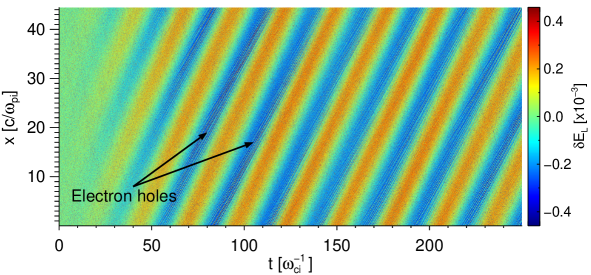
Figure 6: The spatiotemporal evolution of the longitudinal electric field $\delta E_{L}$ in Simulation 1. $\delta E_{L}$ is the projection of total electric field along the $\mathbf{k}$ direction. The phase and amplitude of $\delta E_{L}$ is color-coded.

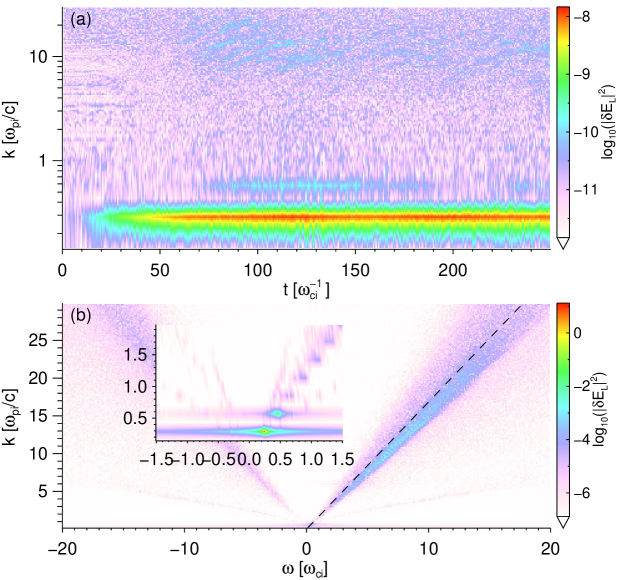
Figure 7: The Fourier spectra of the longitudinal electric field $\delta E_{L}$ in Simulation 1. (a) The temporal evolution of the wavenumber spectrum of $\delta E_{L}$. The wavenumber spectrum is obtained by Fourier-transforming the spatiotemporal pattern of $\delta E_{L}$ in space. The wavenumber of the fundamental kinetic Alfvén wave is $0.28\omega_{pi}/c$. The wavenumber of TDS is in the range $10$ - $20\,\omega_{pi}/c$. (b) The frequency-wavenumber diagram of $\delta E_{L}$. The reciprocal of the slope of the dashed line represents the phase velocity of the kinetic Alfvén wave. The inset plot zooms in on the fundamental kinetic Alfvén wave and its harmonics. We note that the weak signals propagating at $v=-v_{A}$ are likely caused by part of the resonant island extending to $v=-v_{A}$ as shown in Figure 5.

The excitation of TDSs is a manifestation of beam instabilities driven by the kinetic Alfvén wave. The majority of wave energy, however, is deposited into thermal electrons through nonlinear Landau resonance. Figure 8 shows how the final electron distribution has deviated from the initial Maxwellian. Around the Landau resonant velocity $v_{A}$, a region of high phase space density moves from $v_{\parallel}<v_{A}$ to $v_{\parallel}>v_{A}$ and a region of low phase space density moves from $v_{\parallel}>v_{A}$ to $v_{\parallel}<v_{A}$ via nonlinear phase trapping. This results in a net increase in the kinetic energy of the resonant electrons and a consequent damping of the kinetic Alfvén wave. Again, the estimated half width of the trapping region using Equation (6), $\Delta v_{tr}/v_{Te}=0.55$, is consistent with that shown in Figure 8(c).

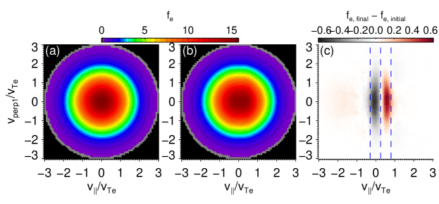
Figure 8: The thermal electron heating in Simulation 1. The density distribution in this figure has been averaged over the spatial domain. (a) The initial Maxwellian distribution. (b) The distribution at the end of the simulation. (c) The difference between the final and initial distribution functions. The three dashed lines from left to right stand for $v_{\parallel}=v_{A}-\Delta v_{tr}$, $v_{\parallel}=v_{A}$ and $v_{\parallel}=v_{A}+\Delta v_{tr}$, respectively.

3.3 Strong nonlinear Landau resonant interaction

In the second simulation, the wave magnetic mirror force is much smaller than the parallel electric force. The resulting half width of the trapping island is $\Delta v_{tr}/v_{Te}=1$, where we have used Equation (6) with the input $\delta B_{z}/B_{0}=0.004$ (obtained from the simulation) and $F_{zb}/F_{ze}=0.008$ (derived from the linear kinetic theory). For comparison, $\Delta v_{tr}/v_{Te}$ is about $0.55$ in the first simulation. Thus we would expect a stronger beam instability and potentially different characteristics of TDSs in the present case. Below we emphasize the differences between the first and second simulations.

The expectation of a strong beam instability is confirmed by the electron phase space plot [Figure 9(b)]. Spatially modulated, prominent electron beams are driven by the parallel electric field of the kinetic Alfvén wave inside the trapping island ($v_{A}-\Delta v_{tr}<v_{\parallel}<v_{A}+\Delta v_{tr}$). Solitary electric field structures are generated by these unstable beams. Several phase space holes are clearly identified in Figures 9(a) and 9(b). The ratio of the parallel electric field amplitude of TDSs to that of the kinetic Alfvén wave is about $10$. The phase space holes propagate at the local beam velocity, which is larger than $v_{A}$ [Figures 9(b) and 11(b)]. As a consequence, the phase space holes overtake the phase fronts of the kinetic Alfvén wave [Figure 10]. In addition, double layers are seen to form in the phase of maximum $\delta E_{\parallel}$, where the phase of $\delta E_{\parallel}$ is inferred from $\delta f_{i}$ using the technique in Section 3.2. The beam electrons are slowed down by the double layers and accumulate at the high potential sides of the double layers [Figure 9(b)], which eventually leads to the dissipation of double layers [Figure 10]. Finally, in comparison with the first simulation, more harmonics of the kinetic Alfvén wave are generated due to the nonlinear phase trapping of electrons [Figures 10 and 11].

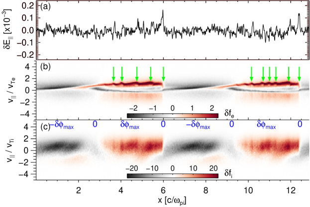
Figure 9: TDSs and phase space portraits in Simulation 2. This snapshot is taken at $t=61\,\omega_{ci}^{-1}$. (a) The parallel electric field. (b) The perturbed phase space density of electrons. Phase space structures in association with solitary electric fields are identified using arrows. Two of the arrows point to double layers at $x=6.0\,\,\text{and}\,\,12.5\,c/\omega_{pi}$. Other arrows point to phase space holes. (c) The perturbed phase space density of ions. The phase of potential field $\delta\phi$ is annotated by blue text.

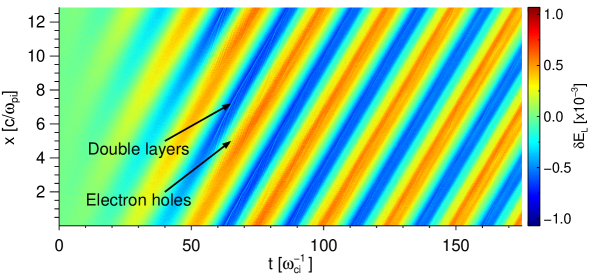
Figure 10: The spatiotemporal evolution of the longitudinal electric field $\delta E_{L}$ in Simulation 2. As indicated by the two arrows, phase space holes and double layers are embedded in the large scale kinetic Alfvén wave. The kinetic Alfvén wave field is distorted by its higher harmonics.

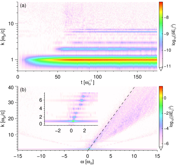
Figure 11: The Fourier spectra of the longitudinal electric field $\delta E_{L}$ in Simulation 2. (a) The temporal evolution of the wavenumber spectrum of $\delta E_{L}$. The wavenumber of the fundamental kinetic Alfvén wave is $0.98\omega_{pi}/c$. Higher harmonics of the kinetic Alfvén wave occur consecutively in time. TDSs start to be excited in the interval $50<t\omega_{ci}<100$ and are mainly located in the wavenumber range $10$ - $30\,\omega_{pi}/c$. (b) The frequency-wavenumber diagram of $\delta E_{L}$. Notably, the propagation velocity of TDSs is greater than that of the kinetic Alfvén wave, whereas the harmonics of the kinetic Alfvén wave propagate at the same velocity as the fundamental mode. The inset plot zooms in on the fundamental kinetic Alfvén wave and its harmonics.

Thermal electrons in the present simulation are more strongly heated through nonlinear Landau resonance than the first simulation. This produces an elongated electron distribution in the parallel velocity, known as the flat-top distribution [Figure 12]. Such a distribution has been previously obtained in coordinated observations and simulations [<]e.g.,¿damiano2018electron. The velocity range of the flat-top is consistent with the Landau resonance range, $v_{A}-\Delta v_{tr}<v_{\parallel}<v_{A}+\Delta v_{tr}$. Curiously, weak non-resonant electron heating is seen next to the Landau resonance at $v_{\parallel}<0$.

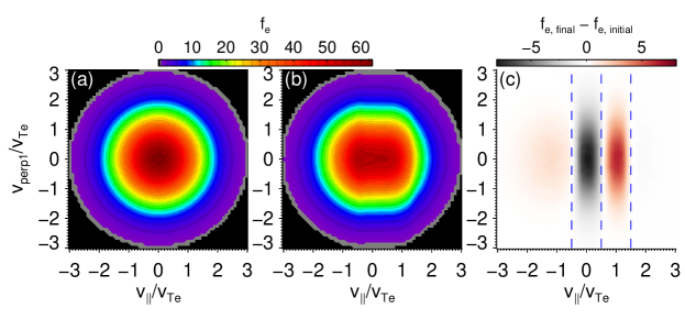
Figure 12: The thermal electron heating in Simulation 2. The density distribution has been averaged over the spatial domain. (a) The initial Maxwellian distribution. (b) The final flat-top distribution. (c) The difference between the final and initial distribution functions. The three dashed lines from left to right stand for $v_{\parallel}=v_{A}-\Delta v_{tr}$, $v_{\parallel}=v_{A}$ and $v_{\parallel}=v_{A}+\Delta v_{tr}$, respectively.

3.4 Critical condition for TDS excitation

As seen from the PIC simulations, the free energy source of TDSs is the trapped electron beam driven by the kinetic Alfvén wave. However, trapped electrons are subject to phase mixing [O’Neil (1965)] and thus the beam distribution is destroyed in a few trapping periods. Note that the phase mixing here refers to phase mixing of nonlinear Landau resonant electrons of different energies. How does the phase mixing rate of trapped electrons compare with the growth rate of the beam instability? To address this problem, we analyze the controlling factors of this process.

We separate the electron distribution into a Maxwellian $f_{0e}=\frac{1}{\sqrt{2\pi}v_{Te}}\exp\left(-\frac{v_{\parallel}^{2}}{2v_{Te}^{2}}\right)$ (by initialization) and a perturbed distribution $\delta f_{tr}$ (by trapped electrons) [see Figure 13]. The perturbed distribution comprises of a dip in the range $v_{A}-\Delta v_{tr}<v_{\parallel}<v_{A}$ and a bump in the range $v_{A}<v_{\parallel}<v_{A}+\Delta v_{tr}$, which is formally modeled as

$$\delta f_{tr}=\Delta f\cdot\sin\left(\pi\frac{v_{\parallel}-v_{A}}{\Delta v_{tr}}\right).$$ (12)

The magnitude of the perturbed distribution, $\Delta f$, is determined by

$$\Delta f=\frac{f_{0e}(v_{A}-\Delta v_{tr}/2)-f_{0e}(v_{A}+\Delta v_{tr}/2)}{2}.$$ (13)

Expanding $f_{0e}$ about $v_{\parallel}=v_{A}$ in Taylor series, we can rewrite $\Delta f$ as

$$\begin{split}\Delta f&=-\sum\limits_{n=0}^{\infty}\frac{1}{(2n+1)!}\left(\frac{\Delta v_{tr}}{2}\right)^{2n+1}f_{0e}^{(2n+1)}(v_{A})\\ &=\sum\limits_{n=0}^{\infty}\frac{H_{2n+1}\left(\frac{v_{A}}{\sqrt{2}v_{Te}}\right)}{(2n+1)!}\left(\frac{\Delta v_{tr}}{2\sqrt{2}v_{Te}}\right)^{2n+1}f_{0e}(v_{A}),\end{split}$$ (14)

where even terms in the Taylor series are canceled out and the Hermite Polynomial $H_{2n+1}$ is used for calculating derivatives of the Maxwellian distribution [Weber  Arfken (2003)].

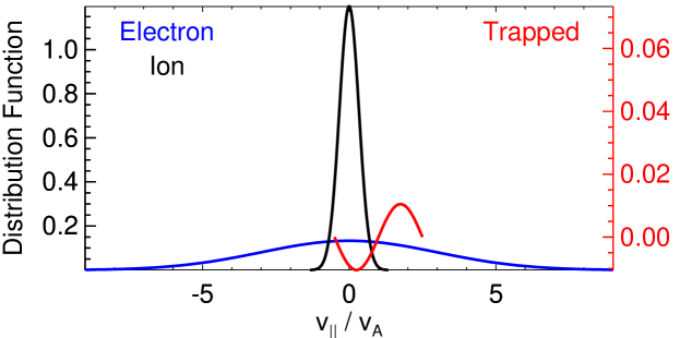
Figure 13: Sketch of distribution functions. The black line represents the ion Maxwellian distribution $f_{0i}$. The electron distribution is separated into an equilibrium part (blue; the Maxwellian distribution $f_{0e}$) and a perturbed part [red; $\delta f_{tr}$ in Equation (12)]. The perturbed part is induced by trapped electrons, the scale of which is shown by the vertical axis on the right.

The growth rate of the beam instability contributed by the trapped electrons can be written as [O’Neil  Malmberg (1968)]

$$\begin{split}\frac{\gamma_{tr}}{k_{\parallel}v_{Te}}&=\frac{\pi}{2}\frac{\omega}{k_{\parallel}v_{Te}}\frac{\omega_{pe}^{2}}{k_{\parallel}^{2}}\left(\frac{\partial}{\partial v_{\parallel}}\delta f_{tr}\right)_{v_{\parallel}=\omega/k_{\parallel}}\\ &\lesssim\frac{\pi}{2}\frac{\omega}{k_{\parallel}v_{Te}}\frac{\omega_{pe}^{2}}{k_{\parallel}^{2}}\left(\frac{\partial}{\partial v_{\parallel}}\delta f_{tr}\right)_{v_{\parallel}=v_{A}}\\ &=\frac{\pi}{2}\frac{\omega}{k_{\parallel}v_{Te}}\frac{1}{k_{\parallel}^{2}\lambda_{D}^{2}}\frac{\pi}{2\sqrt{2}}v_{Te}f_{0e}(v_{A})\\ &\times\sum\limits_{n=0}^{\infty}\frac{H_{2n+1}\left(\frac{v_{A}}{\sqrt{2}v_{Te}}\right)}{(2n+1)!}\left(\frac{e\delta\phi}{2T_{e}}\right)^{n},\end{split}$$ (15)

where $\omega/k_{\parallel}$ is the phase velocity of TDSs. The zeroth order term ($n=0$) of the beam growth rate does not depend on the wave amplitude $\delta\phi$ and always provides a positive growth rate [$H_{1}(v_{A}/\sqrt{2}v_{Te})>0$]. The next higher order term ($n=1$) linearly scales with $\delta\phi$, the sign of which depends on $H_{3}(v_{A}/\sqrt{2}v_{Te})$. For the range of interest (i.e., $v_{A}<v_{Te}$), we have $H_{3}(v_{A}/\sqrt{2}v_{Te})<0$, which means the beam growth rate decreases with the wave amplitude $\delta\phi$ in the regime of $v_{A}<v_{Te}$.

In the meantime, TDSs undergo Landau damping caused by $f_{0e}$ and $f_{0i}$ [Figure 13]. The ratio of electron Landau damping rate to ion Landau damping rate is

$$\frac{\gamma_{Le}}{\gamma_{Li}}=\frac{m_{i}}{m_{e}}\cdot\frac{v_{Ti}^{3}}{v_{Te}^{3}}e^{-\frac{v_{A}^{2}}{v_{Te}^{2}}+\frac{v_{A}^{2}}{v_{Ti}^{2}}}.$$ (16)

For typical values $T_{e}=300$ eV, $T_{i}=2000$ eV, $B_{0}=100$ nT, $n_{0}=1\,\text{cm}^{-3}$ around dipolarization fronts, we have $|\gamma_{Le}|\gg|\gamma_{Li}|$. Thus it suffices to consider only the electron Landau damping rate, i.e.,

$$\begin{split}\frac{\gamma_{Le}}{k_{\parallel}v_{Te}}&=\frac{\pi}{2}\frac{\omega}{k_{\parallel}v_{Te}}\frac{\omega_{pe}^{2}}{k_{\parallel}^{2}}f_{0e}^{\prime}(v_{A})\\ &=-\frac{\pi}{2}\frac{\omega}{k_{\parallel}v_{Te}}\frac{1}{k_{\parallel}^{2}\lambda_{D}^{2}}\frac{1}{\sqrt{2}}v_{Te}f_{0e}(v_{A})H_{1}\left(\frac{v_{A}}{\sqrt{2}v_{Te}}\right).\end{split}$$ (17)

The phase mixing rate of trapped electrons is characterized by the trapping frequency, i.e.,

$$\frac{\gamma_{\text{mixing}}}{k_{\parallel}v_{Te}}\sim\frac{\omega_{tr}}{k_{\parallel}v_{Te}}=\sqrt{\frac{e\delta\phi}{T_{e}}}\propto\sqrt{\delta\phi}.$$ (18)

The signal-to-noise ratio of TDSs can be estimated as $e^{(\gamma_{tr}+\gamma_{Le})\Delta t_{\text{mixing}}}$, where $\Delta t_{\text{mixing}}=1/\gamma_{\text{mixing}}$. Suppose that TDSs are observable after $N$ $e$-foldings. The critical condition for TDS excitation may be written as

$$\gamma_{tr}+\gamma_{Le}\geqslant N\gamma_{\text{mixing}}.$$ (19)

Plugging Equations (15), (17) and (18) into Equation (19), we explicitly obtain

$$\begin{split}\frac{\pi}{2\sqrt{2}}\frac{\omega}{k_{\parallel}v_{Te}}\frac{1}{k_{\parallel}^{2}\lambda_{D}^{2}}v_{Te}f_{0e}(v_{A})\left[\frac{\pi}{2}\sum\limits_{n=0}^{\infty}\frac{H_{2n+1}\left(\frac{v_{A}}{\sqrt{2}v_{Te}}\right)}{(2n+1)!}\left(\frac{e\delta\phi}{2T_{e}}\right)^{n}-H_{1}\left(\frac{v_{A}}{\sqrt{2}v_{Te}}\right)\right]\geqslant N\sqrt{\frac{e\delta\phi}{T_{e}}}.\end{split}$$ (20)

The TDS growth rate [left side of Inequality (20)] decreases with $\delta\phi$, whereas the phase mixing rate [right side of Inequality (20)] increases as $\sqrt{\delta\phi}$. This gives an upper bound of wave amplitude $\delta\phi_{c}$, beyond which the phase mixing rate exceeds the TDS growth rate and thus TDSs cannot be excited anymore. To find $\delta\phi_{c}$, we evaluate both sides of Inequality (20) as shown in Figure 14(a). In this procedure, we parameterize the TDS growth rate by $v_{A}/v_{Te}$. For a given normalized wave amplitude $e\delta\phi/T_{e}$, the TDS growth rate ($\gamma_{tr}+\gamma_{Le}$) increases with $v_{A}/v_{Te}$. For a given $v_{A}/v_{Te}$, the phase mixing rate exceeds the TDS growth rate at the critical amplitude $e\delta\phi_{c}/T_{e}$. We plot this critical amplitude $e\delta\phi_{c}/T_{e}$ as a function of $v_{A}/v_{Te}$ in Figure 14(b). For example, the critical amplitude is $e\delta\phi_{c}/T_{e}=0.078$ for $v_{A}/v_{Te}=0.25$ in Simulation 1, whereas the critical amplitude is $e\delta\phi_{c}/T_{e}=0.387$ for $v_{A}/v_{Te}=0.5$ in Simulation 2. Using Equation (2), we calculate the critical half width of the trapping island as $\Delta v_{tr,c}/v_{Te}=0.56$ for Simulation 1 and $\Delta v_{tr,c}/v_{Te}=1.24$ for Simulation 2. The measured half widths of the trapping island are below these critical values in each simulation. Additionally, we have confirmed that the excitation of TDSs is prohibited if the wave amplitude is above the critical value $\delta\phi_{c}$ in PIC simulations.

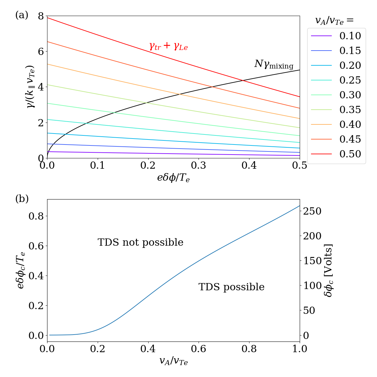
Figure 14: Critical condition for TDS excitation. (a) The comparison between the TDS growth rate and the phase mixing rate. In evaluating the TDS growth rate on the left side of Inequality (20), we use the typical TDS parameter $k_{\parallel}\lambda_{D}=0.1$, truncate the power series at $n=4$ (the resulting relative truncation error is less than $5\times 10^{-5}$), and parameterize the TDS growth rate by $v_{A}/v_{Te}$. The results are shown in rainbow-colored lines. In evaluating the phase mixing rate on the right side of Inequality (20), we take the number of e-folding as $N=7$ (i.e., the signal-to-noise ratio is $e^{7}\simeq 10^{3}$). The result is shown in the black line. For given values of $v_{A}/v_{Te}$ and $e\delta\phi/T_{e}$, if the phase mixing rate is greater than the TDS growth rate, excitation of TDSs is prohibited due to electron phase mixing. (b) The critical potential amplitude of kinetic Alfvén waves to drive TDSs. Beyond the critical potential amplitude $\delta\phi_{c}$, TDSs cannot be excited through electron trapping by kinetic Alfvén waves. The texts “TDS possible” and “TDS not possible” indicate the allowed and prohibited regions respectively in the parameter space for excitation of TDSs. To have a better comparison with spacecraft observations, the critical potential $\delta\phi_{c}$ is shown in the physical unit “volts” on the $y$ axis on the right for a typical electron temperature $T_{e}=300$ eV.

4 Conclusions

In this paper we have presented the excitation of TDSs through nonlinear Landau resonant interaction between kinetic Alfvén waves and thermal electrons. First, we show that the parallel electric field of the kinetic Alfvén wave is the primary driver of electron phase trapping. Second, we demonstrate that a spatially modulated beam distribution is formed by phase-trapped electrons and excites TDSs through the beam instability. Thermal electrons are heated by the kinetic Alfvén wave in the nonlinear trapping process. Third, we demonstrate that the TDS growth rate decreases with the wave potential $\delta\phi$ whereas the phase mixing rate scales with $\sqrt{\delta\phi}$. A critical condition for TDS excitation is thus derived [Equation (20)] and an upper bound of $\delta\phi$ is obtained [Figure 14].

Putting this work in the bigger context regarding the dissipation of the injection energy in the inner magnetosphere, a picture of energy cascading emerges as follows [Figure 15]: (1) The energy carried by the flow and the magnetic field of dipolarization fronts at macroscale is first converted to that of kinetic Alfvén waves and whistler waves; (2) These kinetic Alfvén waves and whistler waves then drive TDSs by accelerating electron beams locally through nonlinear Landau resonance; (3) In the meantime, kinetic Alfvén waves and whistler waves, together with TDSs, heat thermal electrons. In this way, energy cascades from dipolarization fronts at the macroscale to TDSs at the microscale, and is eventually deposited to electron thermal energy. Such a picture of energy cascading is being actively sought by combining global MHD simulations, test particle simulations and kinetic instability analysis to conquer the vast scale separations between dipolarization fronts and TDSs [<]e.g.,¿[]ukhorskiy2018microscopic, ukhorskiy2019kinetic.

Figure 15: Energy cascading from macroscopic dipolarization fronts down to microscopic TDSs. In characterizing the spatial scales of different objects, we use the following typical parameters around dipolarization fronts: the background magnetic field $50$ - $150$ nT; plasma density $0.1$ - $1\,\text{cm}^{-3}$; ion temperature $1000$ - $2000$ eV; electron temperature $300$ eV. “KAWs” is the acronym for kinetic Alfvén waves.

Appendix A Linearized Vlasov equation for the reduced particle distribution

We use the the linearized Vlasov equation to describe the nonresonant response of the particle distribution. This equation reads

$$\left(\frac{\partial}{\partial t}+\mathbf{v}\cdot\frac{\partial}{\partial\mathbf{x}}\right)\delta F_{s}=-\frac{q_{s}}{m_{s}}\left[\delta\mathbf{E}+\frac{\mathbf{v}\times(\delta\mathbf{B}+\mathbf{B}_{0})}{c}\right]\cdot\frac{\partial F_{0s}}{\partial\mathbf{v}},$$ (21)

where $\delta F_{s}(t,\mathbf{x},\mathbf{v})$ and $F_{0s}(\mathbf{v})$ are the perturbed and equilibrium parts of the distribution function of species $s$, respectively. We aim to rewrite the linearized Vlasov equation in terms of the reduced distribution functions

$$\delta f_{s} = \iint dv_{1}\,dv_{2}\,\delta F_{s}=\langle\delta F_{s}\rangle,$$ (22)

$$f_{0s} = \iint dv_{1}\,dv_{2}\,F_{0s}=\langle F_{0s}\rangle,$$ (23)

where $v_{1}$ and $v_{2}$ are the two orthogonal velocity components perpendicular to $\mathbf{B}_{0}=B_{0}\hat{\mathbf{x}}_{3}$, and the notation $\langle\cdot\rangle$ is short for the velocity space integral $\iint dv_{1}\,dv_{2}$. By integrating Equation (21) over $v_{1}$ and $v_{2}$, we obtain

$$\begin{split}&\left(\frac{\partial}{\partial t}+v_{3}\frac{\partial}{\partial x_{3}}\right)\delta f_{s}+\frac{\partial}{\partial x_{1}}\langle v_{1}\delta F_{s}\rangle+\frac{\partial}{\partial x_{2}}\langle v_{2}\delta F_{s}\rangle\\ =&-\frac{q_{s}}{m_{s}}\left[\delta E_{3}\frac{\partial}{\partial v_{3}}f_{0s}+\frac{\delta B_{2}}{c}\frac{\partial}{\partial v_{3}}\langle v_{1}F_{0s}\rangle-\frac{\delta B_{1}}{c}\frac{\partial}{\partial v_{3}}\langle v_{2}F_{0s}\rangle\right].\end{split}$$ (24)

Here the term with $\partial/\partial v_{1}$ has been integrated to zero, because the acceleration in front of $\partial/\partial v_{1}$ is irrelevant to $v_{1}$ and thus we can directly perform the integration $\int dv_{1}\,\partial F_{0s}/\partial v_{1}=0$. The same technique has also been applied to the term with $\partial/\partial v_{2}$. By using the property that $F_{0s}$ is a Maxwellian, we have $\langle v_{1}F_{0s}\rangle=0$ and $\langle v_{2}F_{0s}\rangle=0$. Furthermore, $\delta F_{s}$ is a function of $\sqrt{v_{1}^{2}+v_{2}^{2}}$ but not a function of the gyro-phase. The reason is that the cyclotron resonant velocity is much larger than the electron/ion thermal velocity in this case and virtually no particles are in cyclotron resonance with the kinetic Alfvén wave. This leads to $\langle v_{1}\delta F_{s}\rangle=0$ and $\langle v_{2}\delta F_{s}\rangle=0$. With the above considerations, Equation (24) can be simplified as

$$\left(\frac{\partial}{\partial t}+v_{3}\frac{\partial}{\partial x_{3}}\right)\delta f_{s}=-\frac{q_{s}\delta E_{3}}{m_{s}}\frac{\partial f_{0s}}{\partial v_{3}}.$$ (25)

This is the linearized Vlasov equation for the reduced particle distribution.