Space Telescope and Optical Reverberation Mapping Project. XIII. An Atlas of UV and X-ray Spectroscopic Signatures of the Disk Wind in NGC 5548

Abstract

The unusual behavior of the spectral lines of NGC5548 during the STORM campaign demonstrated a missing piece in the structure of AGNs. For a two-month period in the middle of the campaign, the spectral lines showed a deficit in flux and a reduced response to the variations of the UV continuum. This was the first time that this behavior was unequivocally observed in an AGN. Our previous papers explained this as being due to a variable disk-wind which acts as a shield and alters the SED. Here we use Cloudy to create an atlas of photoionization models for a variety of disk-winds to study their effects on the SED. We show that the winds have three different cases: Case 1 winds are transparent, fully ionized and have minimal effects on the intrinsic SED, although they can produce some line emission, especially He ii  or FeK$\alpha$. We propose thatthis is the situation in most of the AGNs. Case 2 winds have a He⁺⁺-He⁺ ionization-front, block part of the XUV continuum but transmit much of the Lyman continuum. They lead to the observed abnormal behavior. Case 3 winds have H⁺ ionization-front and block much of the Lyman continuum. The results show that the presence of the winds has important effects on the spectral lines of AGNs. They will thus have an effect on the measurements of the black hole mass and the geometry of the AGN. This atlas of spectral simulations can serve as a guide to future reverberation campaigns.

1 INTRODUCTION

Active galactic nuclei (AGNs) provide one of the best tools to trace the evolution of galaxies and to apply constraints on the structure of the cosmos. They are the compact central regions of massive galaxies and the most luminous objects in the universe. Because of their high luminosity, they are detectable at very high redshift. Their brightness results from the accretion of matter into a supermassive black hole (SMBH) at their center. A long-standing goal of AGN research has been to understand the mass and inner structure through gas flows in AGNs; clearly, accreted gas powers the AGN itself and outflows must interact with the surrounding galaxy, and the details of these interactions have implications for galaxy evolution. Unfortunately, the gas flows within the black hole radius of influence are largely unresolved, which complicates our attempt to understand their structure and interactions.

Reverberation mapping (RM) is the fundamental method for determining the inner structure and mass of AGNs by use of temporal variations as a tool to study the spatially unresolvable flows and structures. The continuum emission that originates in the accretion disk surrounding the black hole undergoes irregular flux variations. The broad emission-line fluxes change in response to these variations, but with a time delay due to the light-travel time between the accretion disk and the broad line region (BLR); measurement of these time delays is the fundamental goal that underlies the technique of reverberation mapping (BMcK82; Pet93). Similarly, changes in the intrinsic absorption features allow us to make inferences about changes in the AGN spectral energy distribution (SED) as well as the ionization state, temperature, and density of the absorbing gas, and other characteristics.

The Seyfert 1 galaxy NGC 5548 has been the target of many reverberation campaigns (see Pet02; DeRosa15, and references therein). In 2013, the “Anatomy” campaign (Kaastra14; Mehd15; Mehd16; Arav15; Ursini15; Gesu15; Whewell15; Ebrero16; Cappi16) monitored this object mainly using XMM-Newton   and the Neil Gehrels Swift Observatory, enhanced with data from the HST   Cosmic Origins Spectrograph (COS). One year later, the Space Telescope and Optical Reverberation Mapping program, or AGN STORM , began observing the object using Hubble Space Telescope , the Neil Gehrels Swift  Observatory, and the Chandra X-Ray Observatory (DeRosa15; Edelson15; Fau16; Goad16; Mathur17; Pei17; Starkey17; Deh19a; Kriss19; Horn20; Deh20).

The results from both campaigns found that NGC 5548 was in an unusual state: In 2013, the Anatomy campaign revealed that strong and persistent soft X-ray absorption was present. This was produced by an ionized outflow which we term the line-of-sight (LOS) obscurer. The obscurer is an outflowing stream of ionized gas with embedded colder, denser parts (Kaastra14), blocking a considerable amount of the soft X-ray emission and causing simultaneous deep, broad UV absorption troughs (Mehd15).

High cadence HST   spectroscopy performed by the AGN STORM project in 2014 found that the emission lines strongly decorrelated from the continuum for 70 of the 180 days of the campaign. In the words of the investigators, the emission lines “went on holiday”. This kind of decorrelation had never been commented on before. DeRosa15 present details about the observations, and Goad16 and Pei17 give quantitative measurements of the holiday observed in the emission lines (the emission-lines holiday).

Subsequent work found that high-ionization absorption lines had a similar holiday (Kriss19). Deh19a, hereafter D19a, showed that this was due to changes in the covering factor (CF) of the LOS obscurer, as verified by the Swift observations. Deh19b, hereafter D19b, proposed that the LOS obscurer originates in a disk wind so that it must extend down to the equator. Ionizing radiation produced by the accretion disk must pass through the base of this wind, which we term the equatorial obscurer, before striking the BLR. D19b showed that the BLR holiday can be produced by changes in the density or column density of the equatorial obscurer. Later, Deh20, hereafter D20, used the HST , XMM-Newton , and NuSTAR observations to propose a proper model for the equatorial obscurer, leading to a model for the disk wind itself.

Such disk winds are common although few studies of their emission and transmission properties have been made. A number of studies, including Murray95; le04; Shemmer15; Revalski18, have invoked translucent screens that block part of the ionizing radiation to explain different parts of the AGN phenomenon. This paper is a systematic study of the transmission and emission properties of such translucent screens.

In the following Section, we explore the disk wind and its properties. We begin with the LOS obscurer in NGC 5548 because this is well studied and modelled. In Section three, we investigate how the existence of winds with different parameters will affect the SED transmitted through the wind or the emission originating from the wind. We identify three distinct scenarios which depend on whether H, He, or He⁺ ionization fronts are present in the cloud. Section four is dedicated to setting limits to the global covering factor of the upper part of the disk wind and its resulting emission. It is followed by a discussion of the base of the wind and the emission lines produced by it.

2 THE DISK WIND

While this paper is motivated by the holiday observed in NGC 5548, we are not trying to model or analyze any specific observation. We examine several ways by which these kinds of winds could affect the SED emitted by the sources and cause a holiday. These results should apply to the family of AGNs. Our goal is to show that cloud shadowing can have a dramatic effect on the spectra, and it must be considered in all AGN studies.

2.1 The Obscurers

Figure 1 of D19b shows the geometry of NGC 5548 and includes the disk wind. We refer to the upper part of the wind as the LOS obscurer since it blocks much of the soft X-rays. The LOS obscurer can be directly observed and has a well-determined column density, soft X-ray absorption, and variable covering factor. This obscurer affects the absorption lines (D19a), however, it does not directly affect the emission lines. The LOS obscurer first appeared in 2011 (Kaastra14) and began to cover the central source. The portion of the source that is covered by the LOS obscurer varies with time (Mehd16). During the holiday, it covered $\sim 86\%$ of the X-ray source and $\sim 30\%$ of the UV source (Kaastra14).

The base of the wind, launched from the disk, is called the equatorial obscurer. This obscurer is the one which affects the BLR emission lines and produces the emission line holiday. There are no measurements of its column density or any other physical properties, but it is likely denser than the LOS obscurer and has a higher column density since it is closer to the accretion disk, where it was originally produced. D20 proposed physical properties for the translucent equatorial obscurer for which the wind has a constant optical depth to be located at the minimum threshold to produce a holiday (based on figure 4 of D19b). However, a wind from anywhere else within the Case 2 area of D19b figure 4, will still produce the holiday, but will have different properties.

The SED striking the BLR first passes through the equatorial obscurer and D19b argues that this filtering causes the emission-line holiday. This obscurer absorbs a great deal of the original SED, so its emission may be significant. Below we discuss this in more detail.

The hydrogen density and the ionization parameter of both obscurers are unknown. Regarding the LOS obscurer, Kaastra14 derived an ionization parameter of $\log\xi=-1.2\ \rm erg\ cm\ s^{-1}$, however, later Cappi16, found a much higher ionization parameter, $\log\xi=0.4-0.8\ \rm erg\ cm\ s^{-1}$. Recently Kriss19 suggested a still higher ionization parameter of $\log\xi=0.8-0.95\ \rm erg\ cm\ s^{-1}$.

We note that there are two different ionization parameters: $\xi$ and U, which have been used in various STORM papers. The ionization parameter $\xi$ is defined as (Kallman01):

$$\xi = (4\pi)^{2}\int_{1Ryd}^{1000Ryd}\frac{J_{\nu}\,d\nu}{n({\rm H})}=\frac{F_{\rm ion}}{n({\rm H})}$$ (1)

$$= \frac{L_{\rm ion}}{n({\rm H})r^{2}}\ {\left[{\rm erg\,cm\,s}^{-1}\right]}$$

while the ionization parameter U is dimensionless and is defined by:

$$\rm U=\frac{Q({\rm H})}{4\pi r^{2}n(H)c},$$ (2)

in which Q(H)=$\int_{1Ryd}^{\infty}\frac{L_{\nu}\,d\nu}{h\nu}$ is the total ionizing photon luminosity. For the unobscured SED of NGC 5548, $\log\ \rm U=\log\xi-1.6$.

As figure 3 of D19b shows, the SED can be dramatically affected when the hydrogen density gets more substantial. The situation may be the same if other parameters, like metallicity, change. This paper examines a range of obscurer parameters to check for observed properties and possible predictions.

2.2 The Covering Factors and Implications for Explaining the Holiday

Three different types of covering factors will enter in the following discussion. First, the line of sight covering factor, LOS CF. It is the fraction of the continuum source covered, as seen from our line of sight. This covering factor is directly measured through the hardness ratio estimations based on Swift observations (Mehd16). Second, the global covering factor, GCF, the fraction of the sky covered by a cloud, as seen from the central object (Wang12). This type of CF is not in our LOS, and it matters when we study the total emission luminosity of an obscurer emission-line holiday. Third, the ensemble covering factor, ECF. This covering factor accounts for the total portion of the source covered by all clouds in all directions. The ensemble global covering factor is typically 20$\%$ and can be determined from the equivalent width (EW) of emission lines (Osterbrock06).

D19a describes a physical model that explains the absorption-line holiday as a result of changes in the LOS CF of the obscurer. In this model, the SED passes through the LOS obscurer before striking the absorption cloud. There is a minimal transition in EUV and soft X-ray. However, the FUV part of the SED is almost not touched. High ionization species are affected by these changes in a way that the absorption-line holiday occurs. This explanation is only reliable for the case of a LOS obscurer and is consistent with 2013 Swift  observations of NGC 5548.

The equatorial obscurer shields the BLR, altering the SED striking it. The ECF of the BLR is unusually large,  50$\%$, in NGC 5548 (integrated cloud covering fraction; Korista00), so the global covering factor of the equatorial obscurer must also be this large to explain the BLR holiday (D19b). For this reason, a CF-based model cannot explain the emission-line holiday. The equatoria obscurer, which is much closer to the BH than the BLR and is likely to be the base of the wind, has instabilities in its mass-loss rate leading to variations in its hydrogen density. D19b explains that the variations of the hydrogen density of the equatorial obscurer can give rise to the emission-line holiday.

These different covering factors matter because they define the portion of the spectrum absorbed by the obscurer. This affects the ability to block the SED striking the outer clouds, and also determines the emission from the obscurer. Below we show how changes in the parameters of the obscurer affect the SED transmitted through it or emitted by it.

3 THE EFFECTS OF DIFFERENT PARAMETERS-GENERAL CONSIDERATIONS

As mentioned earlier, two obscurers affect the spectrum of NGC 5548: the LOS obscurer with its impact on intervening absorption lines, and the equatorial obscurer with its impact on the broad emission line clouds. These obscurers have many free parameters and variations of any of these parameters will change the transmitted SED. This section considers the effects of these parameters starting from a standard model of the LOS obscurer. This offers a good starting point since it is the one with direct measurements and modeling of its absorption properties. Surprisingly, there have been very few systematic explorations of the physical properties of absorbing gas and the effects of such absorbers on the SED transmitted through them (e.g. see Ferland82; Kraem99; le04.

3.1 A Typical Cloud

Mehd15 derived a standard or baseline model for the LOS obscurer in NGC 5548. Their model suggested that the obscurer blocked all of the SED between the FUV (13.6 eV) and the X-ray (1 keV). The complicated changes in the narrow absorption lines, where their degree of line-continuum correlation depends on ionization potential (Kriss19), suggests that a portion of the SED may be transmitted through the obscurer. The EUV and XUV portions of the transmitted SED are incident upon and ionize the UV absorbing cloud. This transmitted SED depends on the obscurer’s energy-dependent optical depth, which in turn depends on the the obscurer’s metallicity (Z), hydrogen number density n(H), and ionization parameter ($\xi$ or U).

Some of the physical properties of the LOS obscurer are known since we observe it in absorption, while no properties of the equatorial obscurer are observationally identified, although it is arguably more important since it changes the relative strength and response amplitude of the emission lines. D20 used a new approach to propose some parameters for the equatorial obscurer. The SED transmitted through or emitted by each of the obscurers is dependent on their column density, hydrogen density, ionization parameter (or distance from the source), and metallicity. Here we investigate this dependency by modeling different obscurers with different values for these parameters. We start with a typical cloud, assuming a density that is typical of the BLR, $n(\rm H)=10^{10}cm^{-3}$, and we adopt the intrinsic SED described in figure 3 of D19a. We assume solar abundances (photospheric), which is cloudy’s default value (Ferland17) unless otherwise specified. We start by keeping the optical depth at 1 keV constant at the value that was directly observed. This largely reproduces the obscured SED shown in Mehd15. Please note that the best related models assume there are in fact two separate LOS obscurers with different physical properties such as column density, ionization parameter, and covering factor.

3.2 Varying the Ionization Parameter

We predict transmitted and emitted SEDs by changing the ionization parameter ($\xi$) but keeping all other quantities constant. Changes in the ionization parameter are equivalent to changes in the luminosity of the source. Thus, this section also accounts for variations of the central source luminosity.

To keep the thickness of the cloud constant, we kept the optical depth constant. For all of the models, an outer cloud boundary was set so that the absorption optical depth at 1 keV is $\tau_{abs}\approx$1.9, consistent with that observed (figure 7 of Mehd15). These models do not necessarily illustrate the obscurers of NGC 5548 but show how sensitive the transmitted/emitted SEDs could be to the variations of the ionization parameter. We ran cloudy (Ferland17) for a grid of ionization parameters between -1.5 and 2 with steps as small as 0.025 dex. Results can be seen dynamically in an animation available as a supplement to this paper. Figure 1 shows examples of both the transmitted SED and the total emission from the obscurer for five different values of the ionization parameter $\xi$. Please note that in this paper, all the Figures which are labeled to be the emission from the obscurer are actually the total emission, which is the sum of the transmitted and reflected continua and lines and assume 100$\%$ covering factor. The attenuated incident continuum is also shown.

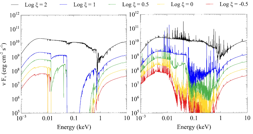
Figure 1: Left panel: The obscurer’s transmitted SED. As the lines show the transmitted SED is very sensitive to the ionization parameter in soft X-ray energies. Right panel: total emission(sum of the transmitted and reflected continua plus attenuated incident continuum) from the obscurer for different values of the ionization parameter. The attenuated incident continuum is included. The spectra represent $\log\xi=$2, 1, 0.5, 0, and $-0.5$ from top to bottom, and their total hydrogen column densities are $\sim 10^{22.7},10^{22.3},10^{22.1},10^{22},\rm and\ 10^{21.4}\rm cm^{-2}$, respectively. To create these models, the optical depth at 1 keV is kept constant and equal to the observed value. There is an animation associated with this Figure which dynamically illustrates the left panel of the Figure above. The animation shows how the transmitted SED responses to the variations of the ionization parameter for a range of $-1.5\ \rm erg\ \rm cm\ \rm s^{-1}\leq\xi\leq+2\ \rm erg\ \rm cm\ \rm s^{-1}$.The real time duration of the video is 6 seconds.

As the left panel of Figure 1 shows, the transmitted SED is spectacularly dependent on the value of the ionization parameter: clearly, the EUV part of the SED strongly depends on the ionization parameter while the XUV is always strongly attenuated unless we adopt a very high ionization parameter. For some ionization parameters, the EUV region is totally blocked, and for others, transmitted. When it comes to the emission from the obscurer, this dependency seems not to be as much as the transmitted SED, however, the higher the $\xi$ is the more emission is predicted.

Figure 1, left panel, shows three different styles of transmitted SED. These correspond to three different ionization states for hydrogen and helium within the obscurer. In order of decreasing ionization parameter, which lowers the ionization, increases the opacity, and decreases the transmission, these are:

• Case 1) Very high $\xi$ and ionization: Hydrogen is highly ionized, and the SED is fully transmitted. There is no ionization front in this case. The higher ionization means that all of the EUV and XUV passes through the cloud. There is not enough singly ionized helium to fully absorb the XUV. In other words, the obscurer is transparent.

• Case 2) Intermediate to high $\xi$ and ionization: Some of the EUV is transmitted, while little XUV light is transmitted. In this case, there is no He⁰-He⁺ionization front, but there is a He⁺ - He⁺⁺ ionization front. Enough atomic hydrogen is present to block much of the EUV, and the XUV is fully blocked by large amounts of singly ionized helium. In some samples of Case 2 (green line), there is a shallow H⁰ – H⁺ ionization front, however in other samples (blue), there is almost no hydrogen ionization front.

• Case3) Low $\xi$, low ionization: All EUV and XUV light is blocked. There is an H⁰ ionization front. There are significant amounts of atomic H that absorb much of the ionizing continuum. This is similar to the Mehd15 standard model of the obscurer. This is also the case for the LOS obscurer during the AGN STORM campaign and was assumed by Arav15 and D19a.

All the SEDs resulting from the full range of the adopted ionization parameters fall into one of these categories. Below we show that it does not matter which parameter of the obscurer is changing; the resulting transmitted SED will always be one of these three cases.

It is worth emphasizing that although we are motivated by the obscurers in NGC 5548 and we use this AGN as our point of reference, our discussion provides a framework for future AGN modeling. We study the effects of different obscurer properties on the transmitted SED. While all of the presented simulations use the properties of NGC 5548 and its obscurers as input, the approach should have a broader application.

3.2.1 A physical interpretation of three transmitted cases

We quantify the effects of these changes on the SED in Figure 2, which investigates variations of the ionization parameter, the independent axis, while the optical depth is kept constant. The upper panel gives the H⁰ column density. The lower panel shows the ratio of the intensity of the transmitted continuum at 399 Å  (EUV) relative to that at 1356 Å  (FUV). We selected these two wavelengths because they belong to two separate energy regions with very different responses to the changes in the ionization parameter, so they quantify the changes between the Cases described above. HST   measures the 1356 Å  point while we expect that a photoionized cloud is most affected by the 399 Å  point. This shows that the 399 Å  continuum is strongly extinguished for low ionization parameters, corresponding to Case 3. The abrupt change in the 399 Å  transmission and the atomic hydrogen column density occurs at the ionization parameter where there is no longer a hydrogen ionization front, and the cloud is highly ionized. This is the transition from Case 3 to Case 2. If the extinction changes due to a transition between Case 3 and 2, then the ionization state of the absorption cloud will not directly track the HST  continuum.

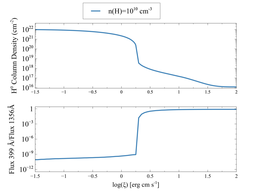
Figure 2: Top panel shows the variation of atomic hydrogen column density as the ionization parameter changes. The bottom panel shows the ratio of 399Å/1365Å as a function of the ionization parameter.

3.2.2 An upper limit for the ionization parameter

It is possible to calculate the upper limit of ionization parameter U (and so $\xi$) for which each of these cases could be possible. This will help to adjust the limit on the ionization parameter based on the model. Below we calculate three different maximum value ionization parameters for which a cloud could have ionization fronts and so modify the transmitted SED. We assume that the cloud has a column density of $\rm N(\rm H)=1.2\times 10^{22}\rm cm^{-2}$. We also assume that the nebula is optically thick with a temperature of $\rm T=10^{4}K$.

The transmitted continuum has to be opaque at the hydrogen edge to have an H⁰-H⁺ ionization front. This means that all the photons with energies more than 1 Rydberg are absorbed by the neutral hydrogen and an electron and H⁺ are produced (H⁰+$\gamma$ $\longrightarrow$H⁺+e ^-) also there is an equilibrium balance. Photoionization balance is the detailed balance between photoionization and recombination by electrons and ions (Osterbrock06):

$$\phi(\rm H)=n_{e}\alpha_{B}(H,T)n_{H^{+}}L_{Stromgren}\ \rm(photons\rm\ s^{-1}\rm cm^{-2})$$ (3)

$$=\rm n_{e}\alpha_{B}(H,T)N_{IF}(H^{+})\ \rm(photons\rm\ s^{-1}\rm cm^{-2}),$$

in which IF stands for the ionization front and L_Stromgren is the physical thickness of the Stromgren sphere (H II  region).

$$\Rightarrow\rm N_{IF}=\frac{\phi(\rm H)}{n_{e}\alpha_{B}(H,T)}$$ (4)

Since it is always the case that N${}_{\rm IF}<$N:

$$\frac{\phi(\rm H)}{\rm n_{e}\alpha_{B}(\rm H,T)}<1.2\times 10^{22}\rm cm^{-2}$$ (5)

and:

$$\phi(\rm H)=\rm U\ c\ n_{e}$$ (6)

$$\Rightarrow\frac{\rm Uc}{\alpha_{B}(\rm H,T)}<1.2\times 10^{22}\rm cm^{-2}$$ (7)

while, $\alpha_{B}(\rm H,10^{4}\hbox{K})=2.59\times 10^{-13}\rm cm^{3}s^{-1}$,

so for the assumed column density :

$$\Rightarrow\rm U<10^{-0.98}\rm$$ (8)

This is the upper limit in the hydrogen ionization parameter that ensures a hydrogen ionization front. We can always use the relationships explained in D19a to transform between U and $\xi$ (for the SED of NGC 5548: $\log\rm U\approx\log\xi-1.6$ ) .

The exact same discussion works for the He⁰-He⁺ ionization front, in which the equilibrium state is:

$$\phi(\rm He^{0})=n_{e}\alpha_{B}(He^{0},T)n_{He^{+}}L_{Stromgren}$$ (9)

$$=\rm n_{e}\alpha_{B}(He^{0},T)N_{IF}(He^{+})$$

We assume the cosmic abundance ratio of He/H to be almost 10%. This results in a helium column density of $\rm N(He^{+})=0.1\times N(\rm H)$, so to have a helium ionization front:

$$\phi(\rm He^{0})=n_{e}\alpha_{B}(He^{0},T)N_{IF}(H)\times 0.1$$ (10)

$$\frac{\phi(\rm H)}{\rm n_{e}}\times\frac{\phi(\rm He^{0})}{\phi(\rm H)}\times\frac{1}{\alpha_{B}(\rm He^{0},T)\times 0.1}=$$ (11)

$$\rm U\ c\times\frac{\phi(\rm He^{0})}{\phi(\rm H)}\times\frac{1}{\alpha_{B}(He^{0},T)\times 0.1}<1.2\times 10^{22},$$

in which $\alpha_{B}(\rm He^{0},10^{4}\hbox{K})=2.72\times 10^{-13}\hbox{cm}^{3}\hbox{s}^{-1}$.

For the adopted SED and an obscurer located at r $\approx 10^{18}$ cm (to be consistent with the LOS obscurer), we find:

$$\phi(\rm H)=2.27\times 10^{17}\rm cm^{-2}s^{-1}$$

$$\phi(\rm He^{0})=1.12\times 10^{17}\rm cm^{-2}s^{-1}$$

$$\phi(\rm He^{+})=4.22\times 10^{16}\rm cm^{-2}s^{-1}$$

These result in:

$$\Rightarrow\rm U<10^{-1.65}\rm$$ (12)

And similarly, to have a He⁺-He⁺⁺ ionization front:

$$\phi(\rm He^{+})=n_{e}\alpha_{B}(\rm He^{+},T)N_{IF}(He^{++})$$ (13)

for which $\rm N_{IF}(He^{++})\approx N_{IF}(He^{+})=0.1\times N(H)$ and $\alpha_{B}(\rm He^{+},10^{4}\hbox{K})=1.5\times 10^{-12}\hbox{cm}^{3}\hbox{s}^{-1}$, so:

$$\frac{\phi(\rm H)}{n_{e}}\times\frac{\phi(\rm He^{+})}{\phi(\rm H)}\times\frac{1}{\alpha_{B}(\rm He^{+},T)\times 0.1}=$$ (14)

$$\rm U\ c\times\frac{\phi(\rm He^{+})}{\phi(\rm H)}\times\frac{1}{\alpha_{B}(He^{+},T)\times 0.1}<1.2\times 10^{22}$$

$$\Rightarrow\rm U<10^{-0.48}\rm.$$ (15)

Table 1 summarizes the results. Please note that if we use a different location for the obscuring cloud, all the values for $\phi(\rm H)$, $\phi(\rm He^{0})$, and $\phi(\rm He^{+})$ will change accordingly and by the same scale. Thus, based on equations 11 and 14, the final results will stay unchanged.

Ionization Front	$\log\rm U_{\rm Max}$	$\log\xi_{\rm Max}$
H0-H+	-0.98	0.62
He0-He+	-1.65	-0.05
He+-He++	-0.48	1.12

Table 1: Upper limits for the ionization parameter to have various ionization fronts.

properly describe the recombination process at such densities. cloudy has such a model for one and two electron ions (section 3.2, Ferland17) but not for many-electron systems. CRM processes do not affect the X-ray opacity since that is produced by inner-shell electrons. The models presented here keep the total X-ray optical depth (at 1 keV) the same. As the density increases, H and He tend to become more ionized due to the increasing contribution from collisional (CRM model), and the EUV and XUV transmission increases. Because of the CRM, changing the density is very similar to changing the ionization parameter, due to due to the decreased efficiency in recombination. (Ferland17).

3.3 Varying the Column Density

The column density, N(H), is the number of atoms along the line of sight per unit area. In the simple case of a constant density n(H) cloud with thickness , $\rm N(\rm H)=n(\rm H)\delta R$. It is evident that a thicker or denser cloud would have a larger column density. To see how different values of the obscurer’s column density will affect the shape of the transmitted/emitted SED, we first multiplied optical depth of the LOS obscurer by four to make the cloud thicker than what was observed. Figure 3 shows the ionization structure versus depth for such a thick cloud, with an ionization parameter of $\log\xi$=-1.2 erg cm s^-1. In this Figure, the vertical dashed lines show three different depths that we will consider further. These are referred to as Case 1, Case 2, and Case 3 in the discussion below and we will show that they produce transmitted SEDs similar to those in Figure 1. These depths are chosen because, as the Figure shows, they correspond to different hydrogen and helium ionization states. The transmitted SED in each case reproduces one of the three cases discussed above and by D19b.

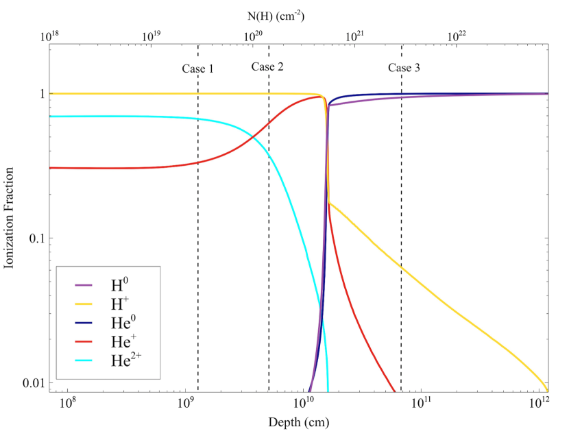
Figure 3: The ionization fraction of the noted ions as a function of the depth into the cloud (lower X-axis) in correspondence with the hydrogen column density (upper X-axis). The dashed lines show the depths corresponding to cases 1, 2, and 3, for assumptions of fixed gas density and incident ionizing photon flux. Figure 4 shows how the transmitted and emitted SEDs would be for these three different depths.

As Figure 3 shows, the ionization structure is very sensitive to the thickness of the cloud. The absorbing power of a cloud is proportional to the column density so larger column densities produce lower ionization as averaged over the cloud.

For the Case 1, both hydrogen and helium are fully ionized. As the red line shows, in Case 1, the amount of He⁺ is much smaller than H⁺ and He⁺⁺. There is not enough singly ionized helium to absorb the XUV. This means that the obscurer is transparent, and the intrinsic SED is fully transmitted. We propose that this is the case in most of AGNs: They DO have disk winds, but if the winds are in a transparent state no effects are observed. For Case 2, He⁺⁺ recombines to form He⁺ while H remains ionized. Both the transmitted SED and emitted He II photons will ionize any remaining H⁰. This is why the He⁺ zone is also an H⁺ zone. There is enough He⁺ to block a portion of the XUV although a significant fraction is transmitted. The presence of a He⁺⁺-He⁺ ionization front causes much of the 54 eV$<h\nu<$ 200 eV transmitted SED to be absorbed. This reproduces Case 2 discussed by D19b: the case in which the BLR holiday happens. Finally, for Case 3, photons with energies more than 13.6 eV are absorbed and atomic H and He forms. This reproduces Case 3 of D19b: a changing look quasar. In this case H⁺, He⁺ and He⁺⁺ ionization fronts are present.

Figure 4 shows the transmitted SED and the emission from the cloud for the three cases. The red line shows the SED for the Case 1 cloud. This SED is not strongly extinguished since there is no ionization front and hydrogen and helium remain ionized. In Case 2 and Case 3 hydrogen and helium ionization fronts occur, the SED is strongly absorbed and the diffuse continuum emission increases (Korista01; Korista19; Law18).

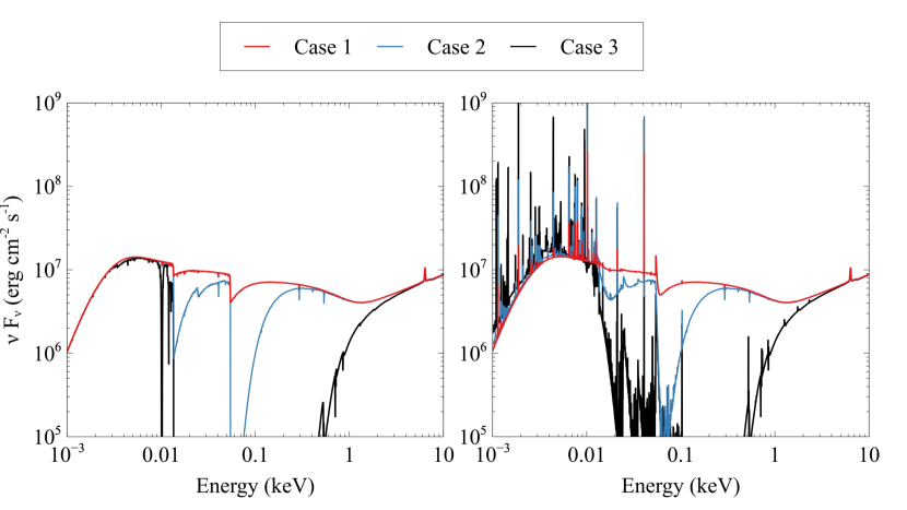
Figure 4: : Left panel: transmitted SED in different depths of a thick cloud. Right panel: total emission (sum of the transmitted and reflected continua plus attenuated incident continuum) from the obscurer for the same three cases.

3.4 Varying the Hydrogen Density

The hydrogen density of the LOS obscurer is poorly constrained. Here, we predict SEDs for different hydrogen densities while keeping the soft X-ray optical depth constant. We investigate the effects of changing density for two different values of the ionization parameter ($\log\xi$=0.5 erg cm s^-1 corresponding to Case 2, and $\log\xi$=-1.2 erg cm s ^-1 , corresponding to Case 3). Varying $\xi$ is equivalent to changing the distance between the obscurer and the accretion disk. Figure 5 shows the results.

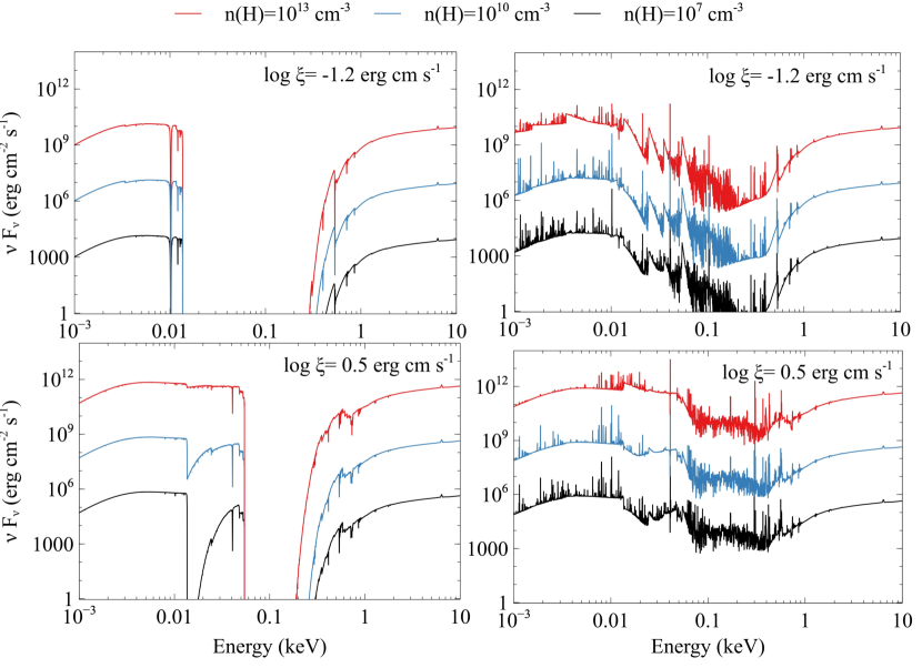
Figure 5: Changes in the SED for different values of the obscurer hydrogen density for two models of ionization parameters. Both upper panels have ionization parameter $\log\xi$=-1.2 erg cm s^-1. Upper left panel shows the results for the transmitted SED and the upper right shows the results for the total emission from the obscurer (sum of the transmitted and reflected continua plus attenuated incident continuum). Lower panels show the same concept for and ionization parameter $\log\xi$=0.5 erg cm s^-1.

In each of the four panels of the Figure 5, the ionization parameter is kept constant while the density varies. As noted earlier, simple homology relations suggest that clouds with similar ionization parameters, but different densities and flux of ionizing photons, should have the same ionization (Ferland03). The results for the lower ionization clouds are fairly similar. The results for the higher ionization parameter shown in the lower-left panel are surprising because the higher density clouds are more highly ionized and transparent. This is caused by the increasingly important role of collisional ionization from highly excited states in the high-radiation environment, as discussed earlier.

As the right panels of Figure 5 show, for energies in UV/optical regions, the obscurer also emits. This extra emission is stronger when the obscurer is denser. This excess of emission is mainly due to hydrogen radiative recombination in the optical and NIR and bremsstrahlung in the IR.

Figure 6 is similar to Figure 2. In this Figure, the upper panel shows the variations of the H⁰ column density as a function of the ionization parameter for three different hydrogen densities. As in Figure 2, the lower panel shows the ratio of the intensity of the transmitted continuum at 399 Å (EUV) relative to that at 1356 Å (FUV), this time for three different values of hydrogen density.

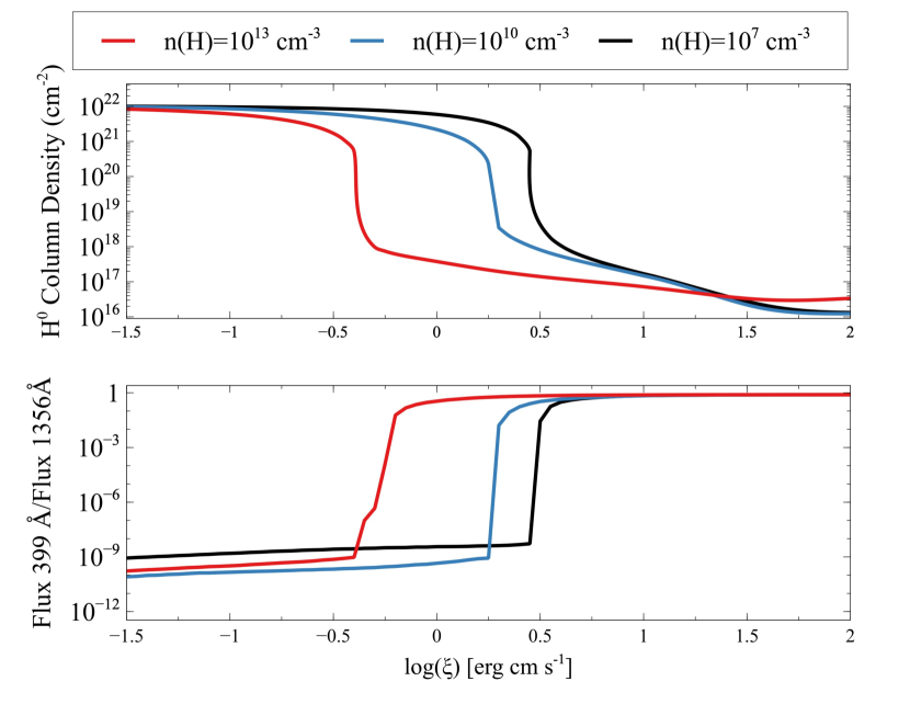
Figure 6: Top panel shows the variation of atomic hydrogen column density as the ionization parameter changes, for three different hydrogen densities. The bottom panel shows the ratio of 399Å/1365Å as a function of the ionization parameter for the same three hydrogen densities.

Please note that for the low densities, the CRM effects discussed earlier, are not important and simple photon conserving arguments hold. However, the CRM effects are considerable for higher densities and would affect the ionization front algorithm. This is the reason that we see different hydrogen ionization fronts for different values of the hydrogen density when the ionization parameter is $\log\xi$=0.5 erg cm s^-1.

3.5 Varying the Metallicity

We have assumed solar metallicity so far, and we next vary this. Since most soft X-ray absorption is produced by K-shell electrons of the heavy elements, one can expect that if we raise the metallicity by some factor, the hydrogen column density will fall by the same factor to keep the heavy element column density, and X-ray optical depth, the same. We checked this by modeling the transmitted and emitted SEDs for two very different values of the metallicity in two different models of ionization parameters.

The upper panels of Figure 7 show the transmitted SEDs (upper left) and the emission from the obscurer (upper right) for solar metallicity ($\rm Z_{\odot}$) and 10$\times$ $\rm Z_{\odot}$ for the ionization parameter $\log\xi$=-1.2 erg cm s^-1. Clearly, the transmitted SEDs of the upper left panel fall in Case 3 category. As both upper panels show, changing the metallicity does not profoundly affect the SED when we are in this case.

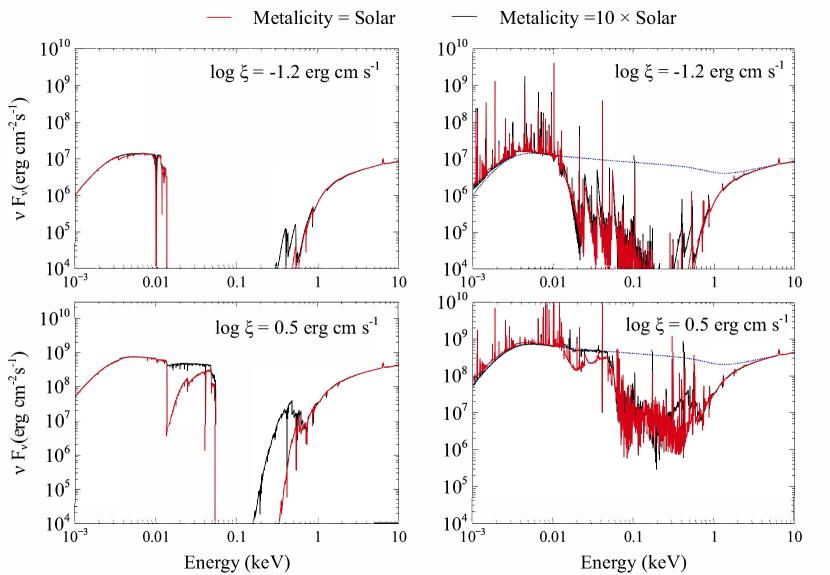
Figure 7: Changes in the SED for different values of the metallicity for two models of ionization parameters. Both upper panels have ionization parameter $\log\xi$=-1.2 erg cm s^-1. Upper left panel shows the results for the transmitted SED and the upper right shows the results for the total emission from the obscurer (sum of the transmitted and reflected continua plus attenuated incident continuum). Lower panels show the same concept for an ionization parameter $\log\xi$=0.5 erg cm s^-1.

The lower panels have an intermediate ionization parameter, $\log\xi$=0.5. Much of the soft X-ray extinction in the lower-left panel is produced by inner shell photoabsorption of the heavy elements. Although the 1 keV extinction, mainly produced by inner shells of O, C, is the same, the extinction around 200 – 400 eV changes significantly. The opacity in this range is mainly due to He and H (figure 10 of D19a) and little H⁰ or He⁰ is present. There is almost no hydrogen ionization front in the Z=10$\times$Z_⊙ case because the hydrogen column density is ten times smaller, as shown next. So, in this respect, the model behaves like Case 2 with no hydrogen ionization front.

Figure 8 is the equivalent to Figure 6, but for different metallicities. As expected, for the case with higher metallicity, the hydrogen column density is about 10 times smaller at low and high ionization parameters. However, there are much greater differences at intermediate $\xi$, around $\log\xi=\pm$0 erg cm s^-1. For these parameters, the locations of the hydrogen and helium ionization fronts, in the high-Z case, straddle the outer edge of the cloud and large changes in opacity occur.

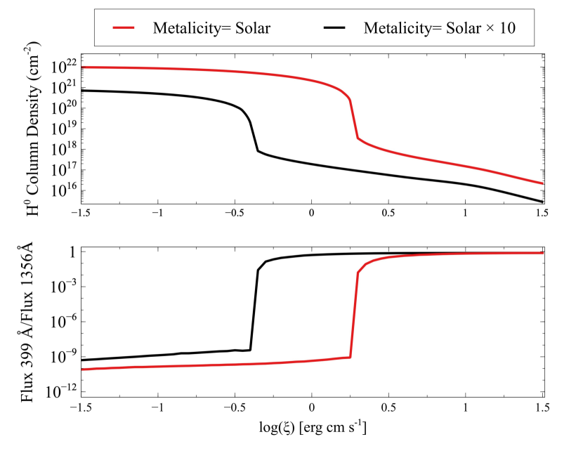
Figure 8: Top panel shows the variation of the obscurer atomic hydrogen column density as the ionization parameter changes for two different values of the metallicity. The bottom panel shows the ratio of the 399Å/1365Å transmitted continuum as a function of the ionization parameter.

3.6 Summary

All of the above discussions show that the SED filtered through an obscurer or reflected by it might change slightly or dramatically, depending on the obscurer’s properties. When the filtering happens, as in the case of NGC 5548, we could observe the original SED, the absorbed SED, and the reflected SED. Usually, it is not possible to directly measure the obscurer’s properties, however, by having the SEDs transmitted/reflected through the obscurer, one can find the characteristics of the obscurer itself, as demonstrated in D19b & D20a.

4 LIMITS ON THE OBSCURER: THE GLOBAL COVERING FACTOR

While the obscurer’s properties such as its hydrogen density and ionization parameter play a pivotal role in determination of the shape of the transmitted/reflected SED, we still need to know another characteristic of the obscurer, its global covering factor, to determine the geometry of the obscurer.

As seen from Earth, the obscurer in NGC 5548 absorbed a great deal of the energy emitted by the AGN since the ionizing photon luminosity fell from 2$\times$ 10⁴⁴ erg s^-1 to roughly 7.7$\times$10⁴³ erg s^-1 after obscuration (based on the SED modeling of Mehd16). The obscurer removed roughly 11.2$\times$ 10⁴³ erg s^-1, as seen by us if it fully covers the continuum source. Energy is conserved, so this light must be reradiated.

The total energy absorbed and emitted by the obscurer is determined by its global covering factor (explained in section 2.2), which is unknown. However, we do know that it persists for several orbital timescales (Kaastra14) so the geometry may be something like a symmetric cylinder covering 2$\pi$ around the equator (Figure1 of D19b). This suggests that the GCF may be significant. To check this, we derive the emission-line luminosities predicted by the LOS obscurer model to examine its spectrum and establish an upper limit on the LOS obscurer global covering factor.

4.1 The Luminosity of the Obscurer

Here we vary the distance between the obscurer and the central black hole (R_obs) to judge the magnitude of the effect on the obscurer’s emission lines. The most significant impact of doing this is to change the ionization parameter since it is proportional to R${}_{\rm obs}^{-2}$. The location of the wind in NGC 5548 is fairly well known. There is spectroscopic evidence showing the wind is located between the BLR and the source (i.e. R${}_{\rm obs}<10^{16}$cm). However, this is not the case for all AGNs, so it is informative to show how variations of the distance affect some of the wind’s properties to establish a diagnostic for other studies. Here we illustrate a novel method that uses limits to line intensities to establish bounds on the global covering factor and the location of the wind.

Figure 9 shows predicted emission-line luminosities for an obscurer that fully covers the continuum source, a GCF of 100$\%$ and has a hydrogen density of 10¹⁰ cm^-3. To create the model we considered a constant optical depth at 1 keV.

The predicted luminosities in Figure 9 can be compared with observations to obtain an upper limit to the obscurer’s GCF. The range of radii corresponds to changing the ionization parameter by a factor of 10⁸. The strongest spectral features are the Balmer continuum, Ly$\alpha$, C iv, and O VI. Of these, the Balmer continuum and Ly$\alpha$  have the least dependence on the unknown radius. We can compare the observed luminosity of Ly$\alpha$  with these predictions to set an upper limit on the obscurer’s GCF.

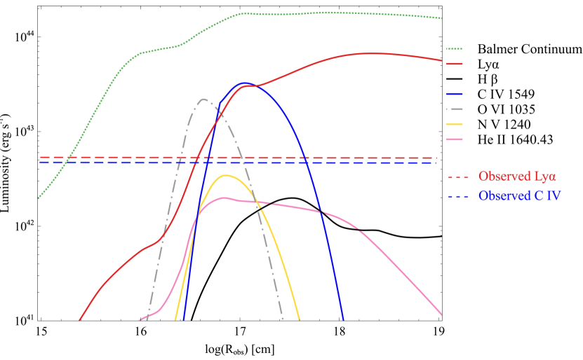
Figure 9: Changes in the luminosity of the emission features of the obscurer as the separation between the obscurer and the black hole varies between 10¹⁵ and 10¹⁹cm. The luminosities are predicted for full source coverage. The observed values refer to a combination of broad, medium broad, and very broad emission components observed by HST.

Table 1 of Kriss19 lists the UV emission lines in NGC 5548. Based on this information, the observed flux (broad+medium broad+very broad) for Ly$\alpha$  is 8.14$\times$10^-12 erg cm^-2 s^-1 (after correction for foreground Milky Way Galaxy extinction), and for the luminosity distance given by Mehd15, it has a luminosity of 5.36$\times$10⁴² erg s^-1. This value is shown with a red dashed line in Figure 9. The predicted Ly$\alpha$ luminosity can be either smaller or larger than this value. The Figure shows that we predict a Ly$\alpha$  luminosity of $\sim$ 5.46$\times$10⁴¹ erg s^-1 for R_obs= 10¹⁶ cm and full coverage. This value is almost 10 times smaller than that observed. It means that, based on the Ly$\alpha$  luminosity, if the obscurer is located at 10¹⁶ cm from the source, there is no need to constrain its GCF. If the same obscurer is located farther away, at R_obs= 10¹⁷ cm for instance, the predicted value is $\sim$ 2.85$\times$10⁴³ erg s^-1. This limits the obscurer global covering factor to be less than $\sim$ 19$\%$ . This shows that there is an interplay between the location of the obscurer, the emission line luminosities, and its global covering factor.

The C iv  line is much more model sensitive due to its dependence on the ionization parameter. Based on table 1 of Kriss19, the C iv  flux (broad+medium broad+very broad) is 7.17$\times$10^-12 erg cm^-2 s^-1 (after correction for foreground Milky Way Galaxy extinction), and this leads to a luminosity of 4.72$\times$10⁴² erg s^-1. Figure 9 shows that the predicted emission line luminosity varies by many orders of magnitude. For R_obs= 10¹⁶ cm, the predicted C iv  line luminosity, is much smaller than the observed value, as indicated by the blue dashed line. This means that GCF can be as large as 100$\%$. For larger radii, corresponding to smaller ionization parameters, the luminosity increases, reaching a maximum C iv  luminosity of 3.19$\times$10⁴³ erg s^-1, almost 7 times brighter than the observed value, requiring a covering factor less than one. We come away with the picture that the emission from the obscurer can be a contributor to the observed broad emission, and could, in fact, account for all of it, depending on the location of the obscurer. Next we investigate how the emission from the obscurer varies as a function of both its location and hydrogen density, for the three different cases discussed earlier.

5 EMISSION FROM THE WIND

D19b proposed that changes occuring in the base of the disk wind, the equatorial obscurer, explains the BLR holiday. This obscurer is located close to the central source and is assumed to absorb a significant amount of the SED striking the BLR. To conserve the energy, the obscurer must re-emit this energy. D20 showed that the equatorial obscurer produces its own emission lines and came up with a model in which the obscurer is not a dominant contributor to most of the strong emission lines, while it can be considered as the main He II and Fe K$\alpha$ emission source. In their model, the emission lines observed are indeed a combination of a broad core (produced in the BLR) and a very broad base (produced by the equatorial obscurer). Below we investigate various emission lines produced by the equatorial obscurer in each of the three cases that were discussed earlier.

5.1 Very broad emission lines

Figures 10 to 15 illustrate emission line equivalent widths for a variety of lines. Each of these Figures belongs to a single emission line and shows its behavior for the obscurer in Case 1, 2, or 3. To produce three different Cases, the optical depths are chosen such that each model of the obscurer falls in the middle of each region of figure 4 in D19b. This leads to a typical example of an obscurer for each case.

In each panel, the EW of the emission line is modeled as a function of both the flux of photons produced by the source ($\phi(\rm H)$) and the hydrogen density. To create these models, we used the SED of Mehd15 in cloudy (developer version), while we assumed photospheric solar abundances (Ferland17). We produced two-dimensional grids of photoionization models as we have done in D20. Each grid includes a range of total hydrogen density, 10${}^{10}\rm cm^{-3}<n(\rm H)<$ 10${}^{18}\rm cm^{-3}$, and a range of incident ionizing photon flux, 10²⁰ s^-1 cm${}^{-2}<\phi(\rm H)<$ 10${}^{24}\rm s^{-1}\rm cm^{-2}$. The flux of ionizing photons, the total ionizing photon luminosity Q(H), and the distance in light days are related by:

$$\phi(\rm H)=\frac{\rm Q(\rm H)}{4\pi r^{2}},$$ (16)

which indicates when the obscurer is closer to the source (smaller r), it will receive a larger amount of ionizing photon flux (larger $\phi(\rm H)$).

Considering the C iv  lag and based on Figure 4 of D20a, the C iv-forming region of the BLR has an incident ionizing photon flux of approximately 10${}^{21}\rm cm^{-2}\rm s^{-1}$, while the equatorial obscurer has an incident ionizing flux of almost 10${}^{22.5}\rm cm^{-2}\rm s^{-1}$, which means the equatorial obscurer is $\sim$6 times closer to the central source than a typical point in the BLR. Such an obscurer emits lines with a FWHM $\sim$4 time broader than the BLR if motions are virialized. As proposed by D20, the line EWs observed by HST   and other space telescopes are a combination of the broad emission from the BLR and the very broad emission from the equatorial obscurer.

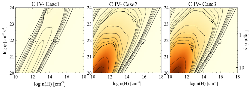
Figure 10: The EW of C iv emission line as a function of both the flux of hydrogen ionizing photons and the hydrogen density. Different panels show the variation of the EW for each of the discussed cases. The intervals between decades are logarithmic in 0.2 dex steps.

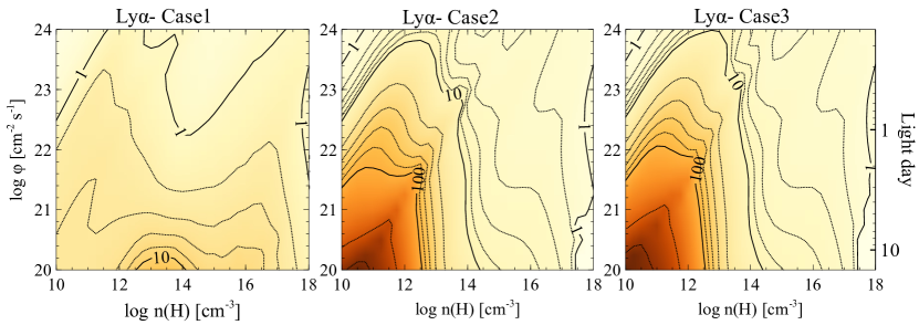
Figure 11: The EW of Ly$\alpha$  emission line as a function of both the flux of hydrogen ionizing photons and the hydrogen density. Different panels show the variation of the EW for each of the discussed cases.

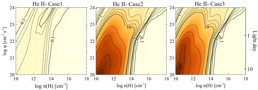
Figure 12: The EW of He ii  emission line as a function of both the flux of hydrogen ionizing photons and the hydrogen density. Different panels show the variation of the EW for each of the discussed cases.

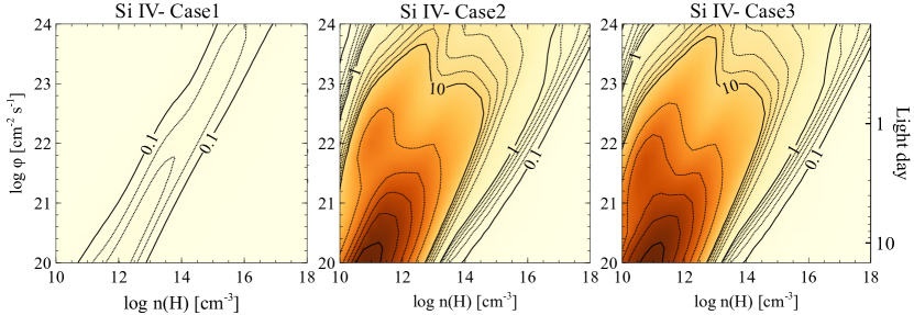
Figure 13: The EW of Si iv emission line as a function of both the flux of hydrogen ionizing photons and the hydrogen density. Different panels show the variation of the EW for each of the discussed cases.

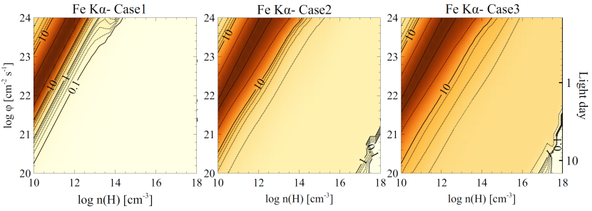
Figure 14: The EW of Fe K$\alpha$ emision line as a function of both the flux of hydrogen ionizing photons and the hydrogen density. Different panels show the variation of the EW for each of the discussed cases.

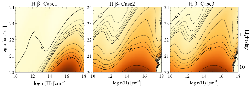
Figure 15: The EW of H$\beta$ emision line as a function of both the flux of hydrogen ionizing photons and the hydrogen density. Different panels show the variation of the EW for each of the discussed cases.

As Figures 10 to 13 show, when the wind is in a transparent state (Case 1), it emits very small amounts of C iv, He ii, Ly$\alpha$ and Si iv. In such a situation, almost all of the observed (broad+very broad) emission lines are mainly broad emission produced by the BLR and the equatorial obscurer has almost no contribution, regardless of where it is located or what its density is. This may be the case in most AGNs. However, when in Case 2 state, the contribution of the obscurer becomes significant. This means that by transformation from Case 1 to Case 2, there will be a change in the observed EW of the mentioned lines, which may lead to a holiday.

The predictions are different for Fe K$\alpha$ and H$\beta$  (Figures 14 and 15) emission lines. A transparent disk wind which is located close enough to the central source ($\phi(\rm H)>10^{21}\rm s^{-1}\rm cm^{-2}$) with a relatively low density ($\rm n(\rm H)~{}<10^{12}\rm cm^{-3}$) (Figure 14, Case 1, upper left corner) will produce Fe K$\alpha$ as much as a translucent disk wind. In this regime, the ions are too highly ionized to permit the Auger effect. Meanwhile, line photons are still affected by resonant scattering. There is no destruction mechanism so they can leave the disk. As a result, Fe K$\alpha$ XXV and XXVI will be emitted at 6.67 keV and 6.97 keV (Reynolds03). In this case, and based on the discussion of D20, both transparent and translucent disk winds can be a major contributor to the observed Fe K$\alpha$ emission. For NGC 5548, this confirms that the total amount of observed Fe K$\alpha$ will be almost constant before, during or after the holiday. Indeed, it does not matter which Case the wind state is in, it will always produce roughly the same amount of Fe K$\alpha$.

A transparent wind which is located far enough from the source ($\phi(\rm H)<10^{22}\rm s^{-1}\rm cm^{-2}$) with a large enough density ($n(\rm H)>10^{14}\rm cm^{-3}$) would produce almost as much H$\beta$ as produced by a translucent wind (Figure 15, Case 1, lower right corner). Table 6 of Pei17 reports that the flux of H$\beta$  had the smallest change (6$\%$) among the other strong emission lines (C iv, He ii, Ly$\alpha$  and Si iv). This is consistent with the behavior of H$\beta$  in our model, in which by transforming the wind from Case 1 (non-holiday) to Case 2 (holiday) the amount of H$\beta$  emitted by the equatorial obscurer is not affected dramatically, however, as we mentioned earlier, it is still affected enough to be consistent with the observed emission-line holiday. Depending on the optical depth, a translucent wind can be considered as Case 2 or Case 3. As Figures 10 to 15 show, for all of the emission lines, the behavior of a Case 2 obscurer is very similar to that of Case 3. D20 explained that a Case 3 wind could be a contributor to the changing-look phenomenon.

5.2 Summary

The equatorial obscurer is located close to the central source and, depending on whether it is transparent or translucent, it absorbs a small or large portion of the SED striking the BLR. The obscurer conserves energy by emitting very broad emission lines . For several of the strong UV emission lines, when the obscurer transforms from normal to a holiday phase, there is an increase in the very broad component, since the obscurer absorbs more energy than before. At the same time, the EWs of BLR broad emission components decrease due to receiving less energy from the source. The combination of these two phenomena leads to a decrease in the total (broad + very broad) observed emission line, i.e. a holiday. For some other lines, such as Fe K$\alpha$ and H$\beta$, the obscurer always emits almost the same amount of very broad emission line. This means its phase will not have any effects on absorbing that specific energy. As a result, it will not have a considerable effect on the BLR energy, and the total observed EWs of these lines seem almost constant during the transformation from normal to the holiday, and vice versa.

6 DISCUSSION: THE ROLE OF DISK WINDS IN THE AGN PHENOMENON

The STORM campaign showed that obscuration due to disk winds plays a major role in AGN variability. Obscurers are part of a disk wind so they can be common. These obscurers could cover a significant part of the continuum source and thus alter the SED striking the BLR or absorption clouds. As we show in Figures 1 and 5, there are conditions for which the obscurer is almost transparent, and so has no effect on the transmitted SED. We propose that this is the case in most AGNs in which no holiday is observed. If their effect is not observed, then it could be that they are in the transparent state (Case 1) which could be a result of low densities (D19b) or a high ionization parameter.

There are fewer UV reverberation campaigns than optical studies and holidays similar to NGC 5548 would be difficult to detect with optical data alone. In NGC 5548 the H$\beta$ EW did not change greatly during the holiday, (the flux deficit was only 6$\%$ (Pei17)) and our calculations predict that H$\beta$ does not change dramatically when the obscurer varies between Case 1 and Case 2. This makes it difficult to detect a holiday with optical data alone. Holidays may be more common than we now suspect.

When the obscurers are dense enough or highly ionized, they will emit. This emission could be a source of non-disk emission which will contribute to the observed broad emission. It is also possible that what is absorbed is radiated in FUV ranges, so is not detectable.

In such dense cases, the obscurer is removing a great deal of energy, and this can lead to the absence of BLR emission lines (D19b). This situation may provide an alternative cause of the changing-look phenomenon in AGNs. Right now, the only explanation for this phenomenon is that the source gets faint, so the BLR lines disappear. The obscurer can cause the changing look phenomenon in cases when the source is still bright, but the BLR lines are gone.

The STORM  campaign discovered an unexpected relationship between the ionizing SED and the response of the spectral lines. The extensive physical simulations carried out in this and previous papers quantifies how an intervening translucent screen can modify the SED and produce what HST   and XMM-Newton   observed for NGC 5548. This screen is most likely the inner portions of a disk wind so the HST spectral observations provide an indirect probe of a phenomenon that cannot be directly studied. The atlas of spectral simulations presented here will serve as a guide to future reverberation campaigns.