Study of Opportunistic Relaying and Jamming Based on Secrecy-Rate Maximization for Buffer-Aided Relay Systems

Abstract

In this paper, we investigate opportunistic relaying and jamming techniques and develop relay selection algorithms that maximize the secrecy rate for multiuser buffer-aided relay networks. We develop an approach to maximize the secrecy rate of relay systems that does not require the channel state information (CSI) of the eavesdroppers. We also devise relaying and jamming function selection (RJFS) algorithms to select multiple relay nodes as well as multiple jamming nodes to assist the transmission. In the proposed RJFS algorithms inter-relay interference cancellation (IC) is taken into account. IC is first performed to improve the transmission rate to legitimate users and then inter-relay IC is applied to amplify the jamming signal to the eavesdroppers and enhance the secrecy rate. With the buffer-aided relays the jamming signal can be stored at the relay nodes and a buffer-aided RJFS (BF-RJFS) algorithm is proposed. Greedy RJFS and BF-RJFS algorithms are then developed for relay selection with reduced complexity. Simulation results show that the proposed RJFS and BF-RJFS algorithms can achieve a higher secrecy rate performance than previously reported techniques even in the absence of CSI of the eavesdroppers.

I Introduction

The broadcast nature of wireless communications makes secure transmissions a very challenging problem. Security techniques implemented at the network layer rely on encryption keys which are nearly unbreakable. However, the computational cost of such encryption algorithms is extremely high. In order to reduce such cost novel security techniques at the physical layer have been developed. Physical-layer security was first conceived by Shannon in his landmark 1949 paper [1] using an information theoretic viewpoint, where the feasibility of physical-layer security has been theoretically discussed. Later on, Wyner proposed a wire-tap channel model that can achieve positive secrecy rates under the assumption that users have statistically better channels than those of the eavesdroppers[2]. Since then further research has been devoted to the wire-tap model in broadcast and multiple-antenna channels [3, 4, 5]. Techniques to enhance the secrecy of wireless systems such as artificial noise [6], beamforming [7] and relay techniques [8, 9] have also been extensively studied.

I-A Previous Work and Problems

Recently, the concept of physical-layer security with multiuser wireless networks has been thoroughly investigated and approaches based on transmit processing and relay techniques have drawn a great deal of attention [9, 10, 11, 12]. Transmit processing relies on intelligent design of precoding and signalling strategies to improve the secrecy rate performance. The use of relays [13] and the exploitation of spatial diversity can also enhance secrecy rates. Moreover, recent advances like buffer-aided relays have gained significant attention [14, 15, 16] as they can provide significant performance advantages over standard relays.

Buffer-aided relay systems with secure constraints have been investigated in half-duplex [14, 15, 17, 16] and full-duplex systems [18]. Opportunistic relay schemes have been examined with buffer-aided systems in [19, 20, 21]. In this context, inter-relay interference cancellation (IC) at relay nodes is a fundamental aspect in opportunistic relay schemes. In [19], IC has been combined with buffer-aided relays and power adjustment to mitigate inter-relay interference (IRI) and minimize the energy expenditure. Furthermore, in [20] a distributed joint relay-pair selection has been proposed with the aim of rate maximization in each time slot using a threshold to avoid increased relay-pair switching and CSI acquisition. In [21] and [22], a jammer selection algorithm and a joint relay and jammer selection technique have been investigated. The studies in [21] and [22] have shown that relaying contributes to a better transmission rate for legitimate users, whereas jamming can deteriorate the transmission to the eavesdropper. Therefore, relaying and jamming lead to an improvement in secrecy rate performance. However, opportunistic buffer-aided relay schemes with jamming techniques for improving physical layer security have not been examined so far.

I-B Contributions

In this work, we propose an opportunistic relaying and jamming scheme and develop relay selection algorithms for the downlink of multiuser single-antenna and multiple-input multiple-output (MIMO) buffer-aided relay networks that maximize the secrecy rate, which is a challenging task due to the difficulty to obtain CSI of the eavesdroppers. Preliminary results of the proposed techniques have been reported in [23], where relaying and jamming selection have been examined, and in [24], where relay selection based on the secrecy rate has been studied. Here, we devise a relay selection approach for effective secrecy rate (E-SR) maximization that does not require CSI of the eavesdroppers. The proposed relaying and jamming function selection (RJFS) algorithms select multiple relay nodes as well as multiple jamming nodes to help the transmission. We also present an opportunistic relaying and jamming scheme in which relaying or jamming is performed within the same set of relays at different time slots. In the proposed RJFS algorithms, IC is employed to improve the transmission rate to legitimate users and the residual interference is used to amplify the jamming signal to the eavesdroppers. We exploit buffer-aided relays to store the jamming signals at the relay nodes and devise a buffer-aided relaying and jamming function selection (BF-RJFS) algorithm. Greedy RJFS and BF-RJFS algorithms are also developed for relay selection with reduced complexity. Simulations show that the proposed RJFS and BF-RJFS algorithms can outperform previously reported techniques in the absence of CSI of the eavesdroppers. In addition, the greedy RJFS and BF-RJFS algorithms achieve a performance close to that of the exhaustive search-based RJFS and BF-RJFS algorithms, while requiring a much lower computational cost. The main contributions of this work are:

• The E-SR maximization approach that does not require CSI of the eavesdroppers is proposed.

• An opportunistic relaying and jamming scheme for single-antenna and MIMO buffer-aided relay systems.

• Novel RJFS algorithms that maximize the secrecy rate are developed for buffer-aided relay systems.

• Greedy RJFS and BF-RJFS algorithms are developed to reduce the computational complexity of exhaustive search-based RJFS and BF-RJFS algorithms.

• A secrecy rate analysis of the proposed RJFS algorithms.

This paper is organized as follows. In Section II, the system model and problem formulation are introduced. A review of relay selection techniques and a novel relay selection criterion without CSI to the eavesdroppers are included in Section III. The proposed RJFS and BF-RJFS algorithms are introduced in Section IV. In Section V a secrecy analysis is carried out. In Section VI, we present and discuss the simulation results. The conclusions are given in Section VII.

I-C Notation

Notation	Description
${\boldsymbol{A}}\in{\mathbb{C}}^{M\times N}$	denotes matrices of size ${M\times N}$
${\boldsymbol{a}}\in{\mathbb{C}}^{M\times 1}$	denotes column vectors of length $M$
$(\cdot)^{\ast}$, $(\cdot)^{T}$ and $(\cdot)^{H}$	represent conjugate, transpose,
	and conjugate transpose, respectively
$\boldsymbol{I}_{M}$	is an identity matrix with size $M$
$\rm diag\{\boldsymbol{a}\}$	is a diagonal matrix with the
	elements of $\boldsymbol{a}$ along its diagonal
$\mathcal{CN}(0,\sigma_{n}^{2})$	represents complex Gaussian
	random variables with independent
	and identically distributed ($i.i.d$)
	entries with mean $0$ and variance $\sigma_{n}^{2}$
$\log(\cdot)$	denotes the base-2 logarithm
$\|\boldsymbol{A}\|_{\rm F}$	is the Frobenius norm of ${\boldsymbol{A}}$
${\boldsymbol{H}}_{i}\in{\mathbb{C}}^{N_{i}\times N_{t}}$	is the channel matrix from the
	transmitter to the $i$th relay
$\boldsymbol{L}_{\rm state}\in{\mathbb{C}}^{S_{\rm total}N_{i}\times L}$	is the state matrix of the relays
${\boldsymbol{s}}^{(t)}\in{\mathbb{C}}^{MN_{i}\times 1}$	is the transmit signal at the source
${\boldsymbol{y}}_{i}^{(t)}\in{\mathbb{C}}^{N_{i}\times 1}$ and	refer to the received signals
${\boldsymbol{y}}_{r}^{(t)}\in{\mathbb{C}}^{N_{r}\times 1}$	at the relays and the destination
$\varGamma_{\rm{IC}-i}^{(t)}$, $\varGamma_{\rm{IC}-e}^{(t)}$	refer to SINR at the $i$th relay node, the
and $\varGamma_{\rm{IC}-r}^{(t)}$	$e$th eavesdropper and the $r$th receiver
$C_{s}$ and $R$	refer to secrecy capacity and rate
$\boldsymbol{\varOmega}^{r}$	refers to the set of $r$ selected relays
$\eta_{\rm LinkI}$ and $\eta_{\rm LinkII}$	refer to the selection thresholds
$P$	is the transmit power

II System Model and Problem Formulation

In this section, we introduce the multiuser MIMO buffer-aided relay system model along with details of the proposed opportunistic relaying and jamming scheme. The physical-layer security problem associated with the proposed opportunistic relaying and jamming scheme is then formulated.

II-A System Model

Figure 1: System model of a multiuser MIMO system with $M$ users, $N$ eavesdroppers and $S_{\rm total}$ relays.

Fig. 1 describes the downlink of an opportunistic multiuser MIMO relay system with $N_{t}$ antennas employed to transmit data streams aided by precoding to $M$ users in the presence of $N$ eavesdroppers. The system is equipped with a total of $S_{\rm total}$ relay nodes and a relay selection scheme that chooses $S$ out of $S_{\rm total}$ relay nodes. Each relay node is equipped with $N_{i}$ antennas and the buffer of each relay can store $L$ data packets. To show the states of the relays, we use the state matrix $\boldsymbol{L}_{\rm state}\in{\mathbb{C}}^{S_{\rm total}N_{i}\times L}$. Each column of the state matrix $\boldsymbol{L}_{\rm state}$ represents the signals stored in the buffers in one time slot. The buffer state matrix is initialized with zeros. Similarly to relay systems with two slots, the transmission can be divided into two parts: Link I and Link II. In Fig. 1, the solid lines represent the transmission of intended signals and the dashed lines denote the transmission of jamming signals. In Link I, the eavesdroppers try to obtain the signals transmitted from the source and the jamming signals will cause interference to the eavesdroppers. Furthermore, in Link II the eavesdroppers attempt to get the information from the selected relays. In this scenario, the jamming signals will be generated and transmitted by the relays. In such opportunistic scheme the relays can be selected to perform different functions in the same time slot. From Fig. 1 in both Link I and Link II, although the eavesdropper can accumulate the information received in both links, the relays selected to perform jamming will always transmit jamming signals to the eavesdroppers. Depending on the buffer size, the opportunistic scheme can be considered in two scenarios:

• Buffer size $L=1$: In the first time slot, only Link I is employed whereas in the second time slot Link II is used. As a result, there is no cooperation between Link I and Link II and the temporal advantage is unavailable in this scenario, which means this scheme is equivalent to a relay scheme without buffers.

• Buffer size $L>1$: The thresholds $\eta_{\rm LinkI}$ and $\eta_{\rm LinkII}$ that indicate the power allocation to the transmitter $\eta_{\rm LinkI}P$ or $\eta_{\rm LinkII}(2-P)$, where $P$ is the power, are calculated separately for Link I and Link II, which determines if the relays perform relaying or jamming.

  • If $\eta_{\rm LinkI}>\eta_{\rm LinkII}$, Link I is active. It indicates that the channels from the source to the relays can provide a better transmission environment. In this scenario, the jamming signals are generated independently at the relays, which are selected to perform the jamming function. The selection of the relays which perform the relaying function can be done according to different relay selection criteria. The jamming signal will also be stored at the buffers.

  • If $\eta_{\rm LinkI}\leq\eta_{\rm LinkII}$, Link II is active. It indicates that the channels from the relays to the users have better links. In this scenario, relays will forward the signals to the destination. The jamming signals in Link II are the stored jamming signals in Link I, which means that the jamming signals in Link II do not need to be generated in Link II.

If CSI remains unchanged or one link is always better than the other than the system will employ a counter, $\eta_{\rm L}$, compare it with a maximum value $\eta_{L_{\rm max}}$ and activate the link that has been inactive for $\eta_{L_{\rm max}}$ transmissions. The value $\eta_{L_{\rm max}}$ is set by the designer. In addition, the change of links makes it more difficult for the eavesdropper to obtain the pattern.

In this system, each relay node is equipped with $N_{i}$ antennas. To indicate when the relays are performing the jamming function, the relay antenna number is represented by $N_{k}$. For one relay we can have $N_{k}=N_{i}$. At the receiver side each user and each eavesdropper is equipped with $N_{r}$ and $N_{e}$ receive antennas. We also assume that the eavesdroppers do not jam the transmission and the data transmitted to each user, relay, jammer and eavesdropper experience a flat-fading MIMO channel. The quantities ${\boldsymbol{H}}_{i}\in{\mathbb{C}}^{N_{i}\times N_{t}}$ and ${\boldsymbol{H}}_{e}\in{\mathbb{C}}^{N_{e}\times N_{t}}$ denote the channel matrices of the ith relay and the eth eavesdropper, respectively. The quantities ${\boldsymbol{H}}_{ke}\in{\mathbb{C}}^{N_{e}\times N_{k}}$ and ${\boldsymbol{H}}_{kr}\in{\mathbb{C}}^{N_{r}\times N_{k}}$ denote the channel matrices of the kth relay to the eth eavesdropper and the kth relay to the rth user, respectively. The channel between the kth relay to the ith relay is represented by ${\boldsymbol{H}}_{ki}\in{\mathbb{C}}^{N_{i}\times N_{k}}$.

To support the transmission of data to $M$ users, the source is equipped with $N_{t}\geqslant N_{r}M$ antennas. The total number of antennas with $S$ relaying function nodes as well as $K$ jamming function nodes should satisfy $N_{i}S\geqslant N_{r}M$ and $N_{k}K\geqslant N_{r}M$, respectively. At the same time we assume that the total number of antennas of the eavesdroppers is $N_{e}N\geqslant N_{r}M$. In order to satisfy the precoding constraints [25], the number of $N_{r}M$ transmit antennas is used to transmit signals to $M$ users. The relays can estimate the channel from the jammers by assuming that there are pilots in the packet structure, that they know the jamming signals and that the eavesdroppers cannot decode the jammers. This is reasonable because the relays also perform jamming and therefore should know the jamming signals. Moreover, we also assume that CSI of the users can be obtained at the transmitter by feedback channels from the relays. Alternatively, advanced parameter estimation and relay techniques can be employed [26, 27, 28, 29, 30, 31, 32, 33, 34, 35, 36, 37, 38]. The vector ${\boldsymbol{s}}_{i}^{(t)}\in{\mathbb{C}}^{N_{i}\times 1}$ contains the data symbols of each user to be transmitted in time slot $t$. The transmit signal at the transmitter can be expressed as:

$${\boldsymbol{s}}^{(t)}={\left[{{\boldsymbol{s}}_{1}^{(t)}}^{T}\quad{{\boldsymbol{s}}_{2}^{(t)}}^{T}\quad\cdots\quad{{\boldsymbol{s}}_{M}^{(t)}}^{T}\right]}^{T}~{}\in{\mathbb{C}}^{MN_{i}\times 1}.$$ (1)

In previous works [39, 40, 41, 42, 43], precoding techniques have been applied to mitigate the interference among users. In this work, we adopt for simplicity linear zero-forcing precoding whose precoding matrix can be described by

$$\boldsymbol{U}^{(t)}={\boldsymbol{H}^{(t)}}^{H}({\boldsymbol{H}^{(t)}}{\boldsymbol{H}^{(t)}}^{H})^{-1}.$$ (2)

with ${\boldsymbol{U}}_{i}\in{\mathbb{C}}^{N_{t}\times N_{i}}$, the total precoding matrix can be expressed as

$${\boldsymbol{U}}^{(t)}=\left[{\boldsymbol{U}}_{1}^{(t)}\quad{\boldsymbol{U}}_{2}^{(t)}\quad\cdots\quad{\boldsymbol{U}}_{M}^{(t)}\right],$$ (3)

and the channel matrix to $S$ selected relays is given by

$${\boldsymbol{H}}^{(t)}={\left[{{\boldsymbol{H}}_{1}^{(t)}}^{T}\quad{{\boldsymbol{H}}_{2}^{(t)}}^{T}\quad\cdots\quad{{\boldsymbol{H}}_{S}^{(t)}}^{T}\right]}^{T}\in{\mathbb{C}}^{SN_{i}\times N_{t}}.$$ (4)

If the number of antennas equipped at each relay and each user are the same, the minimum required number of relays is ${\color[rgb]{0,0,0}S=M}$. The channels of the selected relays forwarding the signals to the $r$th user are described by

$${\boldsymbol{H}_{Kr}}^{(t)}={\left[{{\boldsymbol{H}}_{1r}^{(t)}}\quad{{\boldsymbol{H}}_{2r}^{(t)}}\quad\cdots\quad{{\boldsymbol{H}}_{Kr}^{(t)}}\right]}\in{\mathbb{C}}^{N_{r}\times KN_{k}}$$ (5)

and the channels from the relays to the users are described by

$${\boldsymbol{H}}_{M}^{(t)}={\left[{{\boldsymbol{H}}_{K1}^{(t)}}^{T}\quad{{\boldsymbol{H}}_{K2}^{(t)}}^{T}\quad\cdots\quad{{\boldsymbol{H}}_{KM}^{(t)}}^{T}\right]}^{T}\in{\mathbb{C}}^{MN_{r}\times KN_{k}}.$$ (6)

The selected relays also perform jamming for Link I’s transmission to the eavesdroppers, whereas the channels of the jammers to the $i$th relay are given by

$${\boldsymbol{H}_{Ki}}^{(t)}={\left[{{\boldsymbol{H}}_{1i}^{(t)}}\quad{{\boldsymbol{H}}_{2i}^{(t)}}\quad\cdots\quad{{\boldsymbol{H}}_{Ki}^{(t)}}\right]}\in{\mathbb{C}}^{N_{i}\times KN_{k}}.$$ (7)

In each link, if we assume that the total jamming signals are ${\boldsymbol{J}}=[{{\boldsymbol{j}}_{1}}^{T}\quad{{\boldsymbol{j}}_{2}}^{T}\quad\cdots\quad{{\boldsymbol{j}}_{K}}^{T}]^{T}$, the received signal ${\boldsymbol{y}}_{i}^{(t)}\in{\mathbb{C}}^{N_{i}\times 1}$ at each relay node can be expressed by

$${\boldsymbol{y}}_{i}^{(t)}={\boldsymbol{H}}_{i}\boldsymbol{U}_{i}{\boldsymbol{s}}_{i}^{(t)}+\sum_{j\neq i}{\boldsymbol{H}}_{i}\boldsymbol{U}_{j}{\boldsymbol{s}}_{j}^{(t)}+{\boldsymbol{H}}_{Ki}^{(t)}{\boldsymbol{J}}+\boldsymbol{n}_{i}$$ (8)

In (8), $\boldsymbol{n}_{i}\in\mathcal{CN}(0,\sigma^{2}_{n})$ and the superscript $pt$ designates the previous time slot when the signal is stored in the buffer at the relay nodes. The quantity $\sigma^{2}_{n}$ is the noise variance for the channel and ${\boldsymbol{H}}_{Ki}{\boldsymbol{J}}$ is regarded as the IRI among the $i$th relay and the $K$ jammers. The intended relays are selected according to different criteria, which will be explained later on. The received signals are expressed by ${\boldsymbol{y}}^{(pt)}=[{{\boldsymbol{y}}_{1}^{(pt_{1})}}^{T}\quad{{\boldsymbol{y}}_{2}^{(pt_{2})}}^{T}\quad\cdots\quad{{\boldsymbol{y}}_{S}^{(pt_{S})}}^{T}]^{T}$. The superscript $pt$ represents the time slot and due to the characteristics of buffer relay nodes, the values can be different for each relay node. According to the theorem in [19], IRI can be cancelled. The jammers are targeted towards the $e$th eavesdropper channel described by

$${\boldsymbol{H}_{Ke}}^{(t)}={\left[{{\boldsymbol{H}}_{1e}^{(t)}}\quad{{\boldsymbol{H}}_{2e}^{(t)}}\quad\cdots\quad{{\boldsymbol{H}}_{Ke}^{(t)}}\right]}\in{\mathbb{C}}^{N_{e}\times KN_{k}}$$ (9)

The received signal at the $e$th eavesdropper is then given by

$${\boldsymbol{y}}_{e}^{(t)}={\boldsymbol{H}}_{e}\boldsymbol{U}_{i}{\boldsymbol{s}}_{i}^{(t)}+\sum_{j\neq i}{\boldsymbol{H}}_{e}\boldsymbol{U}_{j}{\boldsymbol{s}}_{j}^{(t)}+{\boldsymbol{H}}_{Ke}^{(t)}{\boldsymbol{J}}+\boldsymbol{n}_{e}.$$ (10)

where $\boldsymbol{n}_{e}\in\mathcal{CN}(0,\sigma^{2}_{n})$ is the noise vector at the eavesdropper. For the eavesdropper, the term ${\boldsymbol{H}}_{Ke}^{(t)}{\boldsymbol{J}}$ acts as the jamming signal, which cannot be removed without CSI knowledge from the kth jammer to the eth eavesdropper.

If we assume that the transmitted signals from the relays to the users are expressed as ${\boldsymbol{r}}^{(t)}$, the received signal at the destination is given by

$${\boldsymbol{y}}_{r}^{(t)}={\boldsymbol{H}}_{M}{\color[rgb]{0,0,0}{\boldsymbol{r}}^{(t)}}+\boldsymbol{n}_{r}.$$ (11)

where $\boldsymbol{n}_{r}\in\mathcal{CN}(0,\sigma^{2}_{n})$ is the noise vector at the users.

In the existing IRI scenario based on (8) when the transmit signals $\boldsymbol{s}$ are statistically independent with unit average energy $\mathbb{E}[\boldsymbol{s}\boldsymbol{s}^{H}]=\boldsymbol{I}$, the SINR at relay node i $\varGamma_{\rm{IRI}-i}^{(t)}$ is expressed by

$$\varGamma_{\rm{IRI}-i}^{(t)}=\dfrac{{\gamma}_{S_{i},R_{i}}}{\varphi(k,i){\gamma}_{R_{K},R_{i}}+{\gamma}_{S_{j},R_{i}}+N_{i}},$$ (12)

where $\varphi(K,i)$ is the factor that describes the IC feasibility and $\boldsymbol{\gamma}_{m,n}$ represents the instantaneous received signal power for the links $m\longrightarrow n$ as described by

$${\gamma}_{S_{i},R_{i}}=\|\boldsymbol{H}_{i}\boldsymbol{U_{i}}\|_{\rm F},\quad{\gamma}_{S_{j},R_{i}}=\sum_{j\neq i}\|\boldsymbol{H}_{i}\boldsymbol{U_{j}}\|_{\rm F},$$ (13)

$${\gamma}_{R_{K},R_{i}}=\|\boldsymbol{H}_{Ki}{\color[rgb]{0,0,0}{\boldsymbol{y}}^{(pt)}}\|_{\rm F}.$$ (14)

The SINR at the $e$th eavesdropper node $\varGamma_{e}^{(t)}$ as well as the $r$th legitimate user $\varGamma_{r}^{(t)}$ is described by

$$\varGamma_{\rm{IRI}-e}^{(t)}=\dfrac{{\gamma}_{S_{i},E_{e}}}{{\gamma}_{R_{K},E_{e}}+{\gamma}_{S_{j},E_{e}}+N_{e}},$$ (15)

and

$$\varGamma_{\rm{IRI}-r}^{(t)}=\dfrac{{\gamma}_{R_{k},R_{r}}}{{\gamma}_{R_{K},R_{r}}+N_{r}},$$ (16)

where the terms in (15) and (16) are given by

$${\gamma}_{S_{i},E_{e}}=\|\boldsymbol{H}_{e}\boldsymbol{U_{i}}\|_{\rm F},\quad{\gamma}_{S_{j},E_{e}}=\sum_{j\neq i}\|\boldsymbol{H}_{e}\boldsymbol{U_{j}}\|_{\rm F},$$ (17)

$${\gamma}_{R_{K},E_{e}}=\|\boldsymbol{H}_{Ke}{\boldsymbol{J}}\|_{\rm F}$$ (18)

and

$${\gamma}_{R_{k},R_{r}}=\|\boldsymbol{H}_{kr}\boldsymbol{J}_{k}\|_{\rm F}.$$ (19)

$${\gamma}_{R_{K},R_{r}}=\|\boldsymbol{H}_{Kr}\boldsymbol{J}-\boldsymbol{H}_{kr}\boldsymbol{J}_{k}\|_{\rm F}.$$ (20)

Depending on the IRI cancelation (IC) at the relay nodes, two type of schemes can be applied. According to [19], if we assume $\mathbb{E}[\boldsymbol{s}\boldsymbol{s}^{H}]=\boldsymbol{I}$ and $\mathbb{E}[{\color[rgb]{0,0,0}{\boldsymbol{y}}^{(pt)}{{\boldsymbol{y}}^{(pt)}}^{H}}]=\boldsymbol{I}$, the feasibility of IC can be described by a factor $\varphi(K,i)$ which is described by

$$\varphi(K,i)=\begin{cases}0&\text{if $\det\Big{(}({\boldsymbol{H}_{i}\boldsymbol{H}_{i}^{H}+\boldsymbol{I}})^{-1}{\boldsymbol{H}_{Ki}\boldsymbol{H}_{Ki}^{H}}\Big{)}\geqslant\gamma_{0}$}\\ 1&\text{otherwise},\end{cases}$$ (21)

where $\varphi(K,i)=0$ means the interference can be cancelled from the received signal at the relays, whereas $\varphi(K,i)=1$ means IC should not be performed. The quantity $\gamma_{0}$ is the threshold that indicates the feasibility of IC, which is obtained by simulation. We assume that the channels from the relays, which perform jamming, are available at the transmitter.

In the IC scenario, interference mitigation can be performed at the relay nodes by setting $\varphi(K,i)=0$. The SINR expressions at the $i$th relay node, the $e$th eavesdropper and the $r$th receiver are respectively given by

$$\varGamma_{\rm{IC}-i}^{(t)}=\dfrac{{\gamma}_{S_{i},R_{i}}}{{\gamma}_{S_{j},R_{i}}+N_{i}},\quad\varGamma_{\rm{IC}-e}^{(t)}=\dfrac{{\gamma}_{S_{i},E_{e}}}{{\gamma}_{R_{K},E_{e}}+{\gamma}_{S_{j},E_{e}}+N_{e}}$$ (22)

and

$$\varGamma_{\rm{IC}-r}^{(t)}=\dfrac{{\gamma}_{R_{k},R_{r}}}{{\gamma}_{R_{K},R_{r}}+N_{r}}.$$ (23)

Alternative interference mitigation techniques can also be considered [44, 45, 46, 47, 48, 49, 50, 51, 52, 53, 53, 54] [32, 55, 56, 57, 58, 59, 60, 50, 61, 62, 63, 64, 65, 66, 34, 67] [68, 69, 70, 71, 31, 33, 46, 48, 72, 73, 74, 75, 76, 77, 78, 79, 80, 81, 82, 83, 35, 84] [85, 86, 43, 87, 88, 89, 30, 90, 64, 59, 91]

II-B Problem formulation

In this subsection, we describe the secrecy rate used in the literature to assess the performance of the proposed algorithms in physical-layer security systems and formulate the problem. The MIMO system secrecy capacity [4] is expressed by

$$\begin{split}C_{s}&=\max_{{\boldsymbol{Q}}_{s}\geq 0,\rm Tr({\boldsymbol{Q}}_{s})=E_{s}}\log(\det({\boldsymbol{I}}+{\boldsymbol{H}}_{ba}{\boldsymbol{Q}}_{s}{\boldsymbol{H}}_{ba}^{H}))\\ &\quad-\log(\det({\boldsymbol{I}}+{\boldsymbol{H}}_{ea}{\boldsymbol{Q}}_{s}{\boldsymbol{H}}_{ea}^{H})),\end{split}$$ (24)

where ${\boldsymbol{Q}}_{s}$ is the covariance matrix associated with the signal and ${\boldsymbol{H}}_{ba}$ and ${\boldsymbol{H}}_{ea}$ represent the links between the source to the users and the eavesdroppers, respectively. For relay systems [21], according to (8) and (11), with equal power $P$ allocated to the transmitter and the relays, the achievable rate of the users is given by

$$R_{r}=\log(\det({\boldsymbol{I}}+\boldsymbol{\Gamma}_{r}^{(t)}))$$ (25)

where $\boldsymbol{\Gamma}_{r}^{(t)}$ according to (16) is given by

$$\boldsymbol{\Gamma}_{r}^{(t)}=\frac{P}{\sum_{k=1}^{K}{N_{k}}}{\boldsymbol{H}}_{Kr}{\boldsymbol{H}}_{Kr}^{H}({\boldsymbol{I}}+\frac{P}{N_{t}}{\boldsymbol{H}}^{(pt)}{\boldsymbol{U}^{pt}}{\boldsymbol{U}^{pt}}^{H}{{\boldsymbol{H}}^{(pt)}}^{H}).$$ (26)

Similarly, the achievable rate of eavesdroppers is described by

$$R_{e}=\log(\det({\boldsymbol{I}}+\boldsymbol{\Gamma}_{e}^{(t)}))$$ (27)

and the $\boldsymbol{\Gamma}_{e}^{(t)}$ according to (15) is described by

$$\boldsymbol{\Gamma}_{e}^{(t)}=({\boldsymbol{I}+\boldsymbol{\varDelta}})^{-1}{\frac{P}{N_{t}}{\boldsymbol{H}}_{e}\boldsymbol{U}\boldsymbol{U}^{H}{{\boldsymbol{H}}_{e}}^{H}},$$ (28)

where

$$\boldsymbol{\varDelta}={\sum_{e=1}^{N}\frac{P}{\sum_{k=1}^{K}N_{k}}{\boldsymbol{H}}_{Ke}{\boldsymbol{H}}_{Ke}^{H}({\boldsymbol{I}}+\frac{P}{N_{t}}{\boldsymbol{H}}^{(pt)}{\boldsymbol{U}^{pt}}{\boldsymbol{U}^{pt}}^{H}{{\boldsymbol{H}}^{(pt)}}^{H})}.$$ (29)

In (28), $\boldsymbol{\varDelta}$ is the jamming signal to the eavesdropper. Using (25) and (27) the secrecy rate is given by

$$R=\sum_{r=1}^{S}\sum_{e=1}^{N}[R_{r}-R_{e}]^{+}$$ (30)

where $[x]^{+}=\max(0,x)$. In (30), we assume that each eavesdropper will listen to the information transmitted to a particular user. However, the assumption of the availability of global CSI knowledge is impractical, especially for the eavesdroppers. For this reason, we consider partial CSI knowledge to the relays as well as to the users. The problem we are interested in solving is to select the set of relay nodes to perform relaying or jamming based on the maximization of the secrecy rate. Therefore, the proposed optimization problem can be formulated as:

$$\underset{\boldsymbol{\varOmega}^{r},\boldsymbol{\varOmega}^{m}}{\text{maximize}} R$$ (31)

subject  to $$\boldsymbol{\varOmega}^{r},\boldsymbol{\varOmega}^{m}\in\boldsymbol{\Psi}$$

where $\boldsymbol{\Psi}$ represents the collection of relay subsets and $\boldsymbol{\varOmega}^{r}$ and $\boldsymbol{\varOmega}^{m}$ denote the set of selected jamming function nodes and the set of relaying function nodes, respectively.

III Relay Selection Algorithms

In conventional relaying or jamming systems, relays always perform as the transmitter and the receiver to enhance the signal transmission from the source to the destination [92]. We first review several algorithmic solutions under this conventional relay scenario and then present the proposed relay selection based on the secrecy rate, which does not require knowledge of CSI to the eavesdroppers.

III-A Conventional Relay Selection

Conventional relay selection does not take the jamming function of relay nodes into account and the relay nodes are selected with different selection criteria to assist the transmission between the source and the destination with only one eavesdropper [15] or without consideration of eavesdroppers [22, 93].

In [93], a max-min relay selection has been considered as the optimal selection scheme for conventional decode-and-forward (DF) relay setups. In a single-antenna scenario the relay selection is given by

$$R_{i}^{\rm max-min}=\rm{arg}\max_{R_{i}\in\boldsymbol{\Psi}}\min(\|h_{S,R_{i}}\|^{2},\|h_{R_{i},D}\|^{2})$$ (32)

where $h_{S,R_{k}}$ is the channel gain between the source and the relay and $h_{R_{k},D}$ is the channel gain between the relay $k$ and the destination. Similarly, a max-link approach has also been introduced to relax the limitation that the source and the relay transmission must be fixed. The max-link relay selection strategy can be described by

$$\begin{split}R_{i}^{\rm max-link}=&\rm{arg}\max_{R_{i}\in\boldsymbol{\Psi}}\big{(}\bigcup_{R_{i}\in\zeta:\varphi{(Q_{p})}\neq L}\|h_{S,R_{i}}\|^{2},\\ &\bigcup_{R_{i}\in\boldsymbol{\Psi}:\varphi{(Q_{p})}\neq 0}\|h_{R_{i},D}\|^{2}\big{)}\end{split}$$ (33)

With the consideration of the eavesdropper, a max-ratio selection policy is proposed in [15] and is expressed by

$$R_{i}^{\rm max-ratio}=\rm{arg}\max_{R_{i}\in\boldsymbol{\Psi}}\left(\eta_{1},\eta_{2}\right)$$ (34)

with

$$\eta_{1}=\frac{\max_{R_{i}\in\boldsymbol{\Psi}:\varphi{(Q_{p})}\neq L}\|h_{S,R_{i}}\|^{2}}{\|h_{se}\|^{2}}$$ (35)

$$\eta_{2}=\max_{R_{i}\in\boldsymbol{\Psi}:\varphi{(Q_{p})}\neq 0}\frac{\|h_{R_{i},D}\|^{2}}{\|h_{R_{ie}}\|^{2}}$$ (36)

The aforementioned relay selection procedure is based on knowledge of CSI.

III-B Optimal Selection (OS)

Since conventional relay selection [22] may not support systems with secrecy constraints, we consider optimal selection (OS) which takes the eavesdropper into consideration. The SINR of OS in the downlink of multiuser MIMO relay systems under consideration can be expressed similarly to (15) and (16), as described by

$$\varGamma_{e}^{(t)}=\dfrac{{\gamma}_{S_{i},E_{e}}}{{\gamma}_{S_{j},E_{e}}+N_{e}}$$ (37)

and

$$\varGamma_{r}^{(t)}=\dfrac{{\gamma}_{R_{k},R_{r}}}{{\gamma}_{R_{K},R_{r}}+N_{r}}.$$ (38)

The OS algorithm is given by

$$\begin{split}R^{OS}&=\rm{arg}\max{[R_{r}-R_{e}]^{+}}\\ &=\rm{arg}\max{[\log(1+\varGamma_{r}^{(t)}))-\log(1+\varGamma_{e}^{(t)})]^{+}}\\ \end{split}$$ (39)

III-C Proposed Effective Secrecy-Rate Relay Selection

In the previously described relay selection algorithms, the availability of CSI to the eavesdroppers is an adopted assumption in the design of relay selection algorithms with secrecy constraints. However, in the optimization problem in (31), the CSI of the eavesdroppers is not available to the transmitter and the users. In order to circumvent this limitation, we propose a novel relay selection criterion that is termed effective secrecy rate (E-SR), which does not require CSI to the eavesdroppers and is incorporated in the multiuser MIMO buffer-aided relay system under study. The proposed E-SR approach is based on the maximization of the secrecy rate and introduces a simplification in the computation of the expression that does not require the knowledge of CSI to the eavesdroppers. The proposed E-SR approach for selecting multiple relays is expressed by

$$\begin{split}{\mathcal{R}}^{\rm S-SR}&=\arg\max_{\boldsymbol{\varphi}\in\boldsymbol{\Psi}}\sum_{i\in\boldsymbol{\varphi}}\bigg{\{}\log\big{(}\det{\left[\boldsymbol{I}+(\boldsymbol{H}_{i}\boldsymbol{R}_{I}\boldsymbol{H}_{i}^{H})^{-1}(\boldsymbol{H}_{i}\boldsymbol{R}_{d}\boldsymbol{H}_{i}^{H})\right]}\big{)}\\ &\qquad-\log\big{(}\det{\left[\boldsymbol{I}+\boldsymbol{U}_{i}^{H}\boldsymbol{R}_{I}^{-1}\boldsymbol{U}_{i}\boldsymbol{R}_{d}\right]}\big{)}\bigg{\}},\end{split}$$ (40)

where the covariance matrix of the interference and the signal can be described as $\boldsymbol{R}_{I}=(\boldsymbol{H}_{i})^{-1}(\boldsymbol{H}_{i}^{H})^{-1}+\sum_{j\neq i}\boldsymbol{U}_{j}{\boldsymbol{s}}_{j}^{(t)}{{\boldsymbol{s}}_{j}^{(t)}}^{H}{\boldsymbol{U}_{j}}^{H}$ and $\boldsymbol{R}_{d}=\boldsymbol{U}_{i}{\boldsymbol{s}}_{i}^{(t)}{{\boldsymbol{s}}_{i}^{(t)}}^{H}{\boldsymbol{U}_{i}}^{H}$, respectively. The details of E-SR relay selection criterion are given in the Appendix. In (40), no CSI to the eavesdroppers is required and the E-SR approach only depends on the CSI to the intended receiver and the covariance matrix of the interference and the signal. In the following proposed relaying and jamming schemes, the E-SR technique is applied to circumvent the need for global instantaneous CSI of the eavesdroppers.

IV Relaying and Jamming Function Selection Algorithms

In this section, we detail the proposed RJFS and BF-RJFS algorithms along with their cost-effective greedy versions for single-antenna and multiple-antenna scenarios.

IV-A Relaying and Jamming Function Selection (RJFS)

We assume that the total number of relay nodes is $S_{\rm total}$ and $\boldsymbol{\Omega}$ is the total relay set. To apply the opportunistic scheme in the system, an initial state is set according to the channel:

$$\boldsymbol{\varOmega}^{0,*}=\rm{arg}\max_{\boldsymbol{\varOmega}^{m}}\det\Big{(}{\boldsymbol{H}_{\boldsymbol{\varOmega}^{m}}{\boldsymbol{H}_{\boldsymbol{\varOmega}^{m}}}^{H}}\Big{)},$$ (41)

where ${\boldsymbol{H}}_{\boldsymbol{\varOmega}^{m}}$ refers to the set of channels examined prior to selection and we assume that in the initial state the relays will not perform the jamming function. $S$ relay nodes are selected according to the criterion as explained in Section II. With the total number of relaying and jamming nodes $S_{\rm total}$ and the number of selected nodes in each group $S$, the selection operation can be expressed as:

$$\boldsymbol{\Psi}=\binom{{\color[rgb]{0,0,0}S_{\rm total}}}{{\color[rgb]{0,0,0}S}},$$ (42)

where $\boldsymbol{\Psi}$ represents the total number of sets of S combinations and in each set there are $S$ selected relaying or jamming nodes. For a particular set $\boldsymbol{\varOmega}^{m}$, the channel matrix of selected sets can be described by

$$\boldsymbol{H}_{\boldsymbol{\varOmega}^{m}}={\left[{{\boldsymbol{H}}_{\boldsymbol{\varOmega}_{1}^{m}}^{(t)}}^{T}\quad{{\boldsymbol{H}}_{\boldsymbol{\varOmega}_{2}^{m}}^{(t)}}^{T}\quad\cdots\quad{{\boldsymbol{H}}_{\boldsymbol{\varOmega}_{\color[rgb]{0,0,0}S}^{m}}^{(t)}}^{T}\right]}^{T}.$$ (43)

If the total collection of selected sets is represented by $\boldsymbol{\Psi}_{\rm Relaying}$, then for each set the relay selection is given by

$$\begin{split}\boldsymbol{\varOmega}^{m,*}&=\rm{arg}\max_{\boldsymbol{\varOmega}^{m}\in\boldsymbol{\Psi}_{\rm Relaying}}\sum\bigg{\{}\log\big{(}\det{(\boldsymbol{\Gamma}_{\boldsymbol{\varOmega}^{m}}^{(t)})}\big{)}\\ &\quad-\log\big{(}\det{(\boldsymbol{\Gamma}_{\boldsymbol{\varOmega}^{e}}^{(t)})}\big{)}\bigg{\}}\end{split}$$ (44)

where

$$\boldsymbol{\Gamma}_{\boldsymbol{\varOmega}^{m}}^{(t)}=\boldsymbol{I}+(\boldsymbol{H}_{i}\boldsymbol{R}_{I}^{\boldsymbol{\varOmega}^{m}}\boldsymbol{H}_{i}^{H})^{-1}(\boldsymbol{H}_{i}\boldsymbol{R}_{d}^{\boldsymbol{\varOmega}^{m}}\boldsymbol{H}_{i}^{H})$$ (45)

and

$$\boldsymbol{\Gamma}_{\boldsymbol{\varOmega}^{e}}^{(t)}=\boldsymbol{I}+\boldsymbol{U}_{i}^{H}{\boldsymbol{R}_{I}^{\boldsymbol{\varOmega}^{m}}}^{-1}\boldsymbol{U}_{i}\boldsymbol{R}_{d}^{\boldsymbol{\varOmega}^{m}}$$ (46)

In (45) and (46), the covariance matrices $\boldsymbol{R}_{I}^{\varOmega^{m}}$ and $\boldsymbol{R}_{d}^{\varOmega^{m}}$ can be obtained in the same way as illustrated in (40). The only difference of the RJFS algorithm resides in the calculation of $\boldsymbol{R}_{I}^{\varOmega^{m}}$, apart from the interference from different users, there is also existing interference from the jamming function relay nodes. With the same distributions of the channels from the jamming function relay nodes to the eavesdropper, $\boldsymbol{R}_{I}^{\varOmega^{m}}$ can be calculated in a similar way to that in (40). In Algorithm 1 the main steps of RJFS are given. Step 1 of Algorithm  1 gives the collection of relay subsets, which contain the combinations of $S$ relay nodes out of $S_{\rm total}$ relay nodes. In our definition, $\boldsymbol{\Psi}_{\rm Relaying}$ is the same as $\boldsymbol{\Psi}$. However, to indicate the differences in the buffer relay system, we use $\boldsymbol{\Psi}_{\rm Relaying}$ instead of $\boldsymbol{\Psi}$. Note that in both RJFS and BF-RJFS algorithms, we use $\boldsymbol{\Psi}_{\rm Relaying}$ as a collection of relay subsets which perform the relaying function. With no buffers implemented at the relay nodes, the RJFS algorithm only selects the relays in Link I. The relays used in Link II are the same as those selected in Link I.

Algorithm 1 RJFS Algorithm

0:  $\boldsymbol{H}_{i}$, $\boldsymbol{R}_{I}$ $\boldsymbol{R}_{d}$, $S_{\rm total}$ and $S$

1:  $\boldsymbol{\Psi}_{\rm Relaying}=\binom{{S_{\rm total}}}{{S}}$ { Select $S$ relay nodes out of $S_{\rm total}$ nodes, all combinations are stored in $\boldsymbol{\Psi}_{\rm Relaying}$}

2:  $[\varOmega_{c}\quad\varOmega_{r}]={\rm size}(\boldsymbol{\Psi}_{\rm Relaying})$ { Give the matrix size of $\boldsymbol{\Psi}_{\rm Relaying}$}

3:  for $m=1:\varOmega_{c}$ do

4:     $\boldsymbol{\Gamma}_{\boldsymbol{\varOmega}^{m}}^{(t)}=\boldsymbol{I}+(\boldsymbol{H}_{i}\boldsymbol{R}_{I}^{\boldsymbol{\varOmega}^{m}}\boldsymbol{H}_{i}^{H})^{-1}(\boldsymbol{H}_{i}\boldsymbol{R}_{d}^{\boldsymbol{\varOmega}^{m}}\boldsymbol{H}_{i}^{H})$

5:     $\boldsymbol{\Gamma}_{\boldsymbol{\varOmega}^{e}}^{(t)}=\boldsymbol{I}+\boldsymbol{U}_{i}^{H}{\boldsymbol{R}_{I}^{\boldsymbol{\varOmega}^{m}}}^{-1}\boldsymbol{U}_{i}\boldsymbol{R}_{d}^{\boldsymbol{\varOmega}^{m}}$

6:     $\boldsymbol{\varGamma}(\boldsymbol{\varOmega}^{m})=\sum\bigg{\{}\log\big{(}\det{(\boldsymbol{\Gamma}_{\boldsymbol{\varOmega}^{m}}^{(t)})}\big{)}-\log\big{(}\det{(\boldsymbol{\Gamma}_{\boldsymbol{\varOmega}^{e}}^{(t)})}\big{)}\bigg{\}}$ {Calculate the threshold $\boldsymbol{\varGamma}(\boldsymbol{\varOmega}^{m})$ for the $\boldsymbol{\varOmega}^{m}$ combination}

7:  end for

8:  ${\boldsymbol{\varOmega}^{m,*}}=\rm{arg}\max_{\boldsymbol{\varOmega}^{m}\in\boldsymbol{\Psi}_{\rm Relaying}}(\boldsymbol{\varGamma}(\boldsymbol{\varOmega}^{m}))$ {Obtain the combination which gives the optimal value}

9:  return  The set of the selected relays ${\boldsymbol{\varOmega}^{m,*}}$

IV-B Buffer-Aided Relaying and Jamming Function Selection (BF-RJFS)

Here we describe the proposed BF-RJFS algorithm, which exploits relays equipped with buffers. Based on the RJFS algorithm, the selection of the $S$ relays used for signal reception is the same as that in the buffer relay scenario. The main difference between the proposed BF-RJFS and RJFS algorithms relies on the selection of the jammer. The selection of the set of jamming and communication relays is performed simultaneously. According to (44), we assume the corresponding threshold is stored in $\boldsymbol{\varGamma}$. Given the total collection of jamming selections $\boldsymbol{\Psi}_{\rm Jamming}$, the remaining relays are selected according to the proposed E-SR criterion as described by

$$\begin{split}\boldsymbol{\varOmega}^{r,*}&=\rm{arg}\max_{\boldsymbol{\varOmega}^{r}\in\boldsymbol{\Psi}_{\rm Jamming}}\sum\bigg{\{}\log\big{(}\det{(\boldsymbol{\Gamma}_{\boldsymbol{\varOmega}^{r,n}}^{(t)})}\big{)}\\ &\quad-\log\big{(}\det{(\boldsymbol{\Gamma}_{\boldsymbol{\varOmega}^{r,e}}^{(t)})}\big{)}\bigg{\}},\end{split}$$ (47)

where $\boldsymbol{\Gamma}_{\boldsymbol{\varOmega}^{r,n}}^{(t)}$ is given by

$$\boldsymbol{\Gamma}_{\boldsymbol{\varOmega}^{r,n}}^{(t)}=\boldsymbol{I}+(\boldsymbol{H}_{\boldsymbol{\varOmega}^{r}}\boldsymbol{R}_{I}^{BF}\boldsymbol{H}_{\boldsymbol{\varOmega}^{r}}^{H})^{-1}(\boldsymbol{H}_{\boldsymbol{\varOmega}^{r}}\boldsymbol{R}_{d}^{BF}\boldsymbol{H}_{\boldsymbol{\varOmega}^{r}}^{H}),$$ (48)

where $\boldsymbol{R}_{d}^{BF}$ is the covariance matrix of the transmit signal from the jamming function relay nodes to the users. The jamming signal is the same as the received signal from the relays in previous time slots. The calculation of $\boldsymbol{R}_{d}^{BF}$ depends on (20) and $\boldsymbol{R}_{I}^{BF}$ relies on (17) and (18). In this procedure, the calculation of $\boldsymbol{\Gamma}_{\boldsymbol{\varOmega}^{r,n}}^{(t)}$ is obtained by

$$\boldsymbol{\Gamma}_{\boldsymbol{\varOmega}^{r,e}}^{(t)}=\boldsymbol{I}+\boldsymbol{U}_{r}^{H}{\boldsymbol{R}_{I}^{BF}}^{-1}\boldsymbol{U}_{r}\boldsymbol{R}_{d}^{BF},$$ (49)

where the relays used for jamming in the next time slot are selected. With the selection of communication relays and jamming relays the system can provide a better secrecy performance as compared to conventional relay systems. In Algorithm 2 the main steps of BF-RJFS are outlined. Steps 1 to 8 of Algorithm 2 eliminate the relay nodes with empty buffers because they cannot perform relaying function. Steps 9 to 20 eliminate relay nodes with a full buffer as the signals from the source cannot be stored in these relay nodes. Steps 21 to 25 return the results of the subset of selected relay nodes.

Algorithm 2 BF-RJFS Algorithm

0:  $\boldsymbol{H}_{i}$, $\boldsymbol{R}_{I}$, $\boldsymbol{R}_{d}$, $\boldsymbol{H}_{\boldsymbol{\Omega}^{r}}$, precoding matrix $\boldsymbol{U}_{r}$, $\boldsymbol{R}_{I}^{BF}$, $\boldsymbol{R}_{d}^{BF}$, $\boldsymbol{L}_{\rm state}$, $L$, $r$th set of the selected relays, $S_{\rm total}$ and $S$

1:  if $\boldsymbol{L}_{\rm state}(:,L)=\boldsymbol{0}$ then

2:     $\eta_{\rm LinkII}=0$ {The buffer is empty}

3:  else if $\boldsymbol{L}_{\rm state}(:,L)\neq\boldsymbol{0}$ then

4:     $\boldsymbol{\Gamma}_{\boldsymbol{\varOmega}^{r,n}}^{(t)}=\boldsymbol{I}+(\boldsymbol{H}_{\boldsymbol{\varOmega}^{r}}\boldsymbol{R}_{I}^{BF}\boldsymbol{H}_{\boldsymbol{\varOmega}^{r}}^{H})^{-1}(\boldsymbol{H}_{\boldsymbol{\varOmega}^{r}}\boldsymbol{R}_{d}^{BF}\boldsymbol{H}_{\boldsymbol{\varOmega}^{r}}^{H})$

5:     $\boldsymbol{\Gamma}_{\boldsymbol{\varOmega}^{r,e}}^{(t)}=\boldsymbol{I}+\boldsymbol{U}_{r}^{H}{\boldsymbol{R}_{I}^{BF}}^{-1}\boldsymbol{U}_{r}\boldsymbol{R}_{d}^{BF}$

6:     $\boldsymbol{\varGamma}_{\rm II}({\boldsymbol{\varOmega}^{r}})=\sum\bigg{\{}\log\big{(}\det{(\boldsymbol{\Gamma}_{\boldsymbol{\varOmega}^{r,n}}^{(t)})}\big{)}-\log\big{(}\det{(\boldsymbol{\Gamma}_{\boldsymbol{\varOmega}^{r,e}}^{(t)})}\big{)}\bigg{\}}$

7:     $\eta_{\rm LinkII}=\boldsymbol{\varGamma}_{\rm II}({\boldsymbol{\varOmega}^{r}})$ {The buffer is not empty, the threshold for Link II $\eta_{\rm LinkII}$ is calculated}

8:  end if

9:  if $\boldsymbol{L}_{\rm state}(:,1)=\boldsymbol{0}$ then

10:     $\boldsymbol{\Psi}_{\rm Jamming}=\binom{S_{\rm total}}{{\color[rgb]{0,0,0}S}}$

11:     $[{\varOmega_{c}}^{2}\quad{\varOmega_{r}}^{2}]={\rm size}(\boldsymbol{\Psi}_{\rm Jamming})$

12:     for $m=1:{\varOmega_{c}}^{2}$ do

13:        $\boldsymbol{\Gamma}_{\boldsymbol{\varOmega}^{m}}^{(t)}=\boldsymbol{I}+(\boldsymbol{H}_{i}\boldsymbol{R}_{I}^{\boldsymbol{\varOmega}^{m}}\boldsymbol{H}_{i}^{H})^{-1}(\boldsymbol{H}_{i}\boldsymbol{R}_{d}^{\boldsymbol{\varOmega}^{m}}\boldsymbol{H}_{i}^{H})$

14:        $\boldsymbol{\Gamma}_{\boldsymbol{\varOmega}^{e}}^{(t)}=\boldsymbol{I}+\boldsymbol{U}_{i}^{H}{\boldsymbol{R}_{I}^{\boldsymbol{\varOmega}^{m}}}^{-1}\boldsymbol{U}_{i}\boldsymbol{R}_{d}^{\boldsymbol{\varOmega}^{m}}$

15:        $\boldsymbol{\varGamma}_{\rm I}(\boldsymbol{\varOmega}^{m})=\sum\bigg{\{}\log\big{(}\det{(\boldsymbol{\Gamma}_{\boldsymbol{\varOmega}^{m}}^{(t)})}\big{)}-\log\big{(}\det{(\boldsymbol{\Gamma}_{\boldsymbol{\varOmega}^{e}}^{(t)})}\big{)}\bigg{\}}$ {The buffer is not full, the threshold for Link I $\eta_{\rm LinkI}$ is calculated}

16:     end for

17:     $[\eta_{\rm LinkI},\boldsymbol{\varOmega}^{m,*}]=\rm{arg}\max_{\boldsymbol{\varOmega}^{m}\in\boldsymbol{\Psi}_{\rm Jamming}}\boldsymbol{\varGamma}_{\rm I}(\boldsymbol{\varOmega}^{m})$

18:  else if $\boldsymbol{L}_{\rm state}(:,1)\neq\boldsymbol{0}$ then

19:     $\eta_{\rm LinkI}=0$ {The buffer is full}

20:  end if

21:  if $\eta_{\rm LinkII}>\eta_{\rm LinkI}$ then

22:     return  The set of the selected relays $\boldsymbol{\varOmega}^{r}$ and perform Link II.

23:  else if $\eta_{\rm LinkII}<\eta_{\rm LinkI}$ then

24:     return  The set of the selected relays $\boldsymbol{\varOmega}^{m,*}$ and perform Link I.

25:  end if

IV-C Proposed Greedy RJFS and BF-RJFS Algorithms

In both RJFS and BF-RJFS algorithms, exhaustive searches are implemented to select the relaying and jamming nodes. The incorporation of a greedy strategy [30] in both RJFS and BF-RJFS algorithms can significantly reduce the computational cost of the proposed exhaustive search-based RJFS and BF-RJFS algorithms. In an exhaustive search, all possible combinations are investigated to achieve optimal relay selection. Unlike an exhaustive search, a greedy search selects the relay with the best output at every iteration and then repeats the process with the remaining relays. The selection is completed when the desired number of relays are chosen. The total number of relays considered in the search is given by

$$\varOmega_{c}={\color[rgb]{0,0,0}S_{\rm total}}+{\color[rgb]{0,0,0}S_{\rm total}}-1+\cdots+{\color[rgb]{0,0,0}S_{\rm total}}-S.$$ (50)

From (50), we can see that the number of relays considered increases linearly with the total number of relays $S_{\rm total}$ which contributes to the reduction of the computational complexity.

In the following we describe the proposed greedy RJFS algorithm. When the $K$ relays that forward the signals to the users are determined, the relays used for signal reception are chosen based on the E-SR criterion, as given by

$$m^{*}=\rm{arg}\max_{m\in\boldsymbol{\Omega}}\big{[}\log\big{(}\det{(\boldsymbol{\Gamma}_{m}^{(t)})}\big{)}-\log\big{(}\det{(\boldsymbol{\Gamma}_{e}^{(t)})}\big{)}\big{]},$$ (51)

where $m$ represents the selected relay and $\boldsymbol{\Gamma}_{m}^{(t)}$ corresponds to the $m$th relay which is calculated based on (12) and given by

$$\boldsymbol{\Gamma}_{m}^{(t)}=\boldsymbol{I}+(\boldsymbol{H}_{m}\boldsymbol{R}_{I}^{m}\boldsymbol{H}_{m}^{H})^{-1}(\boldsymbol{H}_{m}\boldsymbol{R}_{d}^{m}\boldsymbol{H}_{m}^{H}),$$ (52)

whereas $\boldsymbol{\Gamma}_{e}^{(t)}$ is described by

$$\boldsymbol{\Gamma}_{e}^{(t)}=\boldsymbol{I}+\boldsymbol{U}_{m}^{H}{\boldsymbol{R}_{I}^{m}}^{-1}\boldsymbol{U}_{m}\boldsymbol{R}_{d}^{m}.$$ (53)

Instead of the exhaustive search of the selected set $\boldsymbol{\varOmega}^{m}$, the $m$th relay is computed with the aim of finding the relay that provides the highest secrecy rate based on $m$. In (52), $\boldsymbol{R}_{d}^{m}$ and $\boldsymbol{R}_{I}^{m}$ are obtained in the same way as in (45) and (46). The main steps are described in Algorithm 3.

Algorithm 3 Greedy-RJFS Algorithm

0:  $\boldsymbol{H}_{m}$, precoding matrix $\boldsymbol{U}_{m}$, $\boldsymbol{R}_{I}^{m}$, $\boldsymbol{R}_{d}^{m}$, $S$ $\boldsymbol{\Omega}$

1:  for $t=1:S$ do

2:     $\varOmega=\rm{length}(\boldsymbol{\Omega})$

3:     for $m=1:\varOmega$ do

4:        $\boldsymbol{\Gamma}_{m}^{(t)}=\boldsymbol{I}+(\boldsymbol{H}_{m}\boldsymbol{R}_{I}^{m}\boldsymbol{H}_{m}^{H})^{-1}(\boldsymbol{H}_{m}\boldsymbol{R}_{d}^{m}\boldsymbol{H}_{m}^{H})$

5:        $\boldsymbol{\Gamma}_{e}^{(t)}=\boldsymbol{I}+\boldsymbol{U}_{m}^{H}{\boldsymbol{R}_{I}^{m}}^{-1}\boldsymbol{U}_{m}\boldsymbol{R}_{d}^{m}$

6:        $\boldsymbol{\varGamma}(m)=[\log\big{(}\det{(\boldsymbol{\Gamma}_{m}^{(t)})}\big{)}-\log\big{(}\det{(\boldsymbol{\Gamma}_{e}^{(t)})}\big{)}]$ {Calculate the threshold for all relays}

7:     end for

8:     $m^{*}=\rm{arg}\max_{m}(\boldsymbol{\varGamma}(m))$ {Find the relay which gives the highest value and choose this relay as one of the selected relay node}

9:     $\boldsymbol{\varOmega}^{\rm Greedy,*}=m^{*}$

10:     $\boldsymbol{\Omega}=\boldsymbol{\Omega}/m^{*}$

11:     $\boldsymbol{\varGamma}=\boldsymbol{\varGamma}/m^{*}$ {Remove the selected relay node from all relay set.}

12:  end for{Repeat the steps again until $S$ relays are found}

13:  return  The set of the selected relays $\boldsymbol{\varOmega}^{\rm Greedy,*}$

Similarly to the BF-RJFS algorithm, the Greedy-BF-RJFS algorithm substitutes the exhaustive search of all combinations with a greedy search of individual relays. The main difference lies in the jamming relay selection. For a particular user $r$, each relay performs a threshold calculation and the relay $k$ with the highest threshold is selected until $S$ relays are selected to forward the signal to all users. The details of the Greedy-BF-RJFS algorithm are given in Algorithm 4.

Algorithm 4 Greedy-BF-RJFS Algorithm

0:  $\boldsymbol{H}_{m}$, $\boldsymbol{R}_{I}^{m}$, $\boldsymbol{R}_{d}^{m}$, $\boldsymbol{H}_{\boldsymbol{\Omega}^{r}}$ and precoding matrix $\boldsymbol{U}_{r}$, $\boldsymbol{R}_{I}^{BF}$, $\boldsymbol{R}_{d}^{BF}$, $\boldsymbol{L}_{\rm state}$, $L$, $\boldsymbol{\varOmega}^{r}$, $S$ and $\boldsymbol{\Omega}$

1:  if $\boldsymbol{L}_{\rm state}(:,L)=\boldsymbol{0}$ then

2:     $\eta_{\rm LinkII}=0$ {The buffer is empty}

3:  else if $\boldsymbol{L}_{\rm state}(:,L)\neq\boldsymbol{0}$ then

4:     $\boldsymbol{\Gamma}_{\boldsymbol{\varOmega}^{r,n}}^{(t)}=\boldsymbol{I}+(\boldsymbol{H}_{\boldsymbol{\varOmega}^{r}}\boldsymbol{R}_{I}^{BF}\boldsymbol{H}_{\boldsymbol{\varOmega}^{r}}^{H})^{-1}(\boldsymbol{H}_{\boldsymbol{\varOmega}^{r}}\boldsymbol{R}_{d}^{BF}\boldsymbol{H}_{\boldsymbol{\varOmega}^{r}}^{H})$

5:     $\boldsymbol{\Gamma}_{\boldsymbol{\varOmega}^{r,e}}^{(t)}=\boldsymbol{I}+\boldsymbol{U}_{r}^{H}{\boldsymbol{R}_{I}^{BF}}^{-1}\boldsymbol{U}_{r}\boldsymbol{R}_{d}^{BF}$

6:     $\boldsymbol{\varGamma}_{\rm II}({\boldsymbol{\varOmega}^{r}})=\sum\bigg{\{}\log\big{(}\det{(\boldsymbol{\Gamma}_{\boldsymbol{\varOmega}^{r,n}}^{(t)})}\big{)}-\log\big{(}\det{(\boldsymbol{\Gamma}_{\boldsymbol{\varOmega}^{r,e}}^{(t)})}\big{)}\bigg{\}}$

7:     $\eta_{\rm LinkII}=\boldsymbol{\varGamma}_{\rm II}({\boldsymbol{\varOmega}^{r}})$ {The buffer is not empty, the threshold for Link II $\eta_{\rm LinkII}$ is calculated}

8:  end if

9:  if $\boldsymbol{L}_{\rm state}(:,1)=\boldsymbol{0}$ then

10:     for $t=1:S$ do

11:        for $m=1:\varOmega$ do

12:           $\boldsymbol{\Gamma}_{m}^{(t)}=\boldsymbol{I}+(\boldsymbol{H}_{m}\boldsymbol{R}_{I}^{m}\boldsymbol{H}_{m}^{H})^{-1}(\boldsymbol{H}_{m}\boldsymbol{R}_{d}^{m}\boldsymbol{H}_{m}^{H})$

13:           $\boldsymbol{\Gamma}_{e}^{(t)}=\boldsymbol{I}+\boldsymbol{U}_{m}^{H}{\boldsymbol{R}_{I}^{m}}^{-1}\boldsymbol{U}_{m}\boldsymbol{R}_{d}^{m}$

14:           $\boldsymbol{\varGamma}_{\rm I}(m)=[\log\big{(}\det{(\boldsymbol{\Gamma}_{m}^{(t)})}\big{)}-\log\big{(}\det{(\boldsymbol{\Gamma}_{e}^{(t)})}\big{)}]$

15:        end for

16:        $[\eta_{\rm LinkI},m^{*}]=\rm{arg}\max_{m}(\boldsymbol{\varGamma}_{\rm I}(m))$

17:        $\boldsymbol{\varOmega}^{\rm Greedy,*}=m^{*}$

18:        $\boldsymbol{\Omega}=\boldsymbol{\Omega}/m^{*}$

19:        $\boldsymbol{\varGamma}_{\rm I}=\boldsymbol{\varGamma}_{\rm I}/m^{*}$

20:     end for{The same steps as Greedy-RJFS algorithm to select $S$ relays out of all relay set $\boldsymbol{\Omega}$}

21:  else if $\boldsymbol{L}_{\rm state}(:,1)\neq\boldsymbol{0}$ then

22:     $\eta_{\rm LinkI}=0$ {The buffer is full}

23:  end if

24:  if $\eta_{\rm LinkII}>\eta_{\rm LinkI}$ then

25:     return  The set of the selected relays $\boldsymbol{\varOmega}^{r}$ and perform Link II.

26:  else if $\eta_{\rm LinkII}<\eta_{\rm LinkI}$ then

27:     return  The set of the selected relays $\boldsymbol{\varOmega}^{\rm Greedy,*}$ and perform Link I.

28:  end if

V Secrecy Analysis

In this section, we analyze the secrecy performance of standard single-antenna and MIMO relay systems as well as the proposed buffer-aided MIMO relay system with relaying and jamming function selection. We derive secrecy rate expressions for scenarios where CSI is available to the eavesdroppers. The expressions derived serve as benchmarks for the proposed RJFS and BF-RJFS algorithms. The overall secrecy capacity of a single-antenna relay system [15] is given by

Definition 1.

For a selected relay $k$ and channels from source to relay $k$, relay $k$ to destination, source to eavesdropper, relay $k$ to eavesdropper expressed as $h_{s{r_{k}}},h_{{r_{k}}d},h_{se},h_{{r_{k}}e}$ respectively, the capacity is given by

$$C_{k}=\max\Big{\{}\frac{1}{2}\log_{2}{\frac{\min\{1+P{\|h_{s{r_{k}}}\|}^{2},1+P{\|h_{{r_{k}}d}\|}^{2}\}}{1+P{\|h_{se}\|}^{2}+P{\|h_{{r_{k}}e}\|}^{2}}}\Big{\}}$$ (54)

Equation (54) can be rewritten as (55) in which the first part corresponds to the secrecy capacity to the user and the second part to the secrecy capacity of the eavesdropper:

$$C_{k} =\max\bigg{[}\frac{1}{2}\log_{2}\big{(}{{\min\{1+P{\|h_{s{r_{k}}}\|}^{2},1+P{\|h_{{r_{k}}d}\|}^{2}\}}}\big{)}$$

$$\qquad-\frac{1}{2}\log_{2}\big{(}{1+P{\|h_{se}\|}^{2}+P{\|h_{{r_{k}}e}\|}^{2}}\big{)}\bigg{]}.$$ (55)

In half-duplex MIMO relay systems, based on (26) and (28), the secrecy capacity from the source to the relay and to the eavesdropper can be respectively expressed by

$$C_{i}=\max\bigg{[}\frac{1}{2}\log_{2}\big{(}{{\det{(\boldsymbol{I}+\boldsymbol{H}_{i}^{(t)}\boldsymbol{U}\boldsymbol{U}^{H}{\boldsymbol{H}_{i}^{(t)}}^{H})}}}\big{)}\bigg{]}$$ (56)

$$C_{e}=\max\bigg{[}\frac{1}{2}\log_{2}\big{(}\det({\boldsymbol{I}+\boldsymbol{\Gamma}_{e}^{(t)}})\big{)}\bigg{]}$$ (57)

The secrecy capacity from relay to destination is given by

$$C_{r}=\max\bigg{[}\frac{1}{2}\log_{2}\big{(}{{\det(\boldsymbol{I}+\boldsymbol{\Gamma}_{r}^{(t)})}}\big{)}\bigg{]}.$$ (58)

With equations (56), (57) and (58) based on the overall secrecy capacity of single-antenna relay systems, we can express the overall secrecy capacity of MIMO relay systems:

$$C_{k}^{\rm{MIMO}} =\max\bigg{[}\frac{1}{2}\log_{2}\big{(}{{\min\{M_{i},M_{r}\}}}\big{)}$$

$$\qquad-\frac{1}{2}\log_{2}\big{(}\det({\boldsymbol{I}+\boldsymbol{\Gamma}_{e}^{(t)}})\big{)}\bigg{]},$$ (59)

where $M_{i}=\det{(\boldsymbol{I}+\boldsymbol{H}_{i}^{(t)}\boldsymbol{U}\boldsymbol{U}^{H}{\boldsymbol{H}_{i}^{(t)}}^{H})}$ and $M_{r}=\det(\boldsymbol{I}+\boldsymbol{\Gamma}_{r}^{(t)})$. Note that the factor $\frac{1}{2}$ is due to half-duplex systems.

Proposition 1.

With buffers of size $L$ implemented in the relay nodes, the secrecy-rate performance can be improved. The secrecy rate difference varies between $0$ to $\varDelta_{\rm{R-BF}}$.

Proof.

In half-duplex MIMO relay systems with multiple relays, relay selection can be performed prior to transmission. If we use $\boldsymbol{\Psi}$ to represent a set of relay nodes based on (59) then with relay selection the secrecy rate is expressed by

$$\max_{i\in\boldsymbol{\Psi}}{{\min\{\det{(\boldsymbol{I}+\boldsymbol{H}_{i}^{(t)}\boldsymbol{U}\boldsymbol{U}^{H}{\boldsymbol{H}_{i}^{(t)}}^{H})},\det(\boldsymbol{I}+\boldsymbol{\Gamma}_{r}^{(t)})\}}}$$ (60)

Under the condition that $\det{(\boldsymbol{I}+\boldsymbol{H}_{i}^{(t)}\boldsymbol{U}\boldsymbol{U}^{H}{\boldsymbol{H}_{i}^{(t)}}^{H})}<\det(\boldsymbol{I}+\boldsymbol{\Gamma}_{r}^{(t)})$, relay selection can be simplified and given by

$$\max_{i_{R}\in\boldsymbol{\Psi}}{{\{\det{(\boldsymbol{I}+\boldsymbol{H}_{i}^{(t)}\boldsymbol{U}\boldsymbol{U}^{H}{\boldsymbol{H}_{i}^{(t)}}^{H})}\}}},$$ (61)

where $i_{R}$ represents the selected relay. In this scenario, the secrecy rate is described by

$$C_{\rm{Relay}}^{(1)} =\frac{1}{2}\log_{2}\big{(}{{\{\det{(\boldsymbol{I}+\boldsymbol{H}_{i_{R}}^{(t)}\boldsymbol{U}\boldsymbol{U}^{H}{\boldsymbol{H}_{i_{R}}^{(t)}}^{H})}\}}}\big{)}$$

$$\qquad-\frac{1}{2}\log_{2}\big{(}\det({\boldsymbol{I}+\boldsymbol{\Gamma}_{e}^{(t)}})\big{)}.$$ (62)

Under the condition that $\det{(\boldsymbol{I}+\boldsymbol{H}_{i}^{(t)}\boldsymbol{U}\boldsymbol{U}^{H}{\boldsymbol{H}_{i}^{(t)}}^{H})}>\det(\boldsymbol{I}+\boldsymbol{\Gamma}_{r,i}^{(t)})$, the secrecy rate can be computed in the same way as above and the result is given by

$$C_{\rm{Relay}}^{(2)} =\frac{1}{2}\log_{2}\big{(}{{\{\det(\boldsymbol{I}+\boldsymbol{\Gamma}_{r}^{(t)})\}}}\big{)}$$

$$\qquad-\frac{1}{2}\log_{2}\big{(}\det({\boldsymbol{I}+\boldsymbol{\Gamma}_{e}^{(t)}})\big{)}.$$ (63)

When each relay node is equipped with an infinite buffer, the signals can be stored in the buffers which means the signals can wait at the relay nodes until the condition $\det{(\boldsymbol{I}+\boldsymbol{H}_{i}^{(t)}\boldsymbol{U}\boldsymbol{U}^{H}{\boldsymbol{H}_{i}^{(t)}}^{H})}<\det(\boldsymbol{I}+\boldsymbol{\Gamma}_{r}^{(t)})$ is satisfied. If we use $\det(\boldsymbol{I}+\boldsymbol{\Gamma}_{r}^{(pt)})$ to represent the condition that is experienced in the previous time slot which follows $\det{(\boldsymbol{I}+\boldsymbol{H}_{i}^{(pt)}\boldsymbol{U}^{(pt)}{\boldsymbol{U}^{(pt)}}^{H}{\boldsymbol{H}_{i}^{(pt)}}^{H})}>\det(\boldsymbol{I}+\boldsymbol{\Gamma}_{r}^{(pt)})$, then the expression of the secrecy rate with infinite buffers is described by

$$\varDelta_{\rm{R-BF}} =\frac{1}{2}\log_{2}\big{(}{{\{\det{(\boldsymbol{I}+\boldsymbol{H}_{i_{R}}^{(t)}\boldsymbol{U}\boldsymbol{U}^{H}{\boldsymbol{H}_{i_{R}}^{(t)}}^{H})}\}}}\big{)}$$

$$\qquad-\frac{1}{2}\log_{2}\big{(}{{\{\det(\boldsymbol{I}+\boldsymbol{\Gamma}_{r}^{(pt)})\}}}\big{)}.$$ (64)

Specifically, with a buffer with size $L$ the condition $\det{(\boldsymbol{I}+\boldsymbol{H}_{i}^{(t)}\boldsymbol{U}\boldsymbol{U}^{H}{\boldsymbol{H}_{i}^{(t)}}^{H})}>\det(\boldsymbol{I}+\boldsymbol{\Gamma}_{r}^{(t)})$ will not hold and the difference of the secrecy rates will be between $0$ and $\varDelta_{\rm{R-BF}}$. ∎

In the scenarios considered, to avoid the interference in the transmission to or from the relays, a half-duplex scheme is employed. To limit the number of time slots, an opportunistic scheme can be applied to MIMO relay systems.

Proposition 2.

An opportunistic scheme can improve the secrecy rate as compared with standard half-duplex MIMO relay systems.

Proof.

According to [20], in the opportunistic scheme we have concurrent transmissions with all relays. This will result in IRI and as a result its effect on the relay that receives the source signal must be considered during the opportunistic scheme. In [20], it has been pointed out that IC can be performed at the relay node. To simplify the proof, we first assume IC is performed and the secrecy rate is expressed by

$$C_{\rm{Opportunistic-Relay}}^{(1)}=2\times C_{\rm{Relay}}^{(1)},$$ (65)

$$C_{\rm{Opportunistic-Relay}}^{(2)}=2\times C_{\rm{Relay}}^{(2)},$$ (66)

and

$$\varDelta_{\rm{Opportunistic-Relay-buffer}}=2\times\varDelta_{\rm{Relay-buffer}},$$ (67)

which shows that the secrecy rate of the opportunistic scheme doubles. If IC cannot be performed, based on (62), the secrecy rate is expressed by

$$C_{\rm{Opp-Relay}}^{(1)} =\log_{2}\big{(}{{\{\det{(\boldsymbol{I}+({\boldsymbol{I}+\boldsymbol{\varDelta}_{i_{R}}^{\prime}})^{-1}\boldsymbol{H}_{i_{R}}^{(t)}\boldsymbol{U}\boldsymbol{U}^{H}{\boldsymbol{H}_{i_{R}}^{(t)}}^{H})}\}}}\big{)}$$

$$\qquad-\log_{2}\big{(}\det({\boldsymbol{I}+\boldsymbol{\Gamma}_{e}^{(t)}})\big{)},$$ (68)

where

$$\boldsymbol{\varDelta}_{i_{R}}^{\prime}=\sum_{k=1}^{K}\boldsymbol{H}_{ki_{R}}\boldsymbol{H}_{i_{R}}^{(pt)}\boldsymbol{U}^{(pt)}{\boldsymbol{U}^{(pt)}}^{H}{\boldsymbol{H}_{i_{R}}^{(pt)}}^{H}\boldsymbol{H}_{ki_{R}}^{H},$$ (69)

which represents IRI. Then, the secrecy rate difference between a standard relay system and an opportunistic buffer-aided relay system is obtained by

$$\varDelta_{\rm{Opp-R-BF}} =\log_{2}\big{(}{{\{\det{(\boldsymbol{I}+({\boldsymbol{I}+\boldsymbol{\varDelta}_{i_{R}}^{\prime}})^{-1}\boldsymbol{H}_{i_{R}}^{(t)}\boldsymbol{U}\boldsymbol{U}^{H}{\boldsymbol{H}_{i_{R}}^{(t)}}^{H})}\}}}\big{)}$$

$$\qquad-\log_{2}\big{(}{{\{\det(\boldsymbol{I}+\boldsymbol{\Gamma}_{r}^{(pt)})\}}}\big{)}.$$ (70)

∎

V-A Relaying and Jamming Function Selection

Theorem 1.

When $\rm{SNR}\rightarrow\infty$, the secrecy rate $C_{\rm{Opportunstic-Relay-buffer}}\rightarrow\infty$ and the secrecy rate with IRI cancellation outperforms that without IRI cancellation.

Proof.

In all aforementioned systems, we have not taken any jamming signal into consideration. In the presence of systems with multiple relay nodes, some relay nodes can perform the jamming function by transmitting jamming signals to the eavesdroppers. More specifically, IRI cancellation is considered. In the RJFS algorithm, the selected relay at the current time interval is the jammer as well as the relay responsible for forwarding the data in the next time interval. The aim of the RJFS algorithm is to choose the relay that provides the highest secrecy rate performance.

According to Algorithm 1, the relay selection criterion is given by

$${\mathcal{R}}_{i_{R}}=\rm{arg}\max_{i_{R}\in\boldsymbol{\Psi}}\det\left(({\boldsymbol{I}+\boldsymbol{\Gamma}_{e}^{(t)}})^{-1}({\boldsymbol{I}+\boldsymbol{\Gamma}_{i_{R}}^{(t)}})\right)$$ (71)

where $i_{R}$ represents the selected relay. Based on (71), the secrecy rate with the selected relay can be expressed as:

$$C_{\rm{RJFS-IRI}} =\log_{2}\big{(}{{\{\det{(\boldsymbol{I}+\boldsymbol{\Gamma}_{i_{R}}^{(t)})}\}}}\big{)}$$

$$\qquad-\log_{2}\big{(}{{\{\det(\boldsymbol{I}+\boldsymbol{\Gamma}_{e}^{(t)})\}}}\big{)}.$$ (72)

When IC is performed at the relay nodes, (72) can be simplified to

$$C_{\rm{RJFS-IC}} =\log_{2}\big{(}{{\{\det{(\boldsymbol{I}+\boldsymbol{H}_{i_{R}}^{(t)}\boldsymbol{U}\boldsymbol{U}^{H}{\boldsymbol{H}_{i_{R}}^{(t)}}^{H})}\}}}\big{)}$$

$$\qquad-\log_{2}\big{(}{{\{\det(\boldsymbol{I}+\boldsymbol{\Gamma}_{e}^{(t)})\}}}\big{)}.$$ (73)

Equation (73) was obtained in our previous study [39] when $\rm{SNR}\rightarrow\infty$. Comparing (72) with (73), we can have $C_{\rm{RJFS-IC}}>C_{\rm{RJFS-IRI}}$, as indicated in Fig. 5. ∎

V-B Buffer-aided Relay and Jammer Function Selection

Theorem 2.

According to Proposition 1, the secrecy-rate performance can be improved with buffers. This can also be applied to the RJFS algorithm. In the IC scenario, when more power is allocated to the transmitter the secrecy rate will suffer from a dramatic decrease.

Proof.

In the buffer-aided RJFS algorithm, the relay selection and jamming selection can be implemented simultaneously with the following selection criterion:

$${\mathcal{R}}_{i_{R}}=\rm{arg}\max_{i_{R}\in\boldsymbol{\Psi}}\det\left(({\boldsymbol{I}+\boldsymbol{\Gamma}_{e}^{(t)}})^{-1}({\boldsymbol{I}+\boldsymbol{\Gamma}_{i_{R}}^{(t)}})\right)$$ (74)

and

$${\mathcal{R}}_{n}=\rm{arg}\max_{n\in\boldsymbol{\Psi}}\det\left(({\boldsymbol{I}+\boldsymbol{\Gamma}_{e}^{(t)}})^{-1}({\boldsymbol{I}+\boldsymbol{\Gamma}_{n}^{(t)}})\right),$$ (75)

where in both transmissions we can achieve high secrecy rate performance with separate selection from the source to the relays and from the relays to the destination. Considering power allocation, with the parameter $\eta$ indicating the power allocated to the transmitter, we assume the power allocated to the transmitter is $\eta P$ and the power allocated to the relays is $(2-\eta)P$. When $\eta\rightarrow 0$, less power will be allocated to the transmitter according to:

$$C_{\rm{BF-RJFS-IRI}}^{(1)} =\log_{2}\big{(}{{\{\det{(\boldsymbol{I}+\boldsymbol{\Gamma}_{i_{R}}^{(t)})}\}}}\big{)}$$

$$\qquad-\log_{2}\big{(}{{\{\det(\boldsymbol{I}+\boldsymbol{\Gamma}_{e}^{(t)})\}}}\big{)}$$ (76)

and

$$C_{\rm{BF-RJFS-IRI}}^{(2)} =\log_{2}\big{(}{{\{\det{(\boldsymbol{I}+\boldsymbol{\Gamma}_{n}^{(t)})}\}}}\big{)}$$

$$\qquad-\log_{2}\big{(}{{\{\det(\boldsymbol{I}+\boldsymbol{\Gamma}_{e}^{(t)})\}}}\big{)},$$ (77)

where the secrecy rate $C_{\rm{BF-RJFS-IRI}}^{(1)}$ will have an increase, while $C_{\rm{BF-RJFS-IRI}}^{(2)}$ will have a decrease. As a result, the overall secrecy rate will decrease. More specifically, with less power allocated in the relay or the jammer, IC that acts as a jamming signal to the eavesdropper will have less effect on the contribution to the secrecy rate. Then, the overall secrecy rate will have a dramatic decrease.

If IC is performed, according to (76) and (77), we have

$$C_{\rm{BF-RJFS-IC}}^{(1)} =\log_{2}\big{(}{{\{\det{(\boldsymbol{I}+\boldsymbol{H}_{i_{R}}^{(t)}\boldsymbol{U}\boldsymbol{U}^{H}{\boldsymbol{H}_{i_{R}}^{(t)}}^{H})}\}}}\big{)}$$

$$\qquad-\log_{2}\big{(}{{\{\det(\boldsymbol{I}+\boldsymbol{\Gamma}_{e}^{(t)})\}}}\big{)}$$ (78)

and

$$C_{\rm{BF-RJFS-IC}}^{(2)} =\log_{2}\big{(}{{\{\det{(\boldsymbol{I}+\boldsymbol{\Gamma}_{n}^{(t)})}\}}}\big{)}$$

$$\qquad-\log_{2}\big{(}{{\{\det(\boldsymbol{I}+\boldsymbol{\Gamma}_{e}^{(t)})\}}}\big{)},$$ (79)

where more power is allocated to the transmitter and the secrecy rates $C_{\rm{BF-RJFS-IC}}^{(1)}$ and $C_{\rm{BF-RJFS-IC}}^{(2)}$ are less affected than those in the scenario with IC. The results in Figs. 6 and 7 indicate the change with different power allocation. ∎

V-C Greedy Algorithm

Theorem 3.

With high $\rm{SNRs}$, the proposed greedy BF-RJFS algorithm can achieve comparable secrecy rate performance with a dramatic reduction in the computational cost.

Proof.

According to (42), the total number of visited sets for an exhaustive search can be expressed as:

$$\varOmega_{\rm exhaustive}=\dfrac{{\color[rgb]{0,0,0}S_{\rm total}}!}{({\color[rgb]{0,0,0}S_{\rm total}}-{\color[rgb]{0,0,0}S})!{\color[rgb]{0,0,0}S}!}.$$ (80)

In the proposed greedy algorithms, the search is implemented in the remaining relay nodes so that the total number of visited sets in the greedy search is given by

$$\begin{split}\varOmega_{\rm greedy}&={\color[rgb]{0,0,0}S_{\rm total}}+{\color[rgb]{0,0,0}S_{\rm total}}-1+\cdots+{\color[rgb]{0,0,0}S_{\rm total}}-{\color[rgb]{0,0,0}S}+1\\ &={\color[rgb]{0,0,0}S_{\rm total}}{\color[rgb]{0,0,0}S}-\dfrac{{\color[rgb]{0,0,0}S}({\color[rgb]{0,0,0}S}-1)}{2}\end{split}$$ (81)

Based on (80) and (81), for a number of selected relay nodes $S$, when the total number of relay nodes $S_{\rm out}$ increases, the total number of visited sets for the exhaustive search is much higher than those for the greedy search, that is $\varOmega_{\rm exhaustive}>>\varOmega_{\rm greedy}$. ∎

VI Simulation Results

In this section, we assess the secrecy-rate performance of the proposed E-SR relay selection criterion and the RJFS and BF-RJFS algorithms against existing techniques via simulations for the downlink of a multiuser buffer-aided relay systems. In particular, the proposed E-SR relay selection criterion is compared against the impractical SR method that uses the CSI of the eavesdroppers, the SINR-based techniques and the max-ratio approach. Moreover, the proposed RJFS and BF-RJFS algorithms that employ IC are evaluated against an approach without IC. We consider both single-antenna and MIMO settings. In a single-antenna scenario, the transmitter is equipped with $3$ antennas to broadcast the signal to $3$ legitimate users through multiple single-antenna relays in the presence of $3$ eavesdroppers equipped with a single antenna. In the MIMO scenario, the transmitter is equipped with $6$ antennas and each user, eavesdropper and relay has $2$ antennas. The buffer can store up to $J=4$ packets. In both scenarios, a zero-forcing precoding technique is employed at the transmitter, $\eta_{L_{\rm max}}=5$ and we assume that the CSI for each user is available.

In the first example, we consider a scenario with uncorrelated channels, whereas in the second example we include correlated channels whose channel matrix is expressed by

$$\boldsymbol{H}_{c}=\boldsymbol{R_{r}}^{\frac{1}{2}}\boldsymbol{H}\boldsymbol{R_{t}}^{\frac{1}{2}}$$ (82)

where $\boldsymbol{R_{r}}$ and $\boldsymbol{R_{t}}$ are receive and transmit covariance matrices with ${\rm{Tr}}(\boldsymbol{R_{r}})=Nr$ and ${\rm{Tr}}(\boldsymbol{R_{t}})=Nt$. Both $\boldsymbol{R_{r}}$ and $\boldsymbol{R_{t}}$ are positive semi-definite Hermitian matrices. For the case of an urban wireless environment, the user is always surrounded by rich scattering objects and the channel is most likely independent Rayleigh fading at the receive side. Hence, we assume $\boldsymbol{R_{r}}=\boldsymbol{I}_{N_{r}}$, and we have

$$\boldsymbol{H}_{c}=\boldsymbol{H}\boldsymbol{R_{t}}^{\frac{1}{2}}$$ (83)

To study the effect of antenna correlations, random realizations of correlated channels are generated based on the exponential correlation model such that the elements of $\boldsymbol{R_{t}}$ are given by

$$\boldsymbol{R_{t}}(i,j)=\begin{cases}r^{j-i}&\quad\text{if }i\leq j\\ r_{j,i}^{*}&\quad\text{if }i>j\\ \end{cases},|r|\leq 1$$ (84)

where $r$ is the correlation coefficient between any two neighboring antennas.

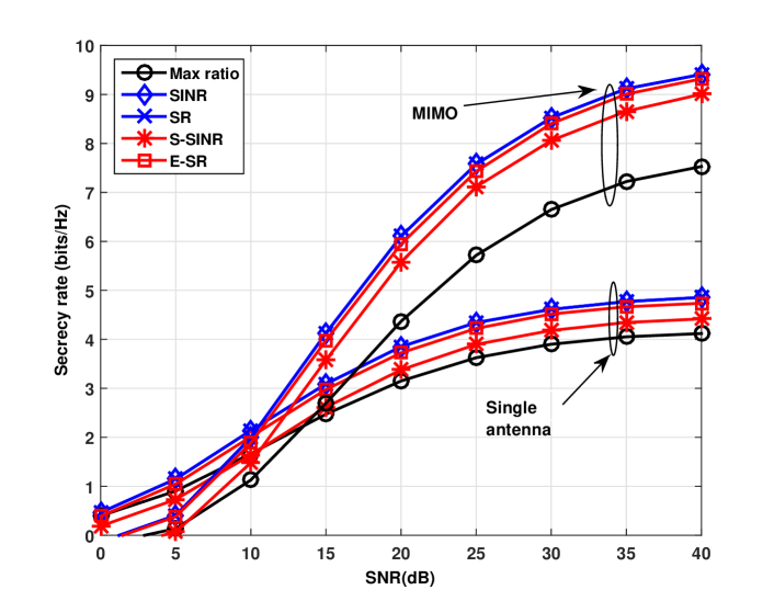
Figure 2: Secrecy-rate performance of relay selection criteria in uncorrelated channels.

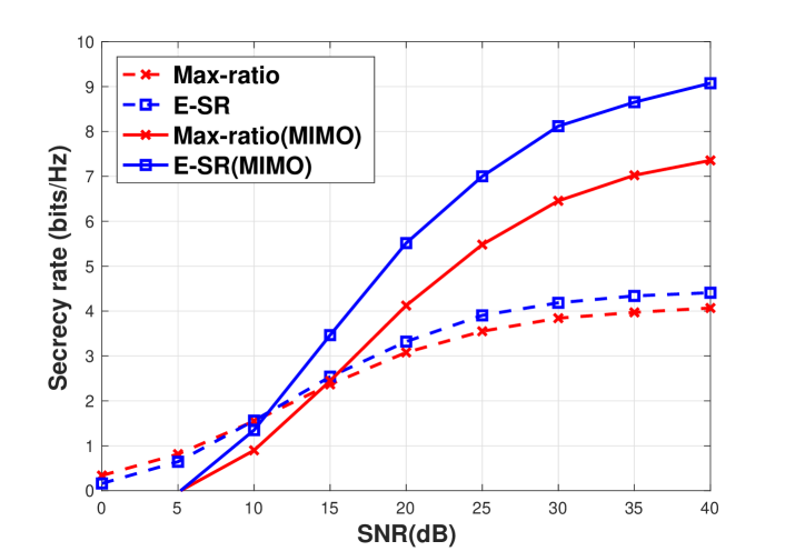
Figure 3: Secrecy-rate performance of relay selection criteria in correlated channels.

In Figs. 2 and 3 we compare the secrecy rate performance in uncorrelated and correlated channels. The results indicate that the proposed E-SR relay selection criterion can improve the secrecy rate in both scenarios. Among the investigated relay selection criteria, E-SR is close to the SR-based scheme that employs CSI to the eavesdroppers and outperforms SINR-based techniques, which are often adopted in the literature [13, 17] and require the CSI of the eavesdroppers.

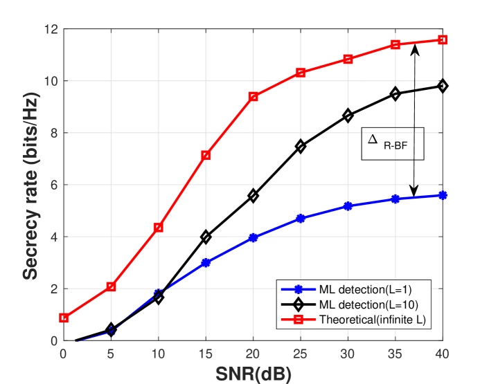
Figure 4: Secrecy-rate performance versus buffer size in uncorrelated channels.

In Fig. 4, the secrecy rate performance with infinite buffer size is compared with buffer size $L=1$ and $L=10$. The theoretical curves are obtained with the expression obtained in Section V for the secrecy rate difference $\Delta_{\rm R-BF}$. According to the results, when the buffer size is increased, the secrecy rate will improve and get close to the theoretical curves.

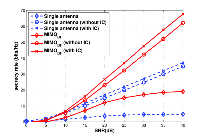
Figure 5: Secrecy rate performance in correlated channels.

In Fig. 5, in a single-antenna scenario, the secrecy-rate performance with the proposed IC scheme and RJFS algorithm is better than that with the conventional algorithm without IC. With IC, the secrecy-rate performance is better than the one without IC, as expected. Compared with the single-antenna scenario, the multiuser MIMO system contributes to the improvement in the secrecy rate as verified in Fig. 5.

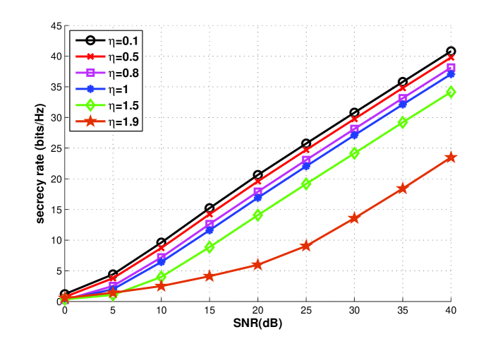
Figure 6: Secrecy rate performance with power allocation and IC.

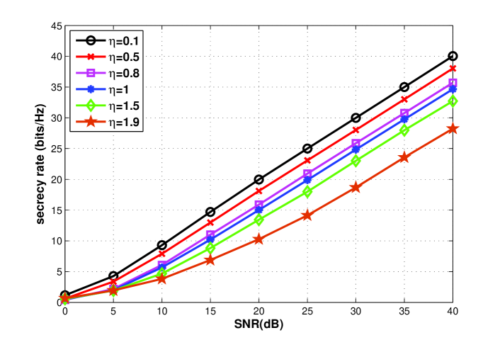
Figure 7: Secrecy rate performance with power allocation and without IC.

In Fig. 6 and Fig. 7, a power allocation technique is considered and the parameter $\eta$ indicates the power allocated to the transmitter. If we assume in the equal power scenario that the power allocated to the transmitter as well as the relays are both $P$, then the power allocated to the transmitter is $\eta P$ and the power allocated to the relays is $(2-\eta)P$. In Fig. 6 and Fig. 7 we can notice that with more power allocated to the transmitter the secrecy rate performance will become worse. Comparing Fig. 6 and Fig. 7, when $\eta<1.5$ the secrecy rate performance in the scenario with IC is better than that without IC. When $\eta>1.5$ the secrecy rate of the system without IC is better than that of the system with IC.

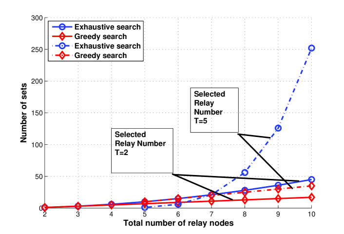
Figure 8: Number of visited sets for the exhaustive and greedy searches.

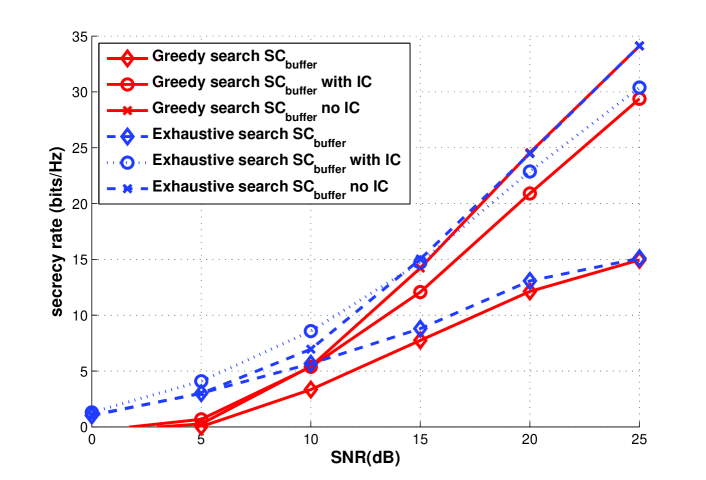
Figure 9: Secrecy rate performance with an exhaustive search and the proposed greedy algorithms.

In Fig. 8 with a fixed number of relays, the computational complexity of the exhaustive and the greedy searches with the RJFS and BF-RJFS algorithms is examined. The results show that the greedy algorithms are substantially simpler than those with the exhaustive search and are suitable for scenarios with a higher number of relays. In Fig. 9 a comparison between the exhaustive search and the greedy algorithms is carried out. The results show that the greedy algorithms approach the same secrecy rate with a much lower complexity than that of the exhaustive search-based techniques.

VII Conclusion

In this work, we have proposed the E-SR approach that allows the maximization of the secrecy rate in buffer-aided relay systems without the need for the CSI of the eavesdroppers. We have also presented algorithms to select a set of relay nodes to enhance the legitimate users’ transmission and another set of relay nodes to perform jamming of the eavesdroppers. The proposed RJFS and BF-RJFS selection algorithms can exploit the use of the buffers in the relay nodes and result in substantial gains in secrecy rate over existing techniques.

[Proof of the proposed E-SR criterion] In this appendix, we include the detailed steps of the derivation of the E-SR criterion.

Proof.

From the original expressions for the achievable rate for users and eavesdroppers, which are shown in (25) and (27), we consider relay selection based on the secrecy rate criterion according to:

$${\mathcal{R}}^{\rm SR}=\arg\max_{\boldsymbol{\varphi}\in\boldsymbol{\Psi}}\sum_{\phi_{i}\in\boldsymbol{\varphi}}\left\{\frac{\det(\boldsymbol{I}+{\boldsymbol{\Gamma}_{r}^{(t)}})}{\det(\boldsymbol{I}+{\boldsymbol{\Gamma}_{e}^{(t)}})}\right\},$$ (85)

where ${\boldsymbol{\Gamma}}_{r}^{(t)}=({\boldsymbol{H}}_{i}{\boldsymbol{R}}_{I}{\boldsymbol{H}}_{i}^{H})^{-1}({\boldsymbol{H}}_{i}{\boldsymbol{R}}_{d}{\boldsymbol{H}}_{i}^{H})$ and ${\boldsymbol{\Gamma}}_{e}^{(t)}=({\boldsymbol{H}}_{e}{\boldsymbol{R}}_{I}{\boldsymbol{H}}_{e}^{H})^{-1}({\boldsymbol{H}}_{e}{\boldsymbol{R}}_{r}{\boldsymbol{H}}_{e}^{H})$. Note that (85) requires ${\boldsymbol{H}}_{e}$, i.e., CSI to the eavesdroppers and that channels from all relays are taken into account for selection. In what follows, we show that a designer can employ an equivalent expression to (85) without resorting to the knowledge of CSI to the eavesdroppers. This requires the assumption that several channel matrices are square. However, it can also be used even for scenarios of non-square channel matrices if the matrices are completed with zeros to ensure a square structure.

In (85), our aim is to circumvent the need for CSI to the eavesdroppers from the denominator. To this end, we assume square matrices which allows the linear algebra property $\det(\boldsymbol{A}\boldsymbol{B})=\det(\boldsymbol{A})\det(\boldsymbol{B})$. Following this approach, the denominator of (85) can be expressed as

$${\det[{\boldsymbol{\Lambda}_{1}}^{-1}{\boldsymbol{\Lambda}_{1}}+{\boldsymbol{\Lambda}_{1}}^{-1}(\boldsymbol{H}_{e}\boldsymbol{R}_{d}\boldsymbol{H}_{e}^{H})]},$$ (86)

where ${\boldsymbol{\Lambda}_{1}}=\boldsymbol{H}_{e}\boldsymbol{R}_{I}\boldsymbol{H}_{e}^{H}$.

Since $\boldsymbol{\Lambda}_{1}$ is assumed to be a square matrix, (86) can be decomposed as

$$\det[{\boldsymbol{\Lambda}_{1}}^{-1}]{\det[{\boldsymbol{\Lambda}_{1}}+(\boldsymbol{H}_{e}\boldsymbol{R}_{d}\boldsymbol{H}_{e}^{H})]},$$ (87)

Using the property of the determinant $\det(\boldsymbol{A}^{-1})=\frac{1}{\det(\boldsymbol{A})}$ [94], we have

$$(\det[{\boldsymbol{\Lambda}_{1}}])^{-1}{\det[{\boldsymbol{\Lambda}_{1}}+(\boldsymbol{H}_{e}\boldsymbol{R}_{d}\boldsymbol{H}_{e}^{H})]},$$ (88)

where

$$\begin{split}(\det[{\boldsymbol{\Lambda}_{1}}])^{-1}&=\big{(}\det[\boldsymbol{H}_{e}\boldsymbol{R}_{I}\boldsymbol{H}_{e}^{H}]\big{)}^{-1}\\ &=\big{(}\det[\boldsymbol{H}_{e}(\sum_{j\neq i}\boldsymbol{U}_{j}{\boldsymbol{s}}_{j}^{(t)}{{\boldsymbol{s}}_{j}^{(t)}}^{H}{\boldsymbol{U}_{j}}^{H})\boldsymbol{H}_{e}^{H}]\big{)}^{-1}\\ &=\big{(}\det[\boldsymbol{H}_{e}\underbrace{{\boldsymbol{U}}_{i}{\boldsymbol{U}}_{i}^{-1}}_{\boldsymbol{I}}(\sum_{j\neq i}\boldsymbol{U}_{j}{\boldsymbol{s}}_{j}^{(t)}{{\boldsymbol{s}}_{j}^{(t)}}^{H}{\boldsymbol{U}_{j}}^{H})\underbrace{{\boldsymbol{U}}_{i}^{H^{-1}}{\boldsymbol{U}}_{i}^{H}}_{\boldsymbol{I}}{\boldsymbol{H}}_{e}^{H}]\big{)}^{-1}\\ &=\big{(}\det[\boldsymbol{H}_{e}{\boldsymbol{U}}_{i}]\det\big{[}(\sum_{j\neq i}{\boldsymbol{U}}_{i}^{-1}{\boldsymbol{U}}_{j}{\boldsymbol{s}}_{j}^{(t)}{{\boldsymbol{s}}_{j}^{(t)}}^{H}{\boldsymbol{U}_{j}}^{H}{\boldsymbol{U}}_{i}^{H^{-1}})\big{]}\\ &\det[{\boldsymbol{U}}_{i}^{H}{\boldsymbol{H}}_{e}^{H}]\big{)}^{-1}\end{split}$$ (89)

and

$$\begin{split}\det[\underbrace{{\boldsymbol{\Lambda}_{1}}+(\boldsymbol{H}_{e}\boldsymbol{R}_{d}{\boldsymbol{H}}_{e}^{H})}_{\boldsymbol{H}_{e}({\boldsymbol{R}}_{I}+{\boldsymbol{R}}_{d}){\boldsymbol{H}}_{e}^{H}}]&=\det[{\boldsymbol{H}}_{e}{\boldsymbol{U}}_{i}]\times\\ &\det\big{[}(\sum_{j\neq i}{\boldsymbol{U}}_{i}^{-1}{\boldsymbol{U}}_{j}{\boldsymbol{s}}_{j}^{(t)}{{\boldsymbol{s}}_{j}^{(t)}}^{H}{\boldsymbol{U}_{j}}^{H}{\boldsymbol{U}}_{i}^{H^{-1}})\\ &+{\boldsymbol{s}}_{i}^{(t)}{{\boldsymbol{s}}_{i}^{(t)}}^{H}\big{]}\det[{\boldsymbol{U}}_{i}^{H}{\boldsymbol{H}}_{e}^{H}]\end{split}$$ (90)

The denominator of the argument in (85) can then be expressed as

$$\begin{split}&(\det[{\boldsymbol{\Lambda}_{1}}])^{-1}{\det[{\boldsymbol{\Lambda}_{1}}+(\boldsymbol{H}_{e}\boldsymbol{R}_{d}\boldsymbol{H}_{e}^{H})]}=\\ &\big{(}\det[\boldsymbol{H}_{e}{\boldsymbol{U}}_{i}]\det\big{[}(\sum_{j\neq i}{\boldsymbol{U}}_{i}^{-1}{\boldsymbol{U}}_{j}{\boldsymbol{s}}_{j}^{(t)}{{\boldsymbol{s}}_{j}^{(t)}}^{H}{\boldsymbol{U}_{j}}^{H}{\boldsymbol{U}}_{i}^{H^{-1}})\big{]}\det[{\boldsymbol{U}}_{i}^{H}{\boldsymbol{H}}_{e}^{H}]\big{)}^{-1}\\ &\quad\det[{\boldsymbol{H}}_{e}{\boldsymbol{U}}_{i}]\det\big{[}(\sum_{j\neq i}{\boldsymbol{U}}_{i}^{-1}{\boldsymbol{U}}_{j}{\boldsymbol{s}}_{j}^{(t)}{{\boldsymbol{s}}_{j}^{(t)}}^{H}{\boldsymbol{U}_{j}}^{H}{\boldsymbol{U}}_{i}^{H^{-1}})+{\boldsymbol{s}}_{i}^{(t)}{{\boldsymbol{s}}_{i}^{(t)}}^{H}\big{]}\\ &\det[{\boldsymbol{U}}_{i}^{H}{\boldsymbol{H}}_{e}^{H}],\end{split}$$ (91)

Using the matrix inverse property $\big{(}\det[{\boldsymbol{A}}]\det[{\boldsymbol{B}}]\det[{\boldsymbol{C}}]\big{)}^{-1}=(\det[{\boldsymbol{C}}^{H}])^{-1}(\det[{\boldsymbol{B}}])^{-1}(\det[{\boldsymbol{A}}^{H}])^{-1}$ [94], we can write

$$\begin{split}&(\det[{\boldsymbol{\Lambda}_{1}}])^{-1}{\det[{\boldsymbol{\Lambda}_{1}}+(\boldsymbol{H}_{e}\boldsymbol{R}_{d}\boldsymbol{H}_{e}^{H})]}=\big{(}\det[{\boldsymbol{H}}_{e}{\boldsymbol{U}}_{i}]\big{)}^{-1}\\ &\big{(}\det\big{[}(\sum_{j\neq i}{\boldsymbol{U}}_{i}^{-1}{\boldsymbol{U}}_{j}{\boldsymbol{s}}_{j}^{(t)}{{\boldsymbol{s}}_{j}^{(t)}}^{H}{\boldsymbol{U}_{j}}^{H}{\boldsymbol{U}}_{i}^{H^{-1}})\big{]}\big{)}^{-1}\\ &\big{(}\det[{\boldsymbol{U}}_{i}^{H}\boldsymbol{H}_{e}^{H}]\big{)}^{-1}\det[{\boldsymbol{H}}_{e}{\boldsymbol{U}}_{i}]\det\big{[}(\sum_{j\neq i}{\boldsymbol{U}}_{i}^{-1}{\boldsymbol{U}}_{j}{\boldsymbol{s}}_{j}^{(t)}{{\boldsymbol{s}}_{j}^{(t)}}^{H}{\boldsymbol{U}_{j}}^{H}{\boldsymbol{U}}_{i}^{H^{-1}})\\ &\quad+{\boldsymbol{s}}_{i}^{(t)}{{\boldsymbol{s}}_{i}^{(t)}}^{H}\big{]}\det[{\boldsymbol{U}}_{i}^{H}{\boldsymbol{H}}_{e}^{H}],\end{split}$$ (92)

By observing the terms above, we notice that that the $1$st term can be canceled by the $4$th term, and that the $3$rd term can be canceled by the $6$th term, resulting in

$$\begin{split}&(\det[{\boldsymbol{\Lambda}_{1}}])^{-1}{\det[{\boldsymbol{\Lambda}_{1}}+(\boldsymbol{H}_{e}\boldsymbol{R}_{d}\boldsymbol{H}_{e}^{H})]}=\\ &\big{(}\det\big{[}(\sum_{j\neq i}{\boldsymbol{U}}_{i}^{-1}{\boldsymbol{U}}_{j}{\boldsymbol{s}}_{j}^{(t)}{{\boldsymbol{s}}_{j}^{(t)}}^{H}{\boldsymbol{U}_{j}}^{H}{\boldsymbol{U}}_{i}^{H^{-1}})\big{]}\big{)}^{-1}\\ &\quad\det\big{[}(\sum_{j\neq i}{\boldsymbol{U}}_{i}^{-1}{\boldsymbol{U}}_{j}{\boldsymbol{s}}_{j}^{(t)}{{\boldsymbol{s}}_{j}^{(t)}}^{H}{\boldsymbol{U}_{j}}^{H}{\boldsymbol{U}}_{i}^{H^{-1}})+{\boldsymbol{s}}_{i}^{(t)}{{\boldsymbol{s}}_{i}^{(t)}}^{H}\big{]}\\ &=\det[{\boldsymbol{I}}+{\boldsymbol{U}}_{i}^{H}{\boldsymbol{R}}_{I}^{-1}{\boldsymbol{U}}_{i}{\boldsymbol{R}}_{d}],\end{split}$$ (93)

By substituting the result in (93) in (85), we obtain the proposed E-SR selection criterion given by

$$\begin{split}{\mathcal{R}}^{\rm S-SR}&=\arg\max_{\boldsymbol{\varphi}\in\boldsymbol{\Psi}}\sum_{\phi_{i}\in\boldsymbol{\varphi}}\left\{\log\Big{(}\frac{\det[\boldsymbol{I}+{\boldsymbol{\Gamma}_{r}^{(t)}}]}{\det(\boldsymbol{I}+{\boldsymbol{\Gamma}_{e}^{(t)}}]}\Big{)}\right\}\\ &=\arg\max_{\boldsymbol{\varphi}\in\boldsymbol{\Psi}}\sum_{\phi_{i}\in\boldsymbol{\varphi}}\left\{\log\Big{(}\frac{\det[\boldsymbol{I}+(\boldsymbol{H}_{i}\boldsymbol{R}_{I}\boldsymbol{H}_{i}^{H})^{-1}(\boldsymbol{H}_{i}\boldsymbol{R}_{d}\boldsymbol{H}_{i}^{H})]}{\det[{\boldsymbol{I}}+({\boldsymbol{H}}_{e}{\boldsymbol{R}}_{I}{\boldsymbol{H}}_{e}^{H})^{-1}({\boldsymbol{H}}_{e}{\boldsymbol{R}}_{r}{\boldsymbol{H}}_{e}^{H})]}\Big{)}\right\}\\ &=\rm{arg}\max_{\boldsymbol{\varphi}\in\boldsymbol{\Psi}}\sum_{\phi_{i}\in\boldsymbol{\varphi}}\left\{\log\Big{(}\frac{\det[\boldsymbol{I}+(\boldsymbol{H}_{i}\boldsymbol{R}_{I}\boldsymbol{H}_{i}^{H})^{-1}(\boldsymbol{H}_{i}\boldsymbol{R}_{d}\boldsymbol{H}_{i}^{H})]}{\det[\boldsymbol{I}+\boldsymbol{U}_{i}^{H}\boldsymbol{R}_{I}^{-1}\boldsymbol{U}_{i}\boldsymbol{R}_{d}]}\Big{)}\right\}\\ &=\arg\max_{\boldsymbol{\varphi}\in\boldsymbol{\Psi}}\sum_{i\in\boldsymbol{\varphi}}\bigg{\{}\log\big{(}\det{\left[\boldsymbol{I}+(\boldsymbol{H}_{i}\boldsymbol{R}_{I}\boldsymbol{H}_{i}^{H})^{-1}(\boldsymbol{H}_{i}\boldsymbol{R}_{d}\boldsymbol{H}_{i}^{H})\right]}\big{)}\\ &\qquad\log\big{(}\det{\left[\boldsymbol{I}+\boldsymbol{U}_{i}^{H}\boldsymbol{R}_{I}^{-1}\boldsymbol{U}_{i}\boldsymbol{R}_{d}\right]}\big{)}\bigg{\}},\end{split}$$ (94)

where the last expression in (94) no longer requires knowledge of CSI to the eavesdroppers ${\boldsymbol{H}}_{e}$ and is equivalent to (40).

∎

References

• [1] C. Shannon, “Communication theory of secrecy systems,” Bell System Technical Journal, The, vol. 28, no. 4, pp. 656–715, Oct 1949.
• [2] A. D. Wyner, “The Wire-Tap Channel,” Bell System Technical Journal, vol. 54, no. 8, pp. 1355–1387, 1975.
• [3] I. Csiszar and J. Korner, “Broadcast channels with confidential messages,” IEEE Transactions on Information Theory, vol. 24, no. 3, pp. 339–348, May 1978.
• [4] F. Oggier and B. Hassibi, “The Secrecy Capacity of the MIMO Wiretap Channel,” IEEE Transactions on Information Theory, vol. 57, no. 8, pp. 4961–4972, Aug 2011.
• [5] T. Liu and S. Shamai, “A Note on the Secrecy Capacity of the Multiple-Antenna Wiretap Channel,” IEEE Transactions on Information Theory, vol. 55, no. 6, pp. 2547–2553, June 2009.
• [6] S. Goel and R. Negi, “Guaranteeing Secrecy using Artificial Noise,” IEEE Transactions on Wireless Communications, vol. 7, no. 6, pp. 2180–2189, June 2008.
• [7] J. Zhang and M. Gursoy, “Collaborative Relay Beamforming for Secrecy,” in 2010 IEEE International Conference on Communications (ICC), May 2010, pp. 1–5.
• [8] Y. Oohama, “Capacity Theorems for Relay Channels with Confidential Messages,” in IEEE International Symposium on Information Theory (ISIT) 2007., June 2007, pp. 926–930.
• [9] H. Wang, K. Huang, Q. Yang, and Z. Han, “Joint source-relay secure precoding for mimo relay networks with direct links,” IEEE Transactions on Communications, vol. 65, no. 7, pp. 2781–2793, July 2017.
• [10] A. Mukherjee, S. Fakoorian, J. Huang, and A. Swindlehurst, “Principles of Physical Layer Security in Multiuser Wireless Networks: A Survey,” IEEE Communications Surveys Tutorials, vol. 16, no. 3, pp. 1550–1573, Third 2014.
• [11] N. Zhao, W. Wang, J. Wang, Y. Chen, Y. Lin, Z. Ding, and N. C. Beaulieu, “Joint beamforming and jamming optimization for secure transmission in miso-noma networks,” IEEE Transactions on Communications, pp. 1–1, 2019.
• [12] B. Li, Y. Zou, J. Zhou, F. Wang, W. Cao, and Y. Yao, “Secrecy outage probability analysis of friendly jammer selection aided multiuser scheduling for wireless networks,” IEEE Transactions on Communications, pp. 1–1, 2019.
• [13] L. Dong, Z. Han, A. P. Petropulu, and H. V. Poor, “Improving Wireless Physical Layer Security via Cooperating Relays,” IEEE Transactions on Signal Processing, vol. 58, no. 3, pp. 1875–1888, March 2010.
• [14] N. Zlatanov and R. Schober, “Buffer-Aided Relaying With Adaptive Link Selection-Fixed and Mixed Rate Transmission,” IEEE Transactions on Information Theory, vol. 59, no. 5, pp. 2816–2840, May 2013.
• [15] G. Chen, Z. Tian, Y. Gong, Z. Chen, and J. Chambers, “Max-Ratio Relay Selection in Secure Buffer-Aided Cooperative Wireless Networks,” IEEE Transactions on Information Forensics and Security, vol. 9, no. 4, pp. 719–729, April 2014.
• [16] J. Huang and A. Swindlehurst, “Wireless Physical Layer Security Enhancement with Buffer-aided Relaying,” in Asilomar Conference on Signals, Systems and Computers, 2013, Nov 2013, pp. 1560–1564.
• [17] A. E. Shafie, D. Niyato, and N. Al-Dhahir, “Enhancing the PHY-Layer Security of MIMO Buffer-Aided Relay Networks,” IEEE Wireless Communications Letters, vol. 5, no. 4, pp. 400–403, Aug 2016.
• [18] A. E. Shafie, A. Sultan, and N. Al-Dhahir, “Physical-Layer Security of a Buffer-Aided Full-Duplex Relaying System,” IEEE Communications Letters, vol. 20, no. 9, pp. 1856–1859, Sept 2016.
• [19] N. Nomikos, T. Charalambous, I. Krikidis, D. N. Skoutas, D. Vouyioukas, and M. Johansson, “A Buffer-Aided Successive Opportunistic Relay Selection Scheme With Power Adaptation and Inter-Relay Interference Cancellation for Cooperative Diversity Systems,” IEEE Transactions on Communications, vol. 63, no. 5, pp. 1623–1634, May 2015.
• [20] N. Nomikos, P. Makris, D. Vouyioukas, D. Skoutas, and C. Skianis, “Distributed joint relay-pair selection for buffer-aided successive opportunistic relaying,” in IEEE 18th International Workshop on Computer Aided Modeling and Design of Communication Links and Networks (CAMAD), 2013, Sept 2013, pp. 185–189.
• [21] J. H. Lee and W. Choi, “Multiuser Diversity for Secrecy Communications Using Opportunistic Jammer Selection: Secure DoF and Jammer Scaling Law,” IEEE Transactions on Signal Processing, vol. 62, no. 4, pp. 828–839, Feb 2014.
• [22] J. Chen, R. Zhang, L. Song, Z. Han, and B. Jiao, “Joint Relay and Jammer Selection for Secure Two-Way Relay Networks,” IEEE Transactions on Information Forensics and Security, vol. 7, no. 1, pp. 310–320, Feb 2012.
• [23] X. Lu and R. C. de Lamare, “Opportunistic relay and jammer cooperation techniques for physical-layer security in buffer-aided relay networks,” in 2015 International Symposium on Wireless Communication Systems (ISWCS), 2015, pp. 691–695.
• [24] X. Lu and R. C. de Lamare, “Relay selection based on the secrecy rate criterion for physical-layer security in buffer-aided relay networks,” in WSA 2016; 20th International ITG Workshop on Smart Antennas, March 2016, pp. 1–5.
• [25] C. Windpassinger, R. F. H. Fischer, T. Vencel, and J. B. Huber, “Precoding in multiantenna and multiuser communications,” IEEE Transactions on Wireless Communications, vol. 3, no. 4, pp. 1305–1316, July 2004.
• [26] T. Wang, R. C. de Lamare, and P. D. Mitchell, “Low-complexity set-membership channel estimation for cooperative wireless sensor networks,” IEEE Transactions on Vehicular Technology, vol. 60, no. 6, pp. 2594–2607, July 2011.
• [27] R. C. D. Lamare, “Joint iterative power allocation and linear interference suppression algorithms for cooperative ds-cdma networks,” IET Communications, vol. 6, no. 13, pp. 1930–1942, Sep. 2012.
• [28] T. Peng, R. C. de Lamare, and A. Schmeink, “Adaptive distributed space-time coding based on adjustable code matrices for cooperative mimo relaying systems,” IEEE Transactions on Communications, vol. 61, no. 7, pp. 2692–2703, July 2013.
• [29] T. Peng and R. C. de Lamare, “Adaptive buffer-aided distributed space-time coding for cooperative wireless networks,” IEEE Transactions on Communications, vol. 64, no. 5, pp. 1888–1900, May 2016.
• [30] J. Gu, R. C. de Lamare, and M. Huemer, “Buffer-aided physical-layer network coding with optimal linear code designs for cooperative networks,” IEEE Transactions on Communications, vol. 66, no. 6, pp. 2560–2575, June 2018.
• [31] R. C. de Lamare and R. Sampaio-Neto, “Reduced-rank adaptive filtering based on joint iterative optimization of adaptive filters,” IEEE Signal Processing Letters, vol. 14, no. 12, pp. 980–983, Dec 2007.
• [32] ——, “Adaptive reduced-rank processing based on joint and iterative interpolation, decimation, and filtering,” IEEE Transactions on Signal Processing, vol. 57, no. 7, pp. 2503–2514, July 2009.
• [33] R. C. de Lamare and R. Sampaio-Neto, “Reduced-rank space-time adaptive interference suppression with joint iterative least squares algorithms for spread-spectrum systems,” IEEE Transactions on Vehicular Technology, vol. 59, no. 3, pp. 1217–1228, March 2010.
• [34] R. C. de Lamare and R. Sampaio-Neto, “Adaptive reduced-rank equalization algorithms based on alternating optimization design techniques for mimo systems,” IEEE Transactions on Vehicular Technology, vol. 60, no. 6, pp. 2482–2494, July 2011.
• [35] S. Xu, R. C. de Lamare, and H. V. Poor, “Distributed compressed estimation based on compressive sensing,” IEEE Signal Processing Letters, vol. 22, no. 9, pp. 1311–1315, Sep. 2015.
• [36] F. L. Duarte and R. C. de Lamare, “Switched max-link relay selection based on maximum minimum distance for cooperative mimo systems,” IEEE Transactions on Vehicular Technology, vol. 69, no. 2, pp. 1928–1941, 2020.
• [37] ——, “Cloud-driven multi-way multiple-antenna relay systems: Joint detection, best-user-link selection and analysis,” IEEE Transactions on Communications, vol. 68, no. 6, pp. 3342–3354, 2020.
• [38] F. L. Duarte and R. C. De Lamare, “C-ran-type cluster-head-driven uav relaying with recursive maximum minimum distance,” IEEE Communications Letters, vol. 24, no. 11, pp. 2623–2627, 2020.
• [39] X. Lu, K. Zu, and R. C.de Lamare, “Lattice-reduction aided Successive Optimization Tomlinson-Harashima Precoding strategies for physical-layer security in wireless networks,” in Sensor Signal Processing for Defence (SSPD), 2014, Sept 2014, pp. 1–5.
• [40] X. Lu, R. C. de Lamare, and K. Zu, “Successive optimization tomlinson-harashima precoding strategies for physical-layer security in wireless networks,” Eurasip Journal on Wireless Communications and Networking, no. 259, 2016.
• [41] K. Zu, R. C. de Lamare, and M. M. Haardt, “Generalized Design of Low-Complexity Block Diagonalization Type Precoding Algorithms for Multiuser MIMO Systems,” IEEE Transactions on Communications, vol. 61, no. 10, pp. 4232–4242, October 2013.
• [42] K. Zu, R. C. de Lamare, and M. Haardt, “Multi-Branch Tomlinson-Harashima Precoding Design for MU-MIMO Systems: Theory and Algorithms,” IEEE Transactions on Communications, vol. 62, no. 3, pp. 939–951, March 2014.
• [43] W. Zhang, R. C. de Lamare, C. Pan, M. Chen, J. Dai, B. Wu, and X. Bao, “Widely linear precoding for large-scale mimo with iqi: Algorithms and performance analysis,” IEEE Transactions on Wireless Communications, vol. 16, no. 5, pp. 3298–3312, 2017.
• [44] R. C. de Lamare, “Massive mimo systems: Signal processing challenges and future trends,” URSI Radio Science Bulletin, vol. 2013, no. 347, pp. 8–20, Dec 2013.
• [45] W. Zhang, H. Ren, C. Pan, M. Chen, R. C. de Lamare, B. Du, and J. Dai, “Large-scale antenna systems with ul/dl hardware mismatch: Achievable rates analysis and calibration,” IEEE Transactions on Communications, vol. 63, no. 4, pp. 1216–1229, April 2015.
• [46] R. C. D. Lamare and R. Sampaio-Neto, “Minimum mean-squared error iterative successive parallel arbitrated decision feedback detectors for ds-cdma systems,” IEEE Transactions on Communications, vol. 56, no. 5, pp. 778–789, May 2008.
• [47] P. Li, R. C. de Lamare, and R. Fa, “Multiple feedback successive interference cancellation detection for multiuser mimo systems,” IEEE Transactions on Wireless Communications, vol. 10, no. 8, pp. 2434–2439, August 2011.
• [48] R. C. de Lamare, “Adaptive and iterative multi-branch mmse decision feedback detection algorithms for multi-antenna systems,” IEEE Transactions on Wireless Communications, vol. 12, no. 10, pp. 5294–5308, October 2013.
• [49] P. Li and R. C. de Lamare, “Distributed iterative detection with reduced message passing for networked mimo cellular systems,” IEEE Transactions on Vehicular Technology, vol. 63, no. 6, pp. 2947–2954, July 2014.
• [50] Y. Cai, R. C. de Lamare, B. Champagne, B. Qin, and M. Zhao, “Adaptive reduced-rank receive processing based on minimum symbol-error-rate criterion for large-scale multiple-antenna systems,” IEEE Transactions on Communications, vol. 63, no. 11, pp. 4185–4201, Nov 2015.
• [51] A. G. D. Uchoa, C. T. Healy, and R. C. de Lamare, “Iterative detection and decoding algorithms for mimo systems in block-fading channels using ldpc codes,” IEEE Transactions on Vehicular Technology, vol. 65, no. 4, pp. 2735–2741, April 2016.
• [52] Z. Shao, R. C. de Lamare, and L. T. N. Landau, “Iterative detection and decoding for large-scale multiple-antenna systems with 1-bit adcs,” IEEE Wireless Communications Letters, vol. 7, no. 3, pp. 476–479, June 2018.
• [53] R. B. Di Renna and R. C. de Lamare, “Adaptive activity-aware iterative detection for massive machine-type communications,” IEEE Wireless Communications Letters, pp. 1–1, 2019.
• [54] ——, “Iterative list detection and decoding for massive machine-type communications,” IEEE Transactions on Communications, vol. 68, no. 10, pp. 6276–6288, 2020.
• [55] M. Yukawa, R. C. de Lamare, and R. Sampaio-Neto, “Efficient acoustic echo cancellation with reduced-rank adaptive filtering based on selective decimation and adaptive interpolation,” IEEE Transactions on Audio, Speech, and Language Processing, vol. 16, no. 4, pp. 696–710, May 2008.
• [56] R. Fa, R. C. de Lamare, and L. Wang, “Reduced-rank stap schemes for airborne radar based on switched joint interpolation, decimation and filtering algorithm,” IEEE Transactions on Signal Processing, vol. 58, no. 8, pp. 4182–4194, Aug 2010.
• [57] L. Landau, R. C. de Lamare, and M. Haardt, “Robust adaptive beamforming algorithms using the constrained constant modulus criterion,” IET Signal Processing, vol. 8, no. 5, pp. 447–457, July 2014.
• [58] L. Qiu, Y. Cai, R. C. de Lamare, and M. Zhao, “Reduced-rank doa estimation algorithms based on alternating low-rank decomposition,” IEEE Signal Processing Letters, vol. 23, no. 5, pp. 565–569, May 2016.
• [59] H. Ruan and R. C. de Lamare, “Robust adaptive beamforming based on low-rank and cross-correlation techniques,” IEEE Transactions on Signal Processing, vol. 64, no. 15, pp. 3919–3932, Aug 2016.
• [60] M. Yukawa, R. C. de Lamare, and I. Yamada, “Robust reduced-rank adaptive algorithm based on parallel subgradient projection and krylov subspace,” IEEE Transactions on Signal Processing, vol. 57, no. 12, pp. 4660–4674, Dec 2009.
• [61] Z. Yang, R. C. de Lamare, and X. Li, “Sparsity-aware space-time adaptive processing algorithms with l1-norm regularisation for airborne radar,” IET Signal Processing, vol. 6, no. 5, pp. 413–423, July 2012.
• [62] S. D. Somasundaram, N. H. Parsons, P. Li, and R. C. de Lamare, “Reduced-dimension robust capon beamforming using krylov-subspace techniques,” IEEE Transactions on Aerospace and Electronic Systems, vol. 51, no. 1, pp. 270–289, January 2015.
• [63] L. Wang and R. C. D. Lamare, “Constrained adaptive filtering algorithms based on conjugate gradient techniques for beamforming,” IET Signal Processing, vol. 4, no. 6, pp. 686–697, Dec 2010.
• [64] H. Ruan and R. C. de Lamare, “Robust adaptive beamforming using a low-complexity shrinkage-based mismatch estimation algorithm,” IEEE Signal Processing Letters, vol. 21, no. 1, pp. 60–64, Jan 2014.
• [65] R. Fa and R. C. D. Lamare, “Reduced-rank stap algorithms using joint iterative optimization of filters,” IEEE Transactions on Aerospace and Electronic Systems, vol. 47, no. 3, pp. 1668–1684, July 2011.
• [66] Z. Yang, R. C. de Lamare, and X. Li, “$l_{1}$-regularized stap algorithms with a generalized sidelobe canceler architecture for airborne radar,” IEEE Transactions on Signal Processing, vol. 60, no. 2, pp. 674–686, Feb 2012.
• [67] R. C. de Lamare and P. S. R. Diniz, “Set-membership adaptive algorithms based on time-varying error bounds for cdma interference suppression,” IEEE Transactions on Vehicular Technology, vol. 58, no. 2, pp. 644–654, Feb 2009.
• [68] R. C. de Lamare and R. Sampaio-Neto, “Reduced-rank space-time adaptive interference suppression with joint iterative least squares algorithms for spread-spectrum systems,” IEEE Transactions on Vehicular Technology, vol. 59, no. 3, pp. 1217–1228, March 2010.
• [69] ——, “Adaptive reduced-rank mmse filtering with interpolated fir filters and adaptive interpolators,” IEEE Signal Processing Letters, vol. 12, no. 3, pp. 177–180, March 2005.
• [70] R. C. de Lamare and R. Sampaio-Neto, “Adaptive reduced-rank mmse filtering with interpolated fir filters and adaptive interpolators,” IEEE Signal Processing Letters, vol. 12, no. 3, pp. 177–180, March 2005.
• [71] ——, “Adaptive interference suppression for ds-cdma systems based on interpolated fir filters with adaptive interpolators in multipath channels,” IEEE Transactions on Vehicular Technology, vol. 56, no. 5, pp. 2457–2474, Sep. 2007.
• [72] L. Wang, R. C. de Lamare, and M. Haardt, “Direction finding algorithms based on joint iterative subspace optimization,” IEEE Transactions on Aerospace and Electronic Systems, vol. 50, no. 4, pp. 2541–2553, October 2014.
• [73] L. Wang, R. C. de Lamare, and M. Yukawa, “Adaptive reduced-rank constrained constant modulus algorithms based on joint iterative optimization of filters for beamforming,” IEEE Transactions on Signal Processing, vol. 58, no. 6, pp. 2983–2997, June 2010.
• [74] S. D. Somasundaram, N. H. Parsons, P. Li, and R. C. de Lamare, “Reduced-dimension robust capon beamforming using krylov-subspace techniques,” IEEE Transactions on Aerospace and Electronic Systems, vol. 51, no. 1, pp. 270–289, January 2015.
• [75] F. G. Almeida Neto, R. C. De Lamare, V. H. Nascimento, and Y. V. Zakharov, “Adaptive reweighting homotopy algorithms applied to beamforming,” IEEE Transactions on Aerospace and Electronic Systems, vol. 51, no. 3, pp. 1902–1915, July 2015.
• [76] Y. V. Zakharov, V. H. Nascimento, R. C. De Lamare, and F. G. De Almeida Neto, “Low-complexity dcd-based sparse recovery algorithms,” IEEE Access, vol. 5, pp. 12 737–12 750, 2017.
• [77] R. C. de Lamare, M. Haardt, and R. Sampaio-Neto, “Blind adaptive constrained reduced-rank parameter estimation based on constant modulus design for cdma interference suppression,” IEEE Transactions on Signal Processing, vol. 56, no. 6, pp. 2470–2482, June 2008.
• [78] N. Song, R. C. de Lamare, M. Haardt, and M. Wolf, “Adaptive widely linear reduced-rank interference suppression based on the multistage wiener filter,” IEEE Transactions on Signal Processing, vol. 60, no. 8, pp. 4003–4016, Aug 2012.
• [79] N. Song, W. U. Alokozai, R. C. de Lamare, and M. Haardt, “Adaptive widely linear reduced-rank beamforming based on joint iterative optimization,” IEEE Signal Processing Letters, vol. 21, no. 3, pp. 265–269, March 2014.
• [80] R. C. de Lamare, R. Sampaio-Neto, and M. Haardt, “Blind adaptive constrained constant-modulus reduced-rank interference suppression algorithms based on interpolation and switched decimation,” IEEE Transactions on Signal Processing, vol. 59, no. 2, pp. 681–695, Feb 2011.
• [81] S. Li, R. C. de Lamare, and R. Fa, “Reduced-rank linear interference suppression for ds-uwb systems based on switched approximations of adaptive basis functions,” IEEE Transactions on Vehicular Technology, vol. 60, no. 2, pp. 485–497, Feb 2011.
• [82] T. G. Miller, S. Xu, R. C. de Lamare, and H. V. Poor, “Distributed spectrum estimation based on alternating mixed discrete-continuous adaptation,” IEEE Signal Processing Letters, vol. 23, no. 4, pp. 551–555, April 2016.
• [83] S. F. B. Pinto and R. C. de Lamare, “Multistep knowledge-aided iterative esprit: Design and analysis,” IEEE Transactions on Aerospace and Electronic Systems, vol. 54, no. 5, pp. 2189–2201, Oct 2018.
• [84] R. C. de Lamare and R. Sampaio-Neto, “Sparsity-aware adaptive algorithms based on alternating optimization and shrinkage,” IEEE Signal Processing Letters, vol. 21, no. 2, pp. 225–229, Feb 2014.
• [85] Y. Cai, R. C. d. Lamare, and R. Fa, “Switched interleaving techniques with limited feedback for interference mitigation in ds-cdma systems,” IEEE Transactions on Communications, vol. 59, no. 7, pp. 1946–1956, July 2011.
• [86] K. Zu, R. C. de Lamare, and M. Haardt, “Generalized design of low-complexity block diagonalization type precoding algorithms for multiuser mimo systems,” IEEE Transactions on Communications, vol. 61, no. 10, pp. 4232–4242, October 2013.
• [87] ——, “Multi-branch tomlinson-harashima precoding design for mu-mimo systems: Theory and algorithms,” IEEE Transactions on Communications, vol. 62, no. 3, pp. 939–951, March 2014.
• [88] L. Zhang, Y. Cai, R. C. de Lamare, and M. Zhao, “Robust multibranch tomlinson-harashima precoding design in amplify-and-forward mimo relay systems,” IEEE Transactions on Communications, vol. 62, no. 10, pp. 3476–3490, Oct 2014.
• [89] L. T. N. Landau and R. C. de Lamare, “Branch-and-bound precoding for multiuser mimo systems with 1-bit quantization,” IEEE Wireless Communications Letters, vol. 6, no. 6, pp. 770–773, Dec 2017.
• [90] C. T. Healy and R. C. de Lamare, “Design of ldpc codes based on multipath emd strategies for progressive edge growth,” IEEE Transactions on Communications, vol. 64, no. 8, pp. 3208–3219, Aug 2016.
• [91] H. Ruan and R. C. de Lamare, “Distributed robust beamforming based on low-rank and cross-correlation techniques: Design and analysis,” IEEE Transactions on Signal Processing, vol. 67, no. 24, pp. 6411–6423, 2019.
• [92] P. Clarke and R. C. de Lamare, “Transmit diversity and relay selection algorithms for multirelay cooperative mimo systems,” IEEE Transactions on Vehicular Technology, vol. 61, no. 3, pp. 1084–1098, 2012.
• [93] I. Krikidis, T. Charalambous, and J. Thompson, “Buffer-Aided Relay Selection for Cooperative Diversity Systems without Delay Constraints,” IEEE Transactions on Wireless Communications, vol. 11, no. 5, pp. 1957–1967, May 2012.
• [94] D. Bernstein, Matrix Mathematics: Theory, Facts, and Formulas (Second Edition).   Princeton University Press, 2009.