Domain Concretization from Examples:
Addressing Missing Domain Knowledge via Robust Planning

Abstract

The assumption of complete domain knowledge is not warranted for robot planning and decision-making in the real world. It could be due to design flaws or arise from domain ramifications or qualifications. In such cases, existing planning and learning algorithms could produce highly undesirable behaviors. This problem is more challenging than partial observability in the sense that the agent is unaware of certain knowledge, in contrast to it being partially observable: the difference between known unknowns and unknown unknowns. In this work, we formulate it as the problem of domain concretization, an inverse problem to domain abstraction. Based on an incomplete domain model provided by the designer and teacher traces from human users, our algorithm searches for a candidate model set under a minimalistic model assumption. It then generates a robust plan with the maximum probability of success under the set of candidate models. In addition to a standard search formulation in the model-space, we propose a sample-based search method and also an online version of it to improve search time. We tested our approach on IPC domains and a simulated robotics domain where incompleteness was introduced by removing domain features from the complete model. Results show that our planning algorithm increases the plan success rate without impacting the cost much.

I INTRODUCTION

Most planning agents rely on complete knowledge of the domain, which could be catastrophic when certain knowledge is missing in the domain model. The fact that the agent is unaware of some domain knowledge makes this problem different and more challenging than partial observability where the agent knows what is missing. That is the difference between known unknowns and unknown unknowns. For example, missing certain state features means that the agent would perceive all states as if those features do not exist. In such cases, traditional planning algorithms can create the same plan under very different scenarios. For similar reasons, standard RL [1], IRL [2], [3], and intention recognition algorithms [4], [5] could be easily misled as a result of incomplete domain knowledge.

We refer to the process required to address this problem as domain concretization, which is inverse to domain abstraction. In this paper, we focus on state abstraction and leave action abstraction in future work. Even though state abstractions in planning have significant computational advantages, if not engineered properly, they can lead to unsound and incomplete domain specifications [6, 7]. Incomplete domain specification also arises naturally from domain ramifications [8] and qualifications [9], [10].

Consider a manufacturing domain where a robot is tasked to deliver a model to a human worker, which is produced by a 3D printer. Depending on how long the model has cooled down before the delivery, the robot is expected to either apply a coolant first or deliver it immediately to the human worker. However, if the temperature is an unknown domain feature to the robot, it may result in immediate delivery regardless of the temperature, which could lead to safety risks.

In this paper, we restrict the domain concretization problem to deterministic domains. We formulate this problem using a STRIPS-like language [11] and provide search methods for candidate models. Our search algorithm generates candidate models based on the incomplete model provided by the domain designer and teacher traces from human users. This problem is first formulated as a search problem in the model space. To expedite the search, we then present a sample-based search method by considering only models that are consistent with the traces. Additionally, we present an online version that is more practical and has a computational advantage as it uses only one trace in each iteration and maintains a small set of models for future refinements.

For planning, our algorithm generates a robust plan that achieves the goal under the maximum number of candidate models. This is done by transforming the planning problem into a Conformant Probabilistic Planning problem [12]. We tested our algorithm on various IPC domains and a simulated robotics domain where incompleteness was introduced by removing specific predicates from the complete domain model. Results show that the robust plan generated by our algorithm increases the plan success rate under the complete model without impacting the cost much.

II RELATED WORK

The ongoing research on state abstraction has established its necessity and computational advantages. There exists work where authors developed abstractions that retained properties of the ground domain. The authors in [13] have studied abstractions that produce optimal behaviors similar to those with the ground domain. In [7], the authors have investigated and categorized several abstraction mechanisms that retain the properties of the ground domain like the Markov property. The fact that the agent’s domain model is missing some domain features in our work makes the model an abstraction of the ground model. Domain concretization is the inverse of domain abstraction: instead of searching for an abstraction, here we are trying to recover the ground domain model from the abstract (incomplete) model.

It may be attempting to solve the domain concretization problem using a POMDP formulation [14], or reinforcement learning methods with POMDPs [15], where the state is partially observable and the agent uses observations to update its belief about the state of the world. Note however that a POMDP still requires complete knowledge about the ground state space, which is not available in our problem formulation due to missing domain knowledge. More specifically, this means that, neither the space of belief states nor the observation function is known, unlike that in POMDP. Hence, POMDP solutions cannot be used to solve our problem.

The agent’s model in our problem could be considered an approximate domain model and hence planning in such a case becomes a type of model-lite planning [16]. Many existing approaches have considered planning in such approximate (or incomplete) domain models. Authors in [17], [18] introduce planning systems that can generate plans for an incomplete domain where actions could be missing some preconditions or effects. Our problem can be viewed as a more general problem where the information of possible missing knowledge (e.g., possible preconditions) is missing.

The idea of learning action model using plan traces has been there for quite some time. While some authors have considered refining incomplete domain models [19], [20], others have focused more on learning action models from scratch [21], [22]. Authors in [23] have used transfer learning to learn the action model using a small amount of training data. In [24], authors have gone one step further by developing an algorithm that can learn action models even when the traces are noisy. One common assumption in all these methods is the complete knowledge of the state space, about which, the agent in our problem, does not have.

III DOMAIN CONCRETIZATION

III-A Problem Analysis

Consider the motivating example of the manufacturing domain mentioned in the previous section. The robot is expected to deliver a 3D model to a human, produced by a 3D printer. The human teacher performs some demonstrations to teach the robot how the task is supposed to be done. The human has the complete domain model $M^{*}$ but the robot’s domain model is incomplete $\widetilde{M}$, where the temperature is an unknown feature. In such a case the traces (demonstrations) are generated by the teacher using $M^{*}$ and projected onto $\widetilde{M}$ that is observed by the robot. In the projection, the robot does not (or cannot) observe the missing feature since it is not present in its domain model (i.e., the robot would consider it irrelevant to the task scenario and/or lacks the appropriate sensor for feature extraction). Before further discussion let us first list the assumptions:

1. The human teacher is rational and the traces are optimal in the complete domain model $M^{*}$.

2. The complete domain model $M^{*}$ is deterministic.

3. The robot still knows about all the possible actions.

4. The unknown features are completely missing from the domain model.

5. The unknown features do not appear in the goal, since the goal is often provided by the human user who is also the teacher.

Given the assumptions mentioned above, an observed (projected) trace would still contain all the actions in the teacher’s trace but the state trajectory associated with it will be viewed differently. To make this clearer, let us have a look at an example trace. Consider the following teacher trace/plan that is observed by the robot in our motivating example:

• Plan $z_{1}$: there is a hot 3D model (that is just printed) in the start state. The action sequence is: $\langle$ apply_coolant, deliver $\rangle$.

In the teacher’s perspective, the state sequence for this action sequence is: $\langle$ {hot}, {wet}, {wet, delivered} $\rangle$, assuming that apply_coolant has two effects, one being making the model wet, and the other being removing hot.

The robot observes the action and state sequences above except for the hot feature, which requires the apply_coolant action to be first applied in the complete model. Since the feature is completely missing in the robot’s model, the apply_coolant action would also be missing it (i.e., the robot is unaware that this action would remove hot from the state or, in other words, make the model cooler). Hence, the state sequence that is observed by the robot would be: $\langle$ {}, {wet}, {wet, delivered} $\rangle$. Hence, it would consider that the apply_coolant action is unnecessary, assuming that the action deliver does not require the model to be wet.

Hence, given the observed initial state {}, in the robot’s model $\widetilde{M}$, the optimal plan for this “same” scenario is (note again that the robot does not observe the hot feature in the initial state):

• Plan $z_{0}$: there is a 3D model in the start state. The action sequence is: $\langle$ deliver $\rangle$.

Obviously, there is an inconsistency here: with the assumption that the teacher is rational and cost captured by plan length, the teacher is expected to never choose anything longer than $z_{0}$. The solution to the problem of domain concretization is hence hinged on addressing this type of inconsistency, which we refer to as plan inconsistency. Let us analyze this further to understand how trace inconsistency can help us concretize our domain models and its limitations. Consider a teacher’s plan $z_{1}$ (under the complete model $M^{*}$). Denote the robot’s optimal plan (under the incomplete model $\widetilde{M}$) for the same observed/projected initial ($\widetilde{s_{0}}$) and goal states ($g$) as $z_{0}$. Two possibilities are here:

1. Cost($z_{1}$) $\neq$ Cost($z_{0}$) – Inconsistency: the teacher has chosen a more or less costly plan than the optimal plan in the robot’s model, which should not occur if the robot’s model is complete. In fact, given our assumptions above, the only possibility here is that Cost($z_{1}$) $>$ Cost($z_{0}$). And that is because when a feature is completely missing in the domain model, it will be missing as both preconditions and effects. Hence, the missing features would only make the incomplete model less constrained to satisfy the goal.

2. Cost($z_{1}$) $=$ Cost($z_{0}$) – Here, there are two possibilities:

   1. $z_{1}$ is a valid plan for $(\widetilde{s_{0}},g)$ in $\widetilde{M}$: Undetermined (deemed consistent): $z_{1}$ could be a valid plan in an incomplete model $\widetilde{M}$ or it could be that $\widetilde{M}$ is complete. Since we cannot decide which case is true here, we will have to wait until inconsistencies are detected.

   2. $z_{1}$ is not a valid plan for $(\widetilde{s_{0}},g)$ in $\widetilde{M}$ – Inconsistency: $z_{1}$ is not a valid plan in the robot’s model but a valid plan in the complete model.

In our problem solution, we address only the cases when any plan inconsistencies above are detected. However, even when all the plan inconsistencies are addressed, it does not mean that the complete model is recovered due to the case of 2.(a) above. On the other hand, as more teacher traces are provided, our solution is expected detect more inconsistencies as long as the complete model is not recovered.

III-B Background

Given our focus on deterministic domains, we use a STRIPS-like language to define our problem. Here, a planning problem is defined by a triplet $P$ $=$ $\langle s_{0}$, $g$, $M\rangle$, where $s_{0}$ is the start state, $g$ is the set of goal prepositions that must be T (true) in the goal state and $M$ is the domain model. The domain model $M$ $=$ $\langle O$, $R\rangle$, where $R$ is the set of predicates and $O$ is the set of operators. The set of prepositions $F$ and the set of actions $A$ are generated by instantiating all the predicates in $R$ and all the operators in $O$ respectively. Hence, we can also define $M$ $=$ $\langle A$, $F\rangle$. A state is either the set of prepositions $s$ $\subseteq$ $F$ that are true or $s_{\bot}$ $=$ {$\bot$}. The state $s_{\bot}$ is a dead state and once it is reached, the goal can never be achieved. The actions change the current state by adding or deleting some prepositions. Each action a $\in$ $A$ is specified by a set of preconditions $Pre(a)$, a set of add effects $Add(a)$ and a set of delete effects $Del(a)$, where $Pre(a)$, $Add(a)$ and $Del(a)\subseteq F$. For a model $M$, the resulting state after executing plan $\pi$ in state $s$ is determined by the transition function $\gamma$, which is defined as follows:

$$\gamma(\pi,s)=\begin{cases}s&\text{if }\!\begin{aligned} \pi=\langle\rangle;\\ \end{aligned}\\ \gamma(\langle a\rangle,\gamma(\pi^{\prime},s))&\!\begin{aligned} \pi=\pi^{\prime}\circ\langle a\rangle.\\ \end{aligned}\end{cases}$$ (1)

In our problem, we use the Generous Execution (GE) semantics as defined in [18] where if an action $a$ is not executable, it does not change the world state $s$. Hence, the transition function $\gamma$ for an action sequence with a single action $a$ and state $s$ under GE semantics is defined as follows:

$$\gamma(\langle a\rangle,s)=\begin{cases}(s\setminus Del(a))\cup Add(a)&\text{if }\!\begin{aligned} Pre(a)\subseteq s;\\ \end{aligned}\\ s&\text{otherwise.}\end{cases}$$ (2)

A plan $\pi$ is a valid plan for a problem $P$ $=$ $\langle s_{0}$, $g$, $M\rangle$ iff $\gamma(\pi,s_{0})\supseteq g$. The cost of a plan $\pi$ is the cumulative cost of all the actions in $\pi$. To make our discussion simpler, we assume that all the actions incur one unit cost. In such a case, the cost of a plan will simply be equal to the plan length. One may also note that our method will still work even if the cost for each action is different.

III-C Motivating Example

(:action open_box
:parameters (?b $–$ box)
:precondition (and (handempty))
:effect (and (box_open ?b)))

(:action grasp
:parameters (?i $–$ item)
:precondition (and (on_shelf ?i) (handempty))
:effect (and (holding ?i) (not (on_shelf ?i))
           (not (handempty))))

(:action place
:parameters (?i1 - item ?b $–$ box)
:precondition (and (holding ?i1) (box_open ?b)
           (box_empty ?b))
:effect (and (item_packed ?i1) (handempty)
           (on_top ?i1 ?b) (not (holding ?i1))
           (not (box_empty ?b))))

(:action stack
:parameters (?i1 - item ?i2 - item ?b - box)
:precondition (and (holding ?i1) (box_open ?b)
           (not_fragile ?i2) (on_top ?i2 ?b))
:effect (and (item_packed ?i1) (handempty)
           (on_top ?i1 ?b) (not (on_top ?i2 ?b))
           (not (holding ?i1))))

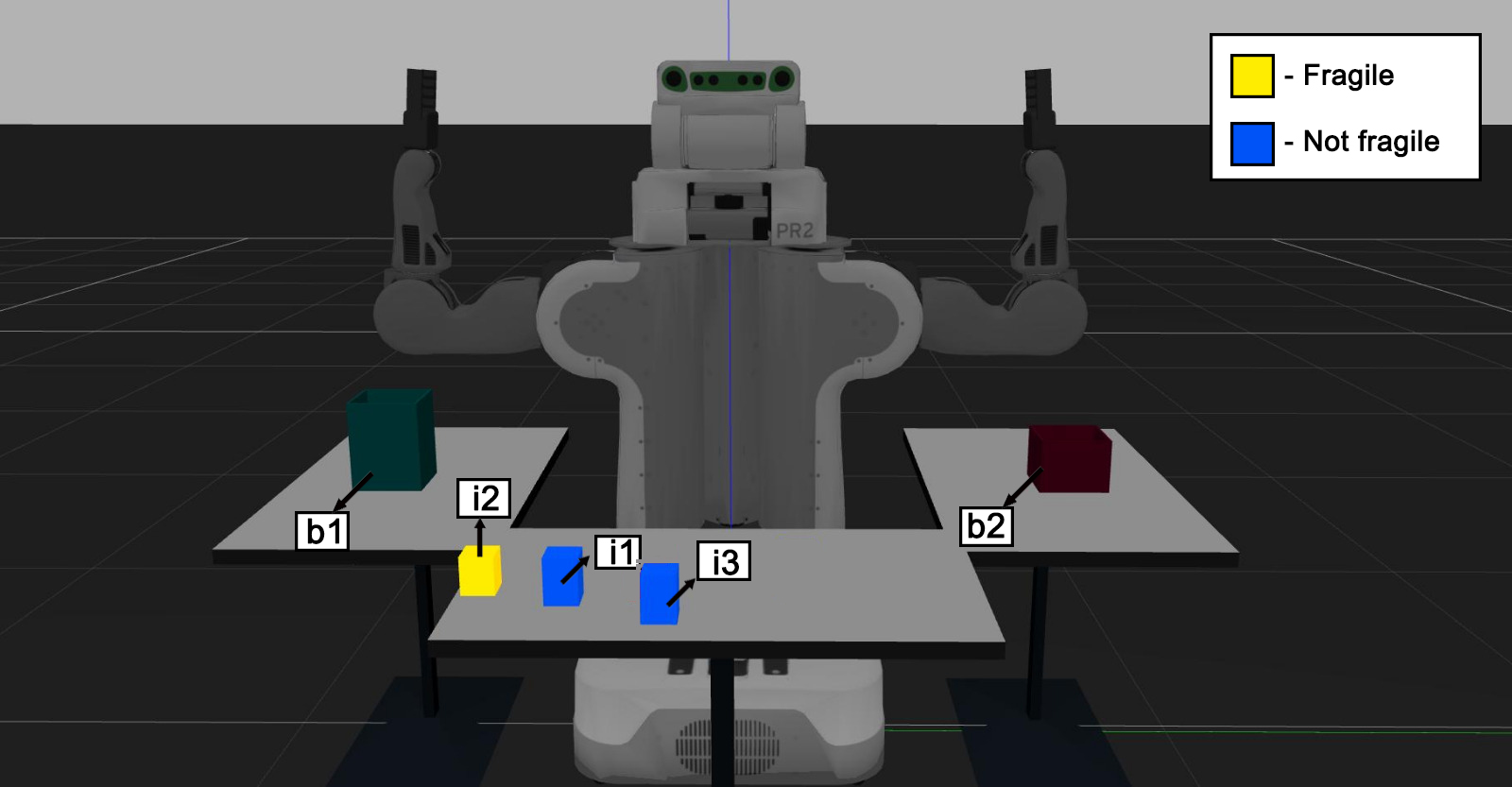
(a)

Figure 1: Packing domain as a runnig example

Complete domain model (denoted by $M^{*}$): The specification of a packing domain is shown in Fig. 1 to motivate our problem. The domain has $4$ operators. As the name suggests, open_box is used to open boxes where items are to be placed. The grasp operator is used to grasp an item. place and stack are used to put items into boxes. place is used when the box is empty and stack is used when the box already contains some items. The goal is to store all items in boxes using the minimum number of boxes. Some of the items may be fragile. For these items, they must not be stacked on. To avoid such situations, a predicate not_fragile is introduced foritems that are not fragile.

Incomplete domain model (denoted by $\widetilde{M}$): In the robot’s domain model that is incomplete, the incompleteness may be due to missing the predicate not_fragile (shown in bold in Fig. 1). In such a case, the robot may choose a plan in which it stacks an item over a fragile item.

III-D Problem Formulation

The incomplete model $\widetilde{M}$ $=$ $\langle\widetilde{O}$, $\widetilde{R}\rangle$ is incomplete in the sense that it is missing some predicates present in the complete domain $M^{*}=\langle O^{*}$, $R^{*}\rangle$. Denote $\widehat{R}$ as the set of missing predicates, such that:

• $\widetilde{R}$ $\subseteq$ $R^{*}$ and $\widetilde{R}=R^{*}\setminus\widehat{R}$

• $\widetilde{Pre(o)}=Pre(o)\setminus\widehat{R}$

• $\widetilde{Add(o)}=Add(o)\setminus\widehat{R}$

• $\widetilde{Del(o)}=Del(o)\setminus\widehat{R}$

Definition 1.

The problem setting of Domain Concretization is defined as a setting where the agent has only access to an incomplete domain model $\widetilde{M}$ and teacher traces under $M^{*}$.

We assume that the human user knows $M^{*}$ so he/she can provide a set of successful teacher traces $\zeta^{*}$ based on $M^{*}$. Each trace $z^{*}$ $\in$ $\zeta^{*}$ is a tuple $\langle s_{0}^{*},g,\tau\rangle$ where $g$ and $s_{0}^{*}$ are the goal and initial state respectively and $\tau$ is an action sequence $\langle a_{1},a_{2},...a_{n}\rangle$ where each $a_{i}$ $\in$ $A^{*}$. Since the robot has incomplete predicate set $\widetilde{R}$, it observes incomplete traces $\widetilde{\zeta}$ = $\langle\widetilde{s_{0}}$, $g$, $\tau\rangle$, where $\widetilde{s_{0}}=s_{0}^{*}\setminus\widehat{R}$. We assume that the robot still has knowledge about all the actions, and hence $\tau$ would not be affected by the incompleteness. Additionally, we also assume that the missing predicate cannot be present in the goal state since the goal is provided by the human user.

Definition 2.

The problem of Planning under Incomplete Domain Knowledge (PIDK) is defined as $\widetilde{P}$ $=$ $\langle\widetilde{s_{0}},g,\widetilde{M},\widetilde{\zeta}\rangle$, which is the problem of generating a plan that has the highest probability of success for $P^{*}$ $=$ $\langle s_{0}^{*},g,M^{*}\rangle$.

III-E Candidate Model Generation

We search for the candidate models that have the minimum number of new predicates and the minimum number of changes introduced into the given incomplete model $\widetilde{M}$. One of the motivations for this assumption could be attributed to the principle of Occam’s Razor [25]. Another reason is due to the fact that here, the model-space search problem has infinite possible solutions as we can always introduce more dummy predicates and still make the model generate the given traces. This is somewhat similar to the unidentifiability problem in reward learning [26], [27], [28] and we call it the problem of model unidentifiability.

We transform the problem of generating candidate models to a search problem in the model space. We define a variable $\sigma$ whose value indicates the number of new predicates that are going to be added. Initially, $\sigma$ is set to 1 and is gradually increased if no models are found for the current value. Further, we define a set $X$ as the set of possible typed predicates (generated from all possible type combinations) for each new predicate. Each state in the search space is a domain model ($M$) generated by adding one or more predicates from $X$ to one or more possible missing positions in the incomplete domain model ($\widetilde{M}$). Since these predicates could also be present in the start state, each candidate model $M$ is verified against one or multiple possible start states $s_{0}$, based on the prepositions added to $\widetilde{s_{0}}$ (details in the search section). The model $M$ is accepted as a candidate model if it passes the model test below for at-least one $s_{0}$. Our model-space search is defined as follows:

• Initial State: $\widetilde{M}$

• Action Set ($\Lambda$): $\alpha^{Pre(o)}_{\chi}$ $($or $\alpha^{Add(o)}_{\chi}/\alpha^{Del(o)}_{\chi})\in\Lambda$,

  $\forall\chi\in X$ and $\forall o\in O$ where $O\in M$.

  The actions in the model-space search represent a predicate $\chi$ being added to the $Pre(o)$ $($or $Add(o)/Del(o))$ of the current model $M$.

• Successor Function ($T$): $T(M,\alpha^{Pre(o)}_{\chi})=M^{\prime}$.

  $T$ produces new model $M^{\prime}$ where $R^{\prime}=R\cup\chi$ and $Pre(o^{\prime})=Pre(o)\cup\chi$ where $o^{\prime}\in O^{\prime}$ and $o\in O$. Similarly, we can define $T(M,\alpha^{Add(o)}_{\chi})$ and $T(M,\alpha^{Del(o)}_{\chi})$.

• Model (Goal) Test: $C_{1}(M)$ $\land$ $C_{2}(M)$ $\land$ $C_{3}(M)$.

  $C_{1}(M)$, $C_{2}(M)$ and $C_{3}(M)$ are defined as follows-

  • Plan Validity Test, $C_{1}(M)$ is True if :

    $$\gamma^{M}(\tau,s_{0})\supseteq g;\forall\langle\widetilde{s_{0}},g,\tau\rangle\in\widetilde{\zeta}$$ (3)

    This ensures that the traces are executable and achieve the goal under $M$. This condition essentially detects the type of inconsistency mentioned in case 2.(b) of the problem analysis section (III.A).

  • Well-Justification Test, $C_{2}(M)$ is True if :

    $$\forall a_{i}\in\tau,\gamma^{M}(\tau\setminus\{a_{i}\},s_{0})\nsupseteq g;\forall\langle\widetilde{s_{0}},g,\tau\rangle\in\widetilde{\zeta}$$ (4)

    This ensures that the traces are well-justified [29] in $M$, which means that if any action is removed from the trace the goal will not be achieved. This condition detects the type of inconsistency mentioned in case 1 of the problem analysis section (III.A).

  • Plan Optimality Test, $C_{3}(M)$ is True if :

    $$Cost(\pi^{M})=Cost(\tau);\forall\langle\widetilde{s_{0}},g,\tau\rangle\in\widetilde{\zeta}$$ (5)

    where $\pi^{M}$ is the optimal plan for problem $P$ $=$ $\langle s_{0}$, $g$, $M\rangle$; $Cost(\pi^{M})$ and $Cost(\tau)$ represents plan cost of $\pi^{M}$ and $\tau$ respectively. This condition ensures that the traces are optimal under $M$. This condition detects the type of inconsistency mentioned in case 1 of the problem analysis section (III.A).

In the packing domain, let $\tau$ = $\langle$open_box b1, grasp i1, place i1 b1, grasp i2, stack i2 i1 b1, open_box b2, grasp i3, place i3 b2$\rangle$. Applying the algorithm to $\tau$ and $\widetilde{M}$, $C_{3}$ will fail because, optimal plan, $\pi^{M}$ = $\langle$open_box b1, grasp i1, place i1 b1, grasp i2, stack i2 i1 b1, grasp i3, stack i3 i2 b1$\rangle$, is less costly than $\tau$. This indicates that the trace is inconsistent as mentioned in the case 1 of the problem analysis (III.A) section.

Theorem 1: $C_{1}(M)$ and $C_{3}(M)$ are necessary and sufficient to ensure that the model $M$ can generate $\tau$, $\forall\langle\widetilde{s_{0}},g,\tau\rangle$ $\in$ $\widetilde{\zeta}$.

Proof: If $C_{1}(M)$ is true then $\gamma^{M}(\tau,s_{0})\supseteq g$ which means $\tau$ is a valid plan for $\langle s_{0}$, $g$, $M\rangle$. Also, if $C_{3}(M)$ is true then cost of optimal plan of $M$ equals cost of $\tau$ which implies $\tau$ has minimum cost under $M$. Hence, by definition $\tau$ is the optimal plan for the given problem under model $M$. Since this is true for all $\tau$, it can be concluded that $M$ can generate $\tau$ $\forall\langle\widetilde{s_{0}}$, $g$, $\tau\rangle$ $\in$ $\widetilde{\zeta}$. Similarly, if a model M can generate $\tau$ for a problem $\langle s_{0}$, $g$, $M\rangle$ then $\tau$ an optimal plan for the problem. Hence, by definition of optimal plan, $\tau$ is valid and has minimum cost which implies that it satisfies $C_{1}(M)$ and $C_{3}(M)$. This proves that the model test is sound and complete.

Theorem 2: $C_{2}(M)$, is a necessary condition for a trace $\tau$ where $\langle\widetilde{s_{0}},g,\tau\rangle$ $\in$ $\widetilde{\zeta}$ to be optimal.

Proof: This could be proven by contradiction. Assume that model $M$ doesn’t satisfy $C_{2}(M)$ but still $\tau$ is an optimal plan for $M$. This implies that for some action $a_{i}$, $\tau\setminus\{a_{i}\}$ is a valid plan. Hence, there is a valid plan $\tau\setminus\{a_{i}\}$ which has lesser cost than $\tau$ as $Cost(\tau\setminus\{a_{i}\})=Cost(\tau)-Cost(a_{i})$. This implies that $\tau$ is not an optimal plan which contradicts the initial assumption. Hence proved.

$C_{3}(M)$ requires the computation of an optimal plan which is costly. Hence, we check for $C_{3}(M)$ only if $C_{2}(M)$ fails to reduce the search time. Theorem 2 ensures that this process will not lose any candidate models.

Search: This formulation can be solved by any standard search algorithm and we chose a uniform cost search. The cost of the path from $M$ to $M^{\prime}$ is the number of changes introduced into the domain model $M$ to generate $M^{\prime}$. The search starts with $\widetilde{M}$ as the initial state for the model-space search. Using the action set $\Lambda$ and the transition function $T$, the set of next models is generated and put into a priority queue. The model with the least cost is then popped and passed through the model test. The model is tested with multiple $s_{0}$ for each trace. If $X^{\prime}$ ($X^{\prime}\subset X$) is the set of predicates added to the current domain model $M$, we generate $U$ as a set of all the prepositions that can be instantiated from each predicate in $X^{\prime}$. Now, $s_{0}=\widetilde{s_{0}}\cup\mu$ where $\mu\in{\mathfrak{P}}(U)$. Each $\mu$ is chosen such that $|\mu|$ is minimum. First we test with $|\mu|$ = 0 and if the model test is passed we do not go further. If it fails, we test with every $\mu$ such that $|\mu|$ = 1. This process goes on until a predefined threshold is reached and in that case model test fails. Setting this threshold to 0 denotes an assumption that missing predicate could never be present in the start state.

Now, If the model test is passed, all the models having the same cost are popped and tested. Each model that passes the model test becomes a candidate model. If the model test fails, the set of next models is generated in a similar way as mentioned before. This process continues until some model passes the model test or the cost increases to be above a predefined threshold. In the latter case, $\sigma$ is increased by $1$ and the whole search starts again. In the end, we obtain sets of models such that, within each set of models, $s_{0}$ used to satisfy the model test remains the same. Each model could be in multiple sets based on the $s_{0}$’s that satisfy the model test. The candidate model set $\mathcal{M}$ is a weighted union of these sets of models based on how many times each model appears in those sets.

In our example packing domain in Fig 1, we start with $\widetilde{M}$ as the model $M$ and $\sigma$ = 1. Denote the missing predicate as pred_1. Since $M$ fails $C_{3}(M)$, the search is started by generating $X$. $X$ includes all the possible typed predicates like (pred_1 ?b - box), (pred_1 ?b - box ?i - item), etc. Using $X$, we generate the set $\Lambda$ that includes all the possibilities where the predicates in $X$ can be added, like $\alpha^{Pre(open\_box)}_{\chi}$ $\forall\chi\in X$, which means $\chi$ will be added to the preconditions of operator open_box. Using the current model $M$, $T$ and $\alpha\in\Lambda$, we generate model $M^{\prime}$.

III-F Generating candidate models using sample-based search

To contain the computational complexity, we further present a sample-based search to reduce the search space. The idea is to return information for refining the model to satisfy the traces only, instead of checking all possibilities. The action set $\Lambda^{\prime}$ now is a set of actions that each encodes multiple simultaneous changes. Such a process should also decide what $s_{0}$ to use for a model $M$ in the model test. This process is similar as before except that if a model fails the model test, instead of returning false, it returns a set of actions, $B\subseteq\Lambda^{\prime}$ that will be used to generate models for the next step. Instead of checking the model $M$ for all possible $s_{0}$’s, we check for the ones that are returned along with the action set. The returned action set $B$ is as follows:

• Unsatisfied Precondition: Here, the trace is not executable in $M$ because of some unsatisfied precondition. This means, $C_{1}(M)$ is false and, for an action $a_{i}\in\tau$, $1\leq i\leq|\tau|$, $Pre(a_{i})\nsubseteq\gamma^{M}(\langle a_{1},a_{2},...a_{i-1}\rangle,s_{0})$. Then, the returned action set $B=\{\{\alpha^{Add(o_{j})}_{\chi}\}\}$, $\forall a_{j}\in\tau$ and $\forall\chi\in X$, where $o_{j}$ is the operator corresponding to action $a_{j}$ and $1\leq j\leq i-1$. Also, possible additions to start state $s_{0}$ will be $Pre(a_{i})\setminus\gamma^{M}(\langle a_{1},a_{2},...a_{i-1}\rangle,s_{0})$. This is because missing preposition could either be present in the add effect of any of the previous actions or in the start state. This addresses the type of trace inconsistency mentioned in case 2.(b) of the problem analysis section (III.A).

• Un-justified action: This happens when some action in the trace is not well-justified in $M$. This means, $C_{2}(M)$ is false and for some action $a_{i}$, $\gamma^{M}(\tau\setminus\{a_{i}\},s_{0})\supseteq g$. Then, the returned action set $B=\{\{\alpha^{Add(o_{i})}_{\chi},\alpha^{Pre(o_{j})}_{\chi}\}\}\cup\{\{\alpha^{Add(o_{i})}_{\chi},\alpha^{Pre(o_{j})}_{\chi},\alpha^{Del(o_{j})}_{\chi}\}\}$ $\forall a_{j}\in\tau$ and $\forall\chi\in X$. $o_{i}$ and $o_{j}$ are operators corresponding to actions $a_{i}$ and $a_{j}$ respectively and $i+1\leq j\leq|\tau|$. Intuitively, this generates $B$ such that $a_{i}$ cannot be removed from $\tau$ which makes it well-justified under $M$. This addresses the type of trace inconsistency mentioned in case 1 of the problem analysis section (III.A).

• Sub-optimal Trace: This happens when the optimal plan under $M$ is shorter than the trace. Here, $C_{3}(M)$ becomes false, which means there has to be some action that was not possible in $\tau$ under $M^{*}$ but was possible in $\pi^{M}$ under $M$. Hence, the operator corresponding to that action is missing some precondition. In such a case, $\exists a_{i},a^{\prime}_{i}$ such that $a_{i}\in\tau$ and $a^{\prime}_{i}\in\pi^{M}$ and $a_{i}\neq a^{\prime}_{i}$, $1\leq i\leq n$ $(n=|\pi^{M}|)$. Then, the returned action set $B=\{\{\alpha^{Pre(o_{j})}_{\chi}\}\}\cup\{\{\alpha^{Pre(o_{j})}_{\chi},\alpha^{Del(o_{j})}_{\chi}\}\}$ $\forall a^{\prime}_{j}\in\pi^{M}$, where $o_{j}$ is the operator corresponding to $a^{\prime}_{j}$ and $i\leq j\leq n$. This addresses the type of trace inconsistency mentioned in case 1 of problem analysis section (III.A).

For the packing domain in Fig. 1, consider $\tau$ = $\langle$open_box b1, grasp i1, place i1 b1$\rangle$. If some model $M$ is missing the predicate (box_open ?b), $C_{2}(M)$ will fail because the goal will be achieved even after the deletion of open_box b1 from $\tau$. In that case, $B=\{\{\alpha^{Add(open\_box)}_{\chi},\alpha^{Pre(grasp)}_{\chi}\}$,$\{\alpha^{Add(open\_box)}_{\chi}$, $\alpha^{Pre(place)}_{\chi}\}\}\cup\{\{\alpha^{Add(open\_box)}_{\chi},\alpha^{Pre(grasp)}_{\chi},\alpha^{Del(grasp)}_{\chi}\}$, $\{\alpha^{Add(open\_box)}_{\chi},\alpha^{Pre(place)}_{\chi},\alpha^{Del(place)}_{\chi}\}\}$ $\forall\chi\in X$.

Theorem 3: (Soundness) The candidate models found by the sample-based search process can generate all the given traces, with the minimum number of changes to the incomplete model $\widetilde{M}$.

Proof: This is pretty straightforward as while generating the action set $B$ in the sample-based search method, the process checks to see if the conditions ($C_{1}(M)$, $C_{2}(M)$ and $C_{3}(M)$) are satisfied. It accepts the model as a candidate model only if these are satisfied. Using Theorem 1, it can be said that if the sample-based search process finds a candidate model, the candidate model will be able to generate all the given traces. Uniform cost search ensures that the changes between the candidate models and the given incomplete domain model $\widetilde{M}$ are minimum. Hence Proved.

Theorem 4: (Completeness) The sample-based search finds all the models satisfying the model test with the minimum number of changes to the incomplete model $\widetilde{M}$.

Proof: We prove this by induction. Let us start from the first iteration through all the traces. In this iteration, since the unknown features are completely missing from the incomplete domain model $\widetilde{M}$, it makes the model a less constrained model than the complete model $M$ for achieving any goal. Hence, a trace will always be achieving the goal in $\widetilde{M}$ when it works under the complete model. This means $C_{1}(M)$ will always be satisfied. For any trace, $C_{2}(M)$ can still be false and in that case, it means that there is some action $a_{i}$ that is not well-justified under $\widetilde{M}$. To make that action well-justified, it is necessary that $a_{i}$ has some add effect that is a precondition for one of the subsequent actions in the trace. All these possibilities are included in the set $B$ discussed above. These changes are necessary to ensure that model $M$ satisfies the conditions.

Similarly, for any trace, $C_{3}(M)$ can also be false and in that case, the model $\widetilde{M}$ must have an optimal plan with shorter (lesser cost) than the trace. In that case, to satisfy $C_{3}(M)$, this optimal plan must be inexecutable in the complete model. This is necessarily achieved by updating $\widetilde{M}$ to add new preconditions to actions following the action $a_{i}$ up to which the trace and this optimal plan are the same. Here also, $B$ contains all the possibilities. Since a delete effect may also appear as a precondition in the same action, each option in $B$ that includes the addition of a new predicate to the preconditions comes with a paired option that includes the addition of the new predicate to the delete effects as well.

Now let us assume that for the first $k$ iterations, all necessary changes to $\widetilde{M}$ with all possibilities are considered. For the $(k+1)^{th}$ iteration, since in the previous iterations we have added some new preconditions, the current (intermediate) model $M$ may no longer be less constrained than the complete model for achieving a goal. Hence, for any trace, it might not be achieving its goal in $M$, which means that $C_{1}(M)$ may fail. In this case, it is necessary that there is some action $a_{i}$ for which one of the preconditions is not satisfied. In this case, to make the trace executable, the only possibilities are to add the predicate (for the unsatisfied precondition) either to the add affects of some action before $a_{i}$ in the trace, or to the start state. Again we can see that $B$ includes all the possibilities in which predicate could be added to make the model satisfy this condition for each trace. For the $(k+1)^{th}$ iteration we can use similar reasoning as in the first iteration to argue that $B$ includes all the possibilities for $C_{2}(M)$ and $C_{3}(M)$ as well.

Hence, by induction, we show that the sample-based search includes all the possible ways in which the given incomplete model can be modified to satisfy all the given traces. The Uniform Cost Search (UCS) ensures that the changes are minimal. Hence, the sample-based search process will find all the candidate models with the minimum number of changes.

III-G Generating candidate models using online search

In the real world, it is desirable to have an online search method that takes traces into account as they arrive. The search procedure is similar to the sample-based method above and starts with the incomplete model $\widetilde{M}$. The difference being that the model test is performed against just one trace at a time. Within each iteration, the search continues till it finds $\mathcal{M}$. Once $\mathcal{M}$ is generated, it begins the next iteration by adding models in $\mathcal{M}$ (from the previous iteration) to the priority queue and then starting the search process again. It continues iterating until all available traces are checked.

In terms of computation, on average, the online sample-based search is expected to perform better. This is because in each iteration it uses only those models that satisfy the traces in the previous iterations. This restricts the number of models to be checked in each iteration since it is only constrained by one trace at any time. It makes the online method highly dependent on the sequence of traces and not guaranteed to find the complete model. This is because it could find some incorrect model $M_{1}$, higher in the search-tree and at the same level reject some model $M_{2}$ that would have lead to the correct model by introducing a few more changes (deeper in the tree). In that iteration, the online search would not consider models that are deeper than $M_{1}$. Since in the next iteration only $M_{1}$ will be considered, there is a possibility that the correct model would never be found.

III-H Planning under Incomplete Domain Knowledge

After generating the set of candidate models $\mathcal{M}$, we find a robust plan for $\widetilde{P}$ $=$ $\langle\widetilde{s_{0}},g,\widetilde{M},\widetilde{\zeta}\rangle$ such that it has the highest probability of achieving the goal under the weighted set of candidate models $\mathcal{M}$. Similar to [18], we compile the problem of generating a robust plan into a Conformant Probabilistic Problem (CPP). A Conformant Probabilistic Problem [12] is defined as $P’=\langle I$, $g$, $D$, $\rho\rangle$ where $I$ is the belief over the initial state, $g$ is set of propositions that needs to be T for goal state, $D$ is the domain model and $\rho$ is the acceptable goal satisfaction probability. The domain model $D=\langle F^{\prime}$, $A’\rangle$, where $F’$ is the set of prepositions and $A’$ is the set of actions. Each $a’\in A’$ has the set of preconditions $Pre(a’)\subseteq F’$ and $E(a’)$, the set of conditional effects. Each $e’\in E(a’)$ is a pair of $con(e’)$ and ȯ$(e’)$ where $con(e’)\subseteq F’$ which enables $e’$ and ȯ$(e’)$ is a set of outcomes $\epsilon$. The outcome $\epsilon$ is a triplet $\langle Pr(\epsilon)$, $add(\epsilon)$, $del(\epsilon)\rangle$ where $add(\epsilon)$ adds prepositions to and $del(\epsilon)$ deletes prepositions from the current model with probability $Pr(\epsilon)$.

A compilation that translates the original planning problem $\widetilde{P}$ to a conformant probabilistic planning problem $P’$ is defined as follows:

• For each candidate model $M_{i}\in\mathcal{M}$ a preposition $m_{i}$ is introduced. Let the set of these prepositions be $\widehat{M}$. Further, a set $\widehat{F}=\bigcup\limits_{i=1}^{n}F_{i}$ is introduced, where $F_{i}$ is the set of prepositions instantiated by predicates $R_{i}\in M_{i}$ where $M_{i}\in\mathcal{M}$ and n is the total number of model in $\mathcal{M}$. For the compiled problem set of prepositions $F^{\prime}=\widehat{M}\cup\widehat{F}$.

• For each model $M_{i}\in\mathcal{M}$, $U^{\prime}_{i}$ is created which is the set of new prepositions that were not present in $\widetilde{M}$. Using this, now a domain model is created $D$ from $\widetilde{M}$ as follows:

  • A new action $a^{\prime}_{0}$ that initializes the start state with new/missing prepositions is introduced. The action $a^{\prime}_{0}$ is defined as $Pre(a^{\prime}_{0})=\emptyset$. $\forall m_{i}\in\widehat{M}$, a conditional effect $e^{\prime}_{i}\in E(a^{\prime}_{0})$ is created such that $con(e^{\prime}_{i})=\{m_{i}\}$ and each outcome $\epsilon_{j}\in$ ȯ$(e^{\prime}_{i})$ has $add(\epsilon_{j})=\mu^{\prime}$ and $del(\epsilon_{j})=\emptyset$ where $\mu^{\prime}\in{\mathfrak{P}}(U^{\prime}_{i})$. For each outcome, $Pr(\epsilon_{j})=1/|{\mathfrak{P}}(U^{\prime}_{i})|$. This essentially initializes the start state for each model $M_{i}$, considering all the possibilities for new prepositions to be present in it with equal probability. In the packing domain, if $U^{\prime}_{i}$ $=$ $\{$ (pred_0 i1), (pred_0 i2)$\}$, all the possibilities are $\{\}$, $\{$(pred_0 i1)$\}$, $\{$(pred_0 i1)$\}$, $\{$(pred_0 i1), (pred_0 i2)$\}$. All of these will be considered to be present in the start state with equal probability for each, which is $0.25$ here.

  • For each action $a\in\widetilde{A}$ in $\widetilde{M}$, if model $M_{i}\in\mathcal{M}$ adds a preposition $u^{\prime}_{i}\in U^{\prime}_{i}$ to $\widetilde{Pre(a)}$, a conditional rule $e_{i}\in E(a)$ is created, such that $con(e_{i})=\widetilde{Pre(a)}\cup\{m_{i}\}\cup\{u^{\prime}_{i}\}$, $add(e_{i})=\widetilde{Add(a)}$ and $del(e_{i})=\widetilde{Del(a)}$, $m_{i}\in\widehat{M}$ is the binary predicate corresponding to $M_{i}$. For example, if in model $M_{i}$, action place i1 has the new preposition (pred_0 i1) in it’s precondition, then the action in the compiled domain will have a conditional rule where $con(e_{i})=\widetilde{Pre({\tt place}\,{\tt i1})}\cup\{m_{i}\}\cup\{$(pred_0 i1)$\}$ and $add(e_{i})$ and $del(e_{i})$ will remain the same.

  • For each action $a\in\widetilde{A}$ in $\widetilde{M}$, if model $M_{i}\in\mathcal{M}$ adds a preposition $u^{\prime}_{i}\in U^{\prime}_{i}$ to $\widetilde{Add(a)}$, a conditional rule $e_{i}\in E(a)$ is created, such that $con(e_{i})=\widetilde{Pre(a)}\cup\{m_{i}\}$, $add(e_{i})=\widetilde{Add(a)}\cup\{u^{\prime}_{i}\}$, $del(e_{i})=\widetilde{Del(a)}$, $m_{i}\in\widehat{M}$, is the binary predicate corresponding to $M_{i}$.

  • For each action $a\in\widetilde{A}$ in $\widetilde{M}$, if model $M_{i}\in\mathcal{M}$ adds a preposition $u^{\prime}_{i}\in U^{\prime}_{i}$ to $\widetilde{Del(a)}$, a conditional rule $e_{i}\in E(a)$ is created, such that $con(e_{i})=\widetilde{Pre(a)}\cup\{m_{i}\}$, $add(e_{i})=\widetilde{Add(a)}$, $del(e_{i})=\widetilde{Del(a)}\cup\{u^{\prime}_{i}\}$, $m_{i}\in\widehat{M}$, is the binary predicate corresponding to $M_{i}$.

  The modified domain becomes $D$ for the problem $P’$.

• The initial belief state $I=(\bigwedge\limits_{f\in\widetilde{s_{0}}}f)\land(oneof(m_{1},m_{2},...m_{n}))$ where $oneof$ returns T when exactly one of its input is T. The probability of each $m_{i}$ is equal to its weight in $\mathcal{M}$ and all the other prepositions are certain.

• In the compiled problem, $\rho^{\prime}$ = $\rho$ represents the probability of success of the conformant plan generated in the problem $\widetilde{P}$.

The process of generating the robust plan is quite straightforward. Initially, $\rho$ = 1, and a conformant plan is calculated for the given problem using conformant probabilistic planner. If a conformant plan is not found $\rho$ is decreased by $\Delta$ until one is found. The plan so obtained is a robust plan for problem $\widetilde{P}$ $=$ $\langle\widetilde{s_{0}},$ $g,$ $\widetilde{M},\widetilde{\zeta}\rangle$ and has the highest probability of success given the weighted set of candidate models $\mathcal{M}$.

Theorem 5: If $\pi^{\prime}=\langle a^{\prime}_{0},a^{\prime}_{1},a^{\prime}_{2},a^{\prime}_{3},...a^{\prime}_{n}\rangle$ is a plan for the complied problem $P^{\prime}$ with goal probability $\rho$ then, $\rho$ is also the probability of success of the plan $\pi=\langle a_{1},a_{2},a_{3},...a_{n}\rangle$ in the problem $\widetilde{P}$.

Proof: The compilation defines a bijective mapping between each state $i_{j}\in I$ of the problem $P^{\prime}$ and each model $M_{j}\in\mathcal{M}$ of the problem $\widetilde{P}$. Also, the probability of $i_{j}$ in $I$ is same as the probability of $M_{j}$ in $\mathcal{M}$. Let the belief state after execution of action $a^{\prime}_{0}$ in $I$ be $b_{s^{\prime}_{0}}$. The action $a^{\prime}_{0}$ initializes multiple start states for each model in $\mathcal{M}$. One can think of it as generating multiple sub-models for each $M_{j}\in\mathcal{M}$ based on different start states. Let the set of all these sub-models be $\mathcal{M^{\prime}}$. It is easy to see that there is a bijective mapping between each $s^{\prime}_{0j}\in b_{s^{\prime}_{0}}$ and model $M^{\prime}_{j}\in\mathcal{M^{\prime}}$ with same probability as well. Moreover, if $s_{0j}$ is the start state for model $M^{\prime}_{j}\in\mathcal{M^{\prime}}$, any prepositions $p\in s^{\prime}_{0j}$ iff $p\in s_{0j}$. The application of plan $\pi^{\prime}\setminus\{a^{\prime}_{0}\}$ in belief state $b_{s^{\prime}_{0}}$ generates sequence of belief states $\langle b_{s^{\prime}_{1}},b_{s^{\prime}_{2}},...b_{s^{\prime}_{n}}\rangle$. Similarly, executing $\pi$ in $s_{0j}$ for model $M^{\prime}_{j}$ generates state sequence $\langle s_{1j},s_{2j},...s_{nj}\rangle$. To any state $s^{\prime}_{ij}\in b_{s^{\prime}_{i}}$, every action $a^{\prime}\in A^{\prime}$ adds/deletes same set of prepositions against the same conditions as action $a\in A$ to $s_{ij}$ for $M^{\prime}_{j}\in\mathcal{M^{\prime}}$. Hence, using induction one can say that for any state in the sequences mentioned above preposition $p\in s^{\prime}_{kj}$ iff $p\in s_{kj}$ $(\forall k\in\{1,2,...n\})$. Therefore, $s_{nj}\supseteq g$ iff $s^{\prime}_{nj}\supseteq g$. Since the all actions (except the dummy action $a^{\prime}_{0}$) are deterministic, if plan $\pi^{\prime}$ achieves goal for $s^{\prime}_{0j}\in b_{s^{\prime}_{0}}$, then $\pi$ achieves goal for $s_{0j}$ in $M^{\prime}_{j}\in\mathcal{M^{\prime}}$. Hence, if $\pi^{\prime}$ achieves goal with probability $\rho$ in $P^{\prime}$, then the probability of success of $\pi$ in the problem $\widetilde{P}$ is $\rho$. Hence Proved.

Doms	# T	Model Searched			Candidate Models			Time(secs)			Plan Success			Avg Cost Inc
		BF	SS	OS	BF	SS	OS	BF	SS	OS	SS	OS	Default	SS	OS
One predicate missing at a time
Rovers	3	1500	400	400	2	2	2	205.78	23.32	37.80	8/8	8/8	0/8	+0.25	+0.25
	3	1500	200	200	2	2	2	47.62	10.56	10.98	8/8	8/8	0/8	+0.63	+0.63
	5	10300	1400	300	3	3	3	520.29	103.89	184.52	11/11	11/11	0/11	+0.64	+0.64
Miner	2	700	30	30	1	1	1	8.74	0.90	1.12	12/12	12/12	0/12	+1.25	+1.25
	4	2520	430	70	1	1	1	517.69	156.14	31.07	10/10	10/10	0/10	+1.00	+1.00
	2	140	10	10	1	1	1	2.42	0.49	0.62	12/12	12/12	0/12	+1.25	+1.25
Two predicates missing at a time
Rovers	3	-	26500	26600	-	4	4	-	645.11	484.96	7/7	7/7	0/7	+0.57	+0.57
	6	-	297000	31900	-	3	3	-	8873.6	1484.72	8/8	8/8	0/8	+0.25	+0.25
	6	-	250700	32000	-	3	3	-	8456.40	1671.37	8/8	8/8	0/8	+0.00	+0.00
Miner	4	-	21900	3600	-	1	1	-	1023.41	192.62	10/10	10/10	0/10	+1.00	+1.00
	4	-	6600	620	-	1	1	-	450.05	41.72	10/10	10/10	0/10	+1.00	+1.00
	2	121300	260	260	1	1	1	1610.92	3.29	2.83	12/12	12/12	0/12	+1.25	+1.25
Three predicates missing at a time
Rovers	6	-	-	1175000	-	-	3	-	-	25610.00	-	8/8	0/8	-	+0.25
Miner	4	-	451500	11420	-	1	1	-	11104.00	364.22	10/10	10/10	0/10	+1.00	+1.00

TABLE I: Results from synthetic domains

IV EVALUATION

We performed two types of experiments. In the first experiment, we tested our algorithm on various International Planning Competition (IPC) domains. In the second experiment, we created a more complex version of our packing domain to show the practical benefits of our algorithm. Plans were generated with Fast-Downward planner [30], and for solving conformant probabilistic planning problems, probabilistic-FF planner [12] was used.

IV-A Synthetic Domains

For synthetic evaluation, we have used two domains. In the rover domain, there are multiple rovers each equipped with capabilities like sampling soil, rock and capturing images to be used at different waypoints. The second domain is a slightly modified version of the gold-miner domain. In this domain, we have a grid and the task is to pick up gold from a particular cell in the grid and deposit it in another. Some cells have a laser or a bomb that could be used to clear the blocked cells. We introduced incompleteness by deleting some predicates that could be generated by one action and are preconditions to some other actions. For example, in rover domain, the precondition to capture an image is that the camera should be calibrated. For each domain, we created a few incomplete domains and problems by deleting either a single or multiple (up to 3) predicates. For this experiment, we have deleted only those predicates that were not present in the initial state. Using the complete domain, optimal plans were generated which were used as the teacher traces. These traces were then projected onto the incomplete model and were given to the agent.

Table I shows the detailed results of our experiments. For each incomplete domain, the results are presented for all the $3$ methods: Brute Force (BF), Sample-based Search (SS) and Online sample-based Search (OS). Here each incomplete domain was given sufficient traces such that the robust plan generated in the end was successful for every test case. This happens when we have very few candidate models. - in the table represents the situation where the model search time exceeded the predefined limit for that domain. Since the brute-force approach is very expensive, it timed-out in almost every domain tested when multiple predicates were missing. It can clearly be seen that sample-based search (either SS or OS) reduces the number of models to be searched by a considerable amount. We can also see that as the number of missing predicates increases, the time taken by the algorithm to generate candidate models increases by a significant amount which is due to the exponential increase in the search space of the possible models. In such cases, we can see that the online search method performed much better than the sample-based search method except for cases where only $1$ predicate was missing. We can also see that without using our method and running the planner on the incomplete domain, the plan almost always fails. It can also be seen that the plan generated by our algorithm incurs a little more cost than the optimal plan in the complete domain.

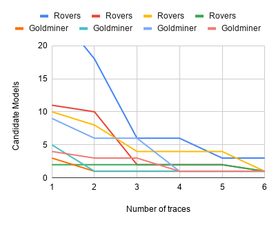
Figure 2: Candidate models VS number of Traces

Fig. 2 shows the variation of the number of candidate models generated with the number of traces. It can clearly be seen that as the number of traces increase, we get fewer but more accurate candidate models.

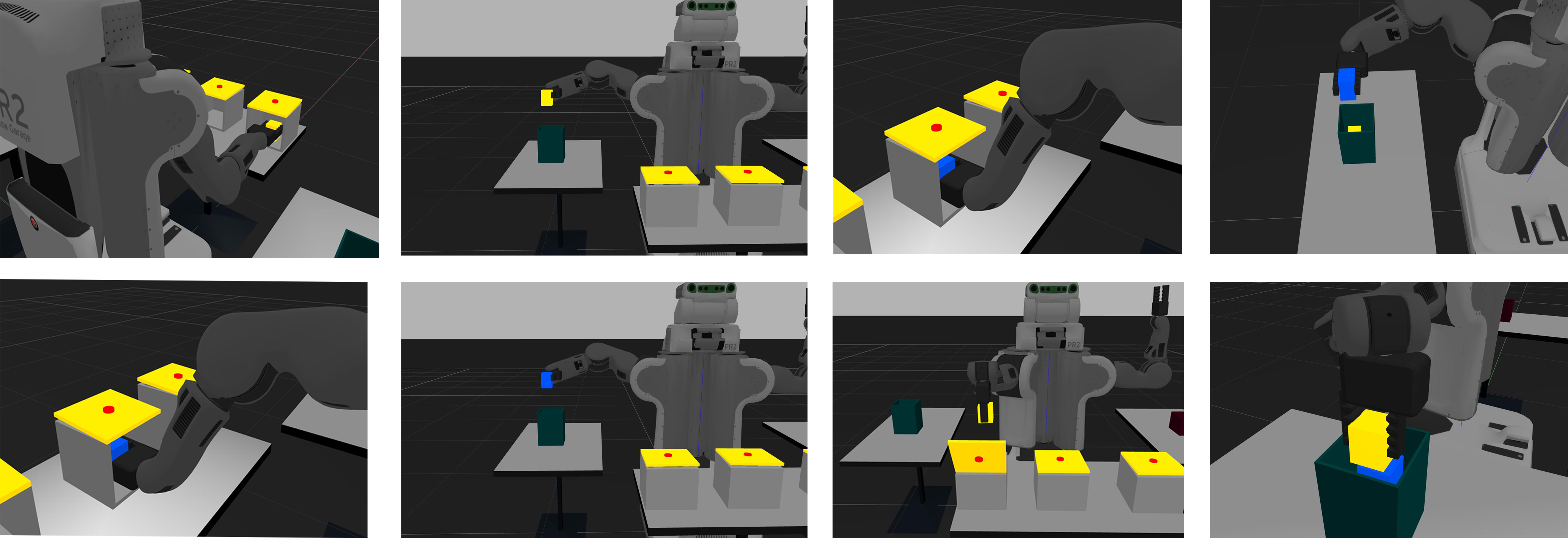
Figure 3: Comparison of action sequence generated with a standard planning method (top) and our method (bottom).

IV-B Simulated Domain

In this experiment, we have created a simulated robotics domain which is a more complex version of our motivating packing domain. In this domain instead of one now we have two constraints for putting items in boxes. As before, the first constraint is that a fragile item cannot be stacked. The second constraint is that a fragile item cannot be dropped into the box and instead it has to be placed carefully. Here, we have two grasping actions: horizontal_grasp and vertical_grasp. For horizontal_grasp, the surroundings of the item to be picked up should be clear. For vertical_grasp, clear surroundings are not a necessity. But in situations where the item to be picked is placed in the container (as shown in Fig. 3), the container needs to be opened first by pressing a button on the top. On the other hand, this is not needed for horizontal_grasp. Furthermore, if the robot has picked up an item horizontally, it is constrained to use drop action instead of place. For vertical grasp, both place and drop are possible. The goal of the robot is the same as before.

Fig. 3 shows the setup of our simulated experiments. The left sequence (top to bottom) is the one that did not use our algorithm. It can be seen that the robot was not able to distinguish between fragile items (in yellow) and non-fragile items (in blue). Hence, it used horizontal_grasp for picking up the fragile item and drop to put the fragile item into the box, which could damage the fragile item. Furthermore, in the subsequent actions, the robot stacked an item over the fragile item, which was also undesirable. On the other hand, in the right sequence showing the actions executed using our algorithms (SS and OS), the robot first picked up the non-fragile item using horizontal_grasp and then put it into the box using the drop action. Then it used vertical_grasp followed by place to stack the fragile item carefully over non-fragile item. This was a successful sequence as none of the constraints of the complete domain were violated. This experiment showed that the robot was able to learn what types of items were not fragile and acted accordingly, with such knowledge completely missing in the domain initially.

V CONCLUSIONS

In this paper, we have formally introduced the problem of Domain Concretization and have discussed its prevalence. We have presented a solution that uses teacher traces and the incomplete domain model to generate a set of candidate models and then finds a robust plan that achieves the goal under the maximum number of candidate models. We have formulated the model search process and developed a sample-based search to make the search more efficient. For practical use, we have also presented an online version of this search method where we used one trace at a time to refine our candidate models. Our methods were tested on IPC domains and a simulated robotics domain where our methods significantly increased plan success rate.

References

- [1] R. S. Sutton and A. G. Barto, Reinforcement Learning: An Introduction. Cambridge, MA, USA: A Bradford Book, 2018.
- [2] A. Y. Ng and S. J. Russell, “Algorithms for inverse reinforcement learning,” in Proceedings of the Seventeenth International Conference on Machine Learning, ser. ICML ’00. San Francisco, CA, USA: Morgan Kaufmann Publishers Inc., 2000, p. 663–670.
- [3] B. D. Ziebart, A. Maas, J. A. Bagnell, and A. K. Dey, “Maximum entropy inverse reinforcement learning,” ser. AAAI’08. AAAI Press, 2008, p. 1433–1438.
- [4] W. Mao and J. Gratch, “A utility-based approach to intention recognition,” in AAMAS 2004, 2004.
- [5] O. Schrempf and U. Hanebeck, “A generic model for estimating user intentions in human-robot cooperation,” in ICINCO, 2005.
- [6] B. Marthi, S. Russell, and J. Wolfe, “Angelic semantics for high-level actions,” in Proceedings of the Seventeenth International Conference on International Conference on Automated Planning and Scheduling, ser. ICAPS’07. AAAI Press, 2007, p. 232–239.
- [7] S. Srivastava, S. Russell, and A. Pinto, “Metaphysics of planning domain descriptions,” in Proceedings of the Thirtieth AAAI Conference on Artificial Intelligence, ser. AAAI’16. AAAI Press, 2016, p. 1074–1080.
- [8] J. J. Finger, “Exploiting constraints in design synthesis,” Ph.D. dissertation, Stanford, CA, USA, 1987.
- [9] J. McCarthy, “Epistemological problems of artificial intelligence,” in Proceedings of the 5th International Joint Conference on Artificial Intelligence - Volume 2, ser. IJCAI’77. San Francisco, CA, USA: Morgan Kaufmann Publishers Inc., 1977, p. 1038–1044.
- [10] M. L. Ginsberg and D. E. Smith, “Reasoning about action ii: The qualification problem,” Artif. Intell., vol. 35, no. 3, p. 311–342, Jul. 1988. [Online]. Available: https://doi.org/10.1016/0004-3702(88)90020-3
- [11] R. E. Fikes and N. J. Nilsson, “Strips: A new approach to the application of theorem proving to problem solving,” Artificial Intelligence, vol. 2, no. 3, pp. 189 – 208, 1971. [Online]. Available: http://www.sciencedirect.com/science/article/pii/0004370271900105
- [12] C. Domshlak and J. Hoffmann, “Probabilistic planning via heuristic forward search and weighted model counting,” J. Artif. Intell. Res. (JAIR), vol. 30, pp. 565–620, 09 2007.
- [13] D. Abel, D. E. Hershkowitz, and M. L. Littman, “Near optimal behavior via approximate state abstraction,” in Proceedings of the 33rd International Conference on International Conference on Machine Learning - Volume 48, ser. ICML’16. JMLR.org, 2016, p. 2915–2923.
- [14] L. P. Kaelbling, M. L. Littman, and A. R. Cassandra, “Planning and acting in partially observable stochastic domains,” Artif. Intell., vol. 101, no. 1–2, p. 99–134, May 1998.
- [15] T. Jaakkola, S. Singh, and M. Jordan, “Reinforcement learning algorithm for partially observable markov decision problems,” Advances in Neural Information Processing Systems, vol. 7, 11 1999.
- [16] S. Kambhampati, “Model-lite planning for the web age masses: The challenges of planning with incomplete and evolving domain models,” in AAAI, 2007.
- [17] C. Weber and D. Bryce, “Planning and acting in incomplete domains,” ser. ICAPS’11. AAAI Press, 2011, p. 274–281.
- [18] T. Nguyen, S. Sreedharan, and S. Kambhampati, “Robust planning with incomplete domain models,” Artificial Intelligence, vol. 245, 01 2017.
- [19] H. Zhuo, T. Nguyen, and S. Kambhampati, “Refining incomplete planning domain models through plan traces,” in IJCAI, 2013.
- [20] H. H. Zhuo, T. Nguyen, and S. Kambhampati, “Model-lite case-based planning,” in Proceedings of the Twenty-Seventh AAAI Conference on Artificial Intelligence, ser. AAAI’13. AAAI Press, 2013, p. 1077–1083.
- [21] Q. Yang, K. Wu, and Y. Jiang, “Learning action models from plan examples using weighted max-sat,” Artificial Intelligence, vol. 171, pp. 107–143, 02 2007.
- [22] H. Zhuo, Q. Yang, D. Hu, and L. Li, “Learning complex action models with quantifiers and logical implications,” Artif. Intell., vol. 174, pp. 1540–1569, 2010.
- [23] H. H. Zhuo and Q. Yang, “Action-model acquisition for planning via transfer learning,” Artificial Intelligence, vol. 212, 07 2014.
- [24] H. H. Zhuo and S. Kambhampati, “Action-model acquisition from noisy plan traces,” in Proceedings of the Twenty-Third International Joint Conference on Artificial Intelligence, ser. IJCAI ’13. AAAI Press, 2013, p. 2444–2450.
- [25] A. Blumer, A. Ehrenfeucht, D. Haussler, and M. K. Warmuth, “Occam’s razor,” Information Processing Letters, vol. 24, no. 6, pp. 377 – 380, 1987. [Online]. Available: http://www.sciencedirect.com/science/article/pii/0020019087901141
- [26] A. Y. Ng and S. J. Russell, “Algorithms for inverse reinforcement learning,” in Proceedings of the Seventeenth International Conference on Machine Learning, ser. ICML ’00. San Francisco, CA, USA: Morgan Kaufmann Publishers Inc., 2000, p. 663–670.
- [27] K. Amin and S. Singh, “Towards resolving unidentifiability in inverse reinforcement learning,” arXiv:1601.06569, 2016.
- [28] S. Armstrong and S. Mindermann, “Occam’s razor is insufficient to infer the preferences of irrational agents,” arXiv:1712.05812, 2017.
- [29] E. Fink and Q. Yang, “Formalizing plan justifications,” 1997. [Online]. Available: https://kilthub.cmu.edu/articles/Formalizing_Plan_Justifications/6605831
- [30] M. Helmert, “The fast downward planning system,” J. Artif. Int. Res., vol. 26, no. 1, p. 191–246, Jul. 2006.