FLAT: Fast, Lightweight and Accurate Method for Cardinality Estimation

Abstract.

Query optimizers rely on accurate cardinality estimation (CardEst) to produce good execution plans. The core problem of CardEst is how to model the rich joint distribution of attributes in an accurate and compact manner. Despite decades of research, existing methods either over-simplify the models only using independent factorization which leads to inaccurate estimates, or over-complicate them by lossless conditional factorization without any independent assumption which results in slow probability computation. In this paper, we propose FLAT, a CardEst method that is simultaneously fast in probability computation, lightweight in model size and accurate in estimation quality. The key idea of FLAT is a novel unsupervised graphical model, called FSPN. It utilizes both independent and conditional factorization to adaptively model different levels of attributes correlations, and thus combines their advantages. FLAT supports efficient online probability computation in near linear time on the underlying FSPN model, provides effective offline model construction and enables incremental model updates. It can estimate cardinality for both single table queries and multi-table join queries. Extensive experimental study demonstrates the superiority of FLAT over existing CardEst methods: FLAT achieves 1–5 orders of magnitude better accuracy, 1–3 orders of magnitude faster probability computation speed and 1–2 orders of magnitude lower storage cost. We also integrate FLAT into Postgres to perform an end-to-end test. It improves the query execution time by $12.9\%$ on the well-known IMDB benchmark workload, which is very close to the optimal result $14.2\%$ using the true cardinality.

PVLDB Reference Format:
Rong Zhu, Ziniu Wu, Yuxing Han, Kai Zeng, Andreas Pfadler, Zhengping Qian, Jingren Zhou, Bin Cui. FLAT: Fast, Lightweight and Accurate Method for Cardinality Estimation. PVLDB, 14(9): 1489 - 1502, 2021.
doi:10.14778/3461535.3461539

1. Introduction

Cardinality estimation (CardEst) is a key component of query optimizers in modern database management systems (DBMS) and analytic engines (Armbrust et al., 2015; Sethi et al., 2019). Its purpose is to estimate the result size of a SQL query before its actual execution, thus playing a central role in generating high-quality query plans.

Given a table $T$ and a query $Q$, estimating the cardinality of $Q$ is equivalent to computing $P$—the probability of records in $T$ satisfying $Q$. Therefore, the core task of CardEst is to condense $T$ into a model $M$ to compute $P$. In general, such models could be obtained in two ways: query-driven and data-driven. Query-driven approaches learn functions mapping a query $Q$ to its predicted probability $P$, so they require large amounts of executed queries as training samples. They only perform well if future queries follow the same distribution as the training workload. Data-driven approaches learn unsupervised models of $\Pr(T)$—the joint probability density function (PDF) of attributes in $T$. As they can generalize to unseen query workload, data-driven approaches receive more attention and are widely used for CardEst.

Challenge and Status of CardEst. An effectual CardEst method should satisfy three criteria (Ioannidis and Christodoulakis, 1991; Tzoumas et al., 2011; Graefe and Mckenna, 1993; Wang et al., 2020), namely high estimation accuracy, fast inference time and lightweight storage overhead, at the same time. Existing methods have made some efforts in finding trade-offs between the them. However, they still suffer from one or more deficiencies when modeling real-world complex data.

In a nutshell, there exist three major strategies for building unsupervised models of $\Pr(T)$ on data table $T$. The first strategy directly compresses and stores all entries in $\Pr(T)$ (Gunopulos et al., 2005; Poosala and Ioannidis, 1997), whose storage overhead is intractable and the lossy compression may significantly impact estimation accuracy. The second strategy utilizes sampling (Leis et al., 2017; Zhao et al., 2018) or kernel density based methods (Kiefer et al., 2017; Heimel et al., 2015), where samples from $T$ are fetched on-the-fly to estimate probabilities. For high-dimensional data, they may be either inaccurate without enough samples or inefficient due to a large sample size.

The third strategy, factorization based methods, is to decompose $\Pr(T)$ into multiple low-dimensional PDFs $\Pr(T^{\prime})$ such that their suitable combination can approximate $\Pr(T)$. However, existing methods often fail to balance the three criteria. Some methods, including deep auto-regression (Yang et al., 2021, 2019; Hasan et al., 2019) and Bayesian Network (Tzoumas et al., 2011; Getoor et al., 2001), can losslessly decompose $\Pr(T)$ using conditional factorization. However, their probability computation speed is reduced drastically. Other methods, such as 1-D histogram (Selinger et al., 1979) and sum-product network (Hilprecht et al., 2019), assume global or local independence between attributes to decompose $\Pr(T)$. They attain high computation efficiency but their estimation accuracy is low when the independence assumption does not hold. We present a detailed analysis of existing data-driven CardEst methods in Section 2.

Our Contributions. In this paper, we address the CardEst problem more comprehensively in order to satisfy all three criteria. We absorb the advantages of existing models and design a novel graphical model, called factorize-sum-split-product network (FSPN). Its key idea to adaptively decompose $\Pr(T)$ according to the dependence level of attributes. Specifically, the joint PDF of highly and weakly correlated attributes will be losslessly separated by conditional factorization and modeled accordingly. The joint PDF of highly correlated attributes can be easily modeled as a multivariate PDF. For the weakly correlated attributes, their joint PDF is split into multiple small regions where attributes are mutually independent in each. We prove that FSPN subsumes 1-D histogram, sum-product network and Bayesian network, and leverages their advantages.

Based on the FSPN model, we propose a CardEst method called FLAT, which is fast, lightweight and accurate. On a single table, FLAT applies an effective offline method for the structure construction of FSPN and an efficient online probability computation method using the FSPN. The probability computation complexity of FLAT is almost linear w.r.t. the number of nodes in FSPN. Moreover, FLAT enables fast incremental updates of the FSPN model.

For multi-table join queries, FLAT uses a new framework, which is more general and applicable than existing work (Hilprecht et al., 2019; Yang et al., 2019; Hasan et al., 2019; Kipf et al., 2019). In the offline phase, FLAT clusters tables into several groups and builds an FSPN for each group. In the online phase, FLAT combines the probabilities of sub-queries in a fast way to get the final result.

In our evaluation, FLAT achieves state-of-the-art performance on both single table and multi-table cases in comparison with all existing methods (Kipf et al., 2019; Yang and Wu, 2019; Yang et al., 2021; Hilprecht et al., 2019; Tzoumas et al., 2011; Poosala and Ioannidis, 1997; Kiefer et al., 2017; Leis et al., 2017). On single table, FLAT achieves up to $1$–$5$ orders of magnitude better accuracy, $1$–$3$ orders of magnitude faster probability computation speed (near $0.2ms$) and $1$–$2$ orders of magnitude lower storage cost (only tens of KB). On the JOB-light benchmark (Leis et al., 2018, 2015) and a more complex crafted multi-table workload, FLAT also attains the highest accuracy and an order of magnitude faster computation time (near $5ms$), while requiring only $3.3$MB storage space. We also integrate FLAT into Postgres. It improves the average end-to-end query time by $12.9\%$ on the benchmark workload, which is very close to the optimal result $14.2\%$ using the true cardinality. This result confirms with a positive answer to the long-existing question whether and how much a more accurate CardEst can improve the query plan quality (Perron et al., 2019). In addition, we have deployed FLAT in the production environment of our company. We also plan to release to the community an open-source implementation of FLAT.

In summary, our main contributions are listed as follows:

1) We analyze in detail the status of existing data-driven CardEst methods in terms of the above three criteria (in Section 2).

2) We present FSPN, a novel unsupervised graphical model, which combines the advantages of existing methods in an adaptive manner (in Section 3).

3) We propose FLAT, a CardEst method with fast probability computation, high estimation accuracy and low storage cost, on both single table and multi-table join queries (in Section 4 and 5).

4) We conduct extensive experiments and end-to-end test on Postgres to demonstrate the superiority and practicality of our proposed methods (in Section 6).

2. Problem Definition and Background

In this section, we formally define the CardEst problem and analyze the status of data-driven CardEst methods. Based on the analysis, we summarize some key findings that inspire our work.

CardEst Problem. Let $T$ be a table with a set of $k$ attributes $A=\{A_{1},A_{2},\dots,A_{k}\}$. $T$ could either be a single or a joined table. Each attribute $A_{i}$ in $T$ is assumed to be either categorical, so that values can be mapped to integers, or continuous. Without loss of generality, we assume that the domain of $A_{i}$ is $[LB_{i},UB_{i}]$.

In this paper, we do not consider “LIKE” queries on strings. Any selection query $Q$ on $T$ may be represented in canonical form: $Q=(A_{1}\in[L_{1},U_{1}]\wedge A_{2}\in[L_{2},U_{2}]\wedge\cdots\wedge A_{k}\in[L_{k},U_{k}])$, where $LB_{i}\leq L_{i}\leq U_{i}\leq UB_{i}$ for all $i$. W.l.o.g., the endpoints of each interval can also be open. We call $Q$ a point query if $L_{i}=U_{i}$ for all $i$ and range query otherwise. If $Q$ has no constraint on the left or right hand side of $A_{i}$, we simply set $L_{i}=LB_{i}$ or $U_{i}=UB_{i}$, respectively. For any query $Q^{\prime}$ where the constraint of an attribute $A_{i}$ contains several intervals, we may split $Q^{\prime}$ into multiple queries satisfying the above form.

Let $\textsf{Card}(T,Q)$ denote the exact number of records in $T$ satisfying all predicates in $Q$. Generally, the CardEst problem asks to estimate the value of $\textsf{Card}(T,Q)$ as accurately as possible without executing $Q$ on $T$. CardEst is often modeled and solved from a statistical perspective. We can regard each attribute $A_{i}$ in $T$ as a random variable. The table $T$ essentially represents a set of i.i.d. records sampled from the joint PDF $\Pr_{\textit{{t}}}(A)=\Pr_{\textit{{t}}}(A_{1},A_{2},\dots,A_{k})$. For any query $Q$, let $\Pr_{\textit{{t}}}(Q)$ denote the probability of records in $T$ satisfying $Q$. We have $\textsf{Card}(T,Q)=\Pr\nolimits_{\textit{{t}}}(Q)\cdot|T|$. Therefore, estimating $\textsf{Card}(T,Q)$ is equivalent to estimating the probability $\Pr_{\textit{{t}}}(Q)$. Unsupervised CardEst solves this problem in a purely data-driven fashion, which can be formally stated as follows:

Offline Training: Given a table $T$ with a set $A$ of attributes as input, output a model $\widehat{\Pr}_{\textit{{t}}}(A)$ for $\Pr_{\textit{{t}}}(A)$ such that $\widehat{\Pr}_{\textit{{t}}}(A)\approx\Pr_{\textit{{t}}}(A)$.

Online Probability Computation: Given the model $\widehat{\Pr}_{\textit{{t}}}(A)$ and a query $Q$ as input, output $\widehat{\Pr}_{\textit{{t}}}(Q)\cdot|T|$ as the estimated cardinality.

Data-Driven CardEst Methods Analysis. We use three criteria, namely model accuracy, probability computation speed and storage overhead, to analyze existing methods. The results are as follows:

1) Lossy FullStore (Gunopulos et al., 2005) stores all entries in $\Pr_{\textit{{t}}}(A)$ using compression techniques, whose storage grows exponentially in the number of attributes and becomes intractable (Yang et al., 2019, 2021).

2) Sample and Kernel-based methods (Leis et al., 2017; Zhao et al., 2018; Kiefer et al., 2017; Heimel et al., 2015) do not store $\Pr_{\textit{{t}}}(A)$ but rather sample records from $T$ on-the-fly, or use average kernels centered around sampled points to estimate $\Pr_{\textit{{t}}}(Q)$. For high-dimensional data, they may be either inaccurate without enough samples, or inefficient due to a large sample size.

Alternatively, a more promising way is to factorize $\Pr_{\textit{{t}}}(A)$ into multiple low-dimensional PDFs $\Pr_{\textit{{t}}}(A^{\prime})$ such that: 1) $|A^{\prime}|<<|A|$ so $\Pr_{\textit{{t}}}(A^{\prime})$ is easier to store and model; and 2) a suitable combination, e.g. multiplication, weighted sum and etc, of $\Pr_{\textit{{t}}}(A^{\prime})$ approximates $\Pr_{\textit{{t}}}(A)$. Some representative methods are listed in the following:

3) 1-D Histogram (Selinger et al., 1979) assumes all attributes are mutually independent, so that $\widehat{\Pr}_{\textit{{t}}}(A)=\prod_{i=1}^{k}\widehat{\Pr}_{\textit{{t}}}(A_{i})$. Each $\widehat{\Pr}_{\textit{{t}}}(A_{i})$ is built as a (cumulative) histogram, so $\widehat{\Pr}_{\textit{{t}}}(Q)$ may be obtained in $O(|A|)$ time. However, the estimation errors may be high, since correlations between attributes are ignored.

4) M-D Histogram  (Poosala and Ioannidis, 1997; Deshpande et al., 2001; Gunopulos et al., 2000; Wang and Sevcik, 2003) builds multi-dimensional histograms to model the dependency of attributes. They identify subsets of correlated attributes using models such as Markov network, build histograms on each subset and assume the independence across different subsets. It improves the accuracy but the decomposition is still lossy. Meanwhile, it is space consuming.
5) Deep Auto-Regression (DAR) (Yang et al., 2021, 2019; Hasan et al., 2019) decomposes the joint PDF according to the chain rule, i.e., $\Pr_{\textit{{t}}}(A)\!=\!\Pr_{\textit{{t}}}(A_{1})\cdot\prod_{i=2}^{k}\!\Pr_{\textit{{t}}}(A_{i}|\break A_{1},A_{2},\dots,A_{i-1})$. Each conditional PDF can be parametrically modeled by a deep neural network (DNN). While the expressiveness of DNNs allows $\Pr_{\textit{{t}}}(A)$ to be approximated well, probability computation time and space cost increase with the width and depth of the DNN. Moreover, for range query $Q$, computing $\Pr_{\textit{{t}}}(Q)$ requires averaging the probabilities of lots of sample points in the range. Thus, the probability computation on DAR is relatively slow.
6) Bayesian Network (BN)  (Tzoumas et al., 2011; Getoor et al., 2001; Chow and Liu, 1968) models the dependence structure between all attributes as a directed acyclic graph and assumes that each attribute is conditionally independent of the remaining attributes given its parents. The probability $\Pr_{\textit{{t}}}(A)$ is factorized as $\Pr_{\textit{{t}}}(A)=\prod_{i=1}^{k}\Pr_{\textit{{t}}}(A_{i}|A_{\text{pa}(i)})$, where $\text{pa}(i)$ is the parent attributes of $A_{i}$ in BN. Learning the BN structure from data and probability computation on BN are both NP-hard (Scanagatta et al., 2019; Dagum and Luby, 1993).
7) Sum-Product Network (SPN) (Hilprecht et al., 2019) approximates $\Pr_{\textit{{t}}}(A)$ using several local and simple PDFs. An SPN is tree structure where each node stands for an estimated PDF $\widehat{\Pr}_{\textit{{t}}^{\prime}}(A^{\prime})$ of the attribute subset $A^{\prime}$ on record subset $T^{\prime}\subseteq T$ (Poon and Domingos, 2011). The root node represents $\widehat{\Pr}_{\textit{{t}}}(A)$. Each inner node is: 1) a sum node which splits all records (rows) in $T^{\prime}$ into $T_{i}^{\prime}$ on each child such that $\widehat{\Pr}_{\textit{{t}}^{\prime}}(A^{\prime})=\sum_{i}w_{i}\widehat{\Pr}_{\textit{{t}}_{i}^{\prime}}(A^{\prime})$ with weights $w_{i}$; or 2) a product node which splits attributes (columns) in $A^{\prime}$ on each child as $\widehat{\Pr}_{\textit{{t}}^{\prime}}(A^{\prime})=\prod_{j}\widehat{\Pr}_{\textit{{t}}^{\prime}}(A_{j}^{\prime})$ when all $A_{j}^{\prime}$ are mutually independent in $T^{\prime}$. Each leaf node then maintains a (cumulative) PDF on a singleton attribute. The probability $\widehat{\Pr}_{\textit{{t}}}(Q)$ can be computed in a bottom-up manner using the SPN node operations for both point and range queries. The storage overhead and probability computation cost are linear in the number of nodes of SPN.

The performance of SPN heavily relies on the local independence assumption. When it holds, the generated SPN is compact and exhibits superiority over other methods (Hilprecht et al., 2019; Yang et al., 2021). However, real-world data often possesses substantial skew and strong correlations between attributes (Tzoumas et al., 2011). In this situation, SPN can not split these attributes using the product operation and might repeatedly apply the sum operation to split records into extremely small volumes (Martens and Medabalimi, 2014), i.e., $|T^{\prime}|=1$. This would heavily increase the SPN size, degrade its efficiency and make the model inaccurate (Desana and Schnörr, 2020; Martens and Medabalimi, 2014).

Inspirations. Based on the analysis, there does not exist a comprehensively effectual CardEst method since each method only utilizes one factorization approach. However, independent factorization has low storage cost and supports fast inference but may incur huge estimation errors; conditional factorization can accurately decompose the PDF but the inference is costly. This leads to our key question: if we could, in an adaptive manner, apply both kinds of factorization, would it be possible to obtain a CardEst method that can simultaneously satisfy all three criteria? We answer this question affirmatively with a new unsupervised model, called factorize-split-sum-product network (FSPN), which integrates the strength of both factorization approaches.

3. The FSPN Model

In this section, we present FSPN, a new tree-structured graphical model representing the joint PDF of a set of attributes in an adaptive manner. We first explain the key ideas of FSPN with an example and then present its formal definition. Finally, we compare FSPN with aforementioned models.

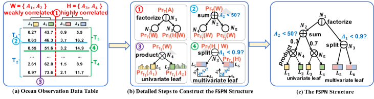
Figure 1. An ocean observation data table and its corresponding FSPN.

Key Ideas of FSPN. FSPN can factorize attributes with different dependence levels accordingly. The conditional factorization approach is used to split highly and weakly correlated attributes. Then, highly correlated attributes are directly modeled together while weakly correlated attributes are recursively approximated using the independent factorization approach. Figure 1(a) gives an example of table $T$ with a set $A$ of four attributes water turbidity ($A_{1}$), temperature ($A_{2}$), wave height ($A_{3}$) and wind force ($A_{4}$). We elaborate the process to construct its FSPN in Figure 1(b) as follows:

At first, we examine the correlations between each pair of attributes in $T$. $A_{3}$ and $A_{4}$ are globally highly correlated, so they can not be decomposed as independent attributes unless we split $T$ into extremely small clusters as SPN. Instead, we can losslessly separate them from other attributes as early as possible and process each part respectively. Let $H=\{A_{3},A_{4}\}$ and $W=\{A_{1},A_{2}\}$. We apply the conditional factorization approach and factorize $\Pr_{\textit{{t}}}(A)=\Pr_{\textit{{t}}}(W)\cdot\Pr_{\textit{{t}}}(H|W)$ (as node $N_{1}$ in step ①). $\Pr_{\textit{{t}}}(W)$ and $\Pr_{\textit{{t}}}(H|W)$ are then modeled in different ways.

The two attributes $A_{1}$ and $A_{2}$ in $W$ are not independent on $T$ but they are weakly correlated. Thus, we can utilize the independent factorization approach on small subsets of $T$. In our example, if we split all records in $T$ into $T_{1}$ and $T_{2}$ based on whether $A_{1}$ is less than $50$ (as node $N_{2}$ in step ②), $A_{1}$ and $A_{2}$ are independent on both $T_{1}$ and $T_{2}$. This situation is called contextually independent, where $T_{1}$ and $T_{2}$ refer to the specific context. Since $\Pr_{\textit{{t}}_{1}}(W)=\Pr_{\textit{{t}}_{1}}(A_{1})\cdot\Pr_{\textit{{t}}_{1}}(A_{2})$ (as node $N_{4}$ in step ③), we then simply use two univariate PDFs (such as histograms in leaf nodes $L_{1}$ and $L_{2}$ in step ③) to model $\Pr_{\textit{{t}}_{1}}(A_{1})$ and $\Pr_{\textit{{t}}_{1}}(A_{2})$ on $T_{1}$, respectively. Similarly, we also model $\Pr_{\textit{{t}}_{2}}(W)=\Pr_{\textit{{t}}_{2}}(A_{1})\cdot\Pr_{\textit{{t}}_{2}}(A_{2})$ on $T_{2}$ (as node $N_{5}$).

For the conditional PDF $\Pr_{\textit{{t}}}(H|W)$, we do not need to specify $\Pr(H|w)$ for each value $w$ of $W$. Instead, we can recursively split $T$ into multiple regions $T_{j}$ in terms of $W$ such that $H$ is independent of $W$ in each context $T_{j}$, i.e., $\Pr_{\textit{{t}}_{j}}(H)=\Pr_{\textit{{t}}_{j}}(H|W)$. At this time, for any value $w$ of $W$ falling in the same region, $\Pr_{\textit{{t}}_{j}}(H|w)$ stays the same, so we only need to maintain $\Pr_{\textit{{t}}_{j}}(H)$ for each region. We refer to this situation as contextual condition removal. In our example, we split $T$ into $T_{3}$ and $T_{4}$ (as nodes $N_{3}$ in step ④) by whether the condition attribute $A_{1}$ is less than $0.9$. $W$ is independent of $H$ on each leaf node region, so we only need to model $\Pr_{\textit{{t}}_{3}}(H)$ and $\Pr_{\textit{{t}}_{4}}(H)$. Thus, we model them as two multivariate leaf nodes $L_{5}$ and $L_{6}$ in step ④. Note that, attribute values in $H$ are interdependent and their joint PDFs $\Pr_{\textit{{t}}_{3}}(H)$ and $\Pr_{\textit{{t}}_{4}}(H)$ are sparse in the two-dimensional space, so they are easy modeled as a multivariate PDF.

Finally, we obtain an FSPN in Figure 1(c) containing 11 nodes, where 5 inner nodes represent different operations to split data and 6 leaf nodes keep PDFs for different parts of the original data.

Formulation of FSPN. Let $\mathcal{F}$ denote a FSPN modeling the joint PDF $\Pr_{\textit{{t}}}(A)$ for records $T$ with attributes $A$. $\mathcal{F}$ is a tree structure. Each node $N$ in $\mathcal{F}$ is a 4-tuple $(A_{\textit{{n}}},C_{\textit{{n}}},T_{\textit{{n}}},O_{\textit{{n}}})$ where:

$\bullet$ $T_{\textit{{n}}}\subseteq T$ represents a set of records where the PDF is built on. It is called the context of node $N$.

$\bullet$ $A_{\textit{{n}}},C_{\textit{{n}}}\subseteq A$ represent two set of attributes. We call $A_{\textit{{n}}}$ and $C_{\textit{{n}}}$ the scope and condition of node $N$, respectively. If $C_{\textit{{n}}}=\emptyset$, $N$ represents the PDF $\Pr_{\textit{{t}}_{\textit{{n}}}}(A_{\textit{{n}}})$; otherwise, it represents the conditional PDF $\Pr_{\textit{{t}}_{\textit{{n}}}}(A_{\textit{{n}}}|C_{\textit{{n}}})$. The root of $\mathcal{F}$, such as $N_{1}$ in Figure 1(c), is a node with $A_{\textit{{n}}}=A$, $C_{\textit{{n}}}=\emptyset$ and $T_{\textit{{n}}}=T$ representing the joint PDF $\Pr_{\textit{{t}}}(A)$.

$\bullet$ $O_{\textit{{n}}}$ stands for the operation specifying how to split data to generate its children in different ways:
1) A Factorize ($|$⃝) node, such as $N_{1}$ in step ①, splits highly correlated attributes from the remaining ones by conditional factorization only when $C_{\textit{{n}}}=\emptyset$. Let $H\subseteq A_{\textit{{n}}}$ be a subset of highly correlated attributes. It generates the left child $N_{\textit{{l}}}=(A_{\textit{{n}}}-H,\emptyset,T_{\textit{{n}}},O_{\textit{{l}}})$ and the right child $N_{\textit{{r}}}=(H,A_{\textit{{n}}}-H,T_{\textit{{n}}},O_{\textit{{r}}})$. We have $\Pr_{\textit{{t}}_{\textit{{n}}}}(A_{\textit{{n}}})=\Pr_{\textit{{t}}_{\textit{{n}}}}(A_{\textit{{n}}}-H)\cdot\Pr_{\textit{{t}}_{\textit{{n}}}}(H|A_{\textit{{n}}}-H)$.
2) A Sum ($+$⃝) node, such as $N_{2}$ in step ②, splits the records in $T_{\textit{{n}}}$ in order to enforce contextual independence only when $C_{\textit{{n}}}=\emptyset$. We partition $T_{\textit{{n}}}$ into subsets $T_{1},T_{2},\dots,T_{n}$. For each $1\leq i\leq n$, $N$ generates the child $N_{i}=(A_{\textit{{n}}},\emptyset,T_{i},O_{i})$ with weight $w_{i}=|T_{i}|/|T_{\textit{{n}}}|$. We can regard $N$ as a mixture of models on all of its children, i.e., $\Pr_{\textit{{t}}_{\textit{{n}}}}(A_{\textit{{n}}})=\sum_{i=1}^{n}w_{i}\Pr_{\textit{{t}}_{i}}(A_{\textit{{n}}})$, where $w_{i}$ represents the proportion of the $i$-th subset.
3) A Product ($\times$⃝) node, such as $N_{4}$ in step ③, splits the scope $A_{\textit{{n}}}$ of $N$ only when $C_{\textit{{n}}}=\emptyset$ and contextual independence holds. Let $A_{1},A_{2},\dots,A_{m}$ be the mutually independent partitions of $A_{\textit{{n}}}$. $N$ generates children $N_{j}=(A_{j},\emptyset,T_{\textit{{n}}},O_{j})$ for all $1\leq j\leq m$ such that $\Pr_{\textit{{t}}_{\textit{{n}}}}(A_{\textit{{n}}})=\prod_{j=1}^{m}\Pr_{\textit{{t}}_{\textit{{n}}}}(A_{j})$.
4) A Split ($-$⃝) node, such as $N_{3}$ in step ④, partitions the records $T_{\textit{{n}}}$ into disjoint subsets $T_{1},T_{2},\dots,T_{d}$ only when $C_{\textit{{n}}}\neq\emptyset$. For each $1\leq i\leq d$, $N$ generates the child $N_{i}=(A_{\textit{{n}}},C_{\textit{{n}}},T_{i},O_{i})$. Note that for any value $c$ of $C_{\textit{{n}}}$, there exists exactly one $j$ such that $c$ falls in the region of $T_{j}$. The semantic of split is different from sum. The split node divides a large model of $\Pr_{T_{\textit{{n}}}}(A_{\textit{{n}}}|C_{\textit{{n}}})$ into several parts by the values of $C_{\textit{{n}}}$. Whereas, the sum node decomposes a large model of $\Pr_{T_{\textit{{n}}}}(A_{\textit{{n}}})$ to small models on the space of $A_{\textit{{n}}}$.
5) A Uni-leaf ($\square$) node, such as $L_{1}$ and $L_{2}$ in step ③, keeps the univariate PDF $\Pr_{T_{\textit{{n}}}}(A_{\textit{{n}}})$, such as histogram or Gaussian mixture model, only when $|A_{\textit{{n}}}|=1$ and $C_{\textit{{n}}}=\emptyset$.
6) A Multi-leaf ($\square\!\square$) node, such as $L_{5}$ and $L_{6}$ in step ④, maintains the multivariate PDF $\Pr_{T_{\textit{{n}}}}(A_{\textit{{n}}})$ only when $C_{\textit{{n}}}\neq\emptyset$ and $A_{\textit{{n}}}$ is independent of $C_{\textit{{n}}}$ on $T_{\textit{{n}}}$.

The above operations are recursively used to construct $\mathcal{F}$ with three constraints: 1) for a factorize node, the right child must be a split node or multi-leaf; the left child can be any type in sum, product, factorize and uni-leaf; 2) the children of a sum or product node could be any type in sum, product, factorize and uni-leaf; and 3) the children of a split node can only be split or multi-leaf nodes.

Differences with SPN. As the name suggests, FSPN is inspired by SPN and its successful application in CardEst  (Hilprecht et al., 2019). However, FSPN differs from SPN in two fundamental aspects. First, in terms of the underlying key ideas, FSPN tries to adaptively model attributes with different levels of dependency, which is not considered in SPN. Second, in terms of the fundamental design choices, FSPN can split weakly and highly correlated attributes, and models each class differently: 1) weakly correlated attributes are modeled by sum and product operations; and 2) for highly correlated attributes, FSPN uses split and multi-leaf nodes. SPN only uses the first technique on all attributes. As per our analysis in Section 2, this can generate a large structure since local independence can not easily hold.

Moreover, a simple extension of SPN with multi-leaf nodes also seems unlikely to mitigate its inherent limitations. This is because multi-leaf nodes can only efficiently model highly correlated attributes, as their joint PDF can be easily reduced to and modeled in a low dimensional space. Otherwise, their storage cost grows exponentially so the model size would be very large. FSPN guarantees that multi-leaf nodes are only applied on highly correlated attributes, whereas SPN and its extensions lack such mechanism. Our experimental results in Section 6.1 exhibit that the model size of SPN with multi-leaf nodes are much larger than FSPN and may exceed the memory limit on highly correlated table.

Generality of FSPN. We show that FSPN generalizes 1-D Histogram, SPN and BN models. First, when all attributes are mutually independent, FSPN becomes 1-D Histogram. Second, FSPN degenerates to SPN by disabling the factorize operation. Third, FSPN could equally represent a BN model on discrete attributes by iteratively factorizing each attribute having no parents from others. We put the transformation process in Appendix A.1. Based on it, we obtain Lemma 1 (proved in Appendix A.2) stating that the FSPN is no worse than SPN and BN in terms of expressive efficiency.

Lemma 1 Given a table $T$ with attributes $A$, if the joint PDF $\Pr_{\textit{{t}}}(A)$ is represented by an SPN $\mathcal{S}$ or a BN $\mathcal{B}$ with space cost $O(M)$, then there exists an FSPN $\mathcal{F}$ that can equivalently model $\Pr_{\textit{{t}}}(A)$ with no more than $O(M)$ space.

4. Single Table CardEst Method

In this section, we propose FLAT, a fast, lightweight and accurate CardEst algorithm built on FSPN. We first introduce how FLAT computes the probability on FSPN online in Section 4.1. Then, we show how FLAT constructs the FSPN from data offline in Section 4.2. Finally, we discuss how FLAT updates the model in Section 4.3.

4.1. Online Probability Computation

FLAT can obtain the probability (cardinality) of any query $Q$ in a recursive manner on FSPN. We first show the basic strategy of probability computation with an example, and then present the detailed algorithm and analyze its complexity.

Basic Strategy. As stated in Section 2, the query $Q$ can be represented in canonical form: $Q=(A_{1}\in[L_{1},U_{1}]\wedge A_{2}\in[L_{2},U_{2}]\wedge\cdots\wedge\break A_{k}\in[L_{k},U_{k}])$, where $L_{i}\leq A_{i}\leq U_{i}$ is the constraint on attribute $A_{i}$. Obviously, $Q$ represents a hyper-rectangle range in the attribute space whose probability needs to be computed. In Figure 2, we give an example query $Q$ on the FSPN in Figure 1(c).

First, considering the root node $N_{1}$, computing the probability of $Q$ on this factorize node is a non-trivial task. For each point $r\in Q$, we can obtain its probability $\Pr_{r}(A_{1},A_{2})$ from node $N_{2}$ and the conditional probability $\Pr_{r}(A_{3},A_{4}|A_{1},A_{2})$ from node $N_{3}$. However, for different $r$, $\Pr_{r}(A_{3},A_{4}|A_{1},A_{2})$ is modeled by different PDFs on multi-leaf nodes $L_{5}$ or $L_{6}$ of $N_{3}$. Thus, we must split $Q$ into two regions to compute the probability of $Q$ (as step ① in Figure 2). To this end, we push $Q$ onto $N_{3}$, whose splitting rule on the condition attributes ($A_{1}<0.9$) would divide $Q$ into two hyper-rectangle ranges $Q_{1}$ and $Q_{2}$ on multi-leaf nodes $L_{5}$ or $L_{6}$, respectively. For $Q_{1}$ (or $Q_{2}$), the probability $\Pr(A_{3},A_{4}|A_{1},A_{2})=\Pr(A_{3},A_{4})$ can be directly obtained from the multivariate PDF on $L_{5}$ (or $L_{6}$).

Then, we can compute the probability $\Pr(A_{1},A_{2})$ for each region $Q_{1}$ and $Q_{2}$ from $N_{2}$. Obviously, for the sum node (e.g. $N_{2}$) and product node (e.g. $N_{4}$), the probability of each region can be recursively obtained by summing (as step ③) or multiplying (as step ②) the probability values of its children, respectively. In the base case, the probability on the singleton attribute $A_{1}$ (or $A_{2}$) is obtained from the uni-leaf nodes $L_{1}$ and $L_{3}$ (or $L_{2}$ and $L_{4}$). Finally, since $\Pr(A_{1},A_{2})$ and $\Pr(A_{3},A_{4})$ are independent in $Q_{1}$ and $Q_{2}$, we can multiply and sum them together ((as step ④)) to obtain the probability of $Q$.

Algorithm Description. Next, we describe the online probability computation algorithm FLAT-Online. It takes as inputs a FSPN $\mathcal{F}$ modeling $\Pr_{\textit{{t}}}(A)$ and the query $Q$, and outputs $\Pr_{\textit{{t}}}(Q)$ on $\mathcal{F}$. Let $N$ be the root node of $\mathcal{F}$ (line 1). For any node $N^{\prime}$ in $\mathcal{F}$, let $\mathcal{F}_{\textit{{n}}^{\prime}}$ denote the FSPN rooted at $N^{\prime}$. FLAT-Online recursively computes the probability of $Q$ by the following rules:

Rule 1 (lines 2–3): Basically, if $N$ is a uni-leaf node, we directly return the probability of $Q$ on the univariate PDF of the attribute.

Rule 2 (lines 4–11): if $N$ is a sum node (lines 4–7) or a product node (lines 8–11), let $N_{1},N_{2},\dots,N_{t}$ be all of its children. We can further call FLAT-Online on $\mathcal{F}_{\textit{{n}}_{i}}$ for each $1\leq i\leq t$ to obtain the probability on the PDF represented by each child. Then, node $N$ computes a weighted sum (for sum node) or multiplication (for product node) of these probabilities.

Rule 3 (lines 12–18): if $N$ is a factorize node, let $LC$ and $RC$ be its left and right child modeling $\Pr_{\textit{{t}}}(W)$ and $\Pr_{\textit{{t}}}(H|W)$, respectively. All descendants of $RC$ are split or multi-leaf nodes. Let $L_{1},L_{2},\dots,L_{t}$ be all multi-leaf descendants of $RC$. We assume that each split node divides the attribute domain space in a grid manner, which is ensured by the FSPN structure construction method in Section 4.2. Then, each $L_{i}$ maintains a multivariate PDF on a hyper-rectangle range specified by all split nodes on the path from $RC$ to $L_{i}$. Based on these ranges, we can divide the range of query $Q$ into $Q_{1},Q_{2},\dots,Q_{t}$. For each $Q_{i}$, the probability $h_{i}$ on highly correlated attributes $H$ could be directly obtained from $L_{i}$. The probability $w_{i}$ on attributes $W$ could be recursively obtained by calling FLAT-Online on $\mathcal{F}_{\textit{{l}}\textit{{c}}}$, the FSPN rooted at $LC$, and $Q_{i}$. After that, since $H$ is independent of $W$ on the range of each $Q_{i}$, we sum all products $h_{i}w_{i}$ together as the probability of $Q$.

Range	$A_{1}$ $\blacksquare$	$A_{2}$ $\blacksquare$	$A_{3}$ $\blacksquare$	$A_{4}$ $\blacksquare$
Bound	[0, 10]	[0, 100]	[0, 100]	[0, 100]
Leaf $L_{5}$	[0, 0.9)	[0, 100]	[0, 100]	[0, 100]
Leaf $L_{6}$	[0.9, 10]	[0, 100]	[0, 100]	[0, 100
Query $Q$	[0.6, 1.4]	[35, 65]	[2, 3]	[60, 70]
Query $Q_{1}$	[0.6, 0.9)	[35, 65]	[2, 3]	[60, 70]
Query $Q_{2}$	[0.9, 1.4]	[35, 65]	[2, 3]	[60, 70]

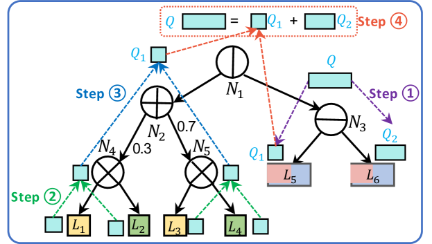
Figure 2. An example of the FLAT probability computation.

 

    Algorithm FLAT-Online$(\mathcal{F},Q)$

1: let $N$ be the root node of $\mathcal{F}$

2: if $N$ is uni-leaf node then

3:    return  $\Pr_{\textit{{t}}}(Q)$ by the univariate PDF on the attribute modeled by $N$

4: else if $N$ is a sum node then

5:    let $N_{1},N_{2},\dots,N_{t}$ be the children of $N$ with weights $w_{1},w_{2},\dots,w_{t}$

6:    $p_{i}\leftarrow\textsf{FLAT-Online}(\mathcal{F}_{\textit{{n}}_{i}},Q)$ for each $1\leq i\leq t$

7:    return  $\sum_{i=1}^{t}w_{i}p_{i}$

8: else if $N$ is a product node then

9:    let $N_{1},N_{2},\dots,N_{t}$ be the children of $N$

10:    $p_{i}\leftarrow\textsf{FLAT-Online}(\mathcal{F}_{\textit{{n}}_{i}},Q)$ for each $1\leq i\leq t$

11:    return  $\prod_{i=1}^{t}p_{i}$

12: else

13:    let $LC$ be the left child modeling $\Pr_{\textit{{t}}}(W)$ and $RC$ be the right child modeling $\Pr_{\textit{{t}}}(H|W)$

14:    let $L_{1},L_{2},\dots,L_{t}$ be all the multi-leaf descendants of $RC$

15:    split $Q$ into $Q_{1},Q_{2},\dots,Q_{t}$ by ranges of $L_{1},L_{2},\dots,L_{t}$

16:    get $h_{i}$ of $Q_{i}$ on variables $H$ from the multivariate PDF on $L_{i}$ for each $1\leq i\leq t$

17:    $w_{i}\leftarrow\textsf{FLAT-Online}(\mathcal{F}_{\textit{{l}}\textit{{c}}},Q_{i})$ for each $1\leq i\leq t$

18:    return  $\sum_{i=1}^{t}h_{i}w_{i}$

 

Complexity Analysis. We assume that, on each leaf node, the probability of any range can be computed in $O(1)$ time, which can be easily implemented by a cumulative histogram or Gaussian mixture functions. Let $n$ be the number of nodes in FSPN. Let $f$ and $m$ be the number of factorize and multi-leaf nodes in FSPN, respectively. The maximum number of ranges to be computed on each node is $O(m^{f})$, so the time cost of FLAT-Online is $O(m^{f}n)$.

By our empirical testing, the actual time cost of FLAT-Online is almost linear w.r.t. the number of nodes in FSPN for two reasons. First, FSPN is compact on real-world data so both $f$ and $n$ are small. Second, the computation on many ranges in each node could be easily done in parallel. In our testing, the speed of FLAT-Online is even near the histogram method and $1$–$3$ orders of magnitude faster than other methods (See Section 6.1).

4.2. Offline Structure Construction

We present the detailed procedures to build an FSPN in the algorithm FLAT-Offline. Its general process is shown in Figure 3. FLAT-Offline works in a top-down manner. Each node $N$ takes the scope attributes $A_{\textit{{n}}}$, the condition attributes $C_{\textit{{n}}}$ and the context of records $T_{\textit{{n}}}$ as inputs, and recursively decompose the joint PDF to build the FSPN rooted at $N$. To build the FSPN $\mathcal{F}$ modeling table $T$ with attributes $A$, we can directly call $\textsf{FLAT-Offline}(A,\emptyset,T)$. We briefly scan its main procedures as follows:

1. Separating highly correlated attributes with others (lines 2–8): when $C_{\textit{{n}}}=\emptyset$, FLAT-Offline firstly detects if there exists a set $H$ of highly correlated attributes since the principle of FSPN is to separate them with others as early as possible (step ① in Figure 3). We find $H$ by examining pairwise correlations, e.g. RDC (Lopez-Paz et al., 2013), between attributes and iteratively group attributes whose correlation value is larger than a threshold $\tau_{h}$. If $H\neq\emptyset$, we set $N$ to be a factorize node. The left child and right child of $N$ recursively call FLAT-Offline to model $\Pr_{\textit{{t}}_{\textit{{n}}}}(A_{\textit{{n}}}-H)$ and $\Pr_{T_{\textit{{n}}}}(H|A_{\textit{{n}}}-H)$, respectively.

2. Modeling weakly correlated attributes (lines 9–19): if $C_{\textit{{n}}}=\emptyset$ and $H=\emptyset$, we try to split $\Pr_{\textit{{t}}_{\textit{{n}}}}(A_{\textit{{n}}})$ into small regions such that attributes in $A_{\textit{{n}}}$ are locally independent. Specifically, if $|A_{\textit{{n}}}|=1$, $N$ is a uni-leaf node (line 10). We call the Leaf-PDF procedure to model univariate PDF $\Pr_{\textit{{t}}_{\textit{{n}}}}(A_{\textit{{n}}})$ (line 11) using off-the-shelf tools. In our implementation, we choose histograms (Poosala and Ioannidis, 1997) and parametric Gaussian mixture functions (Rasmussen, 2000) to model categorical and continuous attributes, respectively.

Otherwise, we try to partition $A_{\textit{{n}}}$ into mutually independent subsets based on their pairwise correlations (step ② in Figure 3). Two attributes are regarded as independent if their correlation value is no larger than than a threshold $\tau_{l}$. If $A_{\textit{{n}}}$ can be split to mutually independent subsets $A_{1},A_{2},\dots,A_{m}$, we set $N$ to be a product node and call FLAT-Offline to model $\Pr_{T_{\textit{{n}}}}(A_{i})$ for each $1\leq i\leq m$ (lines 12–14). If not, the local independency does not exist, so we need to split the data (step ③ in Figure 3). Similar to (Gens and Pedro, 2013), we apply a clustering method, such as $k$-means (Krishna and Murty, 1999), to cluster $T_{\textit{{n}}}$ to $T_{1},T_{2},\dots,T_{n}$ according to $A_{\textit{{n}}}$ (line 17). The records in the same cluster are similar, so the corresponding PDF becomes smoother and attributes are more likely to be independent. At this time, we set $N$ to be a sum node and call FLAT-Offline to model $\Pr_{T_{i}}(A_{\textit{{n}}})$ with weight $w_{i}={|T_{i}|}/{|T_{\textit{{n}}}|}$ for each $1\leq i\leq n$ (lines 16–19).

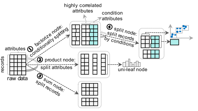
Figure 3. FLAT Structure Construction Process.

 

    Algorithm FLAT-Offline$(A_{\textit{{n}}},C_{\textit{{n}}},T_{\textit{{n}}})$

1: if $C_{\textit{{n}}}=\emptyset$  then

2:    call RDC$(a,b,T_{\textit{{n}}})$ for each pair of attributes $a,b\in A_{\textit{{n}}}$

3:    $H\leftarrow\{a,b|\textsf{RDC}(a,b,T_{\textit{{n}}})\geq\tau_{h}\}$

4:    recursively enlarge $H\leftarrow H\cup\{c|\textsf{RDC}(a,c,T_{\textit{{n}}})\geq\tau_{h},a\in H,c\notin H\}$

5:    if $H\neq\emptyset$ then

6:       $O_{\textit{{n}}}\leftarrow\textsf{factorize}$

7:       call $\textsf{FLAT-Offline}(A_{\textit{{n}}}-H,\emptyset,T_{\textit{{n}}})$ on the left child of node $N$

8:       call $\textsf{FLAT-Offline}(H,A_{\textit{{n}}}-H,T_{\textit{{n}}})$ on the right child of node $N$

9:    else if $|A_{\textit{{n}}}|=1$ then

10:       $O_{\textit{{n}}}\leftarrow\textsf{uni-leaf}$

11:       $\Pr_{\textit{{t}}_{\textit{{n}}}}(A_{\textit{{n}}})\leftarrow\textsf{Leaf-PDF}(A_{\textit{{n}}},T_{\textit{{n}}})$

12:    else if subsets $A_{1},A_{2},\dots,A_{m}$ are mutually indepedent then

13:       $O_{\textit{{n}}}\leftarrow\textsf{product}$

14:       call $\textsf{FLAT-Offline}(A_{i},\emptyset,T_{\textit{{n}}}[A_{\textit{{n}}}])$ on each child of $N$ for all $1\leq i\leq m$

15:    else

16:       $O_{\textit{{n}}}\leftarrow\textsf{sum}$

17:       $T_{1},T_{2},\dots,T_{n}\leftarrow\textsf{Cluster}(T_{\textit{{n}}},A_{\textit{{n}}})$

18:       $w_{i}\leftarrow{|T_{i}|}/{|T_{\textit{{n}}}|}$ for all $1\leq i\leq n$

19:       call $\textsf{FLAT-Offline}(A_{\textit{{n}}},\emptyset,T_{i})$ with weight $w_{i}$ on each child of $N$ for $1\leq i\leq n$

20: else

21:    $m\leftarrow\max_{a\in\textit{{a}}_{\textit{{n}}},c\in\textit{{c}}_{\textit{{n}}}}\textsf{RDC}(a,c,T_{\textit{{n}}})$

22:    if $m\leq\tau_{l}$ then

23:       $O_{\textit{{n}}}\leftarrow\textsf{multi-leaf}$

24:       $\Pr_{\textit{{t}}_{\textit{{n}}}}(A_{\textit{{n}}})\leftarrow\textsf{Leaf-PDF}(A_{\textit{{n}}},T_{\textit{{n}}})$

25:       keep the range of $N$ in the attribute domain space

26:    else

27:       $O_{\textit{{n}}}\leftarrow\textsf{split}$

28:       $c\leftarrow\arg\max_{a\in\textit{{a}}_{\textit{{n}}},c\in\textit{{c}}_{\textit{{n}}}}\textsf{RDC}(a,c,T_{\textit{{n}}})$

29:       divide $T_{\textit{{n}}}$ into $T_{1},T_{2},\dots,T_{d}$ by the range on attribute $c$

30:       call $\textsf{FLAT-Offline}(A_{\textit{{n}}},C_{\textit{{n}}},T_{i})$ on each child of $N$ for $1\leq i\leq d$

 

3. Modeling conditional PDF (lines 21–30): when $C_{\textit{{n}}}\neq\emptyset$, we try to model the conditional PDF $\Pr_{T_{\textit{{n}}}}(A_{\textit{{n}}}|C_{\textit{{n}}})$. First, we compute pairwise correlations across all attributes in $A_{\textit{{n}}}$ and $C_{\textit{{n}}}$ (line 21). If $A_{\textit{{n}}}$ is independent of $C_{\textit{{n}}}$, $N$ is a multi-leaf node. We model the multivariate PDF $\Pr_{T_{\textit{{n}}}}(A_{\textit{{n}}})$ using the piecewise regression technique (McZgee and Carleton, 1970) and maintain its range in the attribute domain space (lines 23–25).

Otherwise, we further split records in $T_{\textit{{n}}}$ (step ④ in Figure 3). Probability computation requires $T_{\textit{{n}}}$ to be divided into grids in terms of $C_{\textit{{n}}}$. We apply a heuristic $d$-way partition method where $d$ is a hyper-parameter. We choose the attribute $c\in C_{\textit{{n}}}$ that maximizes the pairwise correlations between $A_{\textit{{n}}}$ and $C_{\textit{{n}}}$ (line 28). Intuitively, dividing the space by $c$ would largely break their correlations. We set $N$ to be a split node, evenly divide the range of $c$ on $T_{\textit{{n}}}$ into $d$ parts and get the clusters $T_{1},T_{2},\dots,T_{d}$ (line 29). After that, we call FLAT-Offline to model $\Pr_{T_{i}}(A_{\textit{{n}}}|C_{\textit{{n}}})$ for each $1\leq i\leq d$ (line 30).

Complexity Analysis. Let $n$ be the number of nodes in the resulting FSPN and $s$ be the number of sum nodes. On each inner node, we can sample a set of $r$ records from table $T$ to compute the RDC scores between attributes. The time cost of calling RDC is $O(r\log r)$, so the total time cost is $O(n{|A|}^{2}r\log r)$. On each sum node, we can also use the sampled records to compute the central points of the clusters and then assign each record to the nearest cluster. We denote the maximum iteration time in $k$-means as $t$. The total clustering time cost on all sum nodes is $O(stkr)$. Besides, on each node, we need to scan all records in $T$ to assign them to the children (for inner nodes) or building the PDFs (for leaf nodes). The total scanning time cost is $O(n|T|)$. Therefore, the time complexity of FLAT-Offline is $O(n{|A|}^{2}r\log r+n|T|+stkr)$. As $n$ is often small, it is efficient. By our testing, learning the structure of an FSPN is faster than SPN and DAR to model the same joint PDF.

4.3. Incremental Updates

When the table $T$ changes, we apply an incremental update method FLAT-Update to ensure the underlying FSPN model can fit the new data. To attain high estimation accuracy while saving update cost, we try to preserve the original FSPN structure to the maximum extent while fine-tuning its parameters for better fitting.

Let $\Delta T$ be the new data inserted into (or deleted from) $T$. We could traverse the FSPN in a top-down manner to fit $T+\Delta T$ (or $T-\Delta T$). Specifically, for each factorize node $N$, since the conditional factorization is a lossless decomposition of the joint PDF, we directly propagate $\Delta T$ to its children. For each split node, we propagate each record in $\Delta T$ to the corresponding child according to its splitting condition.

On each original multi-leaf node $L$, we recheck whether the conditional independence still holds after adding (or deleting) some records. If so, we just update the parameters of its multivariate PDF by $\Delta T$. Otherwise, we reset it as a split node and run lines 28–30 of FLAT-Offline to further divide its domain space.

For each sum node, we store the centroids of all clusters in structure construction. We could assign each record in $\Delta T$ to the nearest cluster (or remove each record from its original cluster), propagate it to that child and update the weight of each child accordingly.

For each product node, we also recheck whether the independence between attributes subset still holds after adding (or deleting) some records. If not, we run lines 12–19 of FLAT-Offline to reconstruct the sub-structure of the FSPN. Otherwise, we directly pass $\Delta T$ to its children. On each uni-leaf node, we update its parameters of the univariate PDF by $\Delta T$. Obviously, after updating, the generated FSPN can accurately fit the PDF of $T+\Delta T$ (or $T-\Delta T$).

Due to space limits, we put the pseudocode of FLAT-Update in Appendix B.1 of the technical report (Zhu et al., 2020). It can run in the background of the DBMS. Note that, FLAT-Update does not change the original FSPN model when the data distribution keeps the same. In case of significant change of data or data schema changes, such as inserting or deleting attributes, the FSPN could be rebuilt by calling FLAT-Offline in Section 4.2.

 

    Algorithm FLAT-Multi$(D,Q)$

1: organize all tables in $D$ as a join tree $J$% offline

2: for each edge $(A,B)\in J$ do

3:    if RDC$(a,b)\geq\tau_{l}$ for any attribute $a$ of $A$ and $b$ of $B$ then

4:       $A\leftarrow\{A,B\}$

5: for each node $T$ in $J$ with attributes $A_{\textit{{t}}}$ of $\mathcal{T}$ do

6:    add scattering coefficient columns $S_{\textit{{t}}}$ in $T$

7:    $\mathcal{F}_{\textit{{t}}}\leftarrow\textsf{FLAT-Offline}(A_{\textit{{t}}}\cup S_{\textit{{t}}},\emptyset,\mathcal{T})$

8: let $E=\{T_{1},T_{2},\dots,T_{d}\}$ denote all nodes in touched by $Q$ % online

9: for $i\leftarrow 1$ to $d$ do

10:    compute $p_{i}$ in Eq. (1) by Technique II

11: return  $|\mathcal{E}|\cdot\prod_{i=1}^{d}p_{i}$

 

5. Multi-Table CardEst Method

In this section, we discuss how to extend FLAT algorithm to multi-table join queries. We first describe our approach on a high level, and then elaborate the key techniques in details.

Main Idea. To avoid ambiguity, in the following, we use printed letters, such as $T,D$, to represent a set of tables, and calligraphic letters, such as $\mathcal{T,D}$, to represent the corresponding full outer join table. Given a database $D$, all information of $D$ is contained in $\mathcal{D}$. DAR-based approach (Yang et al., 2021) builds a single large model on $\mathcal{D}$. It is easy to use and applicable to any type of joins between tables in $D$ but suffer from significant limitations. First, no matter how many tables are involved in a query, the entire model has to be used for probability computation, which may be inefficient. Second, the size of $\mathcal{D}$ grow rapidly w.r.t. the number of tables in $D$, so its training cost is high even using samples from $\mathcal{D}$. Third, in case of data update of any table in $D$, the entire model needs to be retrained.

Another approach (Hilprecht et al., 2019) builds a set of small models, where each captures the joint PDF of several tables $D^{\prime}\subseteq D$. The joint PDF of attributes in $\mathcal{D}^{\prime}$ (the full outer join table of $D^{\prime}$) is different from that in $\mathcal{D}$ since each record in $\mathcal{D}^{\prime}$ can appear multiple times in $\mathcal{D}$. Therefore, the local model of $\mathcal{D}^{\prime}$ needs to involve some additional columns to correct such PDF difference. When a query touches tables in multiple models, all local probabilities are corrected and merged together to estimate the final cardinality. This approach is more efficient and flexible, but it only supports the primary-foreign key join. This is not practical as many-to-many joins are very common in query optimization (see Section 6.3 for examples on the benchmark workload).

To overcome their drawbacks, our approach absorbs the key ideas of (Hilprecht et al., 2019) and also builds a set of small local models. However, we extend this method to be more general and applicable. First, we develop a new PDF correction paradigm, inspired by (Hilprecht et al., 2019), to support more types of joins, e.g., inner or outer and many-to-many (See the following Technique I). Second, we specifically optimize the probability computation and correction process based on our FSPN model (See Technique II). Third, we develop incremental model updates method for data changes (See Technique III).

(a) Table $T_{\textit{{a}}}$

$A_{1}$	$A_{2}$
$b$	0
$c$	2
$b$	3
$c$	4

(b) Table $T_{\textit{{b}}}$

$B_{1}$	$B_{2}$	$B_{3}$
1	0.3	$M$
0	0.6	$D$
3	0.4	$D$
2	0.7	$M$
4	0.5	$K$
3	0.2	$K$

(c) Table $T_{\textit{{c}}}$ of node $T_{2}$

$C_{1}$	$C_{2}$	$S_{\textit{{t}}_{2},\{\textit{{t}}_{1},\textit{{t}}_{2}\}}$
$D$	0.2	2
$M$	0.7	2
$D$	0.8	2
$K$	0.9	2

(d) Table $T_{\textit{{a}}}\mathbin{\rule[0.58122pt]{1.98001pt}{0.6pt}\hbox to0.0pt{\hss\rule[3.48746pt]{1.98001pt}{0.6pt}}\mkern-5.5mu\bowtie\mkern-5.5mu\rule[0.58122pt]{1.98001pt}{0.6pt}\hbox to0.0pt{\hss\rule[3.48746pt]{1.98001pt}{0.6pt}}}T_{\textit{{b}}}$ of node $T_{1}$

$A_{1}$	$A_{2}$	$B_{1}$	$B_{2}$	$B_{3}$	$S_{\textit{{a}},\textit{{b}}}$	$S_{\textit{{b}},\textit{{a}}}$	$S_{\textit{{t}}_{1},\{\textit{{t}}_{1},\textit{{t}}_{2}\}}$
null	null	1	0.3	$M$	0	0	1
$b$	0	0	0.6	$D$	1	1	2
$b$	3	3	0.4	$D$	2	1	2
$c$	2	2	0.7	$M$	1	1	1
$c$	4	4	0.5	$K$	1	1	1
$b$	3	3	0.2	$K$	2	1	1

(e) Join Tree $J$ and Query $Q$

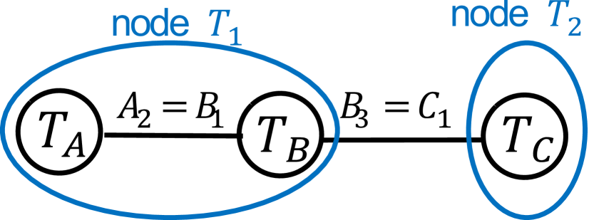
$\boldsymbol{Q}$: select count(*) from $T_{\textit{{b}}}$ full outer join $T_{\textit{{c}}}$ on $T_{\textit{{b}}.\textit{{b}}_{3}}\!=\!T_{\textit{{c}}.\textit{{c}}_{1}}$ where $T_{\textit{{b}}.\textit{{b}}_{2}}\!\!>\!\!0.5$ and $T_{\textit{{c}}.\textit{{c}}_{2}}\!\!<\!\!0.3$

Figure 4. Example databases and join query.

Algorithm Description. We present a high-level description of our approach in the FLAT-Multi algorithm, which takes a database $D$ and a query $Q$ as inputs. The main procedures are as follows:

1. Offline Construction (lines 1–7): We first organize all tables in $D$ as a tree $J$ based on their joins. Initially, each node in $J$ is a table in $D$, and each edge in $J$ is a join between two tables. We do not consider self-join and circular joins in this paper. Based on $J$, we can partition all tables in $D$ into multiple groups such that: tables are highly correlated in the same group but weakly correlated in different groups. Specifically, for each edge $(A,B)$ in $J$, we sample some records from $A\mathbin{\rule[0.6458pt]{2.20001pt}{0.6pt}\hbox to0.0pt{\hss\rule[3.87495pt]{2.20001pt}{0.6pt}}\mkern-5.5mu\bowtie\mkern-5.5mu\rule[0.6458pt]{2.20001pt}{0.6pt}\hbox to0.0pt{\hss\rule[3.87495pt]{2.20001pt}{0.6pt}}}B$, the outer join table, and examine the pairwise attribute correlation values between $A$ and $B$. If some correlation values are higher than a threshold, we learn the model on $A\mathbin{\rule[0.6458pt]{2.20001pt}{0.6pt}\hbox to0.0pt{\hss\rule[3.87495pt]{2.20001pt}{0.6pt}}\mkern-5.5mu\bowtie\mkern-5.5mu\rule[0.6458pt]{2.20001pt}{0.6pt}\hbox to0.0pt{\hss\rule[3.87495pt]{2.20001pt}{0.6pt}}}B$ together, so we merge $\{A,B\}$ to a single node. We repeat this process until no pair of nodes needs to be merged. After that, the probability across different nodes can roughly be assumed as independent on their full outer join table.

After the partition, each node $T$ in $J$ represents a set of one or more single tables. We add some scattering coefficient columns in its outer join table $\mathcal{T}$ for PDF correction. The details are explained in the following Technique I. Then, we construct a FSPN $\mathcal{F}_{\textit{{t}}}$ on $\mathcal{T}$ using FLAT-Offline in Section 4.2. If $\mathcal{T}$ is large, we do not explicitly materialize it. Instead, we draw some samples from $\mathcal{T}$ using the method in (Zhao et al., 2018) and train the FSPN model on them.

Figure 4 depicts a example database with three tables. The join between $T_{\textit{{b}}}$ and $T_{\textit{{c}}}$ is a many-to-many join. $T_{\textit{{a}}}$ and $T_{\textit{{b}}}$ are highly correlated so they are merged together into node $T_{1}$. Then, we build two FSPNs $\mathcal{F}_{\textit{{t}}_{1}}$ and $\mathcal{F}_{\textit{{t}}_{2}}$ on table $T_{\textit{{a}}}\mathbin{\rule[0.6458pt]{2.20001pt}{0.6pt}\hbox to0.0pt{\hss\rule[3.87495pt]{2.20001pt}{0.6pt}}\mkern-5.5mu\bowtie\mkern-5.5mu\rule[0.6458pt]{2.20001pt}{0.6pt}\hbox to0.0pt{\hss\rule[3.87495pt]{2.20001pt}{0.6pt}}}T_{\textit{{b}}}$ and $T_{\textit{{c}}}$, respectively.

2. Online Processing (lines 8–12): Let $E=\{T_{1},T_{2},\dots,T_{d}\}$ denote all nodes in $J$ touched by the query $Q$ and $Q_{i}$ be the sub-query on $T_{i}$. By our assumption, the probability of each $Q_{i}$ is independent on the table $\mathcal{E}=\mathcal{T}_{1}\mathbin{\rule[0.6458pt]{2.20001pt}{0.6pt}\hbox to0.0pt{\hss\rule[3.87495pt]{2.20001pt}{0.6pt}}\mkern-5.5mu\bowtie\mkern-5.5mu\rule[0.6458pt]{2.20001pt}{0.6pt}\hbox to0.0pt{\hss\rule[3.87495pt]{2.20001pt}{0.6pt}}}\mathcal{T}_{2}\mathbin{\rule[0.6458pt]{2.20001pt}{0.6pt}\hbox to0.0pt{\hss\rule[3.87495pt]{2.20001pt}{0.6pt}}\mkern-5.5mu\bowtie\mkern-5.5mu\rule[0.6458pt]{2.20001pt}{0.6pt}\hbox to0.0pt{\hss\rule[3.87495pt]{2.20001pt}{0.6pt}}}\dots\mathbin{\rule[0.6458pt]{2.20001pt}{0.6pt}\hbox to0.0pt{\hss\rule[3.87495pt]{2.20001pt}{0.6pt}}\mkern-5.5mu\bowtie\mkern-5.5mu\rule[0.6458pt]{2.20001pt}{0.6pt}\hbox to0.0pt{\hss\rule[3.87495pt]{2.20001pt}{0.6pt}}}\mathcal{T}_{d}$. We can efficiently correct the probability from the local model $\mathcal{F}_{\textit{{t}}_{i}}$ on $\mathcal{T}_{i}$ to $\mathcal{E}$ by a new paradigm. Finally, we multiply all probabilities to get the final result.

Technique I: Probability Correction Method. We need to correct the probability to account for the effects of joining from two aspects. We elaborate the details with the example query $Q$ in Figure 4(e). $Q$ is divided into two sub-queries: $Q_{1}$ ($T_{\textit{{b}}.\textit{{b}}_{2}}\!>\!0.5$ on node $T_{1}$) and $Q_{2}$ ($T_{\textit{{c}}.\textit{{c}}_{2}}<0.3$ on node $T_{2}$). First, on node $T_{1}$, the FSPN $\mathcal{F}_{\textit{{t}}_{1}}$ is built on table $T_{\textit{{a}}}\mathbin{\rule[0.6458pt]{2.20001pt}{0.6pt}\hbox to0.0pt{\hss\rule[3.87495pt]{2.20001pt}{0.6pt}}\mkern-5.5mu\bowtie\mkern-5.5mu\rule[0.6458pt]{2.20001pt}{0.6pt}\hbox to0.0pt{\hss\rule[3.87495pt]{2.20001pt}{0.6pt}}}T_{\textit{{b}}}$ instead of table $T_{\textit{{b}}}$ individually. As each record in $T_{\textit{{b}}}$ can occur multiple times in $T_{\textit{{a}}}\mathbin{\rule[0.6458pt]{2.20001pt}{0.6pt}\hbox to0.0pt{\hss\rule[3.87495pt]{2.20001pt}{0.6pt}}\mkern-5.5mu\bowtie\mkern-5.5mu\rule[0.6458pt]{2.20001pt}{0.6pt}\hbox to0.0pt{\hss\rule[3.87495pt]{2.20001pt}{0.6pt}}}T_{\textit{{b}}}$, the probability obtained by $\mathcal{F}_{\textit{{t}}_{1}}$ needs to be down-scaled to remove the effects of $T_{\textit{{a}}}$. Second, the probability obtained on node $T_{2}$ is defined on table $T_{\textit{{c}}}$ individually but not on $T_{\textit{{b}}}\mathbin{\rule[0.6458pt]{2.20001pt}{0.6pt}\hbox to0.0pt{\hss\rule[3.87495pt]{2.20001pt}{0.6pt}}\mkern-5.5mu\bowtie\mkern-5.5mu\rule[0.6458pt]{2.20001pt}{0.6pt}\hbox to0.0pt{\hss\rule[3.87495pt]{2.20001pt}{0.6pt}}}T_{\textit{{c}}}$. Therefore, the probability of $Q_{2}$ (and also $Q_{1}$) needs to be up-scaled to add the effects of joining.

The above corrections are achieved by adding extra columns in table $\mathcal{T}_{i}$ of each node $T_{i}$. These columns track the number of times that a record in a single table $A$ appears in $\mathcal{T}_{i}$, i.e., the scattering effect. Previous works (Hilprecht et al., 2019; Yang et al., 2021) add columns to process the scattering effects of each join in only one side. However, our solution considers the scattering effects on two sides of each join. It is more practical by supporting more join types in one framework, and more general by processing down-scale and up-scale effects at the same time.

For each pair of joined tables $(A,B)$ in a node $T_{i}$, we add two additional attributes $S_{\textit{{a}},\textit{{b}}}$ and $S_{\textit{{b}},\textit{{a}}}$ in $\mathcal{T}_{i}$. $S_{\textit{{a}},\textit{{b}}}$ indicates how many records in $B$ can join with this record in $A$ and vice versa. We call such $S_{\textit{{a}},\textit{{b}}}$ scattering coefficient. In Figure 4(d), we add two columns $S_{\textit{{a}},\textit{{b}}}$ and $S_{\textit{{b}},\textit{{a}}}$ in the table $T_{\textit{{a}}}\mathbin{\rule[0.6458pt]{2.20001pt}{0.6pt}\hbox to0.0pt{\hss\rule[3.87495pt]{2.20001pt}{0.6pt}}\mkern-5.5mu\bowtie\mkern-5.5mu\rule[0.6458pt]{2.20001pt}{0.6pt}\hbox to0.0pt{\hss\rule[3.87495pt]{2.20001pt}{0.6pt}}}T_{\textit{{b}}}$ of $T_{1}$. These columns are be used to down-scale the effects of untouched tables inside each node.

Similarly, for up-scale correction, we can regard node $T_{i}$ as the root of the join tree $J$. For each distinct sub-tree of $J$ rooted at $T_{i}$ containing nodes $E^{\prime}=\{T_{1}^{\prime},T_{2}^{\prime},\dots,T_{d}^{\prime}\}$, we add a column $S_{\textit{{t}}_{i},E^{\prime}}$ in table $\mathcal{T}_{i}$ indicating the scattering coefficient of each record in $\mathcal{T}_{i}$ to the outer join table $\mathcal{E}^{\prime}=\mathcal{T}^{\prime}_{1}\mathbin{\rule[0.6458pt]{2.20001pt}{0.6pt}\hbox to0.0pt{\hss\rule[3.87495pt]{2.20001pt}{0.6pt}}\mkern-5.5mu\bowtie\mkern-5.5mu\rule[0.6458pt]{2.20001pt}{0.6pt}\hbox to0.0pt{\hss\rule[3.87495pt]{2.20001pt}{0.6pt}}}\mathcal{T}^{\prime}_{2}\mathbin{\rule[0.6458pt]{2.20001pt}{0.6pt}\hbox to0.0pt{\hss\rule[3.87495pt]{2.20001pt}{0.6pt}}\mkern-5.5mu\bowtie\mkern-5.5mu\rule[0.6458pt]{2.20001pt}{0.6pt}\hbox to0.0pt{\hss\rule[3.87495pt]{2.20001pt}{0.6pt}}}\dots\mathbin{\rule[0.6458pt]{2.20001pt}{0.6pt}\hbox to0.0pt{\hss\rule[3.87495pt]{2.20001pt}{0.6pt}}\mkern-5.5mu\bowtie\mkern-5.5mu\rule[0.6458pt]{2.20001pt}{0.6pt}\hbox to0.0pt{\hss\rule[3.87495pt]{2.20001pt}{0.6pt}}}\mathcal{T}^{\prime}_{d}$. For the node $T_{2}$ in Figure 4(c), we add the column $S_{\textit{{t}}_{2},\{\textit{{t}}_{1},\textit{{t}}_{2}\}}$ indicating the scattering coefficient of each record in $T_{\textit{{c}}}$ when joining with $T_{\textit{{a}}}\mathbin{\rule[0.6458pt]{2.20001pt}{0.6pt}\hbox to0.0pt{\hss\rule[3.87495pt]{2.20001pt}{0.6pt}}\mkern-5.5mu\bowtie\mkern-5.5mu\rule[0.6458pt]{2.20001pt}{0.6pt}\hbox to0.0pt{\hss\rule[3.87495pt]{2.20001pt}{0.6pt}}}T_{\textit{{b}}}$. The method to compute the values of these scattering coefficient columns has been proposed in (Zhao et al., 2018). Briefly speaking, we can obtain the values of $S_{\textit{{t}}_{i},E^{\prime}}$ by recursively aggregating over all sub-trees rooted at $T_{i}$’s children. Using dynamic programming, the time cost of computing scatter coefficient values over all nodes is linear w.r.t. table size.

As all tables form a join tree, the number of added scattering columns in each node is linear w.r.t. its number of tables. In each node $T_{i}$, all scattering coefficient columns are learned together with other attributes when constructing the FSPN $\mathcal{F}_{\textit{{t}}_{i}}$.

We can estimate the cardinality by the following lemma. We put the detailed correctness proof in Appendix C of the technical report (Zhu et al., 2020). In a high order, for each record with down-scale value $s$ and up-scale value $e$, we correct its probability satisfying $Q_{i}$ by a factor of $e/s$. We set $e$ or $s$ to $1$ if it is $0$ since records with zero scattering coefficient also occur once in the full outer join table.

Lemma 2 Given a query $Q$, let $E=\{T_{1},T_{2},\dots,T_{d}\}$ denote all nodes in $J$ touched by $Q$. On each node $T_{i}$, let $S=\{S_{\textit{{a}}_{1},\textit{{b}}_{1}},S_{\textit{{a}}_{2},\textit{{b}}_{2}},\dots,\break S_{\textit{{a}}_{n},\textit{{b}}_{n}}\}$, where each $(A_{j},B_{j})$ is a distinct join such that $B_{j}$ is not in $Q$. Let $s=(s_{1},s_{2},\dots,s_{n})$ where $S_{\textit{{a}}_{j},\textit{{b}}_{j}}=s_{j}\in\mathbb{N}$ for all $1\leq i\leq n$ denote an assignment to $S$ and $\text{dlm}(s)=\prod_{j=1}^{n}\max\{s_{j},1\}$. Let

(1) $$p_{i}\!=\frac{|\mathcal{T}_{i}|}{|\mathcal{E}|}\!\cdot\!\sum\limits_{s,e}\left(\Pr\nolimits_{\mathcal{T}_{i}}(Q_{i}\wedge S\!=\!s\wedge S_{\textit{{t}}_{i},\textit{{e}}}\!=\!e)\cdot\frac{\max\{e,1\}}{\text{dlm}(s)}\right).$$

Then, the cardinality of $Q$ is $|\mathcal{E}|\cdot\prod_{i=1}^{d}p_{i}$.

Consider again query $Q$ in Figure 4(e). For the sub-query $Q_{1}$ on node $T_{1}$, we need to down-scale by $S_{\textit{{b}},\textit{{a}}}$ and up-scale by $S_{\textit{{t}}_{1},\{\textit{{t}}_{1},\textit{{t}}_{2}\}}$. By Eq. (1), we have $p_{1}=(1*2+1+1)/8=1/2$. Similarly, we have $p_{2}=1/4$ for sub-query $Q_{2}$, so the final cardinality of $Q$ is $8*(1/8)=1$.

As a remark, if two tables $A$ and $B$ are inner joined in $Q$, we can add the constraint $S_{\textit{{a}},\textit{{b}}}\!>\!0$ and $S_{\textit{{b}},\textit{{a}}}\!>\!0$ (or $S_{\textit{{a}},\textit{{e}}}\!>\!0$ and $S_{\textit{{b}},\textit{{e}}}\!>\!0$ if $A$ and $B$ in different nodes) in Eq. (1) to remove all records in $A$ or $B$ that have no matches. Similarly, we only add $S_{\textit{{b}},\textit{{a}}}>0$ or $S_{\textit{{a}},\textit{{b}}}>0$ to $Q$ for left and right join, respectively.

Technique II: Fast Probability Computation: Notice that, the value $p_{i}$ in Eq. (1) involves summing over the probabilities of each assignment to the down-scale value $s$ and up-scale value $e$. If we directly obtain all these probabilities, the time cost is very high. Instead, we present an optimized method to compute $p_{i}$, which only requires a single traversal on the underlying FSPN model.

Specifically, on any node $T$ in the join tree, let $S_{\textit{{t}}}$ and $A_{\textit{{t}}}$ denote the scattering coefficient and attribute columns in $\mathcal{T}$, respectively. When constructing the FSPN $\mathcal{F}_{\textit{{t}}}$, we first use a factorize root node to split the joint PDF $\Pr_{\mathcal{T}}(S_{\textit{{t}}},A_{\textit{{t}}})$ into $\Pr_{\mathcal{T}}(A_{\textit{{t}}})$ on the left child $LC$ and $\Pr_{\mathcal{T}}(S_{\textit{{t}}}|A_{\textit{{t}}})$ on the right child $RC$. Each leaf node $L$ of $RC$ models a PDF of $S_{\textit{{t}}}$. By FSPN’s semantic, the probabilities of any query $Q$ on $A_{\textit{{t}}}$ and $S_{\textit{{t}}}$ are independent on each $L$. Then, we have

(2) $$\small\begin{split}\Pr^{\prime}\nolimits_{\mathcal{T}}(Q)\!&=\!\!\sum_{\textit{{l}}}\left(\Pr\nolimits_{\textit{{l}}}(A_{\textit{{t}}})\!\cdot\!\sum_{s,e}\left(\Pr\nolimits_{\textit{{l}}}(S=s\wedge S_{\textit{{t}},\textit{{e}}}=e)\cdot\frac{\max\{e,1\}}{\text{dlm}(s)}\right)\right)\\ &=\!\!\sum_{\textit{{l}}}\left(\Pr\nolimits_{\textit{{l}}}(A_{\textit{{t}}})\!\cdot\mathbb{E}\left[\frac{\max\{e,1\}}{\text{dlm}(s)}\right]\!\right).\end{split}$$

For the left part, the probability $\Pr_{\textit{{l}}}(A_{\textit{{t}}})$ could be computed with the FSPN rooted at node $LC$ using the method in Section 4.1. For the right part, it is a fixed expected value of $\max\{e,1\}/\text{dlm}(s)$ of $S_{\textit{{t}}}$. Therefore, we can pre-compute the expected value for each possible $S,S_{\textit{{t}},\textit{{e}}}\subseteq S_{\textit{{t}}}$ on each leaf $L$. After that, each $p_{i}$ in Eq. (1) could be obtained by traversing the FSPN $\mathcal{F}_{\textit{{t}}_{i}}$ only once. By our empirical analysis in Section 4.1, the CardEst time cost for multi-table queries is also near linear w.r.t. the number of nodes in FSPNs.

Technique III: Incremental Updates. Next, we introduce how to update the underlying FSPN models in multi-table cases. We put the pseudocode of our algorithm FLAT-Update-Multi in Appendix B.2 (Zhu et al., 2020) and describe the procedures as follows.

First, we consider the case of inserting some records $\Delta C$ in a table $C$ of the node $T$. It affects $\mathcal{T}$ in three aspects: 1) each record in $\Delta C$ can join with other tables in $T$. We use $\Delta\mathcal{T_{+}}$ to denote all new records inserted into $\mathcal{T}$; 2) each record in $\mathcal{T}$, which does not find a match in table $C$ (null) but can join with the new records in $\Delta C$, needs to be removed. We denote them as $\Delta\mathcal{T_{-}}$; and 3) the scattering coefficient of each record in $\mathcal{T}$, which can join with new records in $\Delta C$, needs to be enlarged. We denote these records as $\Delta\mathcal{T_{*}}$. We can directly join $\Delta C$ with $\mathcal{T}$ to identify $\Delta\mathcal{T_{+}}$, $\Delta\mathcal{T_{-}}$ and $\Delta\mathcal{T_{*}}$ accordingly.

Next, we describe how to incrementally update the FSPN $\mathcal{F}_{\textit{{t}}}$ built by Technique II. Recall that the root node $N$ of $\mathcal{F}_{\textit{{t}}}$ is a factorize node separating attributes and scattering coefficient columns, which enables fast incremental update. The left child $LC$ of $N$ models $\Pr_{\mathcal{T}}(A_{\textit{{t}}})$ on all attribute columns. We could update it to fit the data $\mathcal{T}+\Delta\mathcal{T_{+}}-\Delta\mathcal{T_{-}}$ by directly calling the FLAT-Update method in Section 4.3. The right child $RC$ of $N$ models $\Pr_{\mathcal{T}}(S_{\textit{{t}}}|A_{\textit{{t}}})$ on all scattering coefficients columns. Each multi-leaf $L$ of $RC$ only stores some expected values of $S_{\textit{{t}}}$ defined by Eq. (2). We can pre-build a hash table on the probability of each assignment $s$ of $S_{\textit{{t}}}$. Then, based on the changes of scattering columns in $\Delta\mathcal{T_{+}}$, $\Delta\mathcal{T_{-}}$ and $\Delta\mathcal{T_{*}}$, we can incrementally update all expected values.

Finally, as $\mathcal{T}$ changes, we need to propagate the effects to other nodes $T^{\prime}$ to update all scattering columns $S_{\textit{{t}}^{\prime},\textit{{e}}}$. For efficiency, it can run in the background asynchronously. Specifically, after each time interval such as one day, we scan all tables and recompute the scattering coefficients using the method in (Zhao et al., 2018). Then we incrementally update the expected values stored in FSPN $\mathcal{F}_{\textit{{t}}^{\prime}}$.

For the case of deleting some records $\Delta C$ in a table $C$ of the node $T$, the updating could be done in a very similar way. At this time, we obtain $\Delta\mathcal{T_{-}}$ containing all removed tuples joining with $\Delta C$ previously, $\Delta\mathcal{T_{+}}$ containing all added tuples having no matches in table $C$ and $\Delta\mathcal{T_{*}}$ containing all original records whose scattering coefficients are reduced. Then we update the FSPN $\mathcal{F}_{\textit{{t}}}$ and $\mathcal{F}_{\textit{{t}}^{\prime}}$ of other nodes $T^{\prime}$ in the same way as the insertion case. Notice that, the data insertion and deletion can also be done simultaneously as long as we maintain the proper set of records $\Delta\mathcal{T_{+}}$, $\Delta\mathcal{T_{-}}$ and $\Delta\mathcal{T_{*}}$. In the complex case of creating new tables or deleting existing tables in the database, the model could be retrained offline.

6. Evaluation Results

We have conducted extensive experiments to demonstrate the superiority of our proposed FLAT algorithm. We first introduce the experimental settings, and then report the evaluation results of CardEst algorithms on the single table and multi-table cases in Section 6.1 and 6.2, respectively. Section 6.3 reports the effects of updates. Finally, in Section 6.4, we integrate FLAT into the query optimizer of Postgres (Documentation 12, 2020) and evaluate the end-to-end query optimization performance.

Baselines. We compare FLAT with a variety of representative CardEst algorithms, including:
1) Histogram: the simplest 1-D histogram based CardEst method widely used in DBMS such as SQL Server (Lopes et al., 2019) and Postgres (Documentation 12, 2020).
2) Naru: a DAR based algorithm proposed in (Yang et al., 2019). We adopt the authors’ source code from (Yang and Wu, 2019) with the var-skip speeding up technique (Liang et al., 2020). It utilizes a DNN with 5 hidden layers (512, 256, 512, 128, 1024 neuron units) to approximate the PDFs. The sampling size is set to $2,000$ as the authors’ default. We do not compare with the similar method in (Hasan et al., 2019), since their performance is close.
3) NeuroCard (Yang et al., 2021): an extension of Naru onto the multi-table case. We also adopt the authors’ source code from (Luan et al., 2020) and set the sampling size to $8,000$ as the authors’ default.
4) BN: a Bayesian network based algorithm. We use the Chow-Liu Tree (Chow and Liu, 1968; Halford et al., 2019) based implementation to build the BN structure, since its performance is better than others (Getoor et al., 2001; Tzoumas et al., 2011).
5) DeepDB: a SPN based algorithm proposed in (Hilprecht et al., 2019). We adopt the authors’ source code from (Hilprecht, 2019) and apply the same hyper-parameters, which set the RDC independence threshold to $0.3$ and split each node with at least $1\%$ of the input data.
6) SPN-Multi: a simple extension of SPN with multivariate leaf nodes. It maintains a multi-leaf node if the data volume is below $1\%$ and attributes are still not independent.
7) MaxDiff: a representative M-D histogram based method (Poosala and Ioannidis, 1997). We use the implementation provided in the source code repository of  (Yang and Wu, 2019). We do not compare with the improved methods DBHist (Deshpande et al., 2001), GenHist (Gunopulos et al., 2000) and VIHist (Wang and Sevcik, 2003) are they are not open-sourced.
8) Sample: the method uniformly samples a number of records to estimate the cardinality. We set the sampling size to $1\%$ of the dataset. It is used in DBMS such as MySQL (Reference Manual, 2020) and MariaDB (Server Documentation, 2020). We do not compare with other method such as IBJS (Leis et al., 2017) since their performance has been verified to be less competitive (Yang and Wu, 2019; Yang et al., 2021; Hilprecht et al., 2019).
9) KDE: kernel density estimator based method for CardEst. We have implemented it using the scikit-learn module (Liu, 2020).
10) MSCN: a state-of-the-art query-driven CardEst algorithm described in (Kipf et al., 2019). For each dataset, we train it with $10^{5}$ queries generated in the same way as the workload.

Regarding FLAT hyper-parameters as described in Section 4.2, we set the RDC threshold $\tau_{l}=0.3$ and $\tau_{h}=0.7$ for filtering independent and highly correlated attributes, respectively, and set $d=2$ for $d$-way partition of records. Similar to DeepDB, we also do not split a node when it contains less than $1\%$ of the input data. The sensitivity analysis of hyper-parameters are put in Appendix D (Zhu et al., 2020).

Evaluation Metrics. Based on our discussion in Section 1, we concentrate on examining three key metrics: estimation accuracy, time efficiency and storage overhead. For estimation accuracy, we adopt the widely used q-error metric (Yang et al., 2019; Hilprecht et al., 2019; Hasan et al., 2019; Kipf et al., 2019; Leis et al., 2018, 2015) defined as the larger value of$\textsf{Card}(T,Q)/\widehat{\textsf{Card}}(T,Q)$ and $\widehat{\textsf{Card}}(T,Q)/\textsf{Card}(T,Q)$, so its optimal value $1$. We report the whole q-error distribution ($50\%$, $90\%$, $95\%$, $99\%$ and $100\%$ quantile) of each workload. For time efficiency, we report the estimation latency and model training time. For storage overhead, we report the model size.

Environment. All above algorithms have been implemented in Python. All experiments are performed on a CentOS Server with an Intel Xeon Platinum 8163 2.50GHz CPU having 64 cores, 128GB DDR4 main memory and 1TB SSD.

6.1. Single Table Evaluation Results

We use two single table datasets: 1) GAS is real-world gas sensing data obtained from the UCI dataset (Repository, 2020) and contains 3,843,159 records. We extract the most informative 8 columns (Time, Humidity, Temperature, Flow_rate, Heater_voltage, R1, R5 and R7); and 2) DMV (New York, 2020) is a real-world vehicle registration information dataset and contains 11,591,877 tuples. We use the same 11 columns as (Yang and Wu, 2019).

For each dataset, we generate a workload containing $10^{5}$ randomly generated queries. For each query, we use a probability of $0.5$ to decide whether an attribute should be contained. As stated in Section 2, the domain of each attribute $A$ is mapped into an interval, so we uniformly sample two values $l$ and $h$ from the interval such that $l\leq h$ and set $A\in[l,h]$.

Estimation Accuracy. Table 1 reports the q-error distribution for different CardEst algorithms. As main take-away, their accuracy can be ranked as $\textsf{FLAT }\!\approx\!\textsf{Naru}\!\!\approx\!\textsf{SPN-Multi}\!>\!\textsf{BN}\!>\!\textsf{DeepDB}\!>>\!\textsf{Sample}/\textsf{MSCN}>>\textsf{KDE}>>\textsf{MaxDiff}/\textsf{Histogram}$. The details are as follows:

1) Overall, FLAT ’s estimation accuracy is very high. On both datasets, the median q-error (1.001 and 1.002) is very close to $1$, the optimal value. On GAS, FLAT attains the highest accuracy. The accuracy of Naru and SPN-Multi is comparable to FLAT, which is marginally better than FLAT on DMV. The high accuracy of Naru and stems from its AR based decomposition and the large DNN representing the PDFs. SPN-Multi achieves high accuracy as it models the PDFs of attributes without independence assumption.

2) The accuracy BN and DeepDB is worse than FLAT. At the $95\%$ quantile, FLAT outperforms BN by $3.6\times$ and DeepDB by $71\times$ on GAS. The error of BN mainly arises from its approximate structure construction. DeepDB appears to fail at splitting highly correlated attributes. Thus, it causes relatively large estimation errors for queries involving these attributes.

3) The accuracy of MSCN and Sample appears unstable. FLAT outperforms MSCN by $109\times$ and $1.8\times$ on GAS and DMV, respectively. As MSCN is query-driven, its accuracy relies on if the workload is “similar” to the training samples. Whereas, FLAT outperforms Sample by $4.5\times$ and $56\times$ on GAS and DMV, respectively as the sampling space of DMV is much larger than GAS.

4) FLAT largely outperforms Histogram, MaxDiff and KDE since Histogram and MaxDiff makes coarse-grained independence assumption and KDE may not well characterize high-dimensional data by tuning a good bandwidth for kernel functions (Kiefer et al., 2017).

Table 1. Performance of CardEst algorithms on single table.

								Training
Dataset	Algorithm	50%	90%	95%	99%	Max	Size (KB)	Time (Min)
GAS	Histogram	2.732	53.60	163.0	$2\cdot 10^{6}$	$3\cdot 10^{7}$	34	1.3
	Naru	1.007	1.145	1.340	2.960	16.50	6, 365	216
	BN	1.011	1.208	1.550	4.780	36.80	108	8.2
	DeepDB	1.039	1.765	2.230	95.12	619.2	218	54
	SPN-Multi	1.005	1.169	1.289	1.461	3.702	31,253	62
	MaxDiff	2.211	86.7	196.0	$3\cdot 10^{4}$	$8\cdot 10^{5}$	$3\cdot 10^{5}$	310
	Sample	1.046	1.625	2.064	6.017	3, 410	-	-
	KDE	3.307	5.469	6.742	471.0	$2\cdot 10^{4}$	-	27
	MSCN	2.610	68.47	129.0	$1\cdot 10^{5}$	$7\cdot 10^{5}$	2, 663	662
	FLAT (Ours)	1.001	1.127	1.183	1.325	3.178	198	19
DMV	Histogram	1.184	2.541	41.72	710.0	$2\cdot 10^{5}$	24	1.6
	Naru	1.006	1.184	1.368	6.907	49.03	7, 564	146
	BN	1.003	1.264	1.818	9.800	176.0	59	5.4
	DeepDB	1.005	1.574	2.604	27.90	534.0	247	48
	SPN-Multi	1.004	1.163	1.347	7.225	58.37	53,267	53
	MaxDiff	1.802	6.304	28.81	4, 320	$3\cdot 10^{4}$	$7\cdot 10^{5}$	249
	Sample	1.122	1.619	9.010	551.0	7, 077	-	-
	KDE	3.493	15.07	104.0	589.0	$5\cdot 10^{4}$	-	48
	MSCN	1.215	2.612	4.420	17.90	1, 192	2, 566	744
	FLAT (Ours)	1.002	1.255	1.795	9.805	76.50	53	2.4

Estimation Latency. Figure 5 reports the average latency of all CardEst methods. Since only MSCN and Naru provide the implementation optimized for GPUs, we compare all CardEst methods on CPUs for fairness. We provide the comparison results on GPUs in Appendix E.1 (Zhu et al., 2020). In summary, their speed on CPUs can be ranked as $\textsf{Histogram}\approx\textsf{FLAT }>\textsf{MSCN}>\textsf{SPN-Multi}/\textsf{DeepDB}>\textsf{KDE}/\textsf{Sample}>\!>\text{Others}$. The details are as follows:

1) Histogram runs the fastest, it requires around $0.1ms$ for each query. FLAT is close with a latency around $0.2ms$ and $0.5ms$ on DMV and GAS, respectively. Both are much faster than all other methods. This can be credited to the FSPN model used in FLAT being both compact and easy to traverse for probability computation. MSCN is also fast since it only requires a forward pass over DNNs.

2) DeepDB, SPN-Multi, KDE and Sample need up to $10ms$ for each query. FLAT is $1$–$2$ orders of magnitude faster than them because the FSPN model used in our FLAT is more compact than the SPN model in DeepDB and SPN-Multi. In addition, KDE and Sample need to examine large amount of samples, thus less efficient.

3) MaxDiff, BN and Naru need $10$–$100ms$ for each query. FLAT is $2$–$3$ orders of magnitude faster than them, e.g., $213\times$ and $599\times$ faster than Naru on GAS and DMV, respectively. The time cost of MaxDiff is spent on decompressing the joint PDF. The inference on BN is NP-hard and hence inefficient. Naru requires repeated sampling for range querie so it is computationally demanding.

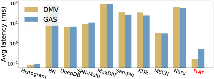
Figure 5. Estimation latency of CardEst algorithms.

Model Training Time. As shown in the last column in Table 1, FLAT is very efficient in training. Specifically, on DMV, FLAT is $61\times$ and $20\times$ faster than Naru and DeepDB in training. This is due to the structure of FSPN is much smaller than SPN, and our training process does not require iterative gradient updates as required for SGD-based training of DNNs (Bottou, 2012).

Storage Overhead. Storage costs are given in Table 1. The storage cost of Histogram and BN is proportional to the attribute number so they require the smallest storage. FLAT is also very small requiring about $2\times$ of Histogram. DeepDB requires more storage space than FLAT since the learned SPN has more nodes. They consume $10$–$100$KB of storage. MSCN and Naru consume several MB since they store large DNN models. SPN-Multi requires tens of MB as it needs to maintain the multi-leaf nodes on not highly correlated attributes, as we discussed in Section 3. The storage cost of MaxDiff is the highest since it stores the compressed joint PDF.

Model Node Number. To give more details, we also compare the number of nodes (or neurons) in DeepDB, SPN-Multi and Naru. The 5-layer DNN in Naru is fully connected and contains $2,432$ neurons. The SPN used in DeepDB contains $873$ and $823$ nodes on GAS and DMV, respectively. SPN-Multi contains $825$ and $787$ nodes on GAS and DMV, respectively. Whereas, the FSPN in FLAT only uses $210$ and $20$ nodes on GAS and DMV, respectively. FSPN uses $21\times$, $7.4\times$ and $7\times$ less nodes than DNN, SPN and SPN-Multi to model the same joint PDF.

Stability. We also examine FLAT on synthetic datasets. The results in Appendix E.2 show that FLAT is stable to varied correlations and distributions and relatively robust to varied domain size.

6.2. Multi-Table Evaluation Results

We evaluate the CardEst algorithms for the multi-table case on the IMDB benchmark dataset. It has been extensively used in prior work (Leis et al., 2018, 2015; Yang et al., 2021; Hilprecht et al., 2019) for cardinality estimation. We use the provided JOB-light query workload with 70 queries and create another more complex and comprehensive workload JOB-ours with $1,500$ queries.

JOB-light’s schema contains six tables (title, cast_info, movie_info, movie_companies, movie_keyword, movie_info_idx) where all other tables can only join with title. Each JOB-light query involves $3$–$6$ tables with $1$–$4$ filtering predicates on all attributes. JOB-ours uses the same schema as JOB-light but each query is a range query using $4$–$6$ tables and $2$–$7$ filtering predicates. The predicate of each attribute is set in the same way as on single table. Figure 6 illustrates the true cardinality distribution of the two workloads. The scope of cardinality for JOB-ours is wider than JOB-light. Note that, the model of each CardEst method is the same for the two workloads. As the attributes are highly correlated on IMDB, the model size of SPN-Multi exceeds our memory limit, so we can not evaluate it.

Results on JOB-light. Table 2 reports the q-error and storage cost of CardEst methods on the JOB-light workload. We observe that:

1) The accuracy of FLAT is the highest among all algorithms. NeuroCard is only a bit better w.r.t the maximum q-error, which reflects only one query in the workload. At the $95\%$ quantile, FLAT outperforms NeuroCard by $2.6\times$, BN by $33\times$, DeepDB by $1.7\times$ and MSCN by $43\times$. The reasons have been explained in Section 6.1.

2) In terms of storage size, Histogram and BN are still the smallest and MaxDiff is still the largest. FLAT ’s space cost is $3.3$MB, which is $10.8\times$ and $2.1\times$ less than DeepDB and NeuroCard, respectively. In comparison with the single table case, FLAT ’s space cost is relatively large. This is because for the multi-table case, FSPN needs to process more attributes—the scattering coefficients columns and materialize some values for fast probability computation. However, it is still reasonable and affordable for modern DBMS.

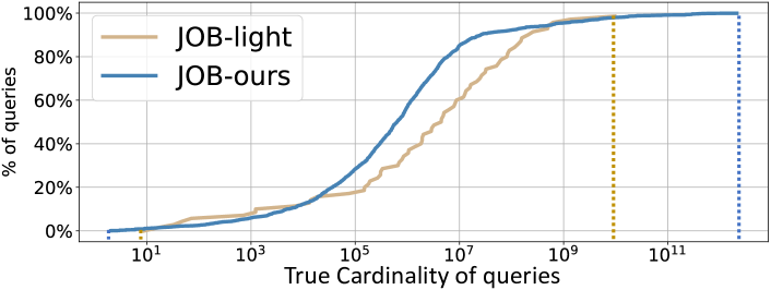
Figure 6. Cardinality distribution of workload on IMDB.

Table 2. Performance of CardEst algorithms on JOB-light.

Algorithm	50%	90%	95%	99%	Max	Size (KB)
Histogram	8.310	1, 386	6, 955	$8\cdot 10^{5}$	$2\cdot 10^{7}$	131
NeuroCard	1.580	4.545	5.910	8.480	8.510	7, 076
BN	2.162	28.00	74.60	241.0	306.0	237
DeepDB	1.250	2.891	3.769	25.10	31.50	$3.7\cdot 10^{4}$
MaxDiff	32.31	5, 682	$5\cdot 10^{4}$	$4\cdot 10^{6}$	$4\cdot 10^{7}$	$4\cdot 10^{5}$
Sample	2.206	65.80	1, 224	$5\cdot 10^{4}$	$1\cdot 10^{6}$	-
KDE	10.56	563.0	4, 326	$4\cdot 10^{5}$	$8\cdot 10^{6}$	-
MSCN	2.750	19.70	97.60	622.0	661.0	3, 421
FLAT (Ours)	1.150	1.819	2.247	7.230	10.86	3, 430

Results on JOB-ours. On this workload, FLAT is also the most accurate CardEst method. As reported in Table 3, we observe that:

1) The performance of FLAT is better than NeuroCard and still much better than others. At the $95\%$ quantile, FLAT outperforms NeuroCard, DeepDB and MSCN by $1.4\times$, $4.3\times$ and $7.8\times$, respectively. The performance of other algorithms drops significantly on this workload. A similar observation is also reported in (Yang et al., 2021). This once again demonstrates the shortcomings of these approaches, especially for complex data and difficult queries.

2) The q-error of FLAT on JOB-ours is relatively larger than that on JOB-light because JOB-ours is a harder workload. As shown in Figure 6, the true cardinality of the tail $5\%$ queries in JOB-ours is often less than $100$. However, the performance of FLAT is still reasonable since the median value is only $1.2$.

We also examine the detailed q-errors of FLAT and other CardEst methods with different number of tables and predicates in queries. Due to space limits, we put the results in Appendix E.3 of the technical report (Zhu et al., 2020). The results show that the accuracy of our FLAT is more stable with number of joins and predicates.

Time Efficiency. Figure 7 exhibits the average estimation latency on the two workload. Obviously, Histogram is still the fastest while MaxDiff is still the slowest. FLAT requires around $5ms$ for each query, which is still much faster than others. It outperforms BN by $5\times$, Sample by $12.4\times$, KDE by $4.8\times$ and DeepDB by $5.2\times$. The training time on the IMDB dataset is given in the last column of Table 3. FLAT is faster than NeuroCard and close to DeepDB.

6.3. Effects of Updates

We examine the performance of our incremental update method. Specifically, for data insertion evaluation, we train the base model on a subset of IMDB data before 2004 ($80\%$ of data) and insert the rest data for updating. For data deletion, we train the base model on all data and delete the data after 1991. We compare the accuracy on the JOB-light workload and the update time cost of our update method with two baselines: he original stale model and the new model retained on the whole data. From Table 4, we observe that:

1) The accuracy of the retrained model is the highest but it requires the highest updating time. The accuracy of the non-updated model is the lowest since the data distribution changes.

2) Our update method makes a good trade-off: its accuracy is close to the retrained model but its time cost is much lower. This shows that our FSPN model can be incrementally updated on its structure and parameters to fit the new data in terms of both insertion and deletion. This is a clear advantage since the entire model does not need to be frequently retrained in presence of new data.

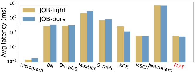
Figure 7. Estimation latency on IMDB.

Table 3. Performance of CardEst algorithms on JOB-ours.

						Training
Algorithm	50%	90	95%	99%	Max	Time (Min)
Histogram	15.71	7480	$4\cdot 10^{4}$	$1\cdot 10^{6}$	$4\cdot 10^{8}$	2.7
NeuroCard	1.538	9.506	81.23	8012	$1\cdot 10^{5}$	173
BN	2.213	25.60	2456	$2\cdot 10^{5}$	$7\cdot 10^{6}$	7.3
DeepDB	1.930	28.30	248.0	$1\cdot 10^{4}$	$1\cdot 10^{5}$	68
MaxDiff	45.50	8007	$2\cdot 10^{5}$	$9\cdot 10^{6}$	$1\cdot 10^{9}$	79
Sample	2.862	116.0	3635	$3\cdot 10^{5}$	$4\cdot 10^{7}$	-
KDE	8.561	1230	$1\cdot 10^{4}$	$9\cdot 10^{5}$	$2\cdot 10^{8}$	15
MSCN	4.961	45.7	447.0	8576	$1\cdot 10^{5}$	1, 744
FLAT (Ours)	1.202	6.495	57.23	1120	$\boldsymbol{1\cdot 10^{4}}$	53

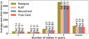
(a) Query Time Excluding CardEst Latency

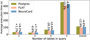
(b) End-to-End Query Time

Figure 8. Comparison of CardEst algorithms integrated into Postgres.

6.4. End-to-End Evaluation on Postgres

To examine the performance of ML-based CardEst algorithms in real-world DBMS, we integrate our FLAT and NeuroCard into the query optimizer of Postgres 9.6.6 to perform an end-to-end test. We do not compare with DeepDB since it can not support many-to-many join. However, for many star-join queries between a primary key and multiple foreign keys in the workload, the sub-queries on joining foreign keys are many-to-many joins. Meanwhile, we add the method which uses the true cardinality of each sub-query during query optimization as the baseline. We report the results of the JOB-light workload on the IMDB benchmark dataset. The results on JOB-ours are similar and put in the Appendix E.4 (Zhu et al., 2020).

We disable parallel computing in Postgres and only allow primary key indexing to minimize the impact of other factors (Van Aken et al., 2017; Leis et al., 2015).We report the total query time excluding the CardEst time cost in Figure 8(a) and the end-to-end query time (including plan compiling and execution) in Figure 8(b). We observe that:

1) Accurate CardEst results can help the query optimizer generate better query plans. Without considering the CardEst latency, both NeuroCard and FLAT improve over Postgres by near $13\%$. Their improvement is very close to the optimal result using true cardinality in query compiling ($14.2\%$). This verifies that the accuracy of FLAT is sufficient to generate high-quality query plans.

2) For the end-to-end query time, the improvement of FLAT is more significant than NeuroCard. Overall, FLAT improves the query time by $12.9\%$ while NeuroCard only improves $4.6\%$. This is due to the CardEst needs to do multiple times in query optimization. The latency of NeuroCard is much longer than FLAT and degrades its end-to-end performance.

3) The improvement of FLAT becomes more significant on queries with more joins. On queries joining $4$ tables, FLAT improves the end-to-end query time by $26.5\%$ because the search space of the query plans grows exponentially w.r.t. the join number. If a query only joins $2$ or $3$ tables, its query plan is almost fixed. When it joins more tables, the inaccurate Postgres results may lead to a sub-optimal query plan while our FLAT providing more accurate CardEst results can find a better plan. This phenomenon has also observed and explained in (Perron et al., 2019).

Table 4. Effects of updates on IMDB.

Update	Method	50%	90%	95%	99%	Max	Time (Min)
Insertion	Non-Updated	1.201	2.297	3.862	18.93	47.14	0
	Retrained	1.150	1.819	2.247	7.230	10.86	53
	Our Method	1.153	1.821	2.480	8.914	13.72	1.2
Deletion	Non-Updated	1.218	2.263	3.905	15.47	56.21	0
	Retrained	1.129	1.763	2.253	6.815	15.3	49
	Our Method	1.134	1.791	2.432	8.285	19.78	1.0

7. Related Work

We briefly review prior work on query-driven CardEst methods and machine learning (ML) applied to problems in databases. The data-driven CardEst methods have already been discussed in Section 2.

Query-Driven CardEst Methods. Initially, prior research has approached query-driven CardEst by utilizing feedback of past queries to correct generated models. Representative work includes correcting and self-tuning histograms with query feedbacks (Bruno et al., 2001; Srivastava et al., 2006; Fuchs et al., 2007; Khachatryan et al., 2015), updating statistical summaries in DBMS (Stillger et al., 2001; Wu et al., 2018), and query-driven kernel-based methods (Heimel et al., 2015; Kiefer et al., 2017). Later on, with the advance of deep learning, focus shifted to learning complex mappings from “featurized” queries to their cardinalities. Different types of models, such as deep networks (Liu et al., 2015), tree-based regression models (Dutt et al., 2019) and multi-set convolutional networks (Kipf et al., 2019), were applied. In general, clear drawbacks of query-driven CardEst methods are as follows: 1) their performance heavily relies on the particular choice of how input queries are transformed into features; 2) they require large amounts of previously executed queries for training; and 3) they only behave well, when future input queries follow the same distribution as the training query samples. Therefore, query-driven CardEst methods are not flexible and generalizable enough.

ML Applied in Databases. Recently, there has been a surge of interest in using ML-based methods in order to enhance the performance of database components, e.g. indexing (Nathan et al., 2020), data layout (Kraska et al., 2018), query execution (Park et al., 2017) and scheduling (Mao et al., 2019). Among them, learned query optimizers are a noteworthy hot-spot. (Marcus et al., 2019) proposed a query plan generation model by learning embeddings for all queries. (Krishnan et al., 2018) applied reinforcement learning to optimize the join order. We are currently trying to integrate FLAT with these two approaches to design an end-to-end solution for query optimization in databases.

Moreover, it is worth mentioning that the proposed FSPN model is a very general unsupervised model, whose scope of application is not limited to CardEst. We are in the process of trying to apply to other scenarios in databases that also require modeling the joint PDF of high-dimensional data, such as approximate group-by query processing (Thirumuruganathan et al., 2020), hashing (Kraska et al., 2018) and multi-dimensional indexing (Nathan et al., 2020).

8. Conclusions

In this paper, we propose FLAT, an unsupervised CardEst method that is simultaneously fast in probability computation, lightweight in storage cost and accurate in estimation quality. It supports queries on both single table and multi-tables. FLAT is built on FSPN, a new graphical model which adaptively models the joint PDF of attributes and combines the advantages of existing CardEst models. Extensive experimental results on benchmarks and the end-to-end evaluation on Postgres have demonstrated the superiority of our proposed methods. In the future work, we believe in that FLAT could serve as a key component in an end-to-end learned query optimizer for DBMS and the general FSPN model can play larger roles in more database-related tasks.

APPENDIX

Appendix A Relations between FSPN and Other Models

We present here the details on how FSPN subsumes SPN, as well as BN models. We assume that all attributes are discrete, i.e., for continuous attributes, we can discretize them by binning, and all (conditional) PDFs are stored in a tabular form.

A.1. Transforming to FSPN

We show the details on how to transform SPN and BN to the equivalent FSPN model.

Transforming from SPN to FSPN. Given a data table $T$ with attributes $A$, if $\Pr_{\textit{{t}}}(A)$ could be represented by an SPN $\mathcal{S}$, we can easily construct an FSPN $\mathcal{F}$ that equally represent $\Pr_{\textit{{t}}}(A)$. Specifically, we disable the factorize operation in FSPN by setting the factorization threshold to $\infty$, and then follow the same steps of $\mathcal{S}$ to construct $\mathcal{F}$. Then, the FSPN $\mathcal{F}$ is exactly the same of $\mathcal{S}$.

Transforming from BN to FSPN. Given a data table $T$ with attributes $A$, if $\Pr_{\textit{{t}}}(A)$ could be represented by a discrete BN $\mathcal{B}$, we can also build an FSPN $\mathcal{F}$ that equally represent $\Pr_{\textit{{t}}}(A)$. Without ambiguity, we also use $\mathcal{B}$ to refer to its DAG structure. We present the procedures in the BN-to-FSPN algorithm. It takes as inputs a discrete BN $\mathcal{B}$ and the root node $N$ of $\mathcal{F}$ and outputs $F_{\textit{{n}}}$ representing the same PDF of $\mathcal{B}$. In general BN-to-FSPN works in a recursive manner by executing the following steps:

① (lines 1–3) If $\mathcal{B}$ contains more than one connected component $\mathcal{B}_{1},\mathcal{B}_{2},\dots,\mathcal{B}_{t}$, the variables in each are mutually independent. Therefore, we set $N$ to be a product node with children $N_{1},N_{2},\dots,N_{t}$ into $\mathcal{F}$, and call BN-to-FSPN on $\mathcal{B}_{i}$ and node $N_{i}$ for each $i$.

② (lines 5–7) If $\mathcal{B}$ contains only one connected component, let $A_{i}$ be a node (variable) in $\mathcal{B}$ that has no out-neighbor. If $A_{i}$ also has no in-neighbor (parent) in $\mathcal{B}$, it maintains the PDF $\Pr_{\textit{{t}}}(A_{i})$. At that time, we set $N$ to be a uni-leaf node representing the univariate distribution $\Pr_{\textit{{t}}}(A_{i})$.

③ (lines 9–16) If the parent set $A_{\text{pa}(i)}$ of $A_{i}$ is not empty, $A_{i}$ has a conditional probability table (CPT) defining $\Pr_{\textit{{t}}}(A_{i}|A_{\text{pa}(i)})=\Pr_{\textit{{t}}}(A_{i}|A\setminus\{A_{i}\})$. At this time, we set $N$ to be a factorize node with the left child representing $\Pr_{\textit{{t}}}(A\setminus\{A_{i}\})$ and right child $N_{\textit{{r}}}$ representing $\Pr_{\textit{{t}}}(A_{i}|A\setminus\{A_{i}\})$. For the right child $N_{\textit{{r}}}$, we set it to be a split node. For each entry $y$ of $A_{\text{pa}(i)}$ in the CPT of $A_{i}$, we add a multi-leaf node $L_{y}$ of $N_{\textit{{r}}}$ containing all data $T_{y}$ in $T$ whose value on $A_{\text{pa}(i)}$ equals $y$. On each leaf $L_{y}$, by the first-order Markov property of BN, $A_{i}$ is conditionally independent of variables $A\setminus\{A_{i}\}\setminus A_{\text{pa}(i)}$ given its parents $A_{\text{pa}(i)}$. Therefore, we can simplify the PDF represented by $L_{y}$ as $\Pr_{\textit{{t}}}(A_{i}|y)=\Pr_{\textit{{t}}_{y}}(A_{i})$. Therefore, $N_{\textit{{r}}}$ characterizes the CPT of $\Pr_{\textit{{t}}}(A_{i}|A_{\text{pa}(i)})=\Pr_{\textit{{t}}}(A_{i}|A\setminus\{A_{i}\})$. Later, we remove the node $A_{i}$ from $\mathcal{B}$ to obtain $\mathcal{B^{\prime}}$, which represents the PDF $\Pr_{\textit{{t}}}(A\setminus\{A_{i}\})$. We call BN-to-FSPN on $\mathcal{B^{\prime}}$ and node $N_{\textit{{l}}}$, the left child of $N$ to further model the PDF.

Finally, we obtain the FSPN $\mathcal{F}$ representing the same PDF of $\mathcal{B}$.

 

    Algorithm BN-to-FSPN$(\mathcal{B},N)$

1:  if $\mathcal{B}$ contains connected components $\mathcal{B}_{1},\mathcal{B}_{2},\dots,\mathcal{B}_{t}$ then

2:     set $N$ to be a product node with children $N_{1},N_{2},\dots,N_{t}$

3:     call BN-to-FSPN$(\mathcal{B}_{i},N_{i})$ for each $i$

4:  else

5:     let $A_{i}$ be a node in $\mathcal{B}$ containing no out-neighbor

6:     if $A_{i}$ has no in-neighbor in $\mathcal{B}$  then

7:        set $N$ to be a uni-leaf node representing $\Pr_{\textit{{t}}}(A_{i})$

8:     else

9:        set $N$ to be a factorize node with left child $N_{\textit{{l}}}$ and right child $N_{\textit{{r}}}$

10:        set $N_{\textit{{r}}}$ to be a split node

11:        for each value $y$ of $A_{\text{pa}(i)}$ in the CPT of $A_{i}$ do

12:           add a multi-leaf node $N_{y}$ as child of $N_{\textit{{r}}}$

13:           let $T_{y}\leftarrow\{t\in T|A_{\text{pa}(i)}\text{ of }t\text{ is }y\}$

14:           let $N_{y}$ represent $\Pr_{\textit{{t}}_{y}}(A_{i})$

15:        remove $A_{i}$ from $\mathcal{B}$ to obtain $\mathcal{B^{\prime}}$

16:        call BN-to-FSPN$(\mathcal{B}^{\prime},N_{\textit{{l}}})$

 

A.2. Proof of Lemma 1

Lemma 1 Given a table $T$ with attributes $A$, if the joint PDF $\Pr_{\textit{{t}}}(A)$ is represented by an SPN $\mathcal{S}$ or a BN $\mathcal{B}$ with space cost $O(M)$, then there exists an FSPN $\mathcal{F}$ that can equivalently model $\Pr_{\textit{{t}}}(A)$ with no more than $O(M)$ space.

Proof.

For the SPN $\mathcal{S}$ and the FLAT $\mathcal{F}$, by Section A.1, their structures are exactly the same. In the simplest case, if $\mathcal{F}$ represents the distribution in the same way as $\mathcal{S}$ on each leaf nodes, their space cost is the same.

For the BN $\mathcal{B}$ and the FLAT $\mathcal{F}$, we analyze their space cost. The storage cost of each node $A_{i}$ in $\mathcal{B}$ is the number of entries in CPT of $\Pr_{\textit{{t}}}(A_{i}|A_{\text{pa}(i)})$. The FSPN $\mathcal{F}$ represents $\Pr_{\textit{{t}}}(A_{i})$ in step ② of algorithm BN-to-FSPN when $A_{\text{pa}(i)}$ is empty and $\Pr_{\textit{{t}}}(A_{i}|y)$ for each value $y$ of $A_{\text{pa}(i)}$ in step ③. In the simplest case, if $\mathcal{F}$ also represents the distribution in a tabular form, the storage cost is the same as $\mathcal{B}$. Therefore, the model size of $\mathcal{F}$ can not be larger than that of $\mathcal{B}$.

Therefore, this lemma holds. ∎

Appendix B Detailed Updating Algorithm

We put the pseudocodes of our incremental updating algorithms.

B.1. FLAT-Update Algorithm

The FLAT-Update algorithm described in Section 4.3 is used for updating FSPN built on single table. It works in a recursive manner and traverse the original FSPN in a top-down manner. FLAT-Update tries to preserve the original FSPN structure to the maximum extent while fine-tuning its parameters for better fitting. The process to each type of nodes have been explained clearly in Section 4.3.

 

    Algorithm FLAT-Update$(\mathcal{F},\Delta T)$

1:  let $N$ be the root node of $\mathcal{F}$

2:  if $N$ is factorize node then

3:     call FLAT-Update$(\mathcal{F}_{\textit{{n}}_{i}},\Delta T)$ for each child $N_{i}$ of $N$

4:  else if $N$ is split node then

5:     for each child $N_{i}$ of $N$ do

6:        let $\Delta T_{i}$ be the set of records in the splitting condition of $N_{i}$

7:        call FLAT-Update$(\mathcal{F}_{\textit{{n}}_{i}},\Delta T_{i})$

8:  else if $N$ is multi-leaf node then

9:     if the conditional indepence still holds on $T_{\textit{{n}}}$ then

10:        update the parameters of the PDF by $\Delta T$

11:     else

12:        reset $N$ to be a split node

13:        call lines 28–30 of FLAT-Offline($A_{\textit{{n}}},C_{\textit{{n}}},T_{\textit{{n}}}$)

14:  else if $N$ is sum node then

15:     for each child $N_{i}$ of $N$ do

16:        let $\Delta T_{i}$ be the set of records assigned to or removed from $N_{i}$

17:        update the weights of $N_{i}$ accordingly

18:        call FLAT-Update$(\mathcal{F}_{\textit{{n}}_{i}},\Delta T_{i})$

19:  else if $N$ is product node then

20:     if the indepence between attributes still holds on $T_{\textit{{n}}}$ then

21:        call FLAT-Update$(\mathcal{F}_{\textit{{n}}_{i}},\Delta T)$ for each child $N_{i}$ of $N$

22:     else

23:        call lines 12–19 of FLAT-Offline($A_{\textit{{n}}},C_{\textit{{n}}},T_{\textit{{n}}}$)

24:  else if $N$ is uni-leaf node then

25:     update the parameters of the PDF by $\Delta T$

 

B.2. FLAT-Update-Multi Algorithm

The FLAT-Update-Multi algorithm described in Technique III of Section 5 is used to update the FSPN models built on multi-tables. We first identify the impact of updating $\Delta C$ onto $\mathcal{T}$, and then update the FSPN modeling attribute columns and scattering coefficients columns, respectively. The details are clearly presented in Section 5.

 

    Algorithm FLAT-Update-Multi$(\mathcal{F}_{\textit{{t}}},\Delta C)$

1:  if $\Delta C$ is inserted into table $C$ then

2:     obtain $\Delta\mathcal{T_{+}}$ with all new records joining with $\Delta C$

3:     obtain $\Delta\mathcal{T_{-}}$ with all records with null attributes of table $C$ but can join with $\Delta C$

4:     obtain $\Delta\mathcal{T_{*}}$ with all original records can join with $\Delta C$

5:  else

6:     obtain $\Delta\mathcal{T_{+}}$ with all new records joining with null attributes of table $C$

7:     obtain $\Delta\mathcal{T_{-}}$ with all removed tuples joining with $\Delta C$

8:     obtain $\Delta\mathcal{T_{*}}$ with all original records can join with $\Delta C$

9:  let $N$ be the root node of $\mathcal{F}$ with left child $LC$ and right child $RC$

10:  call FLAT-Update$(\mathcal{F}_{\textit{{l}}\textit{{c}}},\Delta\mathcal{T_{+}})$

11:  call FLAT-Update$(\mathcal{F}_{\textit{{l}}\textit{{c}}},\Delta\mathcal{T_{-}})$

12:  for each multi-leaf node $L$ of $RC$ do

13:     incrementally update all expected values based on the scattering columns in $\Delta\mathcal{T_{+}}$, $\Delta\mathcal{T_{-}}$ and $\Delta\mathcal{T_{*}}$

14:  if reaches the periodical updating time then

15:     recompute all scattering columns $S_{\textit{{t}},\textit{{e}}}$ for all nodes $T$

16:     if $S_{\textit{{t}},\textit{{e}}}$ changes then

17:        incrementally update all expected values in all multi-leaf nodes

 

Appendix C Proof of Lemma 2

Lemma 2 Given a query $Q$, let $E=\{T_{1},T_{2},\dots,T_{d}\}$ denote all nodes in $J$ touched by $Q$. On each node $T_{i}$, let $S=\{S_{\textit{{a}}_{1},\textit{{b}}_{1}},S_{\textit{{a}}_{2},\textit{{b}}_{2}},\dots,\break S_{\textit{{a}}_{n},\textit{{b}}_{n}}\}$, where each $(A_{j},B_{j})$ is a distinct join such that $B_{j}$ is not in $Q$. Let $s=(s_{1},s_{2},\dots,s_{n})$ where $S_{\textit{{a}}_{j},\textit{{b}}_{j}}=s_{j}\in\mathbb{N}$ for all $1\leq i\leq n$ denote an assignment to $S$ and $\text{dlm}(s)=\prod_{j=1}^{n}\max\{s_{j},1\}$. Let

(1) $$\small p_{i}\!=\frac{|\mathcal{T}_{i}|}{|\mathcal{E}|}\!\cdot\!\sum\limits_{s,e}\left(\Pr\nolimits_{\mathcal{T}_{i}}(Q_{i}\wedge S\!=\!s\wedge S_{\textit{{t}}_{i},\textit{{e}}}\!=\!e)\cdot\frac{\max\{e,1\}}{\text{dlm}(s)}\right).$$

Then, the cardinality of $Q$ is $|\mathcal{E}|\cdot\prod_{i=1}^{d}p_{i}$.

Proof.

Given the query $Q$, let $Z$ denote all the tables touched by $Q$ and $Z_{i}$ be the tables touched by $Q$ in the node $T_{i}$. Obviously, we can obtain the cardinality of $Q$ on table $\mathcal{Z}$ as $\textsf{Card}(\mathcal{Z},Q)=\Pr_{\mathcal{Z}}(Q)\cdot|\mathcal{Z}|$.

First, we have $Z\subseteq T=\cup_{i=1}^{d}T_{i}$. Let $\mathcal{E}=\mathcal{T}_{1}\mathbin{\rule[0.6458pt]{2.20001pt}{0.6pt}\hbox to0.0pt{\hss\rule[3.87495pt]{2.20001pt}{0.6pt}}\mkern-5.5mu\bowtie\mkern-5.5mu\rule[0.6458pt]{2.20001pt}{0.6pt}\hbox to0.0pt{\hss\rule[3.87495pt]{2.20001pt}{0.6pt}}}\mathcal{T}_{2}\mathbin{\rule[0.6458pt]{2.20001pt}{0.6pt}\hbox to0.0pt{\hss\rule[3.87495pt]{2.20001pt}{0.6pt}}\mkern-5.5mu\bowtie\mkern-5.5mu\rule[0.6458pt]{2.20001pt}{0.6pt}\hbox to0.0pt{\hss\rule[3.87495pt]{2.20001pt}{0.6pt}}}\dots\mathbin{\rule[0.6458pt]{2.20001pt}{0.6pt}\hbox to0.0pt{\hss\rule[3.87495pt]{2.20001pt}{0.6pt}}\mkern-5.5mu\bowtie\mkern-5.5mu\rule[0.6458pt]{2.20001pt}{0.6pt}\hbox to0.0pt{\hss\rule[3.87495pt]{2.20001pt}{0.6pt}}}\mathcal{T}_{d}$ denote the full outer join table over all nodes in $E$. We show how to obtain the cardinality of $Q$ on table $\mathcal{E}$. For any single table $A\in T\setminus Z$, suppose that we have the scattering coefficient column $S_{\textit{{a}},\textit{{e}}}$ in $\mathcal{E}$. $S_{\textit{{a}},\textit{{e}}}$ denotes the scattering number from each record in $A$ to $\mathcal{E}$. Let $S_{\textit{{e}}}=\{S_{\textit{{a}}_{1},\textit{{e}}},S_{\textit{{a}}_{2},\textit{{e}}},\dots,S_{\textit{{a}}_{k},\textit{{e}}}\}$ be a collection of columns for any $A_{j}\in T$. Let $s_{\textit{{e}}}=(s_{\textit{{a}}_{1},\textit{{e}}},s_{\textit{{a}}_{2},\textit{{e}}},\dots,s_{\textit{{a}}_{k},\textit{{e}}})$, where $s_{\textit{{a}}_{j},\textit{{e}}}\in\mathbb{N}$ for all $1\leq j\leq k$, be an assignment to $S_{\textit{{e}}}$. By (Hilprecht et al., 2019; Yang et al., 2021), we can down-scale $\mathcal{E}$ by removing the effects of untouched tables $T\setminus Z$ to obtain the cardinality of $Q$. We have

(2) $$\begin{split}\textsf{Card}(\mathcal{Z},Q)&=\Pr\nolimits_{\mathcal{Z}}(Q)\cdot|\mathcal{Z}|\\ &=\left(\sum_{s_{\textit{{e}}}}\frac{\Pr\nolimits_{\mathcal{E}}(Q\wedge S_{\textit{{e}}}=s_{\textit{{e}}})}{\text{dlm}(s_{\textit{{e}}})}\right)\cdot|\mathcal{E}|,\end{split}$$

where $\text{dlm}(s_{\textit{{e}}})=\prod_{s\in s_{\textit{{e}}}}\max\{s,1\}$. Here, $\Pr\nolimits_{\mathcal{E}}(Q\textsc{ and }S_{\textit{{e}}}=s_{\textit{{e}}})\cdot|\mathcal{E}|$ implies the number of records in $\mathcal{E}$ satisfying the predicate specified in $Q$ but scattered $\text{dlm}(s_{\textit{{e}}})$ more times by other tables in $T\setminus Z$. Therefore, we eliminate the scattering effects by dividing $\text{dlm}(s_{\textit{{e}}})$. We set each $s\in s_{\textit{{e}}}$ to $1$ when it is $0$ since records with zero scattering coefficient, i.e., having no matching, also occur once in $\mathcal{E}$. Since we do not explicitly maintain the full outer join table $\mathcal{E}$ and all columns $S_{\textit{{e}}}$, we need to further simplify Eq. (2) as follows.

Second, for each node $T_{i}\in E$, let $A_{i}=T_{i}\setminus Z$ denote all tables in node $T_{i}$ untouched by $Q$. Let $S_{\textit{{e}}_{i}}=\{S_{\textit{{a}}^{\prime},\textit{{e}}}|A^{\prime}\in A_{i}\}$ denote all the scattering columns from single table $A^{\prime}\in A_{i}$ to $\mathcal{E}$ in $S_{\textit{{e}}}$. Similarly, let $s_{\textit{{e}}_{i}}$ be the assignment of $S_{\textit{{e}}_{i}}$. We could rewrite Eq. (2) as

(3) $$\small\begin{split}&\textsf{Card}(\mathcal{Z},Q)=\left(\sum_{s_{\textit{{e}}_{1}},s_{\textit{{e}}_{2}},\dots,s_{\textit{{e}}_{d}}}\frac{\Pr\nolimits_{\mathcal{E}}(Q\wedge S_{\textit{{e}}_{1}}=s_{\textit{{e}}_{1}}\wedge\dots\wedge S_{\textit{{e}}_{d}}=s_{\textit{{e}}_{d}}}{\prod_{i=1}^{d}\text{dlm}(s_{\textit{{e}}_{i}})}\right)\cdot|\mathcal{E}|\\ &=\left(\sum_{s_{\textit{{e}}_{1}},s_{\textit{{e}}_{2}},\dots,s_{\textit{{e}}_{d}}}\frac{\Pr\nolimits_{\mathcal{E}}(Q_{1}\wedge S_{\textit{{e}}_{1}}=s_{\textit{{e}}_{1}}\wedge\dots\wedge Q_{d}\wedge S_{\textit{{e}}_{d}}=s_{\textit{{e}}_{d}}}{\prod_{i=1}^{d}\text{dlm}(s_{\textit{{e}}_{i}})}\right)\cdot|\mathcal{E}|.\end{split}$$

By our assumption on the join tree, the probability on different nodes are independent on their full outer join table, so we derive

(4) $$\small\begin{split}\textsf{Card}(\mathcal{Z},Q)&=\left(\sum_{s_{\textit{{e}}_{1}},s_{\textit{{e}}_{2}},\dots,s_{\textit{{e}}_{d}}}\left(\prod_{i=1}^{d}\frac{\Pr\nolimits_{\mathcal{E}}(Q_{i}\wedge S_{\textit{{e}}_{i}}=s_{\textit{{e}}_{i}})}{\text{dlm}(s_{\textit{{e}}_{i}})}\right)\right)\cdot|\mathcal{E}|\\ &=\left(\prod_{i=1}^{d}\left(\sum_{s_{\textit{{e}}_{i}}}\frac{\Pr\nolimits_{\mathcal{E}}(Q_{i}\wedge S_{\textit{{e}}_{i}}=s_{\textit{{e}}_{i}})}{\text{dlm}(s_{\textit{{e}}_{i}})}\right)\right)\cdot|\mathcal{E}|.\end{split}$$

Third, based on Eq. (4), we could compute each term in the product using PDF maintained in each local node $T_{i}$. As stated in the Lemma, for each node $T_{i}$, we have scattering columns $S=\{S_{\textit{{a}}_{1},\textit{{b}}_{1}},S_{\textit{{a}}_{2},\textit{{b}}_{2}},\dots,S_{\textit{{a}}_{n},\textit{{b}}_{n}}\}$, where each $(A_{j},B_{j})$ is a distinct join where $B_{j}$ is not in $Q$. For each assignment $s=(s_{1},s_{2},\dots,s_{n})$ of $S$, $e\in\mathbb{N}$ of $S_{\textit{{t}}_{i},\{\textit{{e}}\}}$ and $s\cdot e=(s_{1}\cdot e,s_{2}\cdot e,\dots s_{n}\cdot e)$, we have

(5) $$\begin{split}&\frac{\Pr\nolimits_{\mathcal{T}_{i}}(Q_{i}\wedge S=s\wedge S_{\textit{{t}}_{i},\textit{{e}}}\!=\!e)}{\text{dlm}(s)}\cdot\max\{e,1\}\cdot|\mathcal{T}_{i}|\\ &=\frac{\Pr\nolimits_{\mathcal{E}}(Q_{i}\wedge S_{\textit{{e}}_{i}}=s\cdot e)}{\text{dlm}(s\cdot e)}\cdot|\mathcal{E}|.\end{split}$$

We could interpret Eq. (5) as follows. Let $Z_{i}=T_{i}\cap Z$ be all tables being queried in node $T_{i}$. For the left hand side, we have

$$\small\Pr\nolimits_{\mathcal{Z}_{i}}(Q_{i})=\frac{\Pr\nolimits_{\mathcal{T}_{i}}(Q_{i}\wedge S=s)}{\text{dlm}(s)}\cdot|\mathcal{T}_{i}|,$$

which corrects the probability from $\mathcal{T}_{i}$ to $\mathcal{Z}_{i}$. Next, we should up-scale $\mathcal{Z}_{i}$ to the full outer join table of $Z_{i}\cup(E\setminus\{T_{i}\})=E\setminus(T_{i}\setminus Z_{i})$, i.e., all tables in $E$ excluding untouched tables of $Q$ in $T_{i}$. Therefore, we multiply $\frac{\Pr\nolimits_{\mathcal{T}_{i}}(Q_{i}\wedge S=s\wedge S_{\textit{{t}}_{i},\textit{{e}}}=e)}{\text{dlm}(s)}\cdot|\mathcal{T}_{i}|$ by a factor of $\max\{e,1\}$.

For the right hand side, $\frac{\Pr\nolimits_{\mathcal{E}}(Q_{i}\wedge S_{\textit{{e}}_{i}}=s\cdot e)}{\text{dlm}(s\cdot e)}\cdot|\mathcal{E}|$ also down-scales the probability from $\mathcal{E}$ to the full outer join table of $E\setminus(T_{i}\setminus Z_{i})$, so it is equivalent to the left hand side.

Based on this, we have

$$\begin{split}p_{i}&=\frac{|\mathcal{T}_{i}|}{|\mathcal{E}|}\!\cdot\!\sum\limits_{s,e}\left(\Pr\nolimits_{\mathcal{T}_{i}}(Q_{i}\wedge S\!=\!s\wedge S_{\textit{{t}}_{i},\textit{{e}}}\!=\!e)\cdot\frac{\max\{e,1\}}{\text{dlm}(s)}\right)\\ &=\sum_{s\cdot e}\frac{\Pr\nolimits_{\mathcal{E}}(Q_{i}\wedge S_{\textit{{e}}_{i}}=s\cdot e)}{\text{dlm}(s\cdot e)}\\ &=\sum_{s_{\textit{{e}}_{i}}}\frac{\Pr\nolimits_{\mathcal{E}}(Q_{i}\wedge S_{\textit{{e}}_{i}}=s_{\textit{{e}}_{i}})}{\text{dlm}(s_{\textit{{e}}_{i}})}.\end{split}$$

Thus, the cardinality of $Q$ can be represented as

$$\textsf{Card}(\mathcal{Z},Q)=|\mathcal{E}|\cdot\prod_{i=1}^{d}p_{i}$$

and the lemma holds. ∎

Appendix D Sensitivity Analysis of Hyper-Parameters

We analyze the sensitivity of hyper-parameters of our FLAT method. The hyper-parameters include:

1. the RDC (Lopez-Paz et al., 2013) threshold for deciding if two attributes are independent, denoted as $\tau_{l}$;

2. the RDC threshold for deciding if two attributes are highly correlated, denoted as $\tau_{h}$;

3. the number of intervals for $d$-way partitioning in split node;

4. the minimum amount of input data to stop further slitting the data on a node, denoted as $c$;

5. the number of bins of histograms in uni-leaf and multi-leaf nodes, denoted as $b$;

6. the number of pieces for piecewise regression in multi-leaf nodes, denoted as $p$;

7. the number of samples from the full outer join table to train the model, denoted as $n$.

All these hyper-parameters represent trade-offs between estimation accuracy and learning and/or inference efficiency. We provide the detailed analysis for each of them qualitatively as follows:

1. Smaller $\tau_{l}$ would represent stricter criteria for discovering independent attributes. Thus, the model is more accurate but a large number of data-splitting operations (sum and split nodes) will be created, increasing the model size and decreasing the learning and/or inference efficiency.

2. With larger $\tau_{h}$, the discovered highly correlated attributes are more inter-dependent and their values are easier to model with piecewise regression, leading to more compact right branch of factorize nodes in FSPN. However, there might still exist some undiscovered highly correlated attributes that are not factorized, leading to a less compact left branch of factorize nodes in FSPN.

3. A split node with larger $d$ is more likely to break the attributes correlation. Therefore, with larger $d$, the model is potentially more compact and accurate at the same time. However, the training process would take much longer for creating each split node.

4. Larger $c$ can prevent FSPN from creating a long chain of sum or split nodes, leading to more compact model with faster inference latency. However, the attributes might not be independent when a uni-leaf node is created, leading to less accurate estimation.

5. Intuitively, larger $b$ will help the (multi-)histograms capture the data distribution more accurately but will be more time-consuming and less space-efficient.

6. Analogously, larger $p$ will also help the multi-leaf nodes capture the data distribution of multiple correlated attributes more accurately but will be more time-consuming and less space-efficient.

7. A larger sample $n$ will closely represent the actually table, prevent the model from overfitting, thus more accurate estimation. However, gathering the large number of sampled records might be time-consuming and might not be affordable in memory.

Overall, unlike DNN-based models, each hyper-parameter in FSPN represents a trade-off, whose influence on the model is predictable. The users can easily find a set of hyper-parameters that are suitable for their datasets and affordable to the computing resources.

Appendix E Additional Evaluation Results

We provide some additional evaluation results in this section.

E.1. Estimation Latency on GPUs

In all examined CardEst methods, MSCN and Naru provide implementations specifically optimized on GPUs. We examine their query latency on a NVIDIA Tesla V100 SXM2 GPU with 64GB GPU memory. The comparison results on the dataset GAS and DMV is reported in Table 5. We find that:

Table 5. Estimation latency on GPUs.

			Average
Dataset	Algorithm	Environment	Latency (ms)
GAS	MSCN	CPU	3.4
	MSCN	GPU	1.3
	Naru	CPU	59.2
	Naru	GPU	9.7
	FLAT	CPU	0.5
DMV	MSCN	CPU	3.8
	MSCN	GPU	1.4
	Naru	CPU	78.7
	Naru	GPU	11.5
	FLAT	CPU	0.2

1) Both MSCN and Naru can benefit a lot from GPU since the computation on their underlying DNNs can be significantly speed up.

2) Even without GPU acceleration, our FLAT on CPUs still runs much faster than MSCN and Naru on GPUs. Specifically, it runs $19\times$ and $58\times$ faster than Naru using GPUs on GAS and DMV, respectively. This once again verifies the high estimation accuracy of our FLAT method.

For the multi-table join query case, the NeuroCard algorithm provides a GPU implementation in the repository (Luan et al., 2020). However, they require a higher version of CUDA, which is not supported in our machine, so we do not compare with it.

E.2. Performance Stability

We evaluate the stability of FLAT using our FSPN model in terms of the varied data criteria from four aspects: number of attributes, data distribution, attribute correlation and domain size.

We generate the synthetic datasets using the similar approach in a recent benchmark study (Wang et al., 2020). Specifically, suppose we would like to generate a table $T$ with attributes $\{A_{1},A_{2},\ldots,A_{n}\}$ and $10^{6}$ tuples, where $n$ denotes the number of attributes. We generate the first column for $A_{1}$ using a Pareto distribution, with a value $s$ controlling the distribution skewness $s$ and a value $d$ representing the domain size. For each of the rest attribute $A_{i}$, we generate a column based on a previous attribute $A_{j}$ where $j<i$, to control the correlation $c$. Specifically, for each tuple $t=(a_{1},a_{2},\ldots,a_{n})$ in $T$, we set $a_{i}$ to $a_{j}$ with a probability of $c$, and set $a_{i}$ to a random value drawn from the Pareto distribution with the probability of $1-c$.

On each synthetic dataset, we generate a query workload with $1,000$ queries using the same method in Section 6.1. We report the $95\%$-quantile q-error, the average inference latency, model size and training time in Table 6 and Table 7. We observe that:

1. Correlation ($s$): the varied correlation has very mild impact on FLAT ’s performance. This is because FLAT makes no independence assumption and can adaptively model the joint PDF of attributes. However, as shown in previous study (Wang et al., 2020), increasing the data correlation severely degrades the performance of Histogram and DeepDB.

2. Distribution ($s$): the varied distribution skewness has slight impact on FLAT ’s performance. This is because FLAT applies (multi-)histograms to represent distributions, which are robust against distribution changes. However, as shown in previous study (Wang et al., 2020), increasing the Pareto distribution skewness severely degrades the performance of Naru and Sample.

Table 6. Performance stability of FLAT w.r.t. varied data distribution skewness and correlation.

		Distribution Skewness (s)					Attribute Correlation (c)
Data Criteria		$\mathbf{c=0.4,d=100,n=10}$					$\mathbf{s=1.0,d=100,n=10}$
	s=0	s=0.3	s=0.6	s=1.0	s=1.5	s=2.0	c=0	c=0.2	c=0.4	c=0.6	c=0.8	c=1.0
Accuracy (95% q-error)	1.06	1.15	1.23	1.76	2.25	2.11	1.32	1.27	1.76	2.11	1.73	1.00
Inference Latency (ms)	0.6	0.9	0.6	0.5	1.5	1.7	0.1	0.7	0.5	4.1	17.8	0.2
Model size (KB)	76	101	80	75	430	580	9.5	103	75	1201	1889	4.7
Training time (Sec)	91	93	127	142	240	253	5.5	133	244.2	629	1370	17.0

Table 7. Performance stability of FLAT w.r.t. varied data domain size and number of attributes.

		Domain Size (d)					Number of Attributes (n)
Data Criteria		$\mathbf{s=1.0,c=0.4,n=10}$					$\mathbf{s=1.0,c=0.4,d=100}$
	d=10	d=100	d=500	d=1,000	d=5,000	d=10,000	n=2	n=5	n=10	n=20	n=50
Accuracy (95% q-error)	1.08	1.76	1.35	1.17	27.6	44.0	1.02	1.09	1.76	12.4	255
Inference Latency (ms)	0.5	0.6	1.5	18.0	15.9	49.7	0.4	0.5	0.5	3.3	25.9
Model size (KB)	16.1	75.3	310	2701	1980	5732	15.0	49.9	75.3	1780	6908
Training time (Sec)	15.5	142	198	2670	1535	9721	9.7	48.6	142	761	4017

3. Domain Size ($d$): the increase in the domain size degrades the performance of FLAT. In fact, as shown in (Wang et al., 2020), the performance of all CardEst methods degrade with the growth of domain size. This is because increasing $d$ may rapidly increase the data complexity as there are $d^{n}$ possible values that a record can take. Fortunately, the performance degrades of FLAT are still within a reasonable range.

4. Number of attributes ($n$): similar to domain size, the increase in the number of attributes also degrades the performance of FLAT. However, the performance of FLAT is still reasonable and affordable with tens of attributes. This is because increasing the number of attributes also increases the data complexity exponentially. In fact, the curse of dimensionality is a long-standing and common problem for almost all ML tasks. We would consider increasing the robustness of FLAT in the future work.

In summary, FLAT is very stable to data correlation and distribution while relative robust to domain size. However, it is sensitive to the number of attributes.

E.3. Performance with Varied Number of Joins and Predicates

In Figure 9 we report the detailed q-error of NeuroCard, DeepDB and our FLAT with different number of tables and predicates in queries. Clearly, when increasing the number of predicates, the q-error of DeepDB significantly increases while the q-error of NeuroCard and FLAT does not change too much. When increasing join size, the performance of DeepDB degrades significantly while the performance of NeuroCard and FLAT is affected marginally. This suggests that the joint PDF represented by FSPN in FLAT is more precise and robust compared to the representation via SPN in DeepDB, so its performance is more stable. The key reasons is that FSPN ’s design choices overcome the drawbacks of SPN. It is able to model the joint PDF of attributes with different dependency levels accordingly.

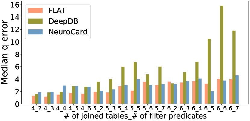
Figure 9. Q-error with different joining and predicate size.

E.4. End-to-End Test on JOB-ours Workload

We also perform the end-to-end test on Postgres using the harder workload JOB-ours. Since JOB-ours contains $1,500$ queries and the execution time of some queries is extremely long, we randomly sample $50$ queries from this workload for testing. The overall results are reported in Table 8.

Table 8. End-to-end testing results on JOB-ours workload.

		Average Query
Item	Algorithm	Time (Sec)	Improvement
Query Time	Postgres	431.7	—
Excluding	NeuroCard	379.2	$12.2\%$
CardEst	FLAT	383.3	$11.2\%$
Latency	True Cardinality	373.1	$13.6\%$
End-to-End	Postgres	432.3	—
Query	NeuroCard	405.7	$6.2\%$
Time	FLAT	386.9	$10.5\%$

We observe similar phenomenon on the JOB-ours workload. Specifically, for the query time excluding the CardEst query latency, the improvements of NeuroCard and our FLAT are close to the method using the true cardinality. For the end-to-end query time, the improvement of our FLAT is more significant than NeuroCard.

References

- (1)
- Armbrust et al. (2015) Michael Armbrust, Reynold S Xin, Cheng Lian, Yin Huai, Davies Liu, Joseph K Bradley, Xiangrui Meng, Tomer Kaftan, Michael J Franklin, Ali Ghodsi, et al. 2015. Spark sql: Relational data processing in spark. In SIGMOD. 1383–1394.
- Bottou (2012) Léon Bottou. 2012. Stochastic Gradient Descent Tricks. Neural networks: Tricks of the trade (2012), 421–436.
- Bruno et al. (2001) Nicolas Bruno, Surajit Chaudhuri, and Luis Gravano. 2001. STHoles: a multidimensional workload-aware histogram. In SIGMOD. 211–222.
- Chow and Liu (1968) C. Chow and Cong Liu. 1968. Approximating discrete probability distributions with dependence trees. IEEE transactions on Information Theory 14, 3 (1968), 462–467.
- Dagum and Luby (1993) Paul Dagum and Michael Luby. 1993. Approximating probabilistic inference in Bayesian belief networks is NP-hard. Artificial intelligence 60, 1 (1993), 141–153.
- Desana and Schnörr (2020) Mattia Desana and Christoph Schnörr. 2020. Sum–product graphical models. Machine Learning 109, 1 (2020), 135–173.
- Deshpande et al. (2001) Amol Deshpande, Minos Garofalakis, and Rajeev Rastogi. 2001. Independence is good: Dependency-based histogram synopses for high-dimensional data. ACM SIGMOD Record 30, 2 (2001), 199–210.
- Documentation 12 (2020) Postgresql Documentation 12. 2020. Chapter 70.1. Row Estimation Examples. https://www.postgresql.org/docs/current/row-estimation-examples.html (2020).
- Dutt et al. (2019) Anshuman Dutt, Chi Wang, Azade Nazi, Srikanth Kandula, Vivek Narasayya, and Surajit Chaudhuri. 2019. Selectivity estimation for range predicates using lightweight models. PVLDB 12, 9 (2019), 1044–1057.
- Fuchs et al. (2007) Dennis Fuchs, Zhen He, and Byung Suk Lee. 2007. Compressed histograms with arbitrary bucket layouts for selectivity estimation. Information Sciences 177, 3 (2007), 680–702.
- Gens and Pedro (2013) Robert Gens and Domingos Pedro. 2013. Learning the structure of sum-product networks. In ICML. PMLR, 873–880.
- Getoor et al. (2001) Lise Getoor, Benjamin Taskar, and Daphne Koller. 2001. Selectivity estimation using probabilistic models. In SIGMOD. 461–472.
- Graefe and Mckenna (1993) G. Graefe and W. J. Mckenna. 1993. The Volcano optimizer generator: extensibility and efficient search. In ICDE. 209–218.
- Gunopulos et al. (2000) Dimitrios Gunopulos, George Kollios, Vassilis J Tsotras, and Carlotta Domeniconi. 2000. Approximating multi-dimensional aggregate range queries over real attributes. In SIGMOD. 463–474.
- Gunopulos et al. (2005) Dimitrios Gunopulos, George Kollios, Vassilis J Tsotras, and Carlotta Domeniconi. 2005. Selectivity estimators for multidimensional range queries over real attributes. The VLDB Journal 14, 2 (2005), 137–154.
- Halford et al. (2019) Max Halford, Philippe Saint-Pierre, and Franck Morvan. 2019. An approach based on bayesian networks for query selectivity estimation. DASFAA 2 (2019).
- Hasan et al. (2019) Shohedul Hasan, Saravanan Thirumuruganathan, Jees Augustine, Nick Koudas, and Gautam Das. 2019. Multi-attribute selectivity estimation using deep learning. In SIGMOD.
- Heimel et al. (2015) Max Heimel, Martin Kiefer, and Volker Markl. 2015. Self-tuning, gpu-accelerated kernel density models for multidimensional selectivity estimation. In SIGMOD. 1477–1492.
- Hilprecht (2019) Benjamin Hilprecht. 2019. Github repository: deepdb public. https://github.com/DataManagementLab/deepdb-public (2019).
- Hilprecht et al. (2019) Benjamin Hilprecht, Andreas Schmidt, Moritz Kulessa, Alejandro Molina, Kristian Kersting, and Carsten Binnig. 2019. DeepDB: learn from data, not from queries!. In PVLDB.
- Ioannidis and Christodoulakis (1991) Yannis E Ioannidis and Stavros Christodoulakis. 1991. On the propagation of errors in the size of join results. In SIGMOD. 268–277.
- Khachatryan et al. (2015) Andranik Khachatryan, Emmanuel Müller, Christian Stier, and Klemens Böhm. 2015. Improving accuracy and robustness of self-tuning histograms by subspace clustering. IEEE TKDE 27, 9 (2015), 2377–2389.
- Kiefer et al. (2017) Martin Kiefer, Max Heimel, Sebastian Breß, and Volker Markl. 2017. Estimating join selectivities using bandwidth-optimized kernel density models. PVLDB 10, 13 (2017), 2085–2096.
- Kipf et al. (2019) Andreas Kipf, Thomas Kipf, Bernhard Radke, Viktor Leis, Peter Boncz, and Alfons Kemper. 2019. Learned cardinalities: Estimating correlated joins with deep learning. In CIDR.
- Kraska et al. (2018) Tim Kraska, Alex Beutel, Ed H Chi, Jeffrey Dean, and Neoklis Polyzotis. 2018. The case for learned index structures. In SIGMOD. 489–504.
- Krishna and Murty (1999) K Krishna and M Narasimha Murty. 1999. Genetic K-means algorithm. IEEE Transactions on Systems, Man, and Cybernetics, Part B (Cybernetics) 29, 3 (1999), 433–439.
- Krishnan et al. (2018) Sanjay Krishnan, Zongheng Yang, Ken Goldberg, Joseph Hellerstein, and Ion Stoica. 2018. Learning to optimize join queries with deep reinforcement learning. arXiv preprint arXiv:1808.03196 (2018).
- Leis et al. (2015) Viktor Leis, Andrey Gubichev, Atanas Mirchev, Peter Boncz, Alfons Kemper, and Thomas Neumann. 2015. How good are query optimizers, really? PVLDB 9, 3 (2015), 204–215.
- Leis et al. (2017) Viktor Leis, Bernhard Radke, Andrey Gubichev, Alfons Kemper, and Thomas Neumann. 2017. Cardinality Estimation Done Right: Index-Based Join Sampling. In CIDR.
- Leis et al. (2018) Viktor Leis, Bernhard Radke, Andrey Gubichev, Atanas Mirchev, Peter Boncz, Alfons Kemper, and Thomas Neumann. 2018. Query optimization through the looking glass, and what we found running the Join Order Benchmark. The VLDB Journal 27, 5 (2018), 643–668.
- Liang et al. (2020) Eric Liang, Zongheng Yang, Ion Stoica, Pieter Abbeel, Yan Duan, and Peter Chen. 2020. Variable Skipping for Autoregressive Range Density Estimation. In ICML. 6040–6049.
- Liu et al. (2015) Henry Liu, Mingbin Xu, Ziting Yu, Vincent Corvinelli, and Calisto Zuzarte. 2015. Cardinality estimation using neural networks. In Proceedings of the 25th Annual International Conference on Computer Science and Software Engineering. 53–59.
- Liu (2020) Luch Liu. 2020. Github repository: scikit-learn. https://github.com/scikit-learn/scikit-learn (2020).
- Lopes et al. (2019) Pedro Lopes, Craig Guyer, and Milener Gene. 2019. Sql docs: cardinality estimation (SQL Server). https://docs.microsoft.com/en-us/sql/relational-databases/performance/cardinality-estimation-sql-server?view=sql-server-ver15 (2019).
- Lopez-Paz et al. (2013) David Lopez-Paz, Philipp Hennig, and Bernhard Schölkopf. 2013. The randomized dependence coefficient. In NIPS. 1–9.
- Luan et al. (2020) Frank Luan, Amog Kamsetty, Eric Liang, and Zongheng Yang. 2020. Github repository: neurocard project. https://github.com/neurocard/neurocard (2020).
- Mao et al. (2019) Hongzi Mao, Malte Schwarzkopf, Shaileshh Bojja Venkatakrishnan, Zili Meng, and Mohammad Alizadeh. 2019. Learning scheduling algorithms for data processing clusters. In SIGCOMM. 270–288.
- Marcus et al. (2019) Ryan Marcus, Parimarjan Negi, Hongzi Mao, Chi Zhang, Mohammad Alizadeh, Tim Kraska, Olga Papaemmanouil, and Nesime Tatbul. 2019. Neo: A learned query optimizer. arXiv preprint arXiv:1904.03711 (2019).
- Martens and Medabalimi (2014) James Martens and Venkatesh Medabalimi. 2014. On the expressive efficiency of sum product networks. arXiv:1411.7717 (2014).
- McZgee and Carleton (1970) Victor E McZgee and Willard T Carleton. 1970. Piecewise regression. J. Amer. Statist. Assoc. 65, 331 (1970), 1109–1124.
- Nathan et al. (2020) Vikram Nathan, Jialin Ding, Mohammad Alizadeh, and Tim Kraska. 2020. Learning Multi-dimensional Indexes. In SIGMOD. 985–1000.
- New York (2020) State of New York. 2020. Vehicle, snowmobile, and boat registrations. https://catalog.data.gov/dataset/vehicle-snowmobile-and-boat-registrations (2020).
- Park et al. (2017) Yongjoo Park, Ahmad Shahab Tajik, Michael Cafarella, and Barzan Mozafari. 2017. Database learning: Toward a database that becomes smarter every time. In SIGMOD. 587–602.
- Perron et al. (2019) Matthew Perron, Zeyuan Shang, Tim Kraska, and Michael Stonebraker. 2019. How I learned to stop worrying and love re-optimization. In ICDE. 1758–1761.
- Poon and Domingos (2011) Hoifung Poon and Pedro Domingos. 2011. Sum-product networks: A new deep architecture. In ICCV Workshops. 689–690.
- Poosala and Ioannidis (1997) Viswanath Poosala and Yannis E Ioannidis. 1997. Selectivity estimation without the attribute value independence assumption. In VLDB, Vol. 97. 486–495.
- Rasmussen (2000) Carl Edward Rasmussen. 2000. The infinite Gaussian mixture model. In NIPS. 554–560.
- Reference Manual (2020) MySQL 8.0 Reference Manual. 2020. Chapter 15.8.10.2 Configuring Non-Persistent Optimizer Statistics Parameters. https://dev.mysql.com/doc/refman/8.0/en/innodb-statistics-estimation.html (2020).
- Repository (2020) UCI ML Repository. 2020. Gas sensor array temperature modulation Data Set. https://archive.ics.uci.edu/ml/datasets/Gas+sensor+array+temperature+modulation (2020).
- Scanagatta et al. (2019) Mauro Scanagatta, Antonio Salmerón, and Fabio Stella. 2019. A survey on Bayesian network structure learning from data. Progress in Artificial Intelligence (2019), 1–15.
- Selinger et al. (1979) P Griffiths Selinger, Morton M Astrahan, Donald D Chamberlin, Raymond A Lorie, and Thomas G Price. 1979. Access path selection in a relational database management system. In SIGMOD. 23–34.
- Server Documentation (2020) MariaDB Server Documentation. 2020. Statistics for optimizing queries: InnoDB persistent statistics. https://mariadb.com/kb/en/innodb-persistent-statistics/ (2020).
- Sethi et al. (2019) Raghav Sethi, Martin Traverso, Dain Sundstrom, David Phillips, Wenlei Xie, Yutian Sun, Nezih Yegitbasi, Haozhun Jin, Eric Hwang, Nileema Shingte, et al. 2019. Presto: Sql on everything. In ICDE. 1802–1813.
- Srivastava et al. (2006) Utkarsh Srivastava, Peter J Haas, Volker Markl, Marcel Kutsch, and Tam Minh Tran. 2006. Isomer: Consistent histogram construction using query feedback. In ICDE. 39–39.
- Stillger et al. (2001) Michael Stillger, Guy M Lohman, Volker Markl, and Mokhtar Kandil. 2001. LEO-DB2’s learning optimizer. In PVLDB, Vol. 1. 19–28.
- Thirumuruganathan et al. (2020) Saravanan Thirumuruganathan, Shohedul Hasan, Nick Koudas, and Gautam Das. 2020. Approximate query processing for data exploration using deep generative models. In ICDE. 1309–1320.
- Tzoumas et al. (2011) Kostas Tzoumas, Amol Deshpande, and Christian S Jensen. 2011. Lightweight graphical models for selectivity estimation without independence assumptions. PVLDB 4, 11 (2011), 852–863.
- Van Aken et al. (2017) Dana Van Aken, Andrew Pavlo, Geoffrey J Gordon, and Bohan Zhang. 2017. Automatic database management system tuning through large-scale machine learning. In SIGMOD. 1009–1024.
- Wang and Sevcik (2003) Hai Wang and Kenneth C Sevcik. 2003. A multi-dimensional histogram for selectivity estimation and fast approximate query answering. In Proceedings of the 2003 conference of the Centre for Advanced Studies on Collaborative research. 328–342.
- Wang et al. (2020) Xiaoying Wang, Changbo Qu, Weiyuan Wu, Jiannan Wang, and Qingqing Zhou. 2020. Are we ready for learned cardinality estimation? arXiv:2012.06743 [cs.DB]
- Wu et al. (2018) Chenggang Wu, Alekh Jindal, Saeed Amizadeh, Hiren Patel, Wangchao Le, Shi Qiao, and Sriram Rao. 2018. Towards a learning optimizer for shared clouds. PVLDB 12, 3 (2018), 210–222.
- Yang et al. (2021) Zongheng Yang, Amog Kamsetty, Sifei Luan, Eric Liang, Yan Duan, Xi Chen, and Ion Stoica. 2021. NeuroCard: One Cardinality Estimator for All Tables. PVLDB 14, 1 (2021), 61–73.
- Yang et al. (2019) Zongheng Yang, Eric Liang, Amog Kamsetty, Chenggang Wu, Yan Duan, Xi Chen, Pieter Abbeel, Joseph M Hellerstein, Sanjay Krishnan, and Ion Stoica. 2019. Deep unsupervised cardinality estimation. PVLDB (2019).
- Yang and Wu (2019) Zongheng Yang and Chenggang Wu. 2019. Github repository: naru project. https://github.com/naru-project/naru (2019).
- Zhao et al. (2018) Zhuoyue Zhao, Robert Christensen, Feifei Li, Xiao Hu, and Ke Yi. 2018. Random sampling over joins revisited. In SIGMOD. 1525–1539.
- Zhu et al. (2020) Rong Zhu, Ziniu Wu, Yuxing Han, Kai Zeng, Andreas Pfadler, Zhengping Qian, Jingren Zhou, and Bin Cui. 2020. FLAT: Fast, Lightweight and Accurate Method for Cardinality Estimation [Technical Report]. arXiv preprint arXiv:2011.09022 (2020).