A Novel RIS-Assisted Modulation Scheme

Abstract

In this work, in order to achieve higher spectrum efficiency, we propose a reconfigurable intelligent surface (RIS)-assisted multi-user communication uplink system. Different from previous work in which the RIS only optimizes the phase of the incident users’s signal, we propose the use of the RIS to create a virtual constellation diagram to transmit the data of an additional user signal. We focus on the two-user case and develop a tight approximation for the cumulative distribution function (CDF) of the received signal-to-noise ratio of both users. Then, based on the proposed statistical distribution, we derive the analytical expressions of the average bit error rate of the considered two users. The paper shows the trade off between the performance of the two users against each other as a function of the proposed phase shift at the RIS.

I Introduction

Reconfigurable intelligent surfaces (RISs) are man-made surfaces composed of electromagnetic (EM) materials, which are highly controllable by leveraging electronic devices. In essence, an RIS can deliberately control the reflection/scattering characteristics of the incident wave to enhance the signal quality at the receiver, and hence converts the propagation environment into a smart one [1].

Owing to their promising gains, recently RISs have been extensively investigated in the literature. In particular, the authors in [2] proposed a practical phase shift model for RISs. In [3], the authors studied the beamforming optimization of RIS-assisted wireless communication under the constraints of discrete phase shifts, while in [4], the authors studied the coverage and signal-to-noise ratio (SNR) gain of RIS-assisted communication systems. In [5], the authors proposed highly accurate closed-form approximations to channel distributions of two different RIS-based wireless system setups. Recently, RISs have been used in many scenarios and have shown superior performance over systems not employing RISs. For instance, in [6], an intelligent reflecting surface (IRS)-assisted multiple-input single-output communication system is considered, and in [7], the physical layer security of RIS-assisted communication with an eavesdropping user is studied. In [8], the authors proposed RIS-assisted dual-hop unmanned aerial vehicle (UAV) communication systems while in [9], the authors used the RIS for downlink multi-user communication from a multi-antenna base station, and developed an energy-efficient designs for transmit power allocation and phase shifts of the surface reflection elements.

In all of the above studies, the advantages of RISs are mainly used to enhance the quality of the signal, and the reflection patterns were not used to carry additional information. i.e., the role of an RIS has been mainly based on the mitigation of the phase shifts of the involved channels, without any additional purpose of controlling those phase shifts. In this paper, we propose a novel modulation scheme utilizing the phase shifts of the RIS in a spectrally efficient way to superimpose the data of an additional user 2 (U2) on that of the ordinary user 1 (U1).

More specifically, we consider a multi-user uplink scenario and mainly consider the feasibility of uploading the data of two users simultaneously through the RIS, where U1 sends the data to the base station through a direct link and is given a chance to utilize an available RIS-assisted link to enhance its signal, but with the condition of having the data of U2 embedded with its data through the RIS. Basically, the RIS optimizes the phase of the incident U1’s signal to mitigate the phase shifts of the cascaded link as well as its direct link, and additionally to embed the data of U2 through creating a modified virtual constellation diagram. Hence, we assume that U2’s data is known when the RIS optimizes the phase of the incident U1’s signal, and then, a virtual constellation diagram is created by the RIS to embed U2’s data. Consequently, the signal reflected by the RIS contains the data of both users. In summary, the main contributions of this work include the following: (i) we propose a novel and spectrallly efficient RIS-assisted modulation scheme, (ii) for the proposed system, we develop two tight approximate statistical distributions for the received SNR of the two considered users, (iii) based on the proposed statistical distributions, closed-form expressions for the average bit error rates (BER) are derived and analysed.

The remaining of this letter is organized as follows. Section II presents the system and channel models. The performance analysis is presented in section III, and the numerical and simulation results are detailed in section IV. Finally, conclusions are drawn in section V.

II System and Channel Models

We consider the uplink system shown in Fig. 1, where U1 is communicating with the base station (BS) directly and with the help of an RIS to boost its connectivity. In the same time, U2 is in the vicinity of the RIS and is communicating with the BS through superimposing its signal on that of U1 using the RIS. It is assumed that the RIS can obtain perfect channel state information (CSI) through a control link that enables it to optimize the phase shifts of the reflected signals. As will be discussed later, the phase shifts will be utilized to superimpose U2 data on that of U1 in a way to efficiently utilize the same spectrum. This is in return of allowing U1 to take advantage of the RIS to improve its connectivity to the BS. At the receiving end, the BS first decodes the signal of U1 and extracts it from the composite received signal. In the second step, the remaining signal is processed to get the data of U2.

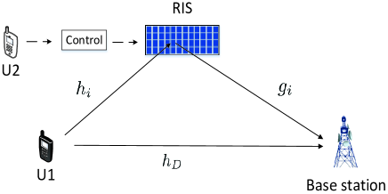
Figure 1: RIS-assisted multi-user uplink.

II-A Analysis of User 1 SNR

As mentioned above, U1 is communicating with the BS through the RIS-assisted dual-hop link and a direct link. A binary phase shift keying (BPSK) symbol $x$ with average power $E_{s}$ is sent to the RIS with $N$ reflecting elements through a set of channels $h_{i}=\alpha_{i}e^{j\theta_{i}}$ where $\alpha_{i}$’s are independent and identically distributed (i.i.d.) Rayleigh random variables (RVs) with mean $\sqrt{\pi}/2$, variance $(4-\pi)/4$, and uniformly distributed phase $\theta_{i}$. Meanwhile, the direct link to the BS is denoted as $h_{D}=\varepsilon e^{j\eta}$, where $\varepsilon$ is a Rayleigh random variable (RV) with mean $\sqrt{\pi}/2$, variance $(4-\pi)/4$ and phase $\eta$. The RIS elements are assumed to have a line of sight with the BS through channels $g_{i}=\beta_{i}e^{j\psi_{i}}$ where $\beta_{i}$ are i.i.d. Rician RVs with Rician factor $K$ and phases $\psi_{i}$. With the knowledge of the different channels CSI (U1-RIS, RIS-BS, U1-BS), the RIS optimizes the incident signals in a way to create a virtual constellation diagram by embedding the signal of U2. The overall received signal at the BS including that of the direct link can be expressed as

$$y_{1} =\left(\sqrt{\frac{E_{s}}{L_{1}}}h_{D}+\sqrt{\frac{E_{s}}{L_{2}}}\sum_{i=1}^{N}h_{i}g_{i}{\rm{e}}^{j\phi_{i}}\right)x+n$$

$$=\left(\sqrt{\frac{E_{s}}{L_{1}}}\varepsilon+\sqrt{\frac{E_{s}}{L_{2}}}\sum_{i=1}^{N}\alpha_{i}\beta_{i}{\rm{e}}^{jw_{m}}\right)x+n,$$ (1)

where $L_{1}$ and $L_{2}$ are the path losses of the direct link and the RIS-assisted dual-hop link, respectively, $\phi_{i}=(w_{m}-\theta_{i}-\psi_{i}+\eta)$ is the adjustable phase introduced by the $i$th reflecting element of the RIS to mitigate the channels’ phase shifts, $w_{m}$ is the message-dependent phase introduced by the RIS to carry the information of U2 where $w_{m}$ represents a binary symbol of 1 and $-w_{m}$ represents 0, and $n\sim\mathcal{C}\mathcal{N}(0,N_{0})$ is the additive white Gaussian noise (AWGN) signal.

Then, the received SNR can be written as

$$\gamma_{1}= \frac{\left(\sqrt{\frac{E_{s}}{L_{1}}}\varepsilon+\sqrt{\frac{E_{s}}{L_{2}}}\sum_{i=1}^{N}\alpha_{i}\beta_{i}\cos(w_{m})\right)^{2}}{N_{0}}$$

$$= \left(\sqrt{\bar{\gamma}_{1}}\varepsilon+\sqrt{\bar{\gamma}_{2}}R_{1}\right)^{2}=Z_{1}^{2},$$ (2)

where $R_{1}=\sum_{i=1}^{N}\alpha_{i}\beta_{i}\cos(w_{m})$ , $\bar{\gamma}_{1}={\bar{\gamma}}/{L_{1}}$, $\bar{\gamma}_{2}={\bar{\gamma}}/{L_{2}}$ and $\bar{\gamma}=E_{s}/N_{0}$ denotes the average SNR.

For a sufficiently large number of reflecting elements $N$, and relying on the central limit theorem (CLT), $R_{1}$ can be assumed to follow a Gaussian RV. Thus, the probability density function (PDF) of $R_{1}$ can be simply expressed as

$$f_{R_{1}}(r)=\frac{1}{\sqrt{2\pi\sigma_{1}^{2}}}\exp\left(-\frac{\left(r-\mu_{1}\right)^{2}}{2\sigma_{1}^{2}}\right),$$ (3)

where $\mu_{1}=\frac{N\Gamma\left(\frac{3}{2}\right)\sqrt{\pi}}{2\sqrt{1+K}e^{K}}{}_{1}F_{1}(\frac{3}{2},1,K)\cos(w_{m})$, $\sigma_{1}^{2}=N\left[\frac{{}_{1}{\rm{F}}_{1}(2,1,K)}{(1+K)e^{K}}-\left(\frac{\mu_{1}}{N\cos(w_{m})}\right)^{2}\right]\cos^{2}(w_{m})$, ${}_{1}F_{1}(\cdot)$ is the Degenerate hypergeometric function, and $\Gamma(\cdot)$ is the Gamma function [10]. Then, we obtain the cumulative distribution function (CDF) of $Z_{1}$ as

$$F_{Z_{1}}(z) =\Pr(\sqrt{\bar{\gamma}_{1}}\varepsilon+\sqrt{\bar{\gamma}_{2}}R_{1}<Z)$$

$$=\int_{0}^{\frac{z}{\sqrt{\bar{\gamma}_{2}}}}\frac{1}{\sqrt{2\pi\sigma_{1}^{2}}}\exp\left(-\frac{\left(r-\mu_{1}\right)^{2}}{2\sigma_{1}^{2}}\right)dr$$

$$-\int_{0}^{\frac{z}{\sqrt{\bar{\gamma}_{2}}}}\frac{1}{\sqrt{2\pi\sigma_{1}^{2}}}{\rm{e}}^{\left(-\frac{\left(r-\mu_{1}\right)^{2}}{2\sigma_{1}^{2}}-\frac{\left(z-\sqrt{\bar{\gamma}_{2}}r\right)^{2}}{\bar{\gamma}_{1}}\right)}dr.$$ (4)

From [10, Eq.(2.33.1)], the CDF of $\gamma_{1}$ is given by

$$F_{\gamma_{1}}(\gamma)=\frac{1}{2}\left[\rm{erf}\left(\frac{C_{2}\sqrt{\gamma}-\mu_{1}}{\sqrt{2\sigma_{1}^{2}}}\right)+\rm{erf}\left(\frac{\mu_{1}}{\sqrt{2\sigma_{1}^{2}}}\right)\right]$$

$$-\frac{1}{2\sqrt{2}C_{3}}\rm{e}^{\left(-\frac{\left(C_{1}C_{2}\sqrt{\gamma}-C_{1}\mu_{1}\right)^{2}}{2C_{3}^{2}C_{2}^{2}}\right)}\left[\rm{erf}\left(\frac{C_{2}\sqrt{\gamma}-\mu_{1}}{2C_{3}\sigma_{1}}\right)\right]$$

$$-\frac{1}{2\sqrt{2}C_{3}}\rm{e}^{\left(-\frac{\left(C_{1}C_{2}\sqrt{\gamma}-C_{1}\mu_{1}\right)^{2}}{2C_{3}^{2}C_{2}^{2}}\right)}\left[\rm{erf}\left(\frac{C_{4}\sqrt{\gamma}+\mu_{1}}{2C_{3}\sigma_{1}}\right)\right],$$ (5)

where $C_{1}=\frac{1}{\sqrt{\bar{\gamma}_{1}}}$, $C_{2}=\frac{1}{\sqrt{\bar{\gamma}_{2}}}$,$C_{3}=\sqrt{\frac{\sigma^{2}L_{1}}{L_{2}}+\frac{1}{2}}$, $C_{4}=\frac{2\sigma_{1}^{2}C_{1}^{2}}{C_{2}}$ and ${\rm{erf}}(\cdot)$ is the error function [10].

$$A_{2}{=}\sqrt{\frac{\bar{\gamma}_{1}\gamma}{2\sigma_{2}^{2}\bar{\gamma}_{2}{+}\bar{\gamma}_{1}\gamma}}\exp\left(\frac{1}{\bar{\gamma}_{1}}{-}\frac{\mu_{2}^{2}}{2\sigma_{2}^{2}}\right)\left[\sum_{l=0}^{L}\sum_{k=0}^{l-1}\frac{(\gamma\mu_{2}^{2})^{l}\left(\frac{1}{2}{-}l\right)_{l{-}k{-}1}({-}1)^{l{+}k{-}1}\left(\frac{1}{\bar{\gamma}_{1}}{+}\frac{\gamma}{2\bar{\gamma}_{2}\sigma_{2}^{2}}\right)^{k{+}\frac{1}{2}}}{l!2^{l}\Gamma(l{+}\frac{1}{2})\left(\gamma\sigma_{2}^{2}{+}\frac{2\bar{\gamma}_{2}\sigma_{2}^{4}}{\bar{\gamma}_{1}}\right)^{l}\exp\left(\frac{1}{\bar{\gamma}_{1}}{+}\frac{\gamma}{2\bar{\gamma}_{2}\sigma_{2}^{2}}\right)}{+}\sum_{l=0}^{L}\frac{(\gamma\mu_{2}^{2})^{l}{\rm{erfc}}\left(\frac{1}{\bar{\gamma}_{1}}{+}\frac{\gamma}{2\bar{\gamma}_{2}\sigma_{2}^{2}}\right)}{l!2^{l}\left(\gamma\sigma_{2}^{2}{+}\frac{2\bar{\gamma}_{2}\sigma_{2}^{4}}{\bar{\gamma}_{1}}\right)^{l}}\right]$$ (12)

$$I_{1}= \frac{\sqrt{\pi}}{2}\left[1+{\rm{erf}}(\frac{\mu_{1}}{\sqrt{2\sigma_{1}^{2}}})-2{\rm{erf}}(\frac{\mu_{1}}{C_{2}})\right]+\sum_{i=1}^{4}\frac{S_{i}}{2}\sqrt{\frac{2\pi\sigma_{1}^{2}}{2\sigma_{1}^{2}+T_{i}C_{2}^{2}}}\exp(\frac{T_{i}^{2}C_{2}^{2}\mu_{1}^{2}}{4\sigma_{1}^{4}+2T_{i}C_{2}^{2}\sigma_{1}^{2}}-\frac{T_{i}\mu_{1}^{2}}{2\sigma_{1}^{2}})$$

$$\times\left[2{\rm{erf}}\left(\sqrt{\frac{\mu_{1}^{2}}{C_{2}^{2}}+\frac{T_{i}^{2}\mu_{1}^{2}}{2\sigma_{1}^{2}}}-\frac{T_{i}C_{2}\mu_{1}}{\sqrt{4\sigma_{1}^{4}+2T_{i}C_{2}^{2}\sigma_{1}^{2}}}\right)-{\rm{erfc}}\left(\frac{T_{i}C_{2}\mu_{1}}{\sqrt{4\sigma_{1}^{4}+2T_{i}C_{2}^{2}\sigma_{1}^{2}}}\right)\right]$$ (16)

$$I_{2}= \frac{1}{2}\sqrt{\frac{\pi}{2C_{3}^{2}+C_{1}^{2}}}\exp\left(-\frac{\mu_{1}^{2}C_{1}^{2}}{2C_{2}^{2}C_{3}^{2}+C_{1}^{2}C_{2}^{2}}\right)\left(1+\rm{erf}\left(\frac{C_{1}^{2}\mu_{1}}{\sqrt{4C_{2}^{2}C_{3}^{4}+2C_{1}^{2}C_{2}^{2}C_{3}^{2}}}\right)\right)$$

$$-\sum_{i=1}^{4}\frac{S_{i}}{\sqrt{2}}\sqrt{\frac{\pi\sigma_{1}^{2}}{4C_{3}^{2}\sigma_{1}^{2}+2C_{1}^{2}\sigma_{1}^{2}+T_{i}C_{4}^{2}}}\exp\left(C_{5}-\frac{\mu_{1}^{2}C_{1}^{2}}{2C_{2}^{2}C_{3}^{2}}-\frac{\mu_{1}^{2}T_{i}}{4C_{3}^{2}\sigma_{1}^{2}}\right)\left(1+{\rm{erf}}\left(\sqrt{C_{5}}\right)\right)$$ (17)

$$I_{3}= \frac{1}{2}\sqrt{\frac{\pi}{2C_{3}^{2}+C_{1}^{2}}}\exp\left(-\frac{\mu_{1}^{2}C_{1}^{2}}{2C_{2}^{2}C_{3}^{2}+C_{1}^{2}C_{2}^{2}}\right)\left[{\rm{erfc}}\left(\frac{\mu_{1}C_{1}^{2}}{\sqrt{4C_{2}^{2}C_{3}^{4}+2C_{1}^{2}C_{2}^{2}C_{3}^{2}}}\right)-2{\rm{erf}}\left(\sqrt{C_{7}}-\frac{\mu_{1}C_{1}^{2}}{\sqrt{4C_{2}^{2}C_{3}^{4}+2C_{1}^{2}C_{2}^{2}C_{3}^{2}}}\right)\right]$$

$$+\sum_{i=1}^{4}\frac{S_{i}}{\sqrt{2}}\sqrt{\frac{\pi\sigma_{1}^{2}}{4C_{3}^{2}\sigma_{1}^{2}+2C_{1}^{2}\sigma_{1}^{2}+T_{i}C_{2}^{2}}}\exp\left(C_{6}-\frac{C_{1}^{2}\mu_{1}^{2}}{2C_{2}^{2}C_{3}^{2}}-\frac{T_{i}\mu_{1}^{2}}{4C_{3}^{2}\sigma_{1}^{2}}\right)\left[2{\rm{erf}}\left(\sqrt{C_{7}}-\sqrt{C_{6}}\right)-{\rm{erfc}}\left(\sqrt{C_{6}}\right)\right]$$ (18)

II-B Analysis of User 2 SNR

Assuming that the signal of U1 can be successfully decoded (represented by $\hat{x}$), the received signal can now be expressed as

$$y_{2} =y_{1}{\rm{e}}^{j\hat{x}\pi}$$

$$=\sqrt{\frac{E_{s}}{L_{2}}}\sum_{i=1}^{N}\alpha_{i}\beta_{i}{\rm{e}}^{jw_{m}}x{\rm{e}}^{j\hat{x}\pi}+\sqrt{\frac{E_{s}}{L_{1}}}\varepsilon x{\rm{e}}^{j\hat{x}\pi}+n{\rm{e}}^{j\hat{x}\pi}$$

$$=\sqrt{\frac{E_{s}}{L_{2}}}\sum_{i=1}^{N}\alpha_{i}\beta_{i}{\rm{e}}^{jw_{m}}+\sqrt{\frac{E_{s}}{L_{1}}}\varepsilon+n{\rm{e}}^{j\hat{x}\pi}.$$ (6)

Thus, the signal of U2 can be regarded as a biased BPSK signal with an initial phase of $\frac{\pi}{2}$, and an offset angle of $\frac{\pi}{2}-w_{m}$. Then, the SNR of U2 can be written as

$$\gamma_{2}=\frac{\frac{\bar{\gamma}}{L_{2}}\left(\sum_{i=1}^{N}\alpha_{i}\beta_{i}\cos(\frac{\pi}{2}-w_{m})\right)^{2}}{\frac{\bar{\gamma}}{L_{1}}\left|\varepsilon\right|^{2}+1}\ =\frac{\bar{\gamma}_{2}R_{2}^{2}}{\bar{\gamma}_{1}\left|\varepsilon\right|^{2}+1}.$$ (7)

where $R_{2}=\sum_{i=1}^{N}\alpha_{i}\beta_{i}\cos(\frac{\pi}{2}-w_{m})$. Similar to $R_{1}$, and relying again on the CLT, $R_{2}$ is assumed to follow the Gaussian distribution with mean $\mu_{2}$ and variance $\sigma_{2}^{2}$. The PDF of $R_{2}$ can be written as

$$f_{R_{2}}(r)=\frac{1}{\sqrt{2\pi\sigma_{2}^{2}}}\exp\left(-\frac{\left(r-\mu_{2}\right)^{2}}{2\sigma_{2}^{2}}\right),$$ (8)

where $\mu_{2}=\frac{N\Gamma\left(\frac{3}{2}\right)\sqrt{\pi}}{2\sqrt{1+K}e^{K}}{}_{1}F_{1}(\frac{3}{2},1,K)\cos(\frac{\pi}{2}-w_{m})$, and $\sigma_{2}^{2}=N\left[\frac{{}_{1}{\rm{F}}_{1}(2,1,K)}{(1+K)e^{K}}-\left(\frac{\mu_{1}}{N\cos(\frac{\pi}{2}-w_{m})}\right)^{2}\right]\cos^{2}(\frac{\pi}{2}-w_{m})$.

Let $Y=\bar{\gamma}_{1}\left|\varepsilon\right|^{2}+1$, then the PDF of $Y$ can be readily written as $f_{Y}(y)=\frac{1}{\bar{\gamma}_{1}}e^{-\frac{y-1}{\bar{\gamma}_{1}}}$. Thus the CDF of $\gamma_{2}$ can be calculated as

$$F_{\gamma_{2}}(\gamma)= \Pr\left(\frac{\bar{\gamma}_{2}R_{2}^{2}}{Y}<\gamma\right)$$

$$= 1-Q_{\frac{1}{2}}\left(\frac{\mu_{2}}{\sqrt{\sigma_{2}^{2}}},\sqrt{\frac{\gamma}{\sigma_{2}^{2}\bar{\gamma}_{2}}}\right)$$

$$+\sqrt{\frac{\bar{\gamma}_{1}\gamma}{2\sigma_{2}^{2}\bar{\gamma}_{2}+\bar{\gamma}_{1}\gamma}}\exp\left(\frac{1}{\bar{\gamma}_{1}}-\frac{\mu_{2}^{2}\bar{\gamma}_{2}}{\bar{\gamma}_{1}\gamma+2\sigma_{2}^{2}\bar{\gamma}_{2}}\right)$$

$$\times Q_{\frac{1}{2}}\left(\sqrt{\frac{\mu_{2}^{2}\gamma}{\sigma_{2}^{2}\gamma+\frac{2\bar{\gamma}_{2}\sigma_{2}^{4}}{\bar{\gamma}_{1}}}},\sqrt{\frac{2}{\bar{\gamma}_{1}}+\frac{\gamma}{\bar{\gamma}_{2}\sigma_{2}^{2}}}\right),$$ (9)

where $Q_{\frac{1}{2}}(\cdot,\cdot)$ is the Marcum Q-function [10].

Using (9) to calculate the average BER is difficult, however, from [11, Eq. (16)], we have

$$Q_{\frac{1}{2}}\left(a,b\right)\approx\sum_{l=0}^{L}\frac{a^{2l}\Gamma(l+\frac{1}{2},\frac{b^{2}}{2})}{l!\Gamma(l+\frac{1}{2})2^{l}{\rm{e}}^{\frac{a^{2}}{2}}},$$ (10)

where $\Gamma(\cdot,\cdot)$ is the incomplete gamma function [10]. Then, with the help of [12, Eq. (06.06.03.0005.01)], the CDF of $\gamma_{2}$ can be written as

$$F_{\gamma_{2}}(\gamma)\approx A_{1}+A_{2},$$ (11)

where $A_{1}=1-\sum_{l=0}^{L}\frac{(\frac{\mu_{2}}{\sigma_{2}})^{2l}\Gamma(l+\frac{1}{2},\frac{\gamma}{2\bar{\gamma}_{2}\sigma_{2}^{2}})}{l!\Gamma(l+\frac{1}{2})2^{l}{\rm{exp}}({\frac{\mu^{2}}{2\sigma_{2}^{2}}})}$, $A_{2}$ is shown at the bottom of this page, and $\rm{erfc}(\cdot)$ is the complementary error function [10].

$$I_{4}= \Gamma\left(\frac{1}{2}\right)-\sum_{l=0}^{L}\left(\frac{\left(\frac{\mu_{2}^{2}}{\sigma_{2}^{2}}\right)^{l}\sqrt{2\bar{\gamma}_{2}\sigma_{2}^{2}}}{2^{l-1}\Gamma(l+\frac{1}{2})e^{\frac{\mu_{2}^{2}}{2\sigma_{2}^{2}}}(1+2\bar{\gamma}_{2}\sigma_{2}^{2})^{1+l}}{}_{2}{\rm{F}}_{1}\left(1,l+1;\frac{3}{2};\frac{2\bar{\gamma}_{2}\sigma_{2}^{2}}{1+2\bar{\gamma}_{2}\sigma_{2}^{2}}\right)\right)$$ (21)

$$I_{5}= \exp\left(\frac{1}{\bar{\gamma}_{1}}-\frac{\mu_{2}^{2}}{2\sigma_{2}^{2}}\right)\sum_{l=0}^{L}\sum_{i=1}^{4}\frac{S_{i}(\frac{\mu_{2}}{\sigma_{2}})^{2l}}{2^{l}(1+\frac{T_{i}}{2\bar{\gamma}_{2}\sigma_{2}^{2}})^{3/4}(\frac{2\bar{\gamma}_{2}\sigma_{2}^{2}}{\bar{\gamma}_{1}})^{1/4}}\exp\left(\frac{\bar{\gamma}_{2}\sigma_{2}^{2}}{\bar{\gamma}_{1}}-\frac{T_{i}}{2\bar{\gamma}_{1}}\right){\rm{W}}_{-l-\frac{1}{4},-\frac{1}{4}}\left(\frac{2\bar{\gamma}_{2}\sigma_{2}^{2}}{\bar{\gamma}_{1}}+\frac{T_{i}}{\bar{\gamma}_{1}}\right)$$ (22)

$$I_{6}= \exp\left(\frac{1}{\bar{\gamma}_{1}}-\frac{\mu_{2}^{2}}{2\sigma_{2}^{2}}\right)\sum_{l=0}^{L}\sum_{k=1}^{l-1}\frac{\mu_{2}^{2l}(\bar{\gamma}_{2}\sigma_{2}^{2})^{k/2}\left(\frac{1}{2}-l\right)_{l-k-1}(-1)^{k+l-1}}{\Gamma(l+\frac{1}{2})2^{l}\sigma_{2}^{2l}(\bar{\gamma}_{2}\bar{\gamma}_{1}\sigma_{2}^{2})^{k+\frac{1}{2}}\sqrt{\bar{\gamma}_{1}/2}}\exp\left(\frac{\bar{\gamma}_{2}\sigma_{2}^{2}}{\bar{\gamma}_{1}}-\frac{1}{2\bar{\gamma}_{1}}\right)\left(\frac{2}{\bar{\gamma}_{1}}+\frac{1}{\bar{\gamma}_{2}\bar{\gamma}_{1}\sigma_{2}^{2}}\right)^{-k/2-1}$$

$$\times{\rm{W}}_{\frac{k-2l}{2},\frac{-k-1}{2}}\left(\frac{2\bar{\gamma}_{2}\sigma_{2}^{2}}{\bar{\gamma}_{1}}+\frac{1}{\bar{\gamma}_{1}}\right)$$ (23)

III Performance Analysis

In this section, we analyze the performance of the proposed scheme by deriving closed-form expressions for the average BER. For different binary modulation schemes, a unified average BER expression is given by [13]

$$P_{e}=\frac{q^{p}}{2\Gamma(p)}\int_{0}^{\infty}\exp(-q\gamma)\gamma^{p-1}F_{\gamma}(\gamma)d\gamma,$$ (13)

where $F_{\gamma}(\gamma)$ is the CDF of $\gamma$, and the parameters $p$ and $q$ are modulation schemes dependent. In this work, we consider BPSK modulation, and hence we use $p=\frac{1}{2}$ and $q$ = 1.

III-1 Average BER of User 1

From (5) and (13), $P_{e1}$ can be formulated as

$$P_{e1}=(I_{1}-I_{2}-I_{3})/(2\Gamma(0.5)),$$ (14)

where $I_{1}$, $I_{2}$ and $I_{3}$ are derived next. Using the expression in (5) to evaluate $P_{e1}$ is difficult. Hence, we opt to utilize an alternative expression for the erf function [14] as

$$\begin{split}\rm{erf}(x)\approx\left\{\begin{matrix}1-\sum_{i=1}^{4}S_{i}{\rm{e}}^{-T_{i}x^{2}}x\geq 0\\ -1+\sum_{i=1}^{4}S_{i}{\rm{e}}^{-T_{i}x^{2}}x<0\end{matrix}\right.\end{split}$$ (15)

where $S=[\frac{1}{8},\frac{1}{4},\frac{1}{4},\frac{1}{4}]$ and $T=[1,2,\frac{20}{3},\frac{20}{17}]$.

Then, with the help of [10, Eq. (2.33.1)], closed form expressions for $I_{1}$, $I_{2}$, and $I_{3}$ are shown at the bottom of the previous page, where $C_{5}=\frac{\left(2C_{1}^{2}\mu_{1}\sigma_{1}^{2}-T_{i}C_{2}C_{4}\mu_{1}\right)^{2}}{16C_{2}^{2}C_{3}^{4}\sigma_{1}^{4}+8C_{1}^{2}C_{2}^{2}C_{3}^{2}\sigma_{1}^{4}+4T_{i}C_{2}^{2}C_{3}^{2}C_{4}^{2}\sigma_{1}^{2}}$, $C_{6}=\frac{\left(2C_{1}^{2}\mu_{1}\sigma_{1}^{2}+T_{i}C_{2}^{2}\mu_{1}\right)^{2}}{16C_{2}^{2}C_{3}^{4}\sigma_{1}^{4}+8C_{1}^{2}C_{2}^{2}C_{3}^{2}\sigma_{1}^{4}+4T_{i}C_{2}^{4}C_{3}^{2}\sigma_{1}^{2}}$, and $C_{7}=\frac{\mu_{1}^{2}}{C_{2}^{2}}+\frac{\mu_{1}^{2}C_{1}^{2}}{2C_{2}^{2}C_{3}^{2}}$.

III-2 Average BER of User 2

As the decoding of U2 signal follows that of U1, it is usually difficult to ensure that the decoded signal is completely correct. Therefore, after processing the received signal, we might get some inverted information bits of U2. Then, the practical average BER of U2 can be expressed as

$$P_{e2}=P_{e2}^{ideal}(1-P_{e1})+P_{e1}(1-P_{e2}^{ideal}),$$ (19)

where $P_{e2}^{ideal}$ denotes U2’s average BER with ideal conditions (i.e. assuming the decoded U1’s data is completely correct). From (11) and (13), and using [10, Eq. (6.455)], the ideal U2’s average BER can be calculated as

$$P_{e2}^{ideal}=(I_{4}+I_{5}+I_{6})/(2\Gamma(0.5)),$$ (20)

where $I_{4}$, $I_{5}$ and $I_{6}$ can be shown to be given as in (21), (22) and (23), where ${}_{2}F_{1}(\cdot)$ is the Gauss hypergeometric function, and $W_{a,b}(\cdot)$ is the Whittaker hypergeometric function [10].

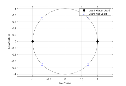
Figure 2: The constellation diagram of U1 and U2.

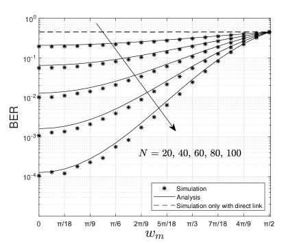
Figure 3: Average BER of U1 versus $w_{m}$.

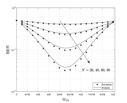
Figure 4: Average BER of U2 versus $w_{m}$.

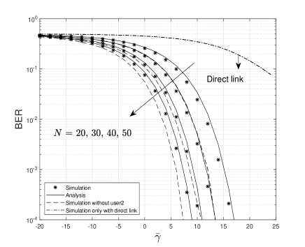
Figure 5: Average BER of U1 versus $\bar{\gamma}$ with and without U2.

IV Numerical and Simulation Results

In this section, we present some numerical results to verify our analysis. The parameters used in the figures are $k$ = 3, $p=\frac{1}{2}$, $q=1$, $L_{1}=20$ dB, and $L_{3}=30$ dB.

In Fig. 2 we plot the constellation diagram of U1 and U2 where $\bar{\gamma}=20$ dB, $N=50$ and $w_{m}=\pi/4$. It can be deduced from Fig. 2 that superimposing U2’s data on that of U1 causes the constellation diagram of U1’s to shift based on the value of $w_{m}$ used. This causes the BER of U1 to increase, simply because the separation of the two constellation points is lower at this time. From the constellation of U2, it can be deduced that the processed signal is similar to a BPSK signal where the initial phase is $-\pi/2$.

In Fig. 3, we plot the average BER of U1 as a function of $w_{m}$. When $w_{m}=0$, this is equivalent to the case where there is no U2 and only the data of U1 is transmitted in the uplink, and its constellation is a pure BPSK one. As we increase $w_{m}$, the system needs to utilize the spectrum resources of U1 to transmit the signal of U2. Consequently, U1’s average BER increases. When $w_{m}$ reaches $\pi/2$, it leads to the lowest data accuracy of U1. In addition, and as expected, it can be seen from Fig. 3 that increasing $N$ can bring performance improvements to U1. This means that we can reduce the negative effect of $w_{m}$ by increasing $N$.

In Fig. 4, we plot the average BER of U2 versus $w_{m}$. It is clear from the figure that by increasing $w_{m}$, the average BER of U2 decreases first and then increases. When $w_{m}$ is small, $P_{e1}$ is small, and hence the system performance is mainly determined by $P_{e2}^{ideal}$. Similar to the observations in Fig. 3, increasing $w_{m}$ causes $P_{e1}$ to increase, and when $w_{m}$ is large, one cannot get a clean U2 signal due to the large average BER of U1. Hence, the system performance is dominated in this case by $P_{e1}$. This means that the choice of $w_{m}$ is critical to ensure reasonable performance of both users.

In Fig. 5, we plot the average BER of U1 versus $\bar{\gamma}$ with and without U2. As expected, increasing the average SNR leads to decreasing the average BER. In addition, the effect of having U2 on the average BER of U1 is clear from the figure. The figure shows also the performance of U1 when using the direct link only. It is clear that the incentive given to U1 through the RIS usage to allow the superposition of U2 data is worth it to U1 from performance point of view. Finally, we observe a close match between the derived expressions and the simulation results which confirms the accuracy of the analytical expressions.

V Conclusion

In this letter, we proposed an RIS-assisted multi-user uplink communication system employing a novel modulation scheme. More specifically, we derived the analytical expression of average BER and tight approximation on the CDF of the received SNR of the case of two users sharing the same spectrum with the help of the RIS. Numerical results show that we can obtain U2’s data with higher accuracy while ensuring the accuracy of U1’s data by setting an appropriate phase shift and large enough number of surface elements.

References

• [1] E. Basar, M. Di Renzo, J. de Rosny, M. Debbah, M.-S. Alouini, and R. Zhang, “Wireless communications through reconfigurable intelligent surfaces,” IEEE Access, vol. 7, pp. 116753–116773, Sep. 2019.
• [2] S. Abeywickrama, R. Zhang, Q. Wu, and C. Yuen, “Intelligent reflecting surface: practical phase shift model and beamforming optimization,” IEEE Trans. Commun., vol. 68, no. 9, pp. 5849-5863, Sep. 2020.
• [3] Q. Wu, and R. Zhang, “Beamforming optimization for wireless network aided by intelligent reflecting surface with discrete phase shifts,” IEEE Trans. Commun., vol. 68, no. 3, pp. 1838-1851, Mar. 2020.
• [4] L. Yang, Y. Yang, M. O. Hasna, and M. Alouini, “Coverage, probability of SNR gain, and DOR analysis of RIS-aided communication systems,” IEEE Wireless Commun. Lett., vol. 9, no. 8, pp. 1268-1272, Aug. 2020.
• [5] L. Yang, F. Meng, Q. Wu, D. B. da Costa and M. Alouini, “Accurate closed-form approximations to channel distributions of RIS-aided wireless systems,” IEEE Wireless Commun. Lett., Early Access, DOI: 10.1109/LWC.2020.3010512.
• [6] X. Hu, J. Wang, and C. Zhong, “Statistical CSI based design for intelligent reflecting surface assisted MISO systems,” Sci. China Inf. Sci., Early Access, DOI: 10.1007/s11432-020-3033-3.
• [7] L. Yang, J. Yang, W. Xie, M. Hasna, T. Tsiftsis and M. Di Renzo, “Secrecy performance analysis of RIS-aided wireless communication systems,” IEEE Trans. Veh. Technol., Early Access, DOI: 10.1109/TVT.2020.3007521.
• [8] L. Yang, F. Meng, J. Zhang, M. O. Hasna and M. Di Renzo, “On the performance of RIS-assisted dual-hop UAV communication systems,” IEEE Trans. Veh. Technol., Early Access, DOI: 10.1109/TVT.2020.3004598.
• [9] C. Huang, A. Zappone, G. C. Alexandropoulos, M. Debbah and C. Yuen, “Reconfigurable intelligent surfaces for energy efficiency in wireless communication,” IEEE Trans. Wireless Commun., vol. 18, no. 8, pp. 4157-4170, Aug. 2019.
• [10] I. S. Gradshteyn, and I. M. Ryzhik, Table of integrals, series, and products, 7th ed. San Diego, CA, USA: Academic, 2007.
• [11] P. C. Sofotasios, T. A. Tsiftsis, Y. A. Brychkov, S. Freear, M. Valkama and G. K. Karagiannidis, ”Analytic expressions and bounds for special functions and applications in communication theory,” IEEE Trans. Inf. Theory., vol. 60, no. 12, pp. 7798-7823, Dec. 2014.
• [12] (2001). Wolfram, Champaign, IL, USA. The Wolfram functions site, [Online]. Available: http://functions.wolfram.com.
• [13] I. S. Ansari, S. Al-Ahmadi, F. Yilmaz, M. Alouini, and H. Yanikomeroglu, “A new formula for the BER of binary modulations with dual-branch selection over generalized-K composite fading channels,” IEEE Trans. Commun., vol. 59, no. 10, pp. 2654-2658, Oct. 2011
• [14] D. Sadhwani, and R. Narayan Yadav, “Tighter bounds on the Gaussion Q function and its application in Nakagami-m fading channel,” IEEE Wireless Commun. Lett., vol. 6, no. 5, pp. 574-577, Oct. 2017