Statistical Model-based Evaluation of Neural Networks

Abstract

Using a statistical model-based data generation, we develop an experimental setup for the evaluation of neural networks (NNs). The setup helps to benchmark a set of NNs vis-a-vis minimum-mean-square-error (MMSE) performance bounds. This allows us to test the effects of training data size, data dimension, data geometry, noise, and mismatch between training and testing conditions. In the proposed setup, we use a Gaussian mixture distribution to generate data for training and testing a set of competing NNs. Our experiments show the importance of understanding the type and statistical conditions of data for appropriate application and design of NNs.

Index Terms—  Explainable machine learning, MMSE.

1 Introduction

It is imperative to understand and explain neural networks (NNs) for realizing their wide scale use in critical applications. Explaining decisions of (deep) NNs remains as an open research problem [1], [2]. Existing methods for explanations can be categorized in various ways, [3], for example, intrinsic and post-hoc [4]. Intrinsic interpretability is inherent in structures of methods, such as rule-based models, decision trees, linear models, and unfolding NNs [5]. In contrast, a post-hoc method requires a second (simple) model to provide explanations about the original (complex) method. There are approaches to provide local and global explanations. A local explanation justifies a NN’s output for a specific input. A global explanation provides a justification on average performance of a NN, independently of any particular input [6].

Techniques for explainability include visualization of neuronal activity in layers of a deep architecture, for examples, based on sparsity and heatmaps [1, 7, 8, 9, 10, 11]. There are also techniques for visualizing training steps of non-convex optimization methods (such as stochastic gradient search), and identifying contributions of input features, referred to as feature importance [12]. Example-driven techniques explain an output for a given input by identifying and presenting other instances, usually from available labeled data, that are semantically similar to the input instance. This also includes adversarial perturbation-based studies for explaining robustness [13]. There is a recent trend to develop model-based design and analysis for explanations. In particular, the work [2] trains deep NNs using statistical and domain specific model-based perturbations.

Our Contributions: We develop an experimental setup to evaluate and compare NNs. The proposed setup is based on traditional statistical signal processing. We use generated data from tractable probability distributions that has computable minimum-mean-square-error (MMSE) estimator. The MMSE estimation performance can be used as a bound to compare the chosen NNs. While sophisticated generative models exist in literature, such as normalizing flows [14], we choose a generative model (probability distribution) for which the MMSE estimator can be computed in a simple form. Therefore we use Gaussian mixture model (GMM) for the proposed setup. In theory, a GMM can model arbitrary distributions closely by increasing number of mixture components [15, Chapter 3]. The MMSE estimator for joint GMM distribution has a closed form and interpretable expression [16]. Availability of the closed form MMSE expression is beneficial to perform controlled experiments. In addition, GMM helps in easy visualization of data geometry. Our setup helps in studying the performance trend of a set of NNs under different conditions like: training data need, data dimension, data geometry and effects of different testing conditions, and provides a view on the probable failure cases of NNs.

The rest of the paper is organised as follows. Section 2 presents the statistical model-based experimental setup. The data generation process, experiments and results are presented in Section 3. Finally Section 4 provides conclusions.

2 Statistical model-based
experimental setup

A typical setup in statistical signal processing is estimation of a target signal $\mathbf{t}\in\mathbb{R}^{Q}$ given an observation signal $\mathbf{x}\in\mathbb{R}^{P}$. Denoting the estimated signal as $\tilde{\mathbf{t}}$, the MMSE estimator is defined as [17]

$$\tilde{\mathbf{t}}_{\text{MMSE}}=\arg\min_{\tilde{\mathbf{t}}}\mathcal{E}\{\|\mathbf{t}-\tilde{\mathbf{t}}\|^{2}\}=\mathcal{E}(\mathbf{t}|\mathbf{x}),$$ (1)

and the MMSE performance is computed as

$$C_{\text{MMSE}}=\mathcal{E}\{\|\mathbf{t}-\mathcal{E}(\mathbf{t}|\mathbf{x})\|^{2}\}.$$ (2)

The above MMSE performance provides a theoretical bound. Therefore we can compare performance of a set of NNs with the MMSE bound. If the joint distribution $p(\mathbf{x},\mathbf{t})$ is parametarized by $\boldsymbol{\theta}$, then we can perform different controlled experiments by varying $\boldsymbol{\theta}$ followed by computing $C_{\text{MMSE}}$ and checking how the chosen NN fares against the MMSE. These experiments will provide an analysis platform for understanding the conditions of success and failure of a NN. However, in delineating such a path of analysis we encounter a technical challenge: there exist few distributions for which MMSE estimators are computable analytically and we can evaluate $C_{\text{MMSE}}$ reliably. The next subsection presents one such distribution and a helpful signal model for conducting our controlled experiments.

2.1 Distributions, system model and their advantages

If the joint distribution $p(\mathbf{x},\mathbf{t})$ has a Gaussian mixture (GM) density with parameter $\boldsymbol{\theta}$ then we can compute the optimal (non-linear) MMSE estimator $\tilde{\mathbf{t}}_{\text{MMSE}}=\mathcal{E}_{\boldsymbol{\theta}}(\mathbf{t}|\mathbf{x})$ exactly in an analytical form. Using simulations and invoking the law of large numbers, we then can evaluate the MMSE performance. We use a classical linear system model (observation system) for the controlled experiments as shown below

$$\mathbf{x}=\mathbf{Ht}+\mathbf{n},$$ (3)

where $\mathbf{x}\in\mathbb{R}^{P}$ is the observation signal, $\mathbf{t}\in\mathbb{R}^{Q}$ is the target signal vector to be estimated and $\mathbf{n}\in\mathbb{R}^{P}$ is the observation noise. The matrix $\mathbf{H}\in\mathbb{R}^{P\times Q}$ represents a system which is assumed to be known. The fundamental advantages of using a linear model are as follows: (a) For the linear observation system, if $\mathbf{t}$ is GM distributed and $\mathbf{n}$ is Gaussian distributed then the joint distribution $p(\mathbf{x},\mathbf{t})$ is also a GM density. This enables us to compute the MMSE performance. (b) The use of GM distribution can assist in generating fairly complicated (data spread) data geometry, which in turn can be used to benchmark a NN against the MMSE for different data geometries. (c) The linear observation model is a generative model and as such we can create any required amount of training and testing data. This enables us to visualize the effect of training data on NN performance. (d) We can compute the signal-to-noise-ratio (SNR) at varying conditions and check the debilitating effect of noise on the NN. (e) We can check the role of observation’s dimension by varying $P$.

We consider the signal $\mathbf{t}$ to be GM distributed, and noise $\mathbf{n}$ to be Gaussian distributed as follows

$$p(\mathbf{t})=\sum_{m=1}^{M}\alpha_{m}\mathcal{N}(\mathbf{t};\boldsymbol{\mu}_{m},\mathbf{C}_{m});\quad p(\mathbf{n})=\mathcal{N}(\boldsymbol{\mu}_{\mathbf{n}},\mathbf{C}_{\mathbf{n}}),$$ (4)

 

$$\begin{array}[]{c}\tilde{\mathbf{t}}_{\text{MMSE}}=\mathcal{E}(\mathbf{t}|\mathbf{x})=\displaystyle\sum_{m=1}^{M}\beta_{m}(\mathbf{x})\left(\boldsymbol{\mu}_{m}+\mathbf{C}_{m}\mathbf{H}^{T}\left[\mathbf{H}\mathbf{C}_{m}\mathbf{H}^{T}+\mathbf{C}_{\mathbf{n}}\right]^{-1}\left(\mathbf{x}-\left[\mathbf{H}\boldsymbol{\mu}_{m}+\boldsymbol{\mu}_{\mathbf{n}}\right]\right)\right),\\ \beta_{m}(\mathbf{x})=\displaystyle\frac{\alpha_{m}\frac{1}{\left(\sqrt{2\pi}\right)^{P}\left|\mathbf{H}\mathbf{C}_{m}\mathbf{H}^{T}+\mathbf{C}_{\mathbf{n}}\right|^{\frac{1}{2}}}\exp\left[-\frac{1}{2}\left(\mathbf{x}-\left[\mathbf{H}\boldsymbol{\mu}_{m}+\mu_{\mathbf{n}}\right]\right)^{T}\left[\mathbf{H}\mathbf{C}_{m}\mathbf{H}^{T}+\mathbf{C}_{\mathbf{n}}\right]^{-1}\left(\mathbf{x}-\left[\mathbf{H}\boldsymbol{\mu}_{m}+\mu_{\mathbf{n}}\right]\right)\right]}{\sum_{j=1}^{M}\alpha_{j}\frac{1}{\left(\sqrt{2\pi}\right)^{P}\left|{\mathbf{H}}\mathbf{C}_{j}\mathbf{H}^{T}+\mathbf{C}_{\mathbf{n}}\right|^{\frac{1}{2}}}\exp\left[-\frac{1}{2}\left(\mathbf{x}-\left[\mathbf{H}\boldsymbol{\mu}_{j}+\mu_{\mathbf{n}}\right]\right)^{T}\left[\mathbf{H}\mathbf{C}_{j}\mathbf{H}^{T}+\mathbf{C}_{\mathbf{n}}\right]^{-1}\left(\mathbf{x}-\left[\mathbf{H}\boldsymbol{\mu}_{j}+\mu_{\mathbf{n}}\right]\right)\right]}.\end{array}$$ (7)

 

where $M$ is the number of Gaussian mixture components, $\alpha_{m}$ is the mixing proportion subject to $\sum_{m=1}^{M}\alpha_{m}=1$, $\boldsymbol{\mu}_{m}$ and $\mathbf{C}_{m}$ are the mean and covariance of the $m^{th}$ Gaussian distribution respectively. Furthermore, $\boldsymbol{\mu}_{\mathbf{n}}$ and $\mathbf{C}_{\mathbf{n}}$ are the mean and covariance of noise respectively. The joint probability density $p(\mathbf{x},\mathbf{t})$ is also GM distributed with parameter $\boldsymbol{\theta}=\{\{\alpha_{m},\boldsymbol{\mu}_{m},\mathbf{C}_{m}\}_{m=1}^{M},\boldsymbol{\mu}_{\mathbf{n}},\mathbf{C}_{\mathbf{n}}\}$, and the explicit analytical form of the MMSE estimator is shown in (7) (as per [16]).

While we have an analytical expression for $\tilde{\mathbf{t}}_{\text{MMSE}}$, we do not have an analytical expression for the MMSE $\mathcal{E}\{\|\mathbf{t}-\tilde{\mathbf{t}}_{\text{MMSE}}\|^{2}\}$. The MMSE is thus computed through simulations by averaging the $l_{2}$ norm of the estimation error over a large number of samples. We use the normalized mean-square-error (NMSE) in decibel (dB) scale as the measure of performance for our experiments, as follows: $\mathrm{NMMSE}_{\text{dB}}=10\log_{10}\frac{\mathcal{E}\{\|\mathbf{t}-\tilde{\mathbf{t}}\|^{2}\}}{\mathcal{E}\{\|\mathbf{t}-\mathcal{E}(\mathbf{t})\|^{2}\}}.$ Here, $\mathcal{E}\{\|\mathbf{t}-\tilde{\mathbf{t}}\|^{2}\}$ is the empirical estimation error power and $\mathcal{E}\{\|\mathbf{t}-\mathcal{E}(\mathbf{t})\|^{2}\}$ is the signal power computed analytically.

3 Generation of Data and Experiments

In this section, we present the data generation procedure and the experiments performed for different data geometries.

3.1 Data generation

A GM is a universal approximator of densities which can approximate any smooth density with enough numbers of mixture components [15, Chapter 3]. We generate our training data from (3) by sampling from the following GMM,

$$\begin{array}[]{c}p(\mathbf{t})=\displaystyle\sum_{m=1}^{M}\alpha_{m}\,\mathcal{N}(\mathbf{t};a\boldsymbol{\mu}_{m},\mathbf{C}_{m}),\\ p(\mathbf{n})=\mathcal{N}\left(\boldsymbol{\mu}_{\mathbf{n}},\mathbf{C}_{\mathbf{n}}\right)=\mathcal{N}\left(\mathbf{0},\frac{b}{P}\mathbf{I}_{P}\right),\end{array}$$ (10)

where $a$ and $b$ are the parameters which helps in generating different data geometries and signal-to-noise-ratio (SNR) $\frac{\mathcal{E}\{\|\mathbf{t}-\mathcal{E}(\mathbf{t})\|^{2}\}}{\mathcal{E}\{\|\mathbf{n}\|^{2}\}}$. For experimental analysis, we can create varying data geometries by choice of $a$. Assuming $\|\boldsymbol{\mu}_{m}\|^{2}=1$, the choice of $a$ provides position of the mean vectors of the Gaussian components on a $Q$-dimensional sphere with radius $a$. Therefore, by varying $a$ we can represent a gamut of distributions from a single mode to multiple modes. If we choose $a=0$, then all the components superimpose on each other and the GM becomes a single mode Gaussian distribution. If we increase $a$ separation between the components increases, and also increases the signal power (LABEL:eq:Signal_power_1). A pictorial view of the generated data geometries (projected in 3-D) by increasing $a$, but keeping the same covariances across mixtures, are shown in Fig. 1. For ease of experimentation, let $\alpha_{m}=\frac{1}{M},\|\boldsymbol{\mu}_{m}\|^{2}=1,\mathbf{C}_{m}=\mathbf{I}_{Q}.$ The MMSE estimator for the observation model (3) can be found using (7) by substituting the chosen set of parameters.

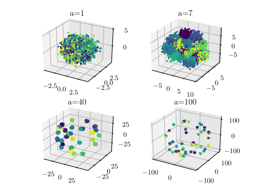
Fig. 1: Visualization of GM data geometries using (10). As $a$ increases the inter-component separability increases.

The signal power $\mathcal{E}\{\|(\mathbf{t}-\mathcal{E}(\mathbf{t})\|^{2}\}$ is shown in (LABEL:eq:Signal_power_1) as,

(14)

The noise power is $\mathcal{E}\{\|(\mathbf{n}-\mathcal{E}(\mathbf{n})\|^{2}\}=\sum_{i=1}^{P}\mathcal{E}(n_{i}^{2})=P\frac{b}{P}=b$. The signal-to-noise-ratio (SNR) in dB is,

$$SNR=10\log_{10}\frac{\mathcal{E}\{\|(\mathbf{t}-\mathcal{E}(\mathbf{t})\|^{2}\}}{\mathcal{E}\{\|(\mathbf{n}-\mathcal{E}(\mathbf{n})\|^{2}\}}$$ (15)

$$=10\log_{10}\frac{Q+a^{2}\left(1-\frac{1}{M^{2}}\operatorname{Tr}[\sum_{m=1}^{M}\boldsymbol{\mu}_{m}][\sum_{m=1}^{M}\boldsymbol{\mu}_{m}]^{T}\right)}{b}.$$

For the data generation, we sample $\mathbf{t}$ and $\mathbf{n}$ from the distributions (4), and generate $\mathbf{x}$ using (3). We denote the training set as $\mathcal{D}_{train}=\{(\mathbf{x}^{(j)},\mathbf{t}^{(j)})\}_{j=1}^{J_{train}}$ with $J_{train}$ data-and-target pairs and the test set as $\mathcal{D}_{test}=\{(\mathbf{x}^{(j)},\mathbf{t}^{(j)})\}_{j=1}^{J_{test}}$ with $J_{test}$ data-and-target pairs. The experiments are carried out in Monte-Carlo fashion over many realizations of observation system matrix $\mathbf{H}$ and the results are shown averaged over those realizations. The components of $\mathbf{H}$ are i.i.d Gaussian.

3.2 Experiments

Experiments are performed to understand several aspects of the NNs. We choose four types of NNs: extreme learning machine (ELM) [18], self-size estimating feedforward NN (SSFN) [19], feedforward NN (FFNN) [20], and residual network (ResNet) [21]. The choice of NNs is based on their structures and training complexity.

We choose an ELM with a single hidden layer comprised of 30 hidden nodes. The ELM uses a random weight matrix. Therefore ELM is a simple network to train. The SSFN is a multi-layer network with low training complexity. The SSFN uses a combination of random weights and learned parameters. We used a 20-layer SSFN with 30 hidden nodes per layer. Then we evaluate a FFNN with 6 hidden layers. The number of nodes are 64, 128, 256, 256, 128, 64 for the six layers, respectively. FFNN is trained using standard backpropagation. Finally we use ResNet-34 to have a deep NN that has capability to avoid the vanishing gradient problem [21]. The ResNet-34 is a 34 layered architecture with a combination of convolutional layers, max-pooling, batch normalization and skip connections. We adapted it from Keras ResNet-50 structure with one change - use of 1-D convolution instead of 2-D convolution because of our data type. The number of trainable parameters are approximately 0.3K, 6K, 240K, and 500K for ELM, SSFN, FFNN, and ResNet-34, respectively. All the experiments were performed with a train:test split of $70:30$ using $10$ Monte Carlo simulations.

Our first three experiments are conducted in matched training and testing statistics scenario, which means we first fix the parameters of distributions to define the signal statistics and then generate $\mathcal{D}_{train}$ and $\mathcal{D}_{test}$. In our first experiment, we study the effect of training dataset size $\mathcal{D}_{train}$. The estimation performance versus size of training dataset is shown in Fig. 2. The experiment shows that performances of all the four NNs saturate as the training data size increases. Therefore the popular idea that more and more training data improves the learning capacity of NNs is questionable. Based on the saturation trend, we decide to perform rest of the experiments using 3000 total data.

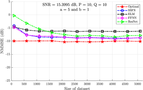
Fig. 2: Estimation performance study for visualizing the effect of training data amount.

The second experiment is designed to study how the data geometry affects the estimation performance. The choice $b=50$ translates to a fixed noise power. The SNR is varied by varying $a$. We show estimation performance versus SNR in Fig. 3. The results show that all NNs show bad performance when SNR is low. As the SNR improves, performance of all four NNs improves, but FFNN and ResNet outperform others. The performance of ResNet saturates at high SNR.

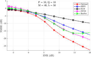
Fig. 3: Estimation performance study for visualizing role of data geometry and the resulting signal power.

The third experiment studies sampling requirements. This is represented by the observation vector dimension $P$ for a fixed target signal dimension $Q$. Note that $P<Q$ is a under-determined sampling system, and $P\geq Q$ is an over-determined system. The NMSE versus $P$ for $Q=10$ is shown in Fig. 4. The results show performance improvement as $P$ increases and then a saturation trend.

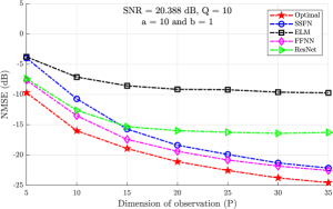
Fig. 4: Estimation performance study for visualizing the role of sampling.

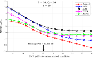
Fig. 5: Estimation performance study for mismatched training and testing conditions. The training SNR is 10.396 dB.

All the previous experiments used matched training and test statistics. We now consider mismatched training and test statistics for our last experiment. A mismatched scenario is relevant in reality. In this case, different parameter settings are used to generate $\mathcal{D}_{train}$ and $\mathcal{D}_{test}$. The training SNR is chosen as 10.396 dB. We vary $b$ to change test SNR keeping all other parameters same as the training condition, and then we create $\mathcal{D}_{test}$ for a choice of $b$. The performances for different test SNRs are shown in Fig. 5. The results show that the NNs behave in a similar manner according to Fig. 3 in the region closer to matched training and test statistics. An interesting observation is that all the four NNs show a saturation trend when test SNR increases. This result shows that training based estimators (NNs) do not generalize under different testing conditions, even when test SNR improves.

A natural question is why ResNet-34 does not show the best performance among the competing NNs, given ResNet is known to provide a high quality performance for image classification. Our understanding is that the GMM based data that we generated, does not have similar spatial correlations like images. The convolutional filters, max-pooling and skip connections of ResNet are more suitable for image signals. Therefore it is important to understand the type and statisitical conditions of data for appropriate use and design of NNs.

Code is available here: https://github.com/s-a-n-d-y/ExAI.

4 conclusions

We show that it is possible to compare between NNs using generated data in a controllable experimental setup, and have an understanding of achievable performance by comparing with the MMSE bound. A large gap between performance and MMSE bound motivates effort to design efficient NNs. We conclude with an understanding that an efficient NN for a particular data type or statistical condition may not show good performance for a different data type or statistical condition.

References

- [1] W. Samek, Grégoire Montavon, A. Vedaldi, L. Hansen, and K. Müller, “Explainable ai: Interpreting, explaining and visualizing deep learning,” Explainable AI: Interpreting, Explaining and Visualizing Deep Learning, 2019.
- [2] Laura Rieger and Lars Kai Hansen, “Aggregating explainability methods for neural networks stabilizes explanations,” CoRR, vol. abs/1903.00519, 2019.
- [3] Zachary C Lipton, “The mythos of model interpretability,” Queue, vol. 16, no. 3, pp. 31–57, 2018.
- [4] Marco Tulio Ribeiro, Sameer Singh, and Carlos Guestrin, “”why should i trust you?”: Explaining the predictions of any classifier,” Proceedings of the 22nd ACM SIGKDD International Conference on Knowledge Discovery and Data Mining, p. 1135–1144, 2016.
- [5] Vishal Monga, Yuelong Li, and Yonina C Eldar, “Algorithm unrolling: Interpretable, efficient deep learning for signal and image processing,” Accepted for IEEE Signal Processing Magazine, 2020.
- [6] Marina Danilevsky, Kun Qian, Ranit Aharonov, Yannis Katsis, Ban Kawas, and Prithviraj Sen, “A survey of the state of explainable ai for natural language processing,” ArXiv e-prints, 2020.
- [7] Jason Yosinski, Jeff Clune, Anh Nguyen, Thomas Fuchs, and Hod Lipson, “Understanding neural networks through deep visualization,” in Deep Learning Workshop, International Conference on Machine Learning (ICML), 2015.
- [8] Raghavendra Kotikalapudi and contributors, “keras-vis,” Available online at https://github.com/raghakot/keras-vis, 2017.
- [9] Santiago A. Cadena, Marissa A. Weis, Leon A. Gatys, Matthias Bethge, and Alexander S. Ecker, “Diverse feature visualizations reveal invariances in early layers of deep neural networks,” in Computer Vision – ECCV 2018, Cham, 2018, pp. 225–240, Springer International Publishing.
- [10] Bolei Zhou, Aditya Khosla, Agata Lapedriza, Aude Oliva, and Antonio Torralba, “Learning deep features for discriminative localization,” in Computer Vision and Pattern Recognition, 2016.
- [11] Jorg Wagner, Jan Mathias Kohler, Tobias Gindele, Leon Hetzel, Jakob Thaddaus Wiedemer, and Sven Behnke, “Interpretable and fine-grained visual explanations for convolutional neural networks,” in Proceedings of the IEEE Conference on Computer Vision and Pattern Recognition, 2019, pp. 9097–9107.
- [12] Ismael Lemhadri, Feng Ruan, and Robert Tibshirani, “A neural network with feature sparsity.,” CoRR, 2019.
- [13] Seyed-Mohsen Moosavi-Dezfooli, Alhussein Fawzi, and Pascal Frossard, “Deepfool: a simple and accurate method to fool deep neural networks,” in Proceedings of the IEEE conference on computer vision and pattern recognition, 2016, pp. 2574–2582.
- [14] I. Kobyzev, S. Prince, and M. Brubaker, “Normalizing flows: An introduction and review of current methods,” IEEE Transactions on Pattern Analysis and Machine Intelligence, pp. 1–1, 2020.
- [15] Ian Goodfellow, Yoshua Bengio, and Aaron Courville, “Deep learning,” pp. 65–66. MIT Press, 2016.
- [16] Achintya Kundu, Saikat Chatterjee, A. Sreenivasa Murthy, and T. V. Sreenivas, “GMM based bayesian approach to speech enhancement in signal /transform domain,” ICASSP, IEEE International Conference on Acoustics, Speech and Signal Processing - Proceedings, pp. 4893–4896, 2008.
- [17] Steven M. Kay, Fundamentals of Statistical Signal Processing: Estimation Theory, Prentice-Hall, Inc., USA, 1993.
- [18] Guang-Bin Huang, Qin-Yu Zhu, and Chee-Kheong Siew, “Extreme learning machine: Theory and applications,” Neurocomputing, vol. 70, no. 1, pp. 489 – 501, 2006.
- [19] Saikat Chatterjee, Alireza M. Javid, Mostafa Sadeghi, Shumpei Kikuta, Dong Liu, Partha P. Mitra, and Mikael Skoglund, “SSFN – Self Size-estimating Feed-forward Network with Low Complexity, Limited Need for Human Intervention, and Consistent Behaviour across Trials,” ArXiv e-prints, 2019.
- [20] Kurt Hornik, Maxwell Stinchcombe, and Halbert White, “Multilayer feedforward networks are universal approximators,” Neural Networks, vol. 2, no. 5, pp. 359 – 366, 1989.
- [21] Kaiming He, Xiangyu Zhang, Shaoqing Ren, and Jian Sun, “Deep residual learning for image recognition,” in Proceedings of the IEEE conference on computer vision and pattern recognition, 2016, pp. 770–778.