Semi-blind Channel Estimation and Data Detection for Multi-cell Massive MIMO Systems on Time-Varying Channels

Abstract

We study the problem of semi-blind channel estimation and symbol detection in the uplink of multi-cell massive MIMO systems with spatially correlated time-varying channels. An algorithm based on expectation propagation (EP) is developed to iteratively approximate the joint a posteriori distribution of the unknown channel matrix and the transmitted data symbols with a distribution from an exponential family. This distribution is then used for direct estimation of the channel matrix and detection of data symbols. A modified version of the popular Kalman filtering algorithm referred to as KF-M emerges from our EP derivation and it is used to initialize the EP-based algorithm. Performance of the Kalman smoothing algorithm followed by KF-M is also examined. Simulation results demonstrate that channel estimation error and the symbol error rate (SER) of the semi-blind KF-M, KS-M, and EP-based algorithms improve with the increase in the number of base station antennas and the length of the data symbols in the transmitted frame. It is shown that the EP-based algorithm significantly outperforms KF-M and KS-M algorithms in channel estimation and symbol detection. Finally, our results show that when applied to time-varying channels, these algorithms outperform the algorithms that are developed for block-fading channel models.

I Introduction

In wireless communication, coherent demodulation of transmitted symbols requires accurate knowledge of channel state information (CSI). Traditionally, pilot sequences are transmitted to aid in channel estimation. Since the number of transmit antennas determines the length of the orthogonal pilot sequences, for massive MIMO systems employing a large number of antennas at the base station (BS), pilot-based channel estimation in the downlink is very challenging. Due to the increased length of pilot sequences, the time required for pilot transmission increases resulting in low spectral efficiency. In addition, the time required for data and pilot transmission may exceed the coherence time of the channel.

In time division duplexing (TDD), CSI can be estimated in the uplink from pilot transmissions. For users employing a single antenna, the length of the pilot sequence only needs to scale with the number of users in the cell which is typically much smaller than the number of BS antennas. Invoking the channel reciprocity property, the uplink CSI matrix is transposed to obtain the downlink CSI which can then be used for precoding in the downlink. However, even in this case, due to the limited number of orthogonal pilot sequences, pilots must be shared among the users in the neighboring cells resulting in the so-called pilot contamination problem [1], which diminishes the accuracy of CSI estimation.

To overcome the effects of pilot contamination, several blind channel estimation schemes have been proposed in recent years [2, 3, 4, 5]. In [2] the expectation propagation (EP) algorithm [6] is developed for blind channel estimation and symbol detection in multi-cell massive MIMO systems. Bilinear generalized approximate message passing (BiG-AMP) algorithm is another approach proposed in [3] for sparse massive MIMO channels. Channel sparsity is exploited in a number of other studies including [4, 5, 7]. In particular [5] studies the effect of one-bit ADCs in the receiver.

Blind channel estimation methods suffer from inherent phase ambiguities in the demodulated symbols, requiring a pilot symbol and user label in order to resolve these ambiguities [3]. In contrast, adding a few additional training symbols in a semi-blind approach significantly improves the channel estimation accuracy compared to the blind methods (see Fig. $1$ in [8, 9]). A semi-blind channel estimation method based on the expectation maximization algorithm is proposed and analyzed in [10]. A semi-blind pilot decontamination scheme is proposed for a multi-cell massive MIMO system in [11] where the information sequence of the target cell is first estimated and used as a pilot sequence in a least square method for CSI estimation. In [12] the authors present a semi-blind joint channel estimation and data detection method based on the regularized alternating least-square (R-ALS) method. Other semi-blind algorithms for massive MIMO channels are proposed in [13, 9] where the pilots sent in the beginning portion of the frames are used for their initialization. For sparse massive MIMO channels, a message passing semi-blind channel estimation algorithm is proposed in [14].

In the semi-blind algorithms described above, the massive MIMO channel is assumed to be spatially uncorrelated, as well as static during the transmission time of a frame. Due to their large number of antennas, the BS’s in massive MIMO systems have fine angular resolutions making some spatial directions more probable than others [15, 16, 17]. This results in spatial correlation in the channel vector of a user to the BS which needs to be included in the channel model. Secondly, while the assumption of static channel (the so-called block-fading) model is valid for stationary or low-mobility users, it breaks down for high-mobility users. In addition to delay spread due to multipath effects, mobile fading channels are subject to time variations due to Doppler spread. For block-fading channels CSI estimation is only required at the start of each frame. However, for time-varying channels, the CSI estimates need to be updated instantaneously throughout the frame. Compared to the rich literature available on block-fading channel estimation in massive MIMO systems, few studies are available for the estimation of the time-varying channels. For a time-varying massive MIMO channel, the data rates achievable by the linear MMSE channel estimator is studied in [18, 19, 20, 21]. The time evolution of the channel taps is modeled by a first-order autoregressive (AR) process with the temporal correlation properties corresponding to the Jakes’ model [22]. Kalman filter is used to estimate the time-varying sparse massive MIMO channel in [23] and the time-varying non-sparse massive MIMO channel in [24, 25].

In this paper, we consider semi-blind joint channel estimation and data detection in multi-cell massive MIMO systems for a spatially correlated time-varying channel. To our knowledge, this problem has not been studied for massive MIMO systems. The contributions made in this paper are summarized as follow:

• We consider a multi-user multi-cell massive MIMO system. The uplink channel from each user to BS is assumed to be spatially correlated and time-varying. The channel vector from a user to the BS is modeled as a complex circularly-symmetric Gaussian vector with a given (known) correlation matrix [17]. The temporal correlation of the channel is modeled by a first-order AR process, [18, 19, 21] with correlation properties corresponding to the Jakes’ model [22]. A semi-blind method is developed for joint channel estimation and data detection where it is assumed that the users transmit a few pilot symbols (on the order of the number of users) at the beginning of each frame. These symbols are used for an initial estimation of the channel and to overcome the inherent ambiguity of non-coherent detectors. The proposed method is based on the expectation propagation (EP) algorithm and iteratively approximates the joint a posterior distribution of the channel matrix and the transmitted data symbols with a distribution from an exponential family. This distribution is then used for direct estimation of the channel matrix and detection of the data symbols.

• Simulation results are presented to demonstrate the performance of the proposed EP-based algorithm (EP) in terms of channel estimation and symbol error rate (SER).

  A modified version of the popular Kalman filtering (KF) algorithm referred to as KF-M is also proposed. KF-M emerges from our EP derivation and is used to initialize the EP-based algorithm. The backward recursion equations of Kalman smoother are also a part of our EP derivations. Therefore, the performance of KF-M as well as the Kalman smoothing algorithm followed by a single pass of KF-M is also presented here for comparison and is denoted as KS-M. To benchmark the performance of semi-blind KF-M, KS-M, and EP, we also present the performance of the Kalman filter and smoother in a pure training mode (TM) when the entire frame is composed of known pilot symbols and only channel estimation is performed. These two cases, are referred to as KF-TM and KS-TM. In channel estimation, KF-TM provides a lower bound for KF-M, and KS-TM provides a lower bound for KS-M, and EP. Finally, we also plot the SER performance of the MMSE estimator with known CSI (denoted PCSI) for comparison with SER performance of the proposed algorithms.

• To our knowledge the problem under consideration here has not been previously investigated. As such, unfortunately we cannot compare our results with those in published literature. However, to verify that algorithms developed under the assumption of a block-fading channel are not suitable for a time-varying channel model, we compare our results with those from [10] and [12]. The comparison shows that for time-varying channels, the proposed method significantly outperforms the methods in [10] and [12].

The rest of this paper is organized as follows. Section II describes the system model of a time-varying multicell massive MIMO system. The semi-blind EP algorithm for this system is derived in section III. Simulation results are discussed in section IV and section V concludes this work.

Notations: Throughout this paper, small letters $(x)$ are used for scalars, bold small letters $(\mathbf{x})$ for vectors, and bold capital letters $(\mathbf{X})$ for matrices. $\mathbb{R}$ and $\mathbb{C}$ represent the set of real and complex numbers, respectively. The superscripts $(.)^{T}$, $(.)^{H}$, $(.)^{*}$, and $(.)^{-1}$ represent transpose, Hermitian transpose, complex conjugate, and matrix inverse, respectively. Also, $\otimes$ denotes the matrix Kronecker product. For a pdf $p(.)$, $\mathbb{E}_{p}$ denotes the expectation operator with respect to $p(.)$. $\mathbf{I}_{N}$ denotes the $N\times N$ identity matrix. Finally, $\operatorname{vec}(\mathbf{X})$ and $||\mathbf{x}||$ denote the vectorization of the matrix $\mathbf{X}$ and the $\ell^{2}$ norm of the vector $\mathbf{x}$, respectively.

II System Model

We consider a multi-user MIMO network made up of $L$ cells each with its own BS and with $K$ users located inside every cell. Every BS in a cell has $M$ antennas and each user has a single-antenna transceiver. At time $t$, the channel gain between the $m$-th antenna of the $l$-th BS and the $k$-th user present in the $i$-th cell is represented by ${h}_{limk}(t)$. Each channel gain ${h}_{limk}(t)$ can be written as

$${h}_{limk}(t)={g}_{limk}(t)\sqrt{\beta_{lik}},$$ (1)

where, ${g}_{limk}(t)$ models the fast-fading channel between the $k$-th user in cell $i$ and the $m$-th antenna of BS $l$, and $\beta_{lik}$ models the large-scale fading incurred by the geometric attenuation and shadowing effects. We assume that $\beta_{lik}$ is a known constant which is independent of the antenna index $m$.

The fast-fading channel ${g}_{limk}(t)$ is considered to be a wide-sense stationary complex Gaussian process with zero mean and unit power. Using the Jakes’ model [22], the time autocorrelation of ${g}_{limk}(t)$ is given by

$$R^{g}_{limk}\left(\Delta t\right) =\mathbb{E}\left[{g}_{limk}(t){g}^{*}_{limk}(t+\Delta t)\right]$$

$$=J_{0}\left(2\pi f^{d}_{limk}|\Delta t|\right),$$ (2)

in which, $J_{0}(.)$ is the zero-order Bessel function of first kind and $f^{d}_{limk}$ represents the normalized maximum Doppler shift corresponding to the channel between the $m$-th antenna of cell $l$ and the $k$-th user in cell $i$. The time autocorrelation function of $h_{limk}(t)$ can be obtained as

$$R^{h}_{limk}\left(\Delta t\right) =\mathbb{E}\left[{h}_{limk}(t){h}^{*}_{limk}(t+\Delta t)\right]$$

$$=\beta_{lik}\mathbb{E}\left[{g}_{limk}(t){g}^{*}_{limk}(t+\Delta t)\right]$$

$$=\beta_{lik}J_{0}\left(2\pi f^{d}_{limk}|\Delta t|\right),$$ (3)

Let ${\mathbf{g}_{lik}(t)}\triangleq[{g}_{li1k}(t),{g}_{li2k}(t),\ldots,{g}_{liMk}(t)]^{T}$ represent the $M\times 1$ fast-fading channel vector from the $k$-th user in cell $i$ to the $l$-th BS antenna array. We assume that the elements in $\mathbf{g}_{lik}(t)$ are correlated with the correlation matrix $\mathbf{R}_{lik}\triangleq\mathbb{E}[\mathbf{g}_{lik}(t)\mathbf{g}^{H}_{lik}(t)]$ [26, 27]. Let ${\mathbf{G}}_{li}(t)\triangleq[{\mathbf{g}}_{li1}(t),\ldots,{\mathbf{g}}_{liK}(t)]$. The overall channel gain between the $l$-th BS and the users in cell $i$ is given by

$$\mathbf{H}_{li}(t)\triangleq{\mathbf{G}}_{li}(t)\mathbf{D}_{li}^{\frac{1}{2}},$$ (4)

where $\mathbf{D}_{li}\triangleq\operatorname{diag}\{\beta_{li1},\beta_{li2},\ldots,\beta_{liK}\}$. It is assumed that the users’ channels to the BS are uncorrelated. In particular this implies that $\mathbb{E}[{\mathbf{G}}_{li}(t){\mathbf{G}}_{lj}^{H}(t)]=\sum^{K}_{k=1}\mathbb{E}[\mathbf{g}_{lik}(t)\mathbf{g}^{H}_{ljk}(t)]=\sum^{K}_{k=1}\mathbf{R}_{lik}\delta_{ij}$, and as a result,

$$\mathbb{E}[\mathbf{H}_{li}(t)\mathbf{H}_{lj}^{H}(t)] =\mathbb{E}[\mathbf{G}_{li}(t)\mathbf{D}_{li}\mathbf{G}_{li}^{H}(t)]\delta_{ij},$$

$$=\sum_{k=1}^{K}\beta_{lik}\mathbf{R}_{lik}\delta_{ij},$$ (5)

The signal vector received at BS $l$ at time $t$ is given by

$$\mathbf{y}_{l}(t) =\sum_{i=1}^{L}\mathbf{H}_{li}(t)\mathbf{s}_{i}(t)+\mathbf{w}^{\prime}_{l}(t)$$

$$=\underbrace{\mathbf{H}_{ll}(t)\mathbf{s}_{l}(t)}_{\text{desired signal}}+\underbrace{\sum_{\stackrel{{\scriptstyle i=1}}{{i\neq l}}}^{L}\mathbf{H}_{li}(t)\mathbf{s}_{i}(t)}_{\text{interference}}+\underbrace{\mathbf{w}^{\prime}_{l}(t)}_{\text{noise}},$$ (6)

where $\mathbf{s}_{i}(t)=[s_{i1}(t),s_{i2}(t),\ldots,s_{iK}(t)]^{T}$ represents the transmitted symbols by all the users in the $i$-th cell. We assume that the symbols $s_{ij}(t)$ belong to an $\mathcal{M}$-ary modulation constellation, denoted by $\mathcal{A}_{\mathcal{M}}$, and have zero mean with average energy $E_{s}$. We also assume that $\mathbb{E}[\mathbf{s}_{i}(t)\mathbf{s}_{j}(t)^{H}]=E_{s}\delta_{ij}\mathbf{I}_{K}$, i.e., the symbols $s_{ij}(t)$ are independently selected from $\mathcal{A}_{\mathcal{M}}$. The noise term at the $l$-th BS is modeled with a circularly symmetric complex Gaussian distribution, i.e., $\mathbf{w}^{\prime}_{l}(t)\sim\mathcal{CN}(\mathbf{w}^{\prime}_{l}|\mathbf{0},\mathbf{I}_{M})$.

Let $\mathbf{w}_{l}(t)\triangleq\sum_{\stackrel{{\scriptstyle i=1}}{{i\neq l}}}^{L}\mathbf{H}_{li}(t)\mathbf{s}_{i}(t)+\mathbf{w}^{\prime}_{l}(t)$ denote the overall disturbance at the $l$-th BS. Thus, (6) can be written as $\mathbf{y}_{l}(t)=\mathbf{H}_{ll}(t)\mathbf{s}_{l}(t)+\mathbf{w}_{l}(t)$ where $\mathbf{w}_{l}(t)$ has zero mean and correlation matrix

$$\mathbf{R}_{w}\triangleq\mathbb{E}[\mathbf{w}_{l}(t)\big{(}\mathbf{w}_{l}(t)\big{)}^{H}]=E_{s}\sum_{\stackrel{{\scriptstyle i=1}}{{i\neq l}}}^{L}\sum_{k=1}^{K}\beta_{lik}\mathbf{R}_{lik}+\mathbf{I}_{M},$$ (7)

Assuming that $KL$ is large and using the central limit theorem we consider $\mathbf{w}_{l}(t)$ as a circularly symmetric complex-valued Gaussian vector, i.e., $\mathbf{w}_{l}(t)\sim\mathcal{CN}\left(\mathbf{w}_{l}|\mathbf{0},\mathbf{R}_{w}\right)$.

To keep the notations uncluttered, in the following we drop the subscript $l$ from the signal model and write the received vector at time $t$ at the $l$-th BS as

$$\mathbf{y}_{t}=\mathbf{H}_{t}\mathbf{s}_{t}+\mathbf{w}_{t},$$ (8)

where $\mathbf{H}_{t}$ is the overall channel gain matrix, $\mathbf{s}_{t}\in\mathcal{A}_{\mathcal{M}}^{K}$ represents the transmitted symbols by the $K$ users, and $\mathbf{w}_{t}$ is the zero mean complex Gaussian distributed disturbance with covariance matrix given by (7).

By applying the vectorization property as in [2], (8) can also be written as

$$\mathbf{y}_{t}=\mathbf{S}_{t}\mathbf{h}_{t}+\mathbf{w}_{t},$$ (9)

where we define $\mathbf{S}_{t}=\mathbf{s}_{t}^{T}\otimes\mathbf{I}_{M}$ and $\mathbf{h}_{t}=\operatorname{vec}(\mathbf{H}_{t})$.

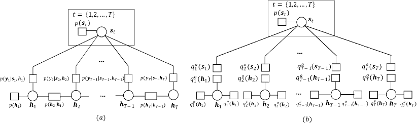
Figure 1: Factor graph illustrations of $(a)$ True posterior distribution in (11), and $(b)$ Approximated posterior distribution in (18). Small rectangles represent factor nodes and circles represent variable nodes. A plate (big rectangle) notation is used to represent a repetition of variables in the subgraph.

An autoregressive (AR) process has been extensively used to model the time evolution of the channel matrix [28, 29, 30, 31]. Since any higher-order AR model can be written as a first-order model in matrix state-space form [30, 21], in this paper we use a first-order AR model (AR(1)) for the time-varying vector channel given by

$$\mathbf{h}_{t}=\mathbf{A}\mathbf{h}_{t-1}+\mathbf{v}_{t},$$ (10)

where $\mathbf{A}$ is a diagonal matrix with the elements on the diagonal denoted by $[\mathbf{A}]_{n,n}=a_{n}$, for $n=1,2,\dots,MK$. The variable $a_{n}$ is the AR(1) coefficient corresponding to the $n$-th channel between a user and a BS antenna in the cell. We let $a_{n}=J_{0}(2\pi f^{d}_{n})$ in which $f^{d}_{n}$ is the normalized maximum Doppler shift for channel $n$. The innovation process $\{\mathbf{v}_{t}\}$ is an iid circularly symmetric complex Gaussian process with ${\mathbf{v}}_{t}\sim\mathcal{CN}(\mathbf{0},\mathbf{Q})$. To include the spatial correlation of the channel vector, we set $\mathbf{Q}=\mathbf{R}^{1/2}_{h}\mathbf{Q}_{v}\mathbf{R}^{1/2}_{h}$ in which, given the independence of users’ channels, $\mathbf{R}_{h}\triangleq\mathbb{E}[\mathbf{h}_{t}\mathbf{h}^{H}_{t}]=\operatorname{diag}\{\beta_{1}\mathbf{R}_{1},\beta_{2}\mathbf{R}_{2},\ldots,\beta_{K}\mathbf{R}_{K}\}$ is a block diagonal matrix. The matrix $\mathbf{Q}_{v}$ is diagonal with elements on the diagonal given by $[\mathbf{Q}_{v}]_{n,n}=\sigma^{2}_{n}$, for $n=1,2,\dots,MK$. To match the autocorrelation function in (II) such that the average power of the channel coefficient in (1) is equal to the large-scale fading coefficient, we set $\sigma^{2}_{n}=(1-a^{2}_{n})$.

Consider a transmitted frame of length $T$ which is comprised of $T_{p}$ pilot symbols in the beginning followed by $T_{d}=T-T_{p}$ unknown data symbols denoted as $\bm{\mathcal{S}}\triangleq\left(\bm{\mathcal{S}}_{p},\bm{\mathcal{S}}_{d}\right)$ where we define $\bm{\mathcal{S}}_{p}=\left(\mathbf{s}_{1},\mathbf{s}_{2},\ldots,\mathbf{s}_{T_{p}}\right)$ and $\bm{\mathcal{S}}_{d}=\left(\mathbf{s}_{T_{p}+1},\ldots,\mathbf{s}_{T}\right)$. The corresponding received vectors are given by $\bm{\mathcal{Y}}\triangleq\left(\bm{\mathcal{Y}}_{p},\bm{\mathcal{Y}}_{d}\right)$, $\bm{\mathcal{Y}}_{p}=(\mathbf{y}_{1},\mathbf{y}_{2},\ldots,\mathbf{y}_{T_{p}})$ and $\bm{\mathcal{Y}}_{d}=(\mathbf{y}_{T_{p}+1},\ldots,\mathbf{y}_{T})$. Similarly, the channel vector is denoted by $\bm{\mathcal{H}}\triangleq\left(\bm{\mathcal{H}}_{p},\bm{\mathcal{H}}_{d}\right)=(\mathbf{h}_{1},\mathbf{h}_{2},\ldots,\mathbf{h}_{T_{p}},\mathbf{h}_{T_{p}+1},\ldots,\mathbf{h}_{T})$. We are interested in a detector where, having received $\bm{\mathcal{Y}}$, the unknown channel vectors in $\bm{\mathcal{H}}$ and the unknown transmitted symbols in $\bm{\mathcal{S}}_{d}$ are jointly estimated. The posterior joint distribution of $\bm{\mathcal{S}}$ and $\bm{\mathcal{H}}$ is given by

$$p(\bm{\mathcal{S}},\bm{\mathcal{H}}|\bm{\mathcal{Y}}) \propto p(\bm{\mathcal{S}}_{d},\bm{\mathcal{H}})p(\bm{\mathcal{Y}}_{p}|\bm{\mathcal{S}}_{p},\bm{\mathcal{H}}_{p})p(\bm{\mathcal{Y}}_{d}|\bm{\mathcal{S}}_{d},\bm{\mathcal{H}}_{d})$$

$$=\Big{[}\prod_{t=T_{p}+1}^{T}p(\mathbf{s}_{t})\Big{]}\Big{[}\prod_{t=1}^{T}p(\mathbf{h}_{t}|\mathbf{h}_{t-1})p(\mathbf{y}_{t}|\mathbf{s}_{t},\mathbf{h}_{t})\Big{]}$$

$$=\prod_{t=1}^{T}p(\mathbf{s}_{t})p(\mathbf{h}_{t}|\mathbf{h}_{t-1})p(\mathbf{y}_{t}|\mathbf{s}_{t},\mathbf{h}_{t}),$$ (11)

in which $p(\mathbf{s}_{t})$ is the probability mass function (pmf) of the transmitted vector $\mathbf{s}_{t}$ and by convention we set $p(\mathbf{s}_{t})=1$ for $t=1,\ldots,T_{p}$ and $p(\mathbf{h}_{1})=p(\mathbf{h}_{1}|\mathbf{h}_{0})$. From (9) we have

$$p(\mathbf{y}_{t}|\mathbf{s}_{t},\mathbf{h}_{t})=\mathcal{CN}(\mathbf{y}_{t}|\mathbf{S}_{t}\mathbf{h}_{t},\mathbf{R}_{w}),$$ (12)

The optimum receiver implements the maximum a posteriori rule according to (13), i.e.,

$$(\bm{\mathcal{S}}_{d},\bm{\mathcal{H}})^{*}=\operatorname*{arg\,max}_{\bm{\mathcal{S}}_{d}\in\mathcal{A}_{\mathcal{M}}^{KT_{d}},\bm{\mathcal{H}}\in\mathbb{C}^{M\times T}}p(\bm{\mathcal{S}},\bm{\mathcal{H}}|\bm{\mathcal{Y}}),$$ (13)

Due to the complexity of (13), finding the optimum solution is generally very difficult and requires multidimensional integration. The proposed EP algorithm in the next section exploits the multiplicative nature of (11) to find a simpler approximation for the conditional joint distribution of $(\bm{\mathcal{S}},\bm{\mathcal{H}})$ such that the marginals can be calculated with much less effort.

III Semi-blind EP formulation

In this section we develop the EP algorithm for noncoherent semi-blind detection in massive MIMO systems for fast fading channel. For a review of the EP algorithm we refer to [32, 33]. Let $\mathcal{F}$ denote a family of exponential distributions. Similar to [31] we exploit the factorized structure of (11) to approximate the posterior distribution $p(\bm{\mathcal{S}},\bm{\mathcal{H}}|\bm{\mathcal{Y}})$ with the following distributions from $\mathcal{F}$.

$$p(\bm{\mathcal{S}},\bm{\mathcal{H}}|\bm{\mathcal{Y}})\approx q(\bm{\mathcal{S}},\bm{\mathcal{H}})=\prod_{t=1}^{T}q_{t}(\mathbf{s}_{t},\mathbf{h}_{t})=\prod_{t=1}^{T}q_{t}(\mathbf{s}_{t})q_{t}(\mathbf{h}_{t}),$$ (14)

where $q_{t}(\mathbf{s}_{t},\mathbf{h}_{t})=q_{t}(\mathbf{s}_{t})q_{t}(\mathbf{h}_{t})$ $\in\mathcal{F}$. Examining (11) and following [31], we use the following product form for ${q}(\bm{\mathcal{S}},\bm{\mathcal{H}})$:

$$q(\bm{\mathcal{S}},\bm{\mathcal{H}}) \propto p(\mathbf{s}_{1})p(\mathbf{h}_{1})q_{1}^{O}(\mathbf{s}_{1},\mathbf{h}_{1})\times$$

$$\prod_{t=2}^{T}p(\mathbf{s}_{t})q_{t}^{FR}(\mathbf{h}_{t-1},\mathbf{h}_{t})q_{t}^{O}(\mathbf{s}_{t},\mathbf{h}_{t}),$$ (15)

where, comparing (15) and (11), we have $q_{t}^{FR}(\mathbf{h}_{t-1},\mathbf{h}_{t})$ to approximate $p(\mathbf{h}_{t}|\mathbf{h}_{t-1})$ and $q_{t}^{O}(\mathbf{s}_{t},\mathbf{h}_{t})$ to approximate $p(\mathbf{y}_{t}|\mathbf{s}_{t},\mathbf{h}_{t})$. Finally, to write (15) in a completely factorized form as in (14) we let

$$q_{t}^{O}(\mathbf{s}_{t},\mathbf{h}_{t})=q_{t}^{O}(\mathbf{s}_{t})q_{t}^{O}(\mathbf{h}_{t}),$$ (16)

and

$$q_{t}^{FR}(\mathbf{h}_{t-1},\mathbf{h}_{t})=q_{t}^{R}(\mathbf{h}_{t-1})q_{t}^{F}(\mathbf{h}_{t}),$$ (17)

Now inserting (16) and (17) into (15), and letting $q_{1}^{F}(\mathbf{h}_{1})$ to approximate $p(\mathbf{h}_{1})$ and $q_{T}^{R}(\mathbf{h}_{T})=1$, we can write

$$q(\bm{\mathcal{S}},\bm{\mathcal{H}})\propto\Big{[}\prod_{t=1}^{T}p(\mathbf{s}_{t})q_{t}^{O}(\mathbf{s}_{t})\Big{]}\Big{[}\prod_{t=1}^{T}q_{t}^{F}(\mathbf{h}_{t})q_{t}^{R}(\mathbf{h}_{t})q_{t}^{O}(\mathbf{h}_{t})\Big{]},$$ (18)

From (18) and (14), the approximating posterior distribution $q_{t}(\mathbf{s}_{t},\mathbf{h}_{t})$ is given by

$$q_{t}(\mathbf{s}_{t},\mathbf{h}_{t})\propto p(\mathbf{s}_{t})q_{t}^{R}(\mathbf{h}_{t})q_{t}^{F}(\mathbf{h}_{t})q_{t}^{O}(\mathbf{s}_{t})q_{t}^{O}(\mathbf{h}_{t}),$$ (19)

Note that in (19), from (11) we have $p(\mathbf{s}_{t})=1$ for all $t=1,\ldots,T_{p}$. The true posterior distribution in (11) and the approximate one in (18) are illustrated with factor graphs in Fig. 1. Updating the factors $q^{F}_{t}(.)$, $q^{R}_{t}(.)$, and $q^{O}_{t}(.)$ in (19) result in forward, reverse, and observation messages, respectively, which propagate through the factor graph in Fig. 1 (a) until a good approximation to the true posterior is obtained.

With EP, we update the factors ensuring that they belong to the exponential family $\mathcal{F}$. As a result, their product $q(\bm{\mathcal{S}},\bm{\mathcal{H}})$ also belongs to $\mathcal{F}$ and can be effectively used for maximum a posteriori estimation. To this end, we select the distributions $q_{t}^{O}(\mathbf{h}_{t})$, $q_{t}^{F}(\mathbf{h}_{t})$ and $q_{t}^{R}(\mathbf{h}_{t})$ from the exponential family $\mathcal{F}$ and $q_{t}^{O}(\mathbf{s}_{t})$ to be discrete. Since $p(\mathbf{s}_{t})$ is also discrete, it follows that (19) and (18) are from the exponential family. In the following, we update these factors.

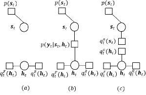
Figure 2: EP steps for updating $q^{O}_{t}(\mathbf{s}_{t},\mathbf{h}_{t})$: $(a)$ Eliminate $q^{O}_{t}(\mathbf{s}_{t})$ and $q^{O}_{t}(\mathbf{h}_{t})$ from the factor graph to find the cavity distribution $q^{\backslash O}_{t}(\mathbf{s}_{t},\mathbf{h}_{t})$ as in (20), $(b)$ Use $p(\mathbf{y}_{t}|\mathbf{s}_{t},\mathbf{h}_{t})$ factor to define the hybrid posterior distribution $\hat{q}_{t}(\mathbf{s}_{t},\mathbf{h}_{t})$ as in (22), and $(c)$ Project $\hat{q}_{t}(\mathbf{s}_{t},\mathbf{h}_{t})$ onto $\mathcal{F}$ and update $q^{O}_{t}(\mathbf{s}_{t},\mathbf{h}_{t})$ as in (33) and (37).

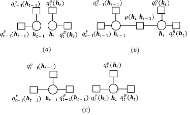
Figure 3: EP steps for updating $q^{R}_{t-1}(\mathbf{h}_{t-1})$ and $q^{F}_{t}(\mathbf{h}_{t})$: $(a)$ Eliminate $q^{R}_{t-1}(\mathbf{h}_{t-1})$ and $q^{F}_{t}(\mathbf{h}_{t})$ from the factor graph to find the cavity distributions $q^{\backslash R}_{t-1}(\mathbf{h}_{t-1})$ and $q^{\backslash F}_{t}(\mathbf{h}_{t})$ as in (38), $(b)$ Use $p(\mathbf{h}_{t}|\mathbf{h}_{t-1})$ factor to define the intermediate posterior distribution $r_{t}(\mathbf{h}_{t-1},\mathbf{h}_{t})$ as in (39), and $(c)$ Project $r_{t}(\mathbf{h}_{t-1},\mathbf{h}_{t})$ onto $\mathcal{F}$ and update $q^{F}_{t}(\mathbf{h}_{t})$, $q^{R}_{t-1}(\mathbf{h}_{t-1})$ as in (45), (46), and (48).

First, we ignore the beginning portion of the frame and compute $q_{t}^{O}(\mathbf{s}_{t})$ and $q_{t}^{O}(\mathbf{h}_{t})$ for the blind part of the frame, i.e., for $t=T_{p}+1,\ldots,T$. As shown in Fig. 2 we define the cavity distribution as

$$q_{t}^{\backslash O}(\mathbf{s}_{t},\mathbf{h}_{t})=\frac{q_{t}(\mathbf{s}_{t},\mathbf{h}_{t})}{q_{t}^{O}(\mathbf{s}_{t})q_{t}^{O}(\mathbf{h}_{t})}=p(\mathbf{s}_{t})q_{t}^{\backslash O}(\mathbf{h}_{t}),$$ (20)

For the exponential family $\mathcal{F}$, we consider the special family of multivariate Gaussian distributions. More specifically, we let $q_{t}^{\backslash O}(\mathbf{h}_{t})\triangleq q_{t}^{F}(\mathbf{h}_{t})q_{t}^{R}(\mathbf{h}_{t})\sim\mathcal{CN}(\mathbf{m}_{t}^{\backslash O},\mathbf{V}_{t}^{\backslash O})$. The discrete distributions $q_{t}^{O}(\mathbf{s}_{t})$ are assumed to be the probability mass functions (pmf) of their corresponding random variables. Denoting $\mathcal{A}_{\mathcal{M}}^{K}\triangleq\{\mathbf{a}_{1},\mathbf{a}_{2},\cdots,\mathbf{a}_{\mathcal{M}^{K}}\}$, the pmf can be defined as

$$q_{t}^{O}(\mathbf{s}_{t})=\left[P(\mathbf{s}_{t}=\mathbf{a}_{1}),\cdots,P(\mathbf{s}_{t}=\mathbf{a}_{\mathcal{M}^{K}})\right]$$ (21)

Next, the hybrid posterior distribution is defined by combining the $t^{th}$ factor in the likelihood function $p(\bm{\mathcal{Y}}|\bm{\mathcal{S}},\bm{\mathcal{H}})$, namely $p(\mathbf{y}_{t}|\mathbf{s}_{t},\mathbf{h}_{t})$, with (20) to get the following intermediate approximate posterior:

$$\hat{q}_{t}(\mathbf{s}_{t},\mathbf{h}_{t})=\frac{p(\mathbf{s}_{t})q_{t}^{\backslash O}(\mathbf{h}_{t})p(\mathbf{y}_{t}|\mathbf{s}_{t},\mathbf{h}_{t})}{Z_{t}},$$ (22)

where $Z_{t}$ is a normalization factor given by

$$Z_{t} =\sum_{\mathbf{s}_{t}\in\mathcal{A}_{\mathcal{M}}^{K}}\int_{\mathbf{h}_{t}}p(\mathbf{s}_{t})q_{t}^{\backslash O}(\mathbf{h}_{t})p(\mathbf{y}_{t}|\mathbf{s}_{t},\mathbf{h}_{t})d\mathbf{h}_{t}$$

$$=\sum_{\mathbf{s}_{t}\in\mathcal{A}_{\mathcal{M}}^{K}}p(\mathbf{s}_{t})\times$$

$$\quad\int_{\mathbf{h}_{t}}\mathcal{CN}(\mathbf{h}_{t}|\mathbf{m}_{t}^{\backslash O},\mathbf{V}_{t}^{\backslash O})\mathcal{CN}(\mathbf{y}_{t}|\mathbf{S}_{t}\mathbf{h}_{t},\mathbf{R}_{w})d\mathbf{h}_{t}$$

$$=\sum_{\mathbf{s}_{t}\in\mathcal{A}_{\mathcal{M}}^{K}}p(\mathbf{s}_{t})\,\mathcal{CN}(\mathbf{y}_{t}|\mathbf{S}_{t}\mathbf{m}_{t}^{\backslash O},\bm{\Sigma}_{t}),$$ (23)

In (23), $\bm{\Sigma}_{t}\triangleq\mathbf{S}_{t}\mathbf{V}_{t}^{\backslash O}\mathbf{S}_{t}^{H}+\mathbf{R}_{w}$. Next we project $\hat{q}_{t}(\mathbf{s}_{t},\mathbf{h}_{t})$ onto the closest distribution (in the sense of Kullback-Leibler divergence) in $\mathcal{F}$ to find $q_{t}(\mathbf{s}_{t},\mathbf{h}_{t})=q_{t}(\mathbf{s}_{t})q_{t}(\mathbf{h}_{t})$:

$$q_{t}(\mathbf{s}_{t},\mathbf{h}_{t}) =\operatorname*{arg\,min}_{q_{t}(\mathbf{s}_{t},\mathbf{h}_{t})\in{\mathcal{F}}}\operatorname{KL}\left(\hat{q}_{t}(\mathbf{s}_{t},\mathbf{h}_{t})\|q_{t}(\mathbf{s}_{t},\mathbf{h}_{t})\right)$$

$$=\operatorname*{arg\,min}_{q_{t}(\mathbf{s}_{t}),q_{t}(\mathbf{h}_{t})\in{\mathcal{F}}}\operatorname{KL}\left(\hat{q}_{t}(\mathbf{s}_{t},\mathbf{h}_{t})\|q_{t}(\mathbf{s}_{t})q(\mathbf{h}_{t})\right),$$ (24)

where $\operatorname{KL}(\cdot\|\cdot)$ denotes the Kullback-Leibler divergence. It is shown in [2] that the above optimization problem can be divided into the following two separate optimizations:

$$q_{t}(\mathbf{h}_{t}) =\operatorname*{arg\,min}_{q_{t}(\mathbf{h}_{t})\in{\mathcal{F}}}\operatorname{KL}\left(\hat{q}_{t}(\mathbf{h}_{t})\|q_{t}(\mathbf{h}_{t})\right),$$ (25)

$$q_{t}(\mathbf{s}_{t}) =\operatorname*{arg\,min}_{q_{t}({\mathbf{s}}_{t})\in{\mathcal{F}}}\operatorname{KL}\left(\hat{q}_{t}({\mathbf{s}}_{t})\|q_{t}({\mathbf{s}}_{t})\right),$$ (26)

where $\hat{q}_{t}(\mathbf{h}_{t})$ and $\hat{q}_{t}({\mathbf{s}}_{t})$ are the marginal distributions of $\mathbf{h}_{t}$ and $\mathbf{s}_{t}$, respectively, derived from their joint distribution $\hat{q}_{t}({\mathbf{s}_{t}},\mathbf{h}_{t})$.

The solution to (25) is obtained from the so-called moment matching property [2]. Since the approximated posterior $q_{t}(\mathbf{h}_{t})\in\mathcal{F}$, we assume $q_{t}(\mathbf{h}_{t})\sim\mathcal{CN}(\mathbf{h}_{t}|\mathbf{m}_{t},\mathbf{V}_{t})$. The moment matching property implies

$$\mathbf{m}_{t} =\mathbb{E}_{\hat{q}_{t}(\mathbf{h}_{t})}[\mathbf{h}_{t}],$$ (27)

$$\mathbf{V}_{t} =\mathbb{E}_{\hat{q}_{t}(\mathbf{h}_{t})}[\mathbf{h}_{t}\mathbf{h}_{t}^{H}]-\mathbf{m}_{t}\mathbf{m}_{t}^{H},$$ (28)

The values of $\mathbf{m}_{t}$ and $\mathbf{V}_{t}$ are given by the following lemma whose proof is omitted here.

Lemma 1.

1. The posterior mean value $\mathbf{m}_{t}$ is given by

   $$\mathbf{m}_{t} =\mathbf{m}_{t}^{\backslash O}+\mathbf{V}_{t}^{\backslash O}\nabla^{H}_{m},$$ (29)

   where

   $$\nabla^{H}_{m} \triangleq\left(\frac{\partial}{\partial\mathbf{m}_{t}^{\backslash O}}\log Z_{t}\right)^{H}$$

   $$=\frac{1}{Z_{t}}\sum_{\mathbf{s}_{t}\in\mathcal{A}_{\mathcal{M}}^{K}}p(\mathbf{s}_{t})\mathcal{CN}(\mathbf{y}_{t}|\mathbf{S}_{t}\mathbf{m}_{t}^{\backslash O},\bm{\Sigma}_{t})\mathbf{S}_{t}^{H}\bm{\Sigma}_{t}^{-1}\bm{\zeta}_{t},$$ (30)

   where $\bm{\zeta}_{t}\triangleq\mathbf{y}_{t}-\mathbf{S}_{t}\mathbf{m}_{t}^{\backslash O}$ and $Z_{t}$ is given in (23).

2. The covariance matrix $\mathbf{V}_{t}$ is given by

   $$\mathbf{V}_{t}=\mathbf{V}_{t}^{\backslash O}-\mathbf{V}_{t}^{\backslash O}\left(\nabla_{m}^{H}\nabla_{m}-\nabla_{V}\right)\mathbf{V}_{t}^{\backslash O}$$ (31)

   where

   $$\nabla_{V} \triangleq\left(\frac{\partial\log Z_{t}}{\partial\mathbf{V}_{t}^{\backslash O}}\right)^{T}$$

   $$=\frac{1}{Z_{t}}\sum_{\mathbf{s}_{t}\in\mathcal{A}_{\mathcal{M}}^{K}}p(\mathbf{s}_{t})\mathcal{CN}\left(\mathbf{y}_{t}|\mathbf{S}_{t}\mathbf{m}_{t}^{\backslash O},\bm{\Sigma}_{t}\right)\times$$

   $$\quad\mathbf{S}_{t}^{H}\left(\bm{\Sigma}_{t}^{-1}\bm{\zeta}_{t}\bm{\zeta}_{t}^{H}\bm{\Sigma}_{t}^{-1}-\bm{\Sigma}_{t}^{-1}\right)\mathbf{S}_{t}$$ (32)

Note that to simplify notation we have dropped the index $t$ from the left side of (1) and (32) here and in the following.

Thus, $q_{t}^{O}(\mathbf{h}_{t})$ can be updated as

$$q_{t}^{O}(\mathbf{h}_{t})=\frac{q_{t}(\mathbf{h}_{t})}{q^{\backslash O}_{t}(\mathbf{h}_{t})}\propto\mathcal{CN}\left(\mathbf{h}_{t}|\mathbf{m}_{t}^{O},\mathbf{V}^{O}_{t}\right).$$ (33)

As discussed in [31], during the iterations of the algorithm, $\mathbf{V}^{O}_{t}$ may become singular. Therefore, to avoid numerical issues we write the mean and covariance as the natural parameters as follows:

$$\bm{\mu}^{O}_{t} =\bm{\Lambda}^{O}_{t}\mathbf{m}^{O}_{t}=\mathbf{V}^{-1}_{t}\mathbf{m}_{t}-\left(\mathbf{V}^{\backslash O}_{t}\right)^{-1}\mathbf{m}^{\backslash O}_{t},$$ (34)

$$\bm{\Lambda}^{O}_{t} =\left(\mathbf{V}^{O}_{t}\right)^{-1}=\mathbf{V}^{-1}_{t}-\left(\mathbf{V}^{\backslash O}_{t}\right)^{-1},$$ (35)

The solution to (26) is to match the pmf of the posterior distribution $q_{t}(\mathbf{s}_{t})$ to the marginal $\hat{q}_{t}(\mathbf{s}_{t})$ which results in

$$q_{t}(\mathbf{s}_{t})=\frac{p(\mathbf{s}_{t})}{Z_{t}}\mathcal{CN}\left(\mathbf{y}_{t}|\mathbf{S}_{t}\mathbf{m}_{t}^{\backslash O},\bm{\Sigma}_{t}\right),$$ (36)

Therefore, $q^{O}_{t}(\mathbf{s}_{t})$ is updated by

$$q^{O}_{t}(\mathbf{s}_{t})=\frac{q_{t}(\mathbf{s}_{t})}{p(\mathbf{s}_{t})}=\frac{1}{Z_{t}}\mathcal{CN}\left(\mathbf{y}_{t}|\mathbf{S}_{t}\mathbf{m}_{t}^{\backslash O},\bm{\Sigma}_{t}\right),$$ (37)

We now consider the beginning portion of the transmitted frame and for $t=1,\ldots,T_{p}$ for which we do not compute $q^{O}_{t}(\mathbf{s}_{t})$ as $\mathbf{s}_{t}$ are the known pilot symbols. To update $q^{O}_{t}(\mathbf{h}_{t})$, given $q^{\backslash O}_{t}(\mathbf{h}_{t})$ the posterior factor $q_{t}(\mathbf{h}_{t})$ can be directly updated from (29) and (31) by using $\nabla^{H}_{m}=\mathbf{S}_{t}^{H}\bm{\Sigma}_{t}^{-1}\bm{\zeta}_{t}$ and $\nabla_{V}=\mathbf{S}_{t}^{H}\left(\bm{\Sigma}_{t}^{-1}\bm{\zeta}_{t}\bm{\zeta}_{t}^{H}\bm{\Sigma}_{t}^{-1}-\bm{\Sigma}_{t}^{-1}\right)\mathbf{S}_{t}$. We should point out that for this part of the frame, the summations in (23), (1), and (32) reduces to a single term corresponding to the known pilot symbol $\mathbf{s}_{t}$. Following this, $q^{O}_{t}(\mathbf{h}_{t})$ can be computed from (34) and (35).

Input: $\bm{\mathcal{Y}}$

Parameters: $\sigma_{w}^{2}$, $\mathbf{A}$, $\mathbf{Q}$, $n$, $\epsilon$, $\mathbf{m}^{\backslash R}_{0}$, $\mathbf{V}^{\backslash R}_{0}$

Output: $\hat{\bm{\mathcal{S}}}_{d}$, $\hat{\bm{\mathcal{H}}}$

/* Initial filtering pass (KF-M run) */

for each $t=\{1,2,\ldots,T\}$ 

       Compute $\mathbf{m}^{F}_{t}$ and $\mathbf{V}^{F}_{t}$ via (47) then set $\mathbf{m}^{\backslash O}_{t}=\mathbf{m}^{F}_{t}$ and $\mathbf{V}^{\backslash O}_{t}=\mathbf{V}^{F}_{t}$.

       if $t>T_{p}$ then

            Maximize $\mathcal{CN}\left(\mathbf{y}_{t}|\mathbf{S}_{t}\mathbf{m}^{\backslash O}_{t},\bm{\Sigma}_{t}\right)$ for $\mathbf{s}_{t}$ to get the maximizer $\hat{\mathbf{s}}_{t}$.

             Use $\hat{\mathbf{s}}_{t}$ in (62) and (63) to compute $\mathbf{m}_{t}$ and $\mathbf{V}_{t}$ from (29) and (31), respectively.

       else

            Use $\mathbf{s}_{t}$ in (62) and (63) to compute $\mathbf{m}_{t}$ and $\mathbf{V}_{t}$ from (29) and (31), respectively.

       end if

      

      Compute $\bm{\mu}^{O}_{t}$ via (34) and $\bm{\Lambda}^{O}_{t}$ via (35).

       Set $\mathbf{m}^{\backslash R}_{t}=\mathbf{m}_{t}$ and $\mathbf{V}^{\backslash R}_{t}=\mathbf{V}_{t}$.

      

end

/* EP run */

for each $i=\{1,2,\ldots,n\}$ 

       if $i>1$ then

             /* filtering pass */

             for each $t=\{1,2,\ldots,T\}$ 

                   Update $\mathbf{m}^{F}_{t}$ and $\mathbf{V}^{F}_{t}$ via (47).

                   For the followed up next smoothing pass, compute $\mathbf{m}^{\backslash R}_{t}$ via (49) and $\mathbf{V}^{\backslash R}_{t}$ via (50).

                  

             end

            

       end if

      /* smoothing pass */

       for each $t=\{T,T-1,\ldots,1\}$ 

             Set $\mathbf{m}_{T}=\mathbf{m}^{\backslash R}_{T}$ and $\mathbf{V}_{T}=\mathbf{V}^{\backslash R}_{T}$.

             if $t<T$ then

                  Update $\mathbf{m}_{t}$ using (57) and $\mathbf{V}_{t}$ using (58).

                  

             end if

            Compute $q^{\backslash O}_{t}(\mathbf{h}_{t})=\frac{q_{t}(\mathbf{h}_{t})}{q^{O}_{t}(\mathbf{h}_{t})}\sim\mathcal{CN}\left(\mathbf{h}_{t}|\mathbf{m}^{\backslash O}_{t},\mathbf{V}^{\backslash O}_{t}\right)$ as follows:

            

$$\mathbf{m}^{\backslash O}_{t} =\mathbf{V}^{\backslash O}_{t}\left(\mathbf{V}^{-1}_{t}\mathbf{m}_{t}-\bm{\mu}^{O}_{t}\right),$$

$$\mathbf{V}^{\backslash O}_{t} =\left(\mathbf{V}^{-1}_{t}-\bm{\Lambda}^{O}_{t}\right)^{-1},$$

if $t>T_{p}$ then

                  Maximize $\mathcal{CN}\left(\mathbf{y}_{t}|\mathbf{S}_{t}\mathbf{m}^{\backslash O}_{t},\bm{\Sigma}_{t}\right)$ for $\mathbf{s}_{t}$ to get the maximizer $\hat{\mathbf{s}}_{t}$.

                  

                  Use $\hat{\mathbf{s}}_{t}$ in (62) and (63) to update $\mathbf{m}_{t}$ via (29) and $\mathbf{V}_{t}$ via (31).

             else

                  Use $\mathbf{s}_{t}$ in (62) and (63) to update $\mathbf{m}_{t}$ via (29) and $\mathbf{V}_{t}$ via (31).

             end if

            Compute $\bm{\mu}^{O}_{t}$ via (34) and $\bm{\Lambda}^{O}_{t}$ via (35).

            

       end

      /* Check for convergence: Keep track of $\mathbf{m}_{t}$ for each $i^{th}$ iteration */

       if $\frac{\Big{|}\Big{|}\mathbf{m}^{i}_{t}-\mathbf{m}^{i-1}_{t}\Big{|}\Big{|}}{\Big{|}\Big{|}\mathbf{m}^{i-1}_{t}\Big{|}\Big{|}}<\epsilon$ then

            break;

       end if

      

end

Populate $\hat{\bm{\mathcal{S}}}_{d}=\{\hat{\mathbf{s}}_{T_{p}+1},\hat{\mathbf{s}}_{T_{p}+2},\ldots,\hat{\mathbf{s}}_{T}\}$.

Populate $\hat{\bm{\mathcal{H}}}=\{\mathbf{m}_{1},\mathbf{m}_{2},\ldots,\mathbf{m}_{T}\}$.

Algorithm 1 Semi-blind EP Algorithm

Next, we need to update $q_{t}^{F}(\mathbf{h}_{t})$ and $q_{t}^{R}(\mathbf{h}_{t})$ for the entire transmitted frame. Following the steps summarized in Fig. 3 we define the following intermediate distribution

$$r_{t}(\mathbf{h}_{t-1},\mathbf{h}_{t})\triangleq q_{t-1}^{\backslash R}(\mathbf{h}_{t-1})p(\mathbf{h}_{t}|\mathbf{h}_{t-1})q_{t}^{\backslash F}(\mathbf{h}_{t}),$$ (38)

where $q_{t}^{\backslash R}(\mathbf{h}_{t})\triangleq q_{t}(\mathbf{h}_{t})/q_{t}^{R}(\mathbf{h}_{t})$ and $q_{t}^{\backslash F}(\mathbf{h}_{t})\triangleq q_{t}(\mathbf{h}_{t})/q_{t}^{F}(\mathbf{h}_{t})$ are the cavity distributions, given by $\mathcal{CN}(\mathbf{m}_{t}^{\backslash i},\mathbf{V}_{t}^{\backslash i})$ where $i=F$, $R$. Via some algebraic manipulations, we can show that

$$r_{t}(\mathbf{h}_{t-1},\mathbf{h}_{t}) \propto$$

$$\mathcal{CN}\left(\begin{bmatrix}\mathbf{h}_{t-1}\\ \mathbf{h}_{t}\end{bmatrix}\middle|\begin{bmatrix}\bm{\mu}_{t-1}\\ \bm{\mu}_{t}\end{bmatrix},\begin{bmatrix}\bm{\Lambda}_{t-1,t-1}&\bm{\Lambda}_{t-1,t}\\ \bm{\Lambda}_{t,t-1}&\bm{\Lambda}_{t,t}\\ \end{bmatrix}^{-1}\right),$$ (39)

where

$$\bm{\Lambda}_{t-1,t-1} \triangleq\left(\mathbf{V}_{t-1}^{\backslash R}\right)^{-1}+\mathbf{A}^{H}\mathbf{Q}^{-1}\mathbf{A},$$ (40)

$$\bm{\Lambda}_{t,t-1}=\bm{\Lambda}_{t-1,t}^{H} \triangleq-\mathbf{Q}^{-1}\mathbf{A},$$ (41)

$$\bm{\Lambda}_{t,t} \triangleq\left(\mathbf{V}_{t}^{\backslash F}\right)^{-1}+\mathbf{Q}^{-1},$$ (42)

and the means are related by

$$\bm{\Lambda}_{t-1,t-1}\bm{\mu}_{t-1}+\bm{\Lambda}_{t-1,t}\bm{\mu}_{t} =\left(\mathbf{V}_{t-1}^{\backslash R}\right)^{-1}\mathbf{m}_{t-1}^{\backslash R},$$ (43)

$$\bm{\Lambda}_{t,t}\bm{\mu}_{t}+\bm{\Lambda}_{t,t-1}\bm{\mu}_{t-1} =\left(\mathbf{V}_{t}^{\backslash F}\right)^{-1}\mathbf{m}_{t}^{\backslash F},$$ (44)

Next we project $r_{t}(\mathbf{h}_{t-1},\mathbf{h}_{t})$ onto $\mathcal{F}$ by minimizing the following KL divergence to get

$$\left(q_{t}(\mathbf{h}_{t}),q_{t}(\mathbf{h}_{t-1})\right)=$$

$$\quad\operatorname*{arg\,min}_{q_{t}(\mathbf{h}_{t}),q_{t-1}(\mathbf{h}_{t-1})\in\mathcal{F}}\operatorname{KL}\left(r_{t}(\mathbf{h}_{t-1},\mathbf{h}_{t})\middle\|q_{t}(\mathbf{h}_{t})q_{t-1}(\mathbf{h}_{t-1})\right),$$ (45)

As in the case of the optimization in (III) which resulted in (25) and (26), the above optimization problem can also be decomposed into two separate problems. In each one, we minimize the KL divergence between $q_{k}(\mathbf{h}_{k})$ $\forall$ $k\in\{t,t-1\}$ and the respective marginal distribution obtained from $r_{t}(\mathbf{h}_{t-1},\mathbf{h}_{t})$ by integrating out the other variable. Setting $q_{t}(\mathbf{h}_{t})$ to the marginal distribution in the KL optimization problem, $q^{F}_{t}(\mathbf{h}_{t})$ can be updated from

$$q^{F}_{t}(\mathbf{h}_{t}) =\frac{q_{t}(\mathbf{h}_{t})}{q^{\backslash F}_{t}(\mathbf{h}_{t})}=\int_{\mathbf{h}_{t-1}}{q^{\backslash R}_{t-1}(\mathbf{h}_{t-1})p(\mathbf{h}_{t}|\mathbf{h}_{t-1})d\mathbf{h}_{t-1}}$$ (46)

$$\propto\mathcal{CN}\left(\mathbf{h}_{t}|\mathbf{m}^{F}_{t},\mathbf{V}^{F}_{t}\right),$$

where

$$\mathbf{m}^{F}_{t}=\mathbf{A}\mathbf{m}^{\backslash R}_{t-1},\quad\mathbf{V}^{F}_{t}=\mathbf{A}\mathbf{V}^{\backslash R}_{t-1}\mathbf{A}^{H}+\mathbf{Q},$$ (47)

To update $q^{R}_{t}(\mathbf{h}_{t})$, we follow the Kalman smoothing derivation to directly incorporate it into $q_{t}(\mathbf{h}_{t})$. Towards this, we first compute the term $q^{\backslash R}_{t}(\mathbf{h}_{t})$ as follows

$$q^{\backslash R}_{t}(\mathbf{h}_{t}) =q^{F}_{t}(\mathbf{h}_{t})q^{O}_{t}(\mathbf{h}_{t}),$$ (48)

$$=\mathcal{CN}\left(\mathbf{h}_{t}|\mathbf{m}^{F}_{t},\mathbf{V}^{F}_{t}\right)\mathcal{CN}\left(\mathbf{h}_{t}|\mathbf{m}^{O}_{t},\mathbf{V}^{O}_{t}\right),$$

$$\propto\mathcal{CN}\left(\mathbf{h}_{t}|\mathbf{m}^{\backslash R}_{t},\mathbf{V}^{\backslash R}_{t}\right),$$

where

$$\mathbf{m}^{\backslash R}_{t} =\mathbf{V}^{\backslash R}_{t}\left(\left(\mathbf{V}^{F}_{t}\right)^{-1}\mathbf{m}^{F}_{t}+\bm{\mu}^{O}_{t}\right),$$ (49)

$$\mathbf{V}^{\backslash R}_{t} =\left(\left(\mathbf{V}^{F}_{t}\right)^{-1}+\bm{\Lambda}^{O}_{t}\right)^{-1},$$ (50)

Next, since (43) is related to the marginal distribution of $\mathbf{h}_{t-1}$, we obtain the mean of the posterior distribution $q_{t-1}(\mathbf{h}_{t-1})$ by solving for $\bm{\mu}_{t-1}$. By substituting $\bm{\mu}_{t}=\mathbf{m}_{t}$, $\bm{\Lambda}_{t-1,t-1}$ from (40), and $\bm{\Lambda}_{t-1,t}$ from (41), it can be shown that

$$\bm{\mu}_{t-1} =\bm{\Lambda}_{t-1,t-1}^{-1}\Big{[}\left(\mathbf{V}_{t-1}^{\backslash R}\right)^{-1}\mathbf{m}_{t-1}^{\backslash R}-\bm{\Lambda}_{t-1,t}\mathbf{m}_{t}\Big{]}$$ (51)

$$\mathbf{V}_{t-1,t-1} =\bm{\Lambda}_{t-1,t-1}^{-1}+\bm{\Lambda}_{t-1,t-1}^{-1}\bm{\Lambda}_{t-1,t}\mathbf{V}_{t}\bm{\Lambda}_{t,t-1}\bm{\Lambda}_{t-1,t-1}^{-1},$$ (52)

Using results from Kalman smoothing the above can be reduced as follows.

$$\bm{\Lambda}_{t-1,t-1}^{-1} =\mathbf{V}_{t-1}^{\backslash R}-\mathbf{J}_{t-1}\mathbf{F}_{t-1}\mathbf{J}_{t-1}^{H},$$ (53)

$$\bm{\Lambda}_{t-1,t-1}^{-1}\bm{\Lambda}_{t-1,t} =-\mathbf{J}_{t-1},$$ (54)

where

$$\mathbf{F}_{t-1} =\mathbf{Q}+\mathbf{A}\mathbf{V}_{t-1}^{\backslash R}\mathbf{A}^{H},$$ (55)

$$\mathbf{J}_{t-1} =\mathbf{V}_{t-1}^{\backslash R}\mathbf{A}^{H}\mathbf{F}_{t-1}^{-1},$$ (56)

The update equations are obtained by substituting (55) and (56) into (51) and (52) and adjusting the notation to update the $t$th factors:

$$\mathbf{m}_{t} =\mathbf{m}_{t}^{\backslash R}+\mathbf{J}_{t}\left(\mathbf{m}_{t+1}-\mathbf{A}\mathbf{m}_{t}^{\backslash R}\right),$$ (57)

$$\mathbf{V}_{t} =\mathbf{V}_{t}^{\backslash R}+\mathbf{J}_{t}\left(\mathbf{V}_{t+1}-\mathbf{F}_{t}\right)\mathbf{J}_{t}^{H},$$ (58)

This completes all the posterior updates for the EP iteration. This algorithm is summarized in Algorithm 1.

III-A Reducing computational complexity

For $t=T_{p}+1,\ldots,T$, computation of (1) and (32) require summation of ${\cal M}^{K}$ terms which is computationally challenging. Since pilot symbols are transmitted for $t=1,\cdots,T_{p}$, even in the first pass of the algorithm, $\mathbf{m}^{\backslash O}_{t}$ provides a reasonably good estimate for $\mathbf{h}_{t}$ for $t=T_{p}+1,\cdots,T$. Therefore, the terms in $\mathbf{V}^{\backslash O}_{t}$ and $\bm{\Sigma}_{t}$ become smaller. As a result, the PDF $\mathcal{CN}\left(\mathbf{y}_{t}|\mathbf{S}_{t}\mathbf{m}^{\backslash O}_{t},\bm{\Sigma}_{t}\right)$ becomes narrow and all the summands in (1) and (32) become negligible except for the single term in which $\mathbf{y}_{t}$ is close to $\mathbf{S}_{t}\mathbf{m}^{\backslash O}_{t}$. To find the dominant term we can use either one of the two following methods:
a) MMSE estimator:

$$\textbf{x}_{t}=\left(\left(\mathbf{H}^{\backslash O}_{t}\right)^{H}\mathbf{R}^{-1}_{w}\mathbf{H}^{\backslash O}_{t}+(E_{s})^{-1}\mathbf{I}_{K}\right)^{-1}\left(\mathbf{H}^{\backslash O}_{t}\right)^{H}\mathbf{R}^{-1}_{w}\mathbf{y}_{t},$$ (59)

where $\mathbf{H}^{\backslash O}_{t}=\text{vec}^{-1}(\mathbf{m}^{\backslash O}_{t})$, where $\text{vec}^{-1}(.)$ is the inverse of the $\text{vec}(.)$ operation, and followed by the hard decision

$$\hat{\mathbf{s}}_{t}=\operatorname*{arg\,min}_{{\mathbf{s}}_{t}\in\mathcal{A}_{\mathcal{M}}^{K}}\mid\mid{\mathbf{s}}_{t}-\textbf{x}_{t}\mid\mid,$$ (60)

b) ML estimator :

$$\hat{\mathbf{s}}_{t}=\operatorname*{arg\,max}_{{\mathbf{s}}_{t}\in\mathcal{A}_{\mathcal{M}}^{K}}\mathcal{CN}\left(\mathbf{y}_{t}|{\mathbf{S}}_{t}\mathbf{m}^{\backslash O}_{t},\bm{\Sigma}_{t}\right),$$ (61)

Once $\hat{\mathbf{s}}_{t}$ is computed from above, then (1) and (32) can be approximated with

$$\nabla^{H}_{m} \approx\hat{\mathbf{S}}_{t}^{H}\bm{\Sigma}_{t}^{-1}\hat{\bm{\zeta}}_{t},$$ (62)

$$\nabla_{V} \approx\hat{\mathbf{S}}_{t}^{H}\left(\bm{\Sigma}_{t}^{-1}\hat{\bm{\zeta}}_{t}\hat{\bm{\zeta}}_{t}^{H}\bm{\Sigma}_{t}^{-1}-\bm{\Sigma}_{t}^{-1}\right)\hat{\mathbf{S}}_{t},$$ (63)

where $\hat{\mathbf{S}}_{t}=\hat{\mathbf{s}}_{t}^{T}\otimes\mathbf{I}_{M}$ and $\hat{\bm{\zeta}}_{t}=\mathbf{y}_{t}-\hat{\mathbf{S}}_{t}\mathbf{m}^{\backslash O}_{t}$.

Remark 1.

With the above simplification, the computational complexity of our algorithm is dominated by (29), (31), (34), (35), (47), (49), (50), (57), (58), and computation of $\mathbf{m}^{\backslash O}_{t}$, $\mathbf{V}^{\backslash O}_{t}$ in the smoothing pass. Thus, the computational complexity of our EP algorithm is $O(nT(M^{3}K^{3}+M^{2}K^{2}))$. This complexity is the same as that of the conventional Kalman fitering and smoothing algorithms.

IV Simulation Results

In this section, we evaluate the performance of the proposed semi-blind EP algorithm for joint channel estimation and symbol detection through simulations. We consider a cellular system with $L=4$ cells and $K=8$ users in each cell. The performance of the algorithms in the first cell is presented. The large-scale fading coefficients for the $K$ users in the cells are set to $\beta_{11k}=1$ and $\beta_{1ik}=a$, $k=1,\dots,K$ and $i=2,3,4$. The constant scalar $a$ models the cross gain between the first cell BS and the users in other cells [34, 35]. By varying the value of $a$ we study the effect of pilot contamination and inter-cell interference on the channel estimation and symbol detection.

Using the Kronecker model, [27, 33] for the spatial correlation matrices $\mathbf{R}_{1ik}$, we assume $[\mathbf{R}_{1ik}]_{m,n}=r(m-n)$, $m,n=1,2,\ldots,M$ and $i=1,2,3,4$, where $r(m)=(\rho)^{|m|}$. The transmitted frame of length $T$ is composed of $T_{p}$ pilots symbols in the beginning followed by the $T_{d}$ unknown data symbols. QPSK modulation with average symbol energy $E_{s}=0$ dB is assumed for both pilot symbols and the data symbols. Hadamard code is employed to ensure that the pilot symbols of users in the first cell are orthogonal. Note that with our assumed signal model in (9), orthogonality between the pilot sequences in the first and neighboring cells is not assumed. The time-varying channel vectors for all the users in the first cell are generated according to (10) with an initial Gaussian prior distribution on $\mathbf{h}_{0}$ with zero mean and covariance matrix $\mathbf{R}_{h}$. Further, it is assumed that all the users in the first cell have the same normalized Doppler shift $f_{d}$ and therefore the diagonal components of matrix $\mathbf{A}$ in (10) are set to $J_{0}(2\pi f_{d})$.

The proposed algorithm described in Algorithm 1 is initialized with $\mathbf{m}^{\backslash R}_{0}=\textbf{0}$ and $\mathbf{V}^{\backslash R}_{0}=\mathbf{R}_{h}$. Further, since EP converges in a few iterations, we set the maximum number of iterations to $n=10$ and the error tolerance between two iterations for terminating the algorithm to $\epsilon=10^{-6}$.

The symbol error rate (SER) is averaged over all the users in the first cell and the channel estimation accuracy is measured using the following normalized error,

$$\text{$\delta_{h}$(dB)}=10\log_{10}\left[\frac{1}{T}\sum^{T}_{t=1}\frac{\mathbb{E}\left[\mid\mid\mathbf{h}_{t}-\hat{\mathbf{h}}_{t}\mid\mid^{2}\right]}{\mathbb{E}\left[\mid\mid\mathbf{h}_{t}\mid\mid^{2}\right]}\right],$$ (64)

We note that (62) and (63), together with (47), (29), and (31) represent the prediction and time-update equations of the Kalman filtering algorithm where the unknown data symbols are estimated from density maximization. Therefore we refer to the initial forward pass of our algorithm as the modified Kalman filter (KF-M). The performance of this semi-blind version of Kalman filter which emerges from our EP derivations is also presented. Further, (57) and (58) represent the backward recursion equations of Kalman smoother. Thus, the performance of the Kalman smoothing algorithm followed by a single pass of KF-M is also presented here for comparison and is denoted by KS-M. To benchmark the performance of semi-blind KF-M, KS-M, and EP, we also present the performance of the Kalman filter and smoother in a pure training mode (TM) when the entire frame is composed of known pilot symbols and only channel estimation is performed. These two cases, are referred to as KF-TM and KS-TM. In channel estimation, KF-TM provides a lower bound for KF-M, and KS-TM provides a lower bound for KS-M, and EP. Finally, we also plot the SER performance of the MMSE estimator with known CSI (denoted PCSI) for comparison with SER performance of the proposed algorithms.

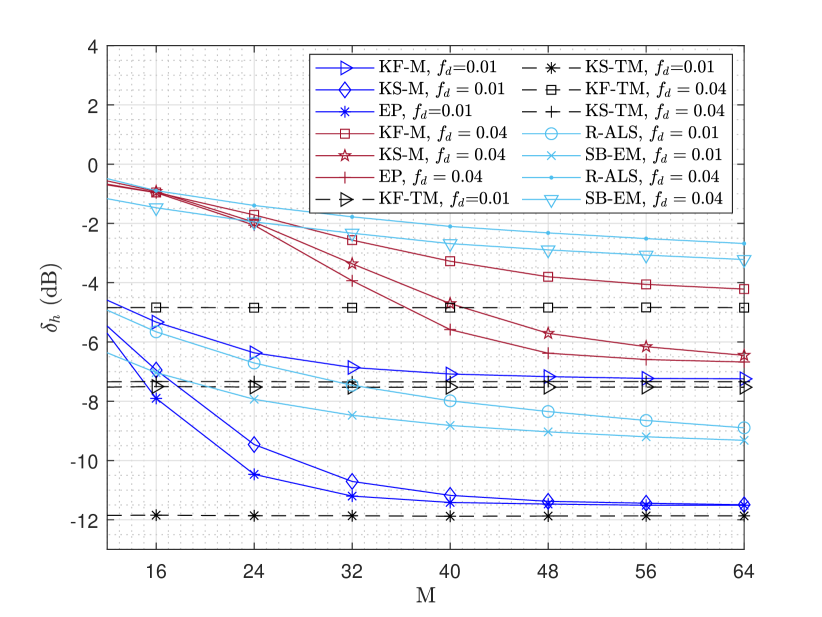
Figure 4: Channel estimation error versus the receiver’s antenna array size $M$ and with parameters: $K=8$, $T_{d}=64$, $T_{p}=K$, $a=0.1$, $\rho=0$.

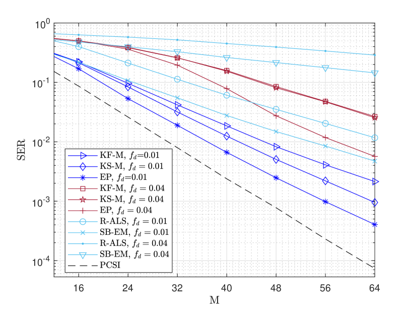
Figure 5: SER versus the receiver’s antenna array size $M$ and with parameters: $K=8$, $T_{d}=64$, $T_{p}=K$, $a=0.1$, $\rho=0$.

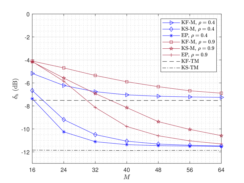
Figure 6: Channel estimation error versus the receiver’s antenna array size $M$ and with parameters: $K=8$, $T_{d}=64$, $T_{p}=K$, $a=0.1$, $f_{d}=0.01$.

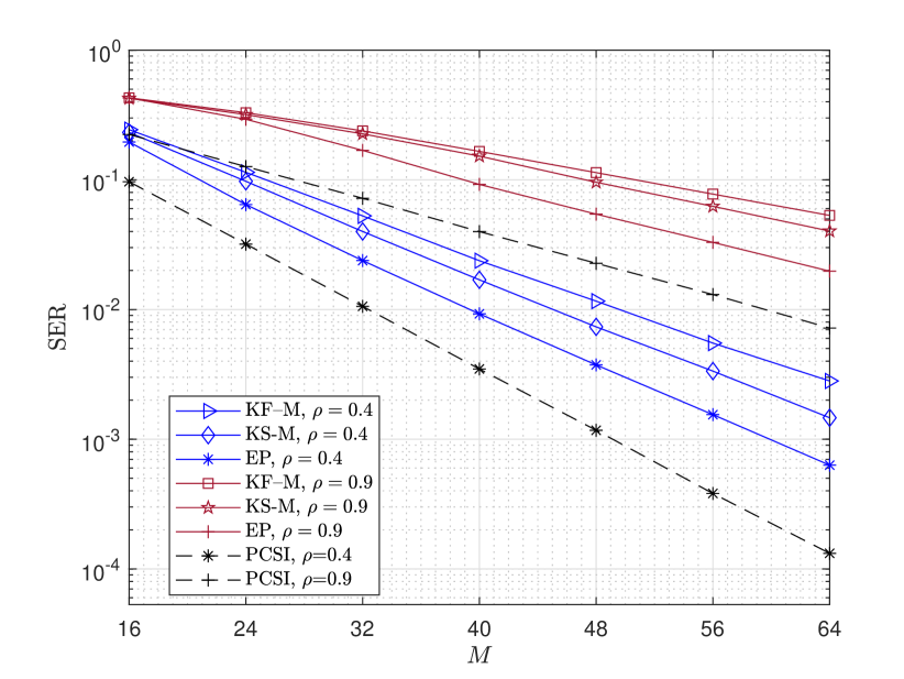
Figure 7: SER versus the receiver’s antenna array size $M$ and with parameters: $K=8$, $T_{d}=64$, $T_{p}=K$, $a=0.1$, $f_{d}=0.01$.

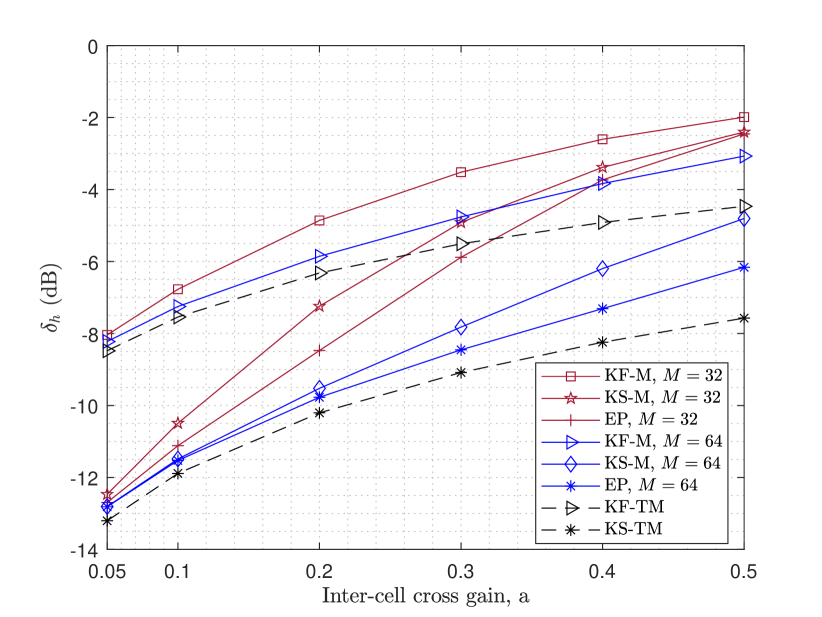
Figure 8: Channel estimation error versus the cross gain $a$ of users in other cells and with parameters: $K=8$, $T_{d}=64$, $T_{p}=K$, $f_{d}=0.01$, $\rho=0.4$.

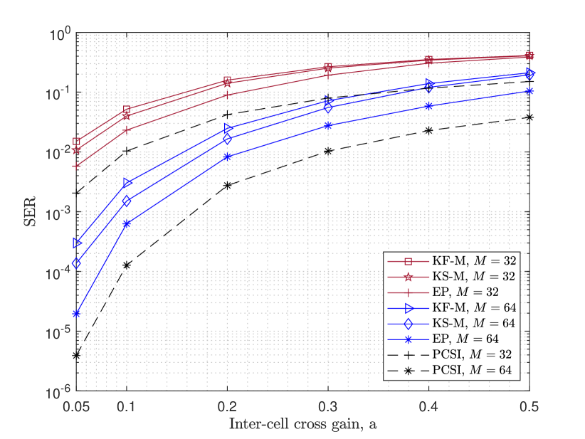
Figure 9: SER versus the cross gain $a$ of users in other cells and with parameters: $K=8$, $T_{d}=64$, $T_{p}=K$, $f_{d}=0.01$, $\rho=0.4$.

Fig. 5 shows the channel estimation error versus the number of antennas $M$ for KF-M, KS-M, and EP algorithms in a spatially uncorrelated ($\rho=0$) but temporally correlated channel. We consider two different cases for the temporal correlation corresponding to $f_{d}=0.01$ and $f_{d}=0.04$. We observe that in both of these cases the performance of the algorithms improves with $M$ and EP has a significant improvement over KF-M. The channel is more time-varying in the case of $f_{d}=0.04$ and the estimation error is higher in this case. The channel estimation error of KF-M approaches that of KF-TM for larger values of $M$ and the performance of EP approaches that of KS-TM. For both values of $f_{d}$, with increasing $M$ our proposed semi-blind EP algorithm converges faster to KS-TM than the semi-blind KS-M resulting in more accurate channel estimation. Note that while KF-TM and KS-TM algorithms employ $T=72$ pilot symbols to estimate the channel, KF-M, KS-M, and EP use only $T_{p}=K=8$ pilot symbols to estimate the channel (as well as detect $T_{d}=64$ data symbols). Channel estimation improvement with $M$ is a result of the so-called favorable propagation condition where the channel vectors of different users become mutually orthogonal as $M\longrightarrow\infty$. As a result, the performance of MMSE symbol estimator used in KF-M and EP improves. This in turn improves the channel estimation accuracy for KF-M, KS-M, and EP. Fig. 5 also shows the performance of the semi-blind expectation maximization (SB-EM) and the regularized alternating least-square (R-ALS) algorithms proposed in [10] and [12], respectively, for the channel described above using $T_{p}=8$ pilot symbols. We observe that for $f_{d}=0.01$, both SB-EM and R-ALS perform better than the KF-M and KF-TM algorithms, but worse than the KS-M and EP. The improvement in performance over KF-M and KF-TM is because both SB-EM and R-ALS estimate the channel using the entire received frame, whereas at any given time, KF-M and KF-TM update the channel estimates using the received signals up to the present time. Since KS-M, KS-TM, and EP use the entire received frame as well in a smoothing pass, they outperform SB-EM and R-ALS due to the underlying block-fading assumption of the latter two algorithms. Further, we observe that in the case of $f_{d}=0.04$, where the channel is highly time-varying, the performance of R-ALS and SB-EM is worse than all the other algorithms.

Fig. 5 depicts the SER performance of KF-M, KS-M, EP and PCSI versus the number of antennas $M$. We can see that for both values of $f_{d}$, the SER performance of all the algorithms improves with $M$ and EP outperforms all the other algorithms except for PCSI (MMSE with known channel coefficients). Moreover, the improvement of EP over the other algorithms increases with $M$. The SER performance of SB-EM and R-ALS is also shown in Fig. 5. It can be seen from Figs. 5 and 5 that the performance of algorithms developed under the block-fading assumption is significantly degraded when the algorithms are applied to time-varying channels as compared with algorithms specifically designed for such channels.

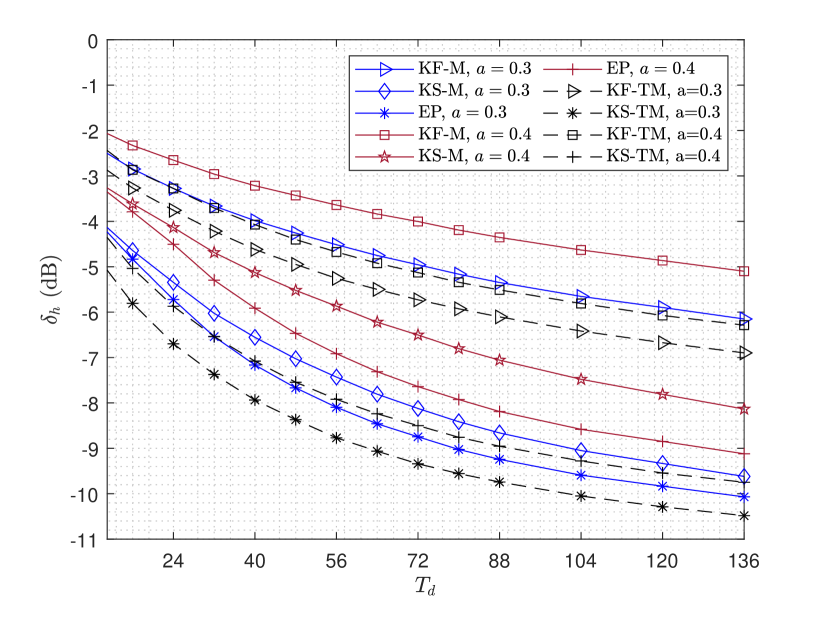
Figure 10: Channel estimation error versus $T_{d}$ and with parameters: $K=8$, $M=64$, $T_{p}=K$, $f_{d}=0.01$, $\rho=0.4$.

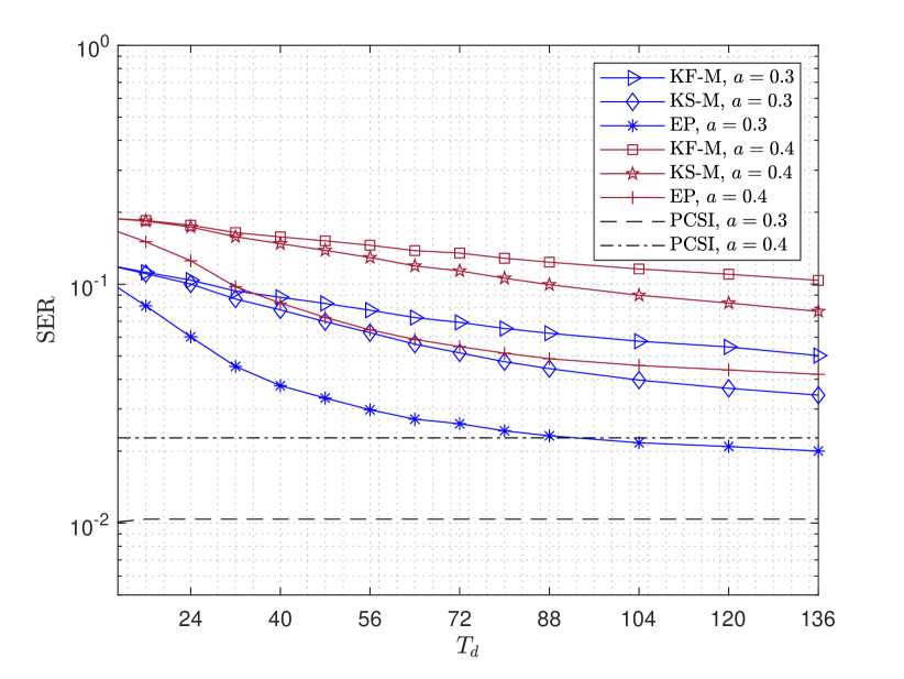
Figure 11: SER versus $T_{d}$ and with parameters: $K=8$, $M=64$, $T_{p}=K$, $f_{d}=0.01$, $\rho=0.4$.

Figure 12: Channel estimation error versus the normalized Doppler shift $f_{d}$ and with parameters: $K=8$, $M=64$, $T_{d}=64$, $\rho=0.4$, $a=0.3$.

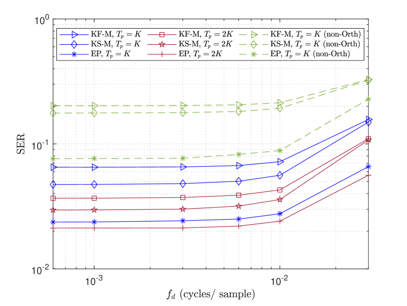
Figure 13: SER versus the normalized Doppler shift $f_{d}$ and with parameters: $K=8$, $M=64$, $T_{d}=64$, $\rho=0.4$, $a=0.3$.

Figs. 7 and 7 show the performance of KF-M, KS-M, and EP versus the number of antennas $M$ for a spatially and temporally correlated massive MIMO channel. For the case of $f_{d}=0.01$ we consider two different cases of spatial correlation corresponding to $\rho=0.4$ and $\rho=0.9$. We can see that in both cases the performance of the algorithms again improves with $M$ and EP significantly outperforms KF-M and KS-M. A comparison of the three cases for $\rho=0$ (in Figs. 5 and 5), $\rho=0.4$ and $\rho=0.9$ confirms the expected result that as $\rho$ increases, channel diversity decreases resulting in the degradation of system performance. In addition, spatial channel correlation reduced the level of channel hardening. In conclusion, as spatial correlation increases, a larger number of antennas are required to achieve the same level of performance [17].

In Figs. 9 and 9, we study the effect of pilot contamination on channel estimation error and SER. To this end, we vary the inter-cell cross gain $a$ between the BS in the first cell and the users in the three neighboring cells for the cases of $M=32,64$. As expected, as the cross gain $a$ increases, the performance of the algorithms degrades. However, as the figures show, EP significantly outperforms KF-M and KS-M. Moreover, there is a significant improvement as $M$ increases from $32$ to $64$.

Figs. 11 and 11 show the performance of the algorithms versus the number of data symbols $T_{d}$ in the transmitted frame. Two different cases of inter-cell interference described by $a=0.3$ and $a=0.4$ are considered. It is observed that as $T_{d}$ increases, the channel estimation error and SER performance of all algorithms improves. This improvement is due to the fact that the semi-blind approach uses the $T_{d}$ data symbols as virtual pilot symbols in estimating the channel. Thus for a fixed number of antennas $M$, using a large $T_{d}$ can mitigate the impact of pilot contamination [10]. In these figures, the improvement in EP’s performance is better than both KF-M and KS-M. This is due to the fact that EP updates the channel estimate at each time instant by incorporating the forward, reverse, and observation messages. In contrast, KF-M does not include the reverse and observation messages and KS-M does not include the observation messages. Hence as $T_{d}$ increases, the channel estimates found through the smoothing pass of EP are more accurate than those from KS-M and KF-M. Further, iterative forward and backward pass on the entire transmitted frame improves the SER performance of EP as well.

Finally, in Figs. 13 and 13, we study the performance of KF-M, KS-M, and EP versus the normalized Doppler shift $f_{d}$ for the pilot sequence of length $T_{p}=K$ and $T_{p}=2K$. It is seen that as $f_{d}$ increases (the temporal correlation among the channel vectors decreases), the performance of all algorithms degrades. It is interesting to note that for $f_{d}\leq 0.005$, the performance of the algorithms is almost constant with $f_{d}$. In essence for these values of $f_{d}$, the channel may be assumed to be time-invariant (block fading). For the parameters listed in foot.1, this translates to mobile velocities less than $20$ Km/h. In these figures we also show the performance of the algorithms when non-orthogonal pilot sequences for users in the first cell are used. In this case for each user $T_{p}$ QPSK symbols are randomly generated and used at the beginning of each frame as the pilot symbols. Although EP still outperforms KF-M and KS-M in this case, a degradation in performance is observed compared to the previous case for all the algorithms.

V Conclusions

In this paper, we propose a semi-blind expectation propagation (EP) based algorithm for joint channel estimation and symbol detection in the uplink of multi-cell massive MIMO systems for spatially and temporally correlated channels. EP algorithm is developed to approximate the a posteriori distribution of the channel matrix and data symbols with a distribution from an exponential family. The latter is then used to directly estimate the channel and detect the data symbols. A modified version of the classical Kalman filtering algorithm (referred to as KF-M) is also proposed that emerges from our EP derivations and is used in initializing the EP-based algorithm. Performance of Kalman Smoothing algorithm followed by KF-M (referred to as KS-M) is also examined. Simulation results show that the performance of KF-M, KS-M, and EP algorithms improves with the increase in the number of base station antennas $M$ and the length of the data symbols $T_{d}$ in the transmitted frame. Thus for a fixed $M$, using a large $T_{d}$ in the semi-blind approach can mitigate the effect of pilot contamination in multi-cell systems. Moreover, the EP-based algorithm significantly outperforming KF-M and KS-M algorithms. Finally, our results show that when applied to time-varying channels, these algorithms outperform the algorithms that are developed for block-fading channel models.

References

- [1] O. Elijah, C. Y. Leow, T. A. Rahman, S. Nunoo, and S. Z. Iliya, “A comprehensive survey of pilot contamination in massive MIMO-5G system,” IEEE Communications Surveys Tutorials, vol. 18, no. 2, pp. 905–923, Secondquarter 2016.
- [2] K. Ghavami and M. Naraghi-Pour, “Blind channel estimation and symbol detection for Multi-Cell Massive MIMO systems by expectation propagation,” IEEE Transactions on Wireless Communications, vol. 17, no. 2, pp. 943–954, Feb 2018.
- [3] J. Zhang, X. Yuan, and Y. A. Zhang, “Blind signal detection in massive MIMO: Exploiting the channel sparsity,” IEEE Transactions on Communications, vol. 66, no. 2, pp. 700–712, Feb 2018.
- [4] L. Chen and X. Yuan, “Blind multiuser detection in massive MIMO channels with clustered sparsity,” IEEE Wireless Communications Letters, vol. 8, no. 4, pp. 1052–1055, 2019.
- [5] A. Mezghani and A. L. Swindlehurst, “Blind estimation of sparse broadband massive MIMO channels with ideal and one-bit ADCs,” IEEE Transactions on Signal Processing, vol. 66, no. 11, pp. 2972–2983, 2018.
- [6] T. P. Minka, “Expectation propagation for approximate bayesian inference,” in Proceedings of the Seventeenth Conference on Uncertainty in Artificial Intelligence, San Francisco, CA, USA, 2001, pp. 362–369.
- [7] H. Liu, X. Yuan, and Y. J. Zhang, “Super-Resolution Blind Channel-and-Signal Estimation for Massive MIMO With One-Dimensional Antenna Array,” IEEE Transactions on Signal Processing, vol. 67, no. 17, pp. 4433–4448, 2019.
- [8] E. De Carvalho and D. T. M. Slock, “Cramer-Rao bounds for semi-blind, blind and training sequence based channel estimation,” in First IEEE Signal Processing Workshop on Signal Processing Advances in Wireless Communications, 1997, pp. 129–132.
- [9] K. Mawatwal, D. Sen, and R. Roy, “A semi-blind channel estimation algorithm for massive MIMO systems,” IEEE Wireless Communications Letters, vol. 6, no. 1, pp. 70–73, Feb 2017.
- [10] E. Nayebi and B. D. Rao, “Semi-blind channel estimation for multiuser massive MIMO systems,” IEEE Transactions on Signal Processing, vol. 66, no. 2, pp. 540–553, Jan 2018.
- [11] D. Hu, L. He, and X. Wang, “Semi-blind pilot decontamination for massive MIMO systems,” IEEE Transactions on Wireless Communications, vol. 15, no. 1, pp. 525–536, Jan 2016.
- [12] S. Liang, X. Wang, and L. Ping, “Semi-Blind Detection in Hybrid Massive MIMO Systems via Low-Rank Matrix Completion,” IEEE Transactions on Wireless Communications, vol. 18, no. 11, pp. 5242–5254, 2019.
- [13] B. Srinivas, K. Mawatwal, D. Sen, and S. Chakrabarti, “A semi-blind based channel estimator for pilot contaminated one-bit massive MIMO systems,” in 2018 IEEE 88th Vehicular Technology Conference (VTC-Fall), Aug 2018, pp. 1–7.
- [14] W. Yan and X. Yuan, “Semi-Blind Channel-and-Signal Estimation for Uplink Massive MIMO With Channel Sparsity,” IEEE Access, vol. 7, pp. 95 008–95 020, 2019.
- [15] L. Li and Z. Wang, “A novel spatial correlation estimation technique for mimo communication system,” in IEEE Vehicular Technology Conference, 2006, pp. 1–5.
- [16] L. Yang and J. Qin, “Performance of stbcs with antenna selection: spatial correlation and keyhole effects,” IEE Proceedings - Communications, vol. 153, no. 1, pp. 15–20, 2006.
- [17] E. Björnson, J. Hoydis, and L. Sanguinetti, Massive MIMO Networks: Spectral, Energy, and Hardware Efficiency, 2017.
- [18] A. K. Papazafeiropoulos and T. Ratnarajah, “Deterministic equivalent performance analysis of time-varying massive MIMO systems,” IEEE Transactions on Wireless Communications, vol. 14, no. 10, pp. 5795–5809, Oct 2015.
- [19] R. Chopra, C. R. Murthy, H. A. Suraweera, and E. G. Larsson, “Performance analysis of FDD massive MIMO systems under channel aging,” IEEE Transactions on Wireless Communications, vol. 17, no. 2, pp. 1094–1108, Feb 2018.
- [20] A. K. Papazafeiropoulos, “Impact of General Channel Aging Conditions on the Downlink Performance of Massive MIMO,” IEEE Transactions on Vehicular Technology, vol. 66, no. 2, pp. 1428–1442, 2017.
- [21] K. T. Truong and R. W. Heath, “Effects of channel aging in massive MIMO systems,” Journal of Communications and Networks, vol. 15, no. 4, pp. 338–351, 2013.
- [22] W. C. Jakes and D. C. Cox, Microwave Mobile Communications. Wiley-IEEE Press, 1994.
- [23] S. Srivastava, A. Mishra, A. Rajoriya, A. K. Jagannatham, and G. Ascheid, “Quasi-Static and Time-Selective Channel Estimation for Block-Sparse Millimeter Wave Hybrid MIMO Systems: Sparse Bayesian Learning (SBL) Based Approaches,” IEEE Transactions on Signal Processing, vol. 67, no. 5, pp. 1251–1266, 2019.
- [24] S. Kashyap, C. Mollén, E. Björnson, and E. G. Larsson, “Performance analysis of (TDD) massive MIMO with Kalman channel prediction,” in 2017 IEEE International Conference on Acoustics, Speech and Signal Processing (ICASSP), March 2017, pp. 3554–3558.
- [25] A. Almamori and S. Mohan, “Estimation of channel state information for massive MIMO based on received data using Kalman filter,” in 2018 IEEE 8th Annual Computing and Communication Workshop and Conference (CCWC), 2018, pp. 665–669.
- [26] A. Forenza, D. J. Love, and R. W. Heath, “Simplified Spatial Correlation Models for Clustered MIMO Channels With Different Array Configurations,” IEEE Transactions on Vehicular Technology, vol. 56, no. 4, pp. 1924–1934, 2007.
- [27] Da-Shan Shiu, G. J. Foschini, M. J. Gans, and J. M. Kahn, “Fading correlation and its effect on the capacity of multielement antenna systems,” IEEE Transactions on Communications, vol. 48, no. 3, pp. 502–513, 2000.
- [28] K. E. Baddour and N. C. Beaulieu, “Autoregressive modeling for fading channel simulation,” IEEE Transactions on Wireless Communications, vol. 4, no. 4, pp. 1650–1662, July 2005.
- [29] M. K. Tsatsanis, G. B. Giannakis, and G. Zhou, “Estimation and equalization of fading channels with random coefficients,” in 1996 IEEE International Conference on Acoustics, Speech, and Signal Processing Conference Proceedings, vol. 2, May 1996, pp. 1093–1096.
- [30] C. Komninakis, C. Fragouli, A. H. Sayed, and R. D. Wesel, “Multi-input multi-output fading channel tracking and equalization using Kalman estimation,” IEEE Transactions on Signal Processing, vol. 50, no. 5, pp. 1065–1076, May 2002.
- [31] Y. Qi and T. P. Minka, “Window-based expectation propagation for adaptive signal detection in flat-fading channels,” IEEE Transactions on Wireless Communications, vol. 6, no. 1, pp. 348–355, Jan 2007.
- [32] T. P. Minka, “A family of algorithms for approximate bayesian inference,” Ph.D. dissertation, Massachusetts Institute of Technology, Cambridge, MA, USA, 2001.
- [33] K. Ghavami and M. Naraghi-Pour, “MIMO detection with imperfect channel state information using expectation propagation,” IEEE Transactions on Vehicular Technology, vol. 66, no. 9, pp. 8129–8138, Sep. 2017.
- [34] H. Q. Ngo, T. L. Marzetta, and E. G. Larsson, “Analysis of the pilot contamination effect in very large multicell multiuser MIMO systems for physical channel models,” in 2011 IEEE International Conference on Acoustics, Speech and Signal Processing (ICASSP), 2011, pp. 3464–3467.
- [35] H. Q. Ngo, E. G. Larsson, and T. L. Marzetta, “The Multicell Multiuser MIMO Uplink with Very Large Antenna Arrays and a Finite-Dimensional Channel,” IEEE Transactions on Communications, vol. 61, no. 6, pp. 2350–2361, 2013.
- [36] E. Björnson, J. Hoydis, and L. Sanguinetti, “Massive MIMO Networks: Spectral, Energy, and Hardware Efficiency,” Foundations and Trends® in Signal Processing, vol. 11, no. 3-4, pp. 154–655, 2017. [Online]. Available: http://dx.doi.org/10.1561/2000000093
- [37] T. Kim, “User scheduling and grouping in massive MIMO broadcast channels with heterogeneous users,” Journal of Communications and Networks, vol. 21, no. 4, pp. 385–394, 2019.