Improved Fe ii emission line models for AGN using new atomic datasets

Abstract

Understanding the Fe ii emission from Active Galactic Nuclei (AGN) has been a grand challenge for many decades. The rewards from understanding the AGN spectra would be immense, involving both quasar classification schemes such as “Eigenvector 1” and tracing the chemical evolution of the cosmos. Recently, three large Fe ii atomic datasets with radiative and electron collisional rates have become available. We have incorporated these into the spectral synthesis code Cloudy and examine predictions using a new generation of AGN Spectral Energy Distribution (SED), which indicates that the UV emission can be quite different depending on the dataset utilised. The Smyth et al dataset better reproduces the observed Fe ii template of the $\rm\thinspace I\rm\thinspace ZW\rm\thinspace 1$ Seyfert galaxy in the UV and optical regions, and we adopt these data. We consider both thermal and microturbulent clouds and show that a microturbulence of $\approx$ 100 km/s reproduces the observed shape and strength of the so-called Fe ii “UV bump”. Comparing our predictions with the observed Fe ii template, we derive a typical cloud density of $10^{11}$ cm^-3 and photon flux of $10^{20}$ cm^-2 s^-1, and show that these largely reproduce the observed Fe ii emission in the UV and optical. We calculate the $I(\mbox{{\rm Fe~{}{\sc ii}}})/I(\mbox{{\rm Mg~{}{\sc ii}}})$ emission-line intensity ratio using our best-fitting model and obtain log($I(\mbox{{\rm Fe~{}{\sc ii}}})/I(\mbox{{\rm Mg~{}{\sc ii}}})$) $\sim$ 0.7, suggesting many AGNs have a roughly solar Fe/Mg abundance ratio. Finally, we vary the Eddington ratio and SED shape as a step in understanding the Eigenvector 1 correlation.

1 Introduction

Emission lines of Fe ii are a major contributor to the AGN spectra, with wavelengths spanning the infrared (IR) to ultraviolet (UV) regions. These emission lines provide an important laboratory for developing Fe ii as a physical and geometrical diagnostic for the broad–line regions (BLRs) in AGN. Understanding the physics behind the Fe ii emission is important for multiple reasons. It is the primary indicator of Eigenvector 1 (EV1), a key property to construct the quasar main sequence (e.g., Boroson & Green, 1992; Sulentic et al., 2000; Marziani et al., 2001). EV1, which relates to the black hole mass and quasar orientation (e.g., Shen & Ho, 2014; Panda et al., 2018, 2019), shows a strong anti-correlation with optical Fe ii equivalent width in the Seyfert galaxies and quasars. Recent work shows correlations between the line widths of optical Fe ii and UV Fe ii in quasar spectra, which indicates that the emitting regions are close together (Kovačević-Dojčinović & Popović, 2015). It may be that both are emitted from the outer region of BLR or intermediate-line region (ILR).

Strong Fe ii emission is also useful to investigate the energy budget of the emitting gas. The iron abundance as a function of cosmic time allows us to verify several cosmological parameters (Hamann & Ferland, 1999). In most galaxy evolution models, iron is mainly deposited in the interstellar medium (ISM) through Type Ia supernovae (SNIa), which occur about 0.3 to 1 billion years after the initial burst of star formation, because for Type Ia supernovae to occur the galaxy has to be old enough to host white dwarfs. This triggers a sudden jump in the iron abundance, as shown in Hamann & Ferland (1999) and Matteucci & Recchi (2001). The Gunn-Peterson effect in quasars suggests that the most recent onset of star formation occurred around $z\ \sim$ 6 (e.g., Djorgovski et al., 2001; Fan et al., 2006; Bolton & Haehnelt, 2007; Kim et al., 2009; Sarkar & Samui, 2019). A properly calibrated iron chronometer would allow us to measure the iron abundance at high redshift, offering the possibility of measuring the redshift when Type Ia supernovae first happened (Baldwin et al., 2004).

The timescale for iron enrichment in the ISM is much longer than that of $\alpha$-elements, such as- magnesium. Magnesium is deposited in the ISM via core-collapsed (Type II) supernovae, which have much shorter timescales than Type I. The flux ratio of UV Fe ii multiplet to the $\mbox{{\rm Mg~{}{\sc ii}}}\ \lambda$2800 doublet (hereafter $I(\mbox{{\rm Fe~{}{\sc ii}}})/I(\mbox{{\rm Mg~{}{\sc ii}}})$) of quasars, therefore lets us probe the material deposited through Type Ia supernovae versus that processed through $\alpha$-process in stars and then ejected via Type II supernovae (e.g., Kurk et al., 2007; De Rosa et al., 2011; Wu et al., 2015; Mazzucchelli et al., 2017; Shin et al., 2019). Thus, the $I(\mbox{{\rm Fe~{}{\sc ii}}})/I(\mbox{{\rm Mg~{}{\sc ii}}})$ ratio provides a powerful approach to investigate the chemical evolution of AGNs.

The theoretical and observational aspects of Fe ii emission have been long-standing and important problems addressed by Osterbrock (1977); Phillips (1978); Netzer & Wills (1983); Wills et al. (1985); Verner et al. (1999); Baldwin et al. (2004) due to its great strength in many Seyfert galaxies and quasars. Previous work with collisional excitation of Fe ii in the framework of photoionization models failed to reproduce the observed strength of Fe ii emission in the UV. The observed Fe ii spectra of narrow-line Seyfert galaxies (e.g., Vestergaard & Wilkes, 2001) contain a so called “UV bump” between the $\mbox{{\rm C~{}{\sc iii}}}\ \lambda$1909 and $\mbox{{\rm Mg~{}{\sc ii}}}\ \lambda$2800 emission lines (Baldwin et al., 2004), which is produced by blending of a large number of Fe ii emission lines due to transitions between high-lying states with energies E $\geq$ 13.25 eV (e.g., Leighly et al., 2007; Bruhweiler & Verner, 2008). However, the collisional excitation models (Kwan & Krolik, 1981) only predict an electron temperature of T $\leq$ $10^{4}$ K at the illuminating faces of the Fe ii emitting cloud which is too low to excite electrons to the high-lying energy levels (E $\geq$ 8 eV).

Wills et al. (1985) first pointed out the importance of continuum fluorescence to excite the electrons to the higher energy states (E $\geq$ 11.6 eV). Several spectral energy distributions (SEDs) of AGN with increasing Eddington ratio (L/L_Edd) have been proposed to reproduce the observed shape of the Fe ii UV bump, where L_Edd is the Eddington luminosity of the corresponding AGN (e.g., Mathews & Ferland, 1987; Korista et al., 1997; Jin et al., 2012). However, the Fe ii atomic dataset has long remained a concern for reproducing Fe ii spectra. A larger Fe ii model involves a large number of transitions between the high-lying energy states, producing stronger Fe ii emission in the UV.

We have incorporated three recent Fe ii datasets, namely those of Bautista et al. (2015), Tayal & Zatsarinny (2018), and Smyth et al. (2019) into the spectral synthesis code Cloudy (Ferland et al., 2017) in addition to the Mathews & Ferland (1987), Korista et al. (1997), and Jin et al. (2012) AGN SEDs. Our model predictions are compared with the observed UV (Vestergaard & Wilkes, 2001) and optical (Véron-Cetty et al., 2004) BLR templates of 1 ZW I Seyfert galaxy to constrain the physical conditions and geometrical properties of the Fe ii emitting gas. We find that the Smyth et al. (2019) Fe ii dataset, the Jin et al. (2012) SED, and a dense turbulent cloud, largely reproduce the Fe II emission with solar abundances.

Our goal is to reproduce the shape and strength of the Fe ii UV bump and optical emission. We study the emission from a single BLR cloud in some detail. The emission lines are known to be formed in a distribution of clouds with different locations and densities. This was first measured with reverberation (Peterson, 1993) and is a consequence of atomic physics selection effects (Baldwin et al., 1995). This must be taken into account when emission from different species with a broad range of ionization potential or critical density is considered. However, emission from one particular species is generally localized to favored values of the density and ionizing photon flux, as illustrated by Korista et al. (1997) and Baldwin et al. (2004), so, when considering a single species like Fe ii, a typical set of cloud parameters can be considered, as in Ferland et al. (2009). We compare Fe ii and Mg ii emissions later in the paper because these species are used as abundance indicators in high-redshift quasars. Figure 3f of Korista et al. (1997) shows that Fe ii and Mg ii lines form in very similar clouds, justifying this approach.

There are also complex interplays between different sets of model parameters such as turbulence, the SED shape, or composition. Our primary goal is to develop a testing framework to compare theory and observations, and to document the spectral properties of these new atomic data sets. The new Fe ii atomic data files, and the infrastructure needed to use them, will be included in the C17.03 update to Cloudy and we hope that the analysis methods we demonstrate here can serve as a guide for future studies and detailed comparisons with observations.

We assume solar abundances. Studies of high-ionization lines find that the metallicity is above solar and correlates with luminosity (Hamann & Ferland, 1999). Recently Schindler et al. (2020) measured the Fe ii/Mg ii ratio of a large number of quasars across cosmic time. They did not find any evolution and concluded that the ratios were consistent with solar abundances. In later sections of the paper we show that this line ratio has only a weak metallicity dependence. For simplicity, we assume solar abundances in the calculations presented here.

Finally, we adopt a cosmology of $H_{0}$ = 70 km s^-1 Mpc^-1, $\Omega_{\Lambda}$ = 0.7, and $\Omega_{m}$ = 0.3.

2 Basic ingredients

A complete model of the physical processes that affect the Fe ii spectrum would help us to constrain the gas properties and dynamics in the BLR. However, difficulties arise because a variety of processes determine the observed Fe ii emission, such as collisional excitation, pumping by the continuum photons, and fluorescence via line overlap. The spectral energy distribution (SED) of the background AGN, the cloud’s density, turbulence, and optical depth of the gas also play important roles. A realistic model should take into account all those effects while modeling the temperature and ionization structure of the gas.

We use the development version of Cloudy , last described by Ferland et al. (2017). We adopt Cloudy’s default solar composition, as listed in Table 1.

Table 1: Solar abundances used in Cloudy

Elements	Abundances	Elements	Abundances
H	1.0	S	1.84e-5
He	0.10	Cl	1.91e-7
Li	2.04e-9	Ar	2.51e-6
Be	2.63e-11	K	1.32e-7
B	6.17e-10	Ca	2.29e-6
C	2.45e-4	Sc	1.48e-9
N	8.51e-5	Ti	1.05e-7
O	4.90e-4	V	1.00e-8
F	3.02e-8	Cr	4.68e-7
Ne	1.00e-4	Mn	2.88e-7
Na	2.14e-6	Fe	2.82e-5
Mg	3.47e-5	Co	8.32e-8
Al	2.95e-6	Ni	1.78e-6
Si	3.47e-5	Cu	1.62e-8
P	3.20e-7	Zn	3.98e-8

Note. — Solar abundances of different elements relative to H, incorporated in Cloudy–C17. Abundances of most elements are taken from Grevesse & Sauval (1998), except for C, O which are taken from Allende Prieto et al. (2002), and N, Ne, Si, Mg, Fe are taken from Holweger (2001).

2.1 Fe ii atomic datasets

The Fe ii ion has a complex structure with 25 electrons, and is a “grand challenge” problem in atomic physics. An accurate set of radiative and collisional atomic data is therefore needed to treat the selective excitation, continuum pumping, and fluorescence, which are known to be important for the Fe ii emission (e.g., Baldwin et al., 2004; Bruhweiler & Verner, 2008; Jin et al., 2012; Wang et al., 2016; Netzer, 2020). Uncertainties in the atomic data have been a longstanding limitation in interpreting line intensities. Below we discuss four different Fe ii atomic datasets that are now available in the Cloudy, while their energy levels are compared in Figure 1.

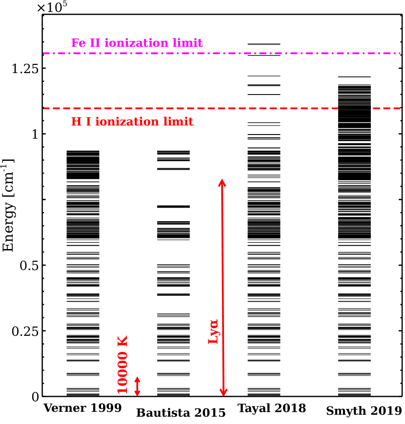
Figure 1: Diagram showing the energy levels of various models of the Fe ii atom. From left to right : dataset derived by Verner et al. (1999), Bautista et al. (2015), Tayal & Zatsarinny (2018), and Smyth et al. (2019). The horizontal dashed lines indicate the H i and Fe ii ionization limits. The energy of the Ly$\alpha$ transition, an important source of photoexcitation of Fe ii, is also indicated, along with the thermal energy corresponding to 10⁴ K.

First, we consider the widely used Verner et al. (1999) Fe ii dataset with 371 atomic levels producing 13,157 emission lines with a highest energy level of $\sim$ 11.6 eV. Verner et al. (1999) data has collision strengths mainly calculated from the “g-bar” approximation. The original paper presented a total of $\sim 68,000$ transitions in their model atom. Most of these transitions are strongly forbidden and are assigned very small transition rates. Transition probabilities between their energy levels have uncertainties $\mathrel{\hbox{\hbox to0.0pt{\hbox{\lower 4.0pt\hbox{$\sim$}}\hss}\hbox{$<$}}}$ 20% for strong permitted lines and $\mathrel{\hbox{\hbox to0.0pt{\hbox{\lower 4.0pt\hbox{$\sim$}}\hss}\hbox{$>$}}}$ 50% for weak permitted and inter-combination lines. Also, forbidden lines have uncertainties $\mathrel{\hbox{\hbox to0.0pt{\hbox{\lower 4.0pt\hbox{$\sim$}}\hss}\hbox{$<$}}}$ 50%. We exclude all the totally forbidden lines from the $68,000$ transitions because of their small transition rates. Figure 1 shows the energy levels predicted by the Verner et al. (1999) Fe ii model.

Bautista et al. (2015) reports a Fe ii model with 159 levels extending up to 11.56 eV, producing 628 emission lines. Uncertainties in the transition probabilities lie between 10% and 30%. Tests show that the Bautista et al. (2015) Fe ii dataset has no lines between 2000Å  and 3000Å. As our paper mainly focuses on the UV band (2000Å– 3000Å) in Fe ii spectra, we do not use this data-set for our BLR modelling.

Tayal & Zatsarinny (2018) calculate 340 energy levels with a highest energy of $\sim$ 16.6 eV, including all levels from the $3d^{6}4s$, $3d^{5}4s^{2}$, $3d^{7}$, $3d^{6}4p$ configurations and a few levels from the $3d^{5}4s4p$ configuration. Transitions between these energy levels produce 57,635 emission lines with uncertainties in transition probabilities of $\mathrel{\hbox{\hbox to0.0pt{\hbox{\lower 4.0pt\hbox{$\sim$}}\hss}\hbox{$<$}}}$ 30% (in the 2200Å–7800Å). This dataset contains autoionizing levels with E $>$ 13.6 eV, which are absent in Verner et al. (1999) and Bautista et al. (2015). However, the density of states in high-lying energy levels are low, as shown in Figure 1.

Another larger Fe ii data-set is also recently available in Cloudy. Smyth et al. (2019) compute energy levels taking into account 216 $LS$ terms in Fe ii atom arising from the $3d^{6}4s$, $3d^{7}$, $3d^{6}4p$, $3d^{5}4s^{2}$, and $3d^{5}4s4p$ configurations. The Smyth et al. (2019) model has considerably more configurations (see pg 657) in the structure but only includes 716 levels in the close coupling (scattering model), with the highest energy level reaching 26.4 eV. These levels produce 255,974 emission lines. The Smyth et al. (2019) dataset also contains autoionizing levels, but the density of states in the high-lying energy states is large compared to Tayal & Zatsarinny (2018).

We model the Fe ii emitting cloud using Verner et al. (1999), Tayal & Zatsarinny (2018), and Smyth et al. (2019) and compare their predictions. Results are discussed in Section 3.

2.2 AGN SEDs

The BLR spectra in AGN mostly originate from the gas clouds photoionized by continuum radiation coming from an accretion disk around the central black hole. An accurate SED from the UV through to the soft X-ray band is therefore important to understand the Fe ii emission (e.g., Wills et al., 1985; Verner et al., 1999; Korista et al., 1997; Wills et al., 1985; Baldwin et al., 2004; Bruhweiler & Verner, 2008; Jin et al., 2012; Wang et al., 2016; Netzer, 2020). The soft X-ray part of the SED can penetrate into low ionization regions to heat the gas and produce the Fe ii emission by thermal collisions. We consider the three SEDs presented by Mathews & Ferland (1987), Korista et al. (1997), and Jin et al. (2012), as shown in Figure 2. These have been normalised to have the same flux of ionizing photons, $\phi({\rm H}^{0})=10^{20}$ cm^-2 s^-1.

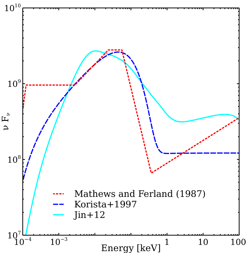
Figure 2: Comparing different SEDs used in Cloudy. Red dashed line: SED dervived by Mathews & Ferland (1987). Blue dashed line: SED derived by Korista et al. (1997). Cyan solid line: Jin et al. (2012) SED.

Figure 3: Comparing Cloudy predicted Fe ii spectra in 0.1–0.58 $\mu$m wavelength band using three different Fe ii datasets and a fixed SED (Jin et al., 2012). Red dotted line: Fe ii spectra using Verner et al. (1999) dataset. Blue dashed line: Tayal & Zatsarinny (2018) dataset. Cyan solid line: Smyth et al. (2019) dataset. Ranges of y-axis are different in all sub-figures.

Mathews & Ferland (1987) derived a simple and phenomenological SED extending from the infrared (0.00124 eV) through the hard X-ray (10⁵ eV), as shown in Figure 2. The shape of the continuum is approximated as a series of broken power-laws, i.e -

$${\rm f}_{\nu}={\rm a}{\nu}^{-\alpha},$$

where $\alpha$ is the spectral index. This can be determined by fitting the observed continuum with the power-law model in various energy bands.

We consider another standard SED derived in Korista et al. (1997), as shown in Figure 2. This is a baseline ionizing continuum model widely used to predict a wide range of emission lines in quasars (e.g., Ruff et al., 2012; Marziani & Sulentic, 2014; Marinucci et al., 2018; Temple et al., 2020). The derived shape of the continuum is a combination of a UV bump and an X-ray power law, i.e.,

$${\rm f}_{\nu}={\nu}^{-0.5}{\rm exp}(-{\rm h}{\nu}/{\rm kT}_{\rm{UV}}){\rm exp}(-{\rm kT}_{\rm IR}/{\rm h}{\nu})+{\rm a}{\nu}^{-1},$$

where T_UV and T_IR are the cut-off temperatures of the UV bump and X-ray power law, respectively. The value of ‘a’ can be determined from the ratio of the UV to X-ray continua, defined as-

$$\frac{{\rm f}_{\nu}(2\ {\rm keV})}{{\rm f}_{\nu}(2500{\rm\thinspace\AA})}=403.3^{\alpha_{\rm ox}},$$

where $\alpha_{\rm ox}$ distinguishes the continua between different type of AGNs. As an example, for Type I Seyfert galaxies, $\alpha_{\rm ox}=-1.2$. The shape of the continuum in the Figure 2 corresponds to a UV bump peaking at $\sim$ 44 ${\rm\thinspace eV}$ and an exponential decay part with a slope of $-2.3$.

We also consider the new generation of SEDs which use the Eddington ratio (L/L_Edd) as parameter and are presented in Jin et al. (2012) and summarized by Ferland et al. (2020). These SEDs are a combination of theory and more recent observations. The SED with a log L/L_Edd = $-$0.55 is shown in Figure 2. The derived SED has three components, namely (1) AGN disk emission, (2) Comptonization, and (3) a high energy power law tail (Done et al., 2012). Figure 2 represents the shape of the broadband SED. It increases as blackbody emission (emission from the outer disk) from lower energy, peaks in the UV, then falls off due to inverse Compton scattering in the inner disk and finally attains a power law tail which is due to the inverse Compton scattering in the corona. As shown, the SEDs are normalized to have the same total number of ionizing photons. Note that they disagree by $\sim 1$ dex in the soft X-ray region.

We next use all three SEDs in Cloudy and compare their predicted Fe ii spectra.

Figure 4: Comparing Cloudy predicted Fe ii spectra in 0.1–0.58 $\mu$m wavelength bands using three different AGN SEDs and a fixed Fe ii dataset (Smyth et al., 2019). Red dotted line: Fe ii spectra using Mathews & Ferland (1987) SED. Blue dashed line: Korista et al. (1997) SED. Cyan solid line: Jin et al. (2012) SED. Ranges of y-axis are different in all sub-figures.

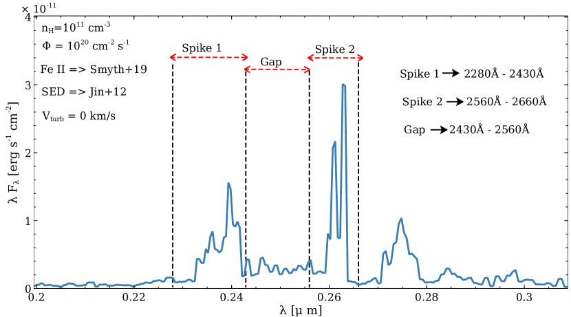
Figure 5: Blue spectrum shows a typical Fe ii spectra in UV using Smyth et al. (2019) dataset, Jin et al. (2012) SED. The Spikes and Gap are marked with vertical dashed lines.

3 Applications

3.1 Modelling of the BLR cloud

We model the BLR gas by assuming solar abundances, as listed in table 1, and a cloud column density (N_H) of $10^{24}$ cm^-2. First, we consider the Fe ii emission from a single cloud modelled using the Verner et al. (1999), Tayal & Zatsarinny (2018), and Smyth et al. (2019) datasets in addition to an intermediate L/L_Edd AGN SED, as described in Jin et al. (2012). Figure 3 compares the resulting Fe ii emission spectra for the different atomic datasets in the UV and optical. In both spectral ranges, the Smyth et al. (2019) Fe ii data-set produces larger line intensities compared to the other two. The Smyth et al. (2019) data-set has more very highly excited states that connect by permitted transitions to low-excitation highly-populated levels. Continuum fluorescent excitation is much stronger as a result, which brings the short-wavelength lines into better agreement with the template. The Smyth et al. (2019) dataset also better reproduces the observed Fe ii pseudo-continuum, which results from the blending of a large number of high-lying lines in the UV and optical (Garcia-Rissmann et al., 2012). We therefore select the Smyth et al. (2019) dataset to generate Fe ii emission lines throughout the remainder of this paper.

Figure 6: Contour plot of the Spike/gap ratio and equivalent width (EW) derived from photoionization model using the Smyth et al. (2019) Fe ii dataset and Jin et al. (2012) AGN SED. Left: Spike/gap ratio of the Fe ii UV bump in the n_H – $\Phi$ plane. Right: EW of Fe ii UV bump in the n_H – $\Phi$ plane. An axis indicating the distance of Fe ii emitting cloud from the central black hole is also added.

To find a suitable AGN SED for our BLR model, we predict Fe ii spectra using the Mathews & Ferland (1987), Korista et al. (1997), and Jin et al. (2012) SEDs in addition to the Smyth et al. (2019) Fe ii dataset. Figure 4 compares the Fe ii emission spectra for all three AGN SEDs we consider. The adopted density, flux, and turbulence parameters indicated in the figures as are the best-fitting parameters derived below.

The Mathews & Ferland (1987) and Korista et al. (1997) SEDs were simple empirical fits with little physical basis. In contrast, Jin et al. (2012) SED does have a theoretical foundation, as explained in the original papers, and that family of SEDs produce significantly more soft X-ray emission between $\sim$ 100 ${\rm\thinspace eV}$ to 1 ${\rm\thinspace keV}$ (see Figure 2) than the empirical SEDs. Soft X-rays are important because these higher energy photons can penetrate further into the cloud, deposit more energy in neutral gas, and produce stronger Fe ii lines by collisional excitation. Softer XUV and EUV photons are extinguished at shallower depth into the cloud, where Fe is more highly ionized, while hard X-rays and gamma-rays encounter less opacity so are transmitted without being reprocessed into emission lines.

The two older SEDs are shown in Figure 4 for historical reference. The papers describing them are highly cited (Mathews & Ferland 1987 and Korista et al. 1997) and they are built into Cloudy. Several studies have used these SEDs, and the Verner et al. (1999) atomic data set, to investigate emission properties of AGN. Although the older SEDs and the Verner et al. (1999) data have historical interest, we prefer the modern SED (Jin et al., 2012) with its foundation of observations and theory and the new generation of atomic data (Smyth et al., 2019) with more complete collision strengths.

For these reasons, we, therefore, adopt the Jin et al. (2012) SED for our BLR model throughout this paper. Additionally, the log L/L_Edd value for Jin et al. (2012) SED is consistent with that of $\rm\thinspace I\rm\thinspace ZW\rm\thinspace 1$ ($\gtrsim$ $-$0.60, Cracco et al., 2016; Giustini & Proga, 2019). This is the intermediate L/L_Edd SED and in Section 3.4 we explore the effects of varying L/L_Edd. We note that Cloudy makes it easy to adopt user-defined SEDs in new calculations. It is hope that the work we present here will lead to further explorations of the effects of the SED upon the line spectrum.

With the above selections of Fe ii dataset and SED, the remaining parameters are the cloud hydrogen density (n_H) and the flux of incoming photons striking the cloud ($\Phi$). We estimate these by considering a grid of photoionization models by varying these two parameters over a broad range.

The computed Fe ii spectra without microturbulence always show two prominent spikes at $\sim$ 2400Å and 2600Å, as extensively discussed by Baldwin et al. (2004) and shown in Figure 5. These features are absent in the observed Fe ii template. Therefore, to compare the predicted Fe ii spectra with the available observations of $\rm\thinspace I\rm\thinspace ZW\rm\thinspace 1$ in the UV (Vestergaard & Wilkes, 2001), we adopt the definitions of the Spike/gap ratio and Fe ii equivalent width of the UV bump given in Baldwin et al. (2004). The “Spike” is defined as the total Fe ii flux over the wavelength ranges 2280Å-2430Å and 2560Å-2660Å (these are the two “Spikes” as seen in Figure 5), and gap is defined as the total Fe ii fluxes over 2430Å-2560Å wavelength range. The Spike/gap ratio is defined as the ratio of these two and a typical observed value is $\approx$ 1.4.

We consider the equivalent width of the Fe ii UV bump as the excess flux in 2200Å-2660Å band over the continuum flux at 1215Å which is then divided by the continuum flux at 1215Å. Cloudy calculates the equivalent width by assuming a 100% covering factor. Baldwin et al. (2004) showed that a covering factor of $\approx$ 20% is a good indicator of a successful model. A typical Cloudy predicted equivalent width of $>$ 400Å is consistent with the observed value with a $\sim$ 20% of covering factor.

Lines from the BLR are velocity broadened (by $10^{3}-10^{4}$ km/s), although $\rm\thinspace I\rm\thinspace ZW\rm\thinspace 1$ has a line width of $\sim$ 1200 km/s. Given this, we smooth the Cloudy predicted spectra by a boxcar average with a width of 1200 km/s in order to compare with the observed $\rm\thinspace I\rm\thinspace ZW\rm\thinspace 1$ template.

We vary the hydrogen density (n_H) from $10^{8}$ cm^-3 to $10^{16}$ cm^-3 and the photon flux ($\Phi$) between $10^{18}$ cm^-2 s^-1 and $10^{24}$ cm^-2 s^-1, as shown in Figure 6, resulting in a total of 825 individual BLR models with a 10^0.25 step size. These parameters fully cover the possible range of clouds that produce the well-observed strong BLR lines like C iv $\lambda$1549. In this first step we neglect any microturbulence inside the cloud so the lines are thermally broadened. For each model, we analyze the Fe ii emission spectrum and calculate the Spike/gap ratio and EW of the Fe ii UV bump. Figure 6 shows contour plots of the Spike/gap ratio and the EW of the Fe ii UV bump in the n${}_{\rm H}-\Phi$ plane. No [n_H, $\Phi$] pair reproduces the observed Fe ii spectra. The Fe ii emission is too weak, and the Spike/gap ratio too large, a problem Baldwin et al. (2004) also encountered.

We conclude that the standard baseline model cannot satisfactorily reproduce the observed UV Fe ii emission even with a bigger Fe ii atomic dataset and the new generation AGN SED. In addition to the Spike/gap ratio and equivalent width, each baseline model also predicts two strong emission lines, one at 2400Å  and another double-peaked at 2610Å  and 2630Å, which are not present in the observed spectrum, as shown in Figure 9.

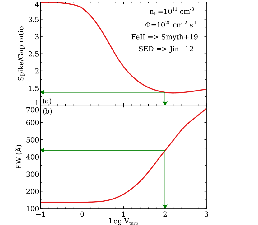
Figure 7: Spike/gap ratio and EW of the Fe ii emission in the UV as a function V_turb. Green line: the Spike/gap ratio and EW of Fe ii UV bump corresponding to V_turb = 100 km/s. These values are consistent with observation. Any turbulence greater than 100 km/s will reproduce the observed Fe ii emission.

3.2 The effects of microturbulence

Figure 8: Similar to Figure 6 except V_turb = 100 km/s. Large regions of parameter space reproduce the observed Spike/Gap ratio $\sim$ 1.4 and EW $>$ 400Å of the $\rm\thinspace I\rm\thinspace ZW\rm\thinspace 1$ in the UV band.

Next we consider clouds with non-zero microturbulent velocity (V_turb) throughout the BLR gas, as previously proposed by Netzer & Wills (1983), and later Bottorff et al. (2000); Baldwin et al. (2004). Netzer & Wills (1983) showed that the strength of the Fe ii UV emission is directly proportional to the microturbulence. The Bottorff et al. (2000), Baldwin et al. (2004), and Bruhweiler & Verner (2008) obtained a better fit for the quasar emission spectra, considering a turbulent emitting cloud. Physically, microturbulence decreases the optical depth by increasing the Doppler broadening ($\tau\sim V_{\rm doppler}^{-1}$), which helps more line photons to escape. Microturbulence also increases the importance of continuum pumping (e.g., Osterbrock, 1977; Phillips, 1978; Ferland, 1992). We present a second grid model by varying V_turb between 0.1 km/s and 10³ km/s. The hydrogen density (n_H) is fixed to 10¹¹ cm^-3 and the photon flux ($\Phi$) to 10²⁰ cm^-2 s^-1, similar to the previous works (e.g., Verner et al., 2003; Véron-Cetty et al., 2004; Baldwin et al., 2004; Bruhweiler & Verner, 2008; Temple et al., 2020). Figure 7 shows the Spike/gap ratio and the strength of Fe ii emission in the UV as a function of V_turb. The Spike/gap ratio decreases with increasing V_turb and attains a value of $\sim$ 1.4 at $V_{\rm turb}\ >60$ km/s. In addition, to reproduce the observed strength of Fe ii emission a V_turb $>$ 90 km/s is needed. Hence we set V_turb = 100 km/s to reproduce the Fe ii spectra for the remainder of the paper.

Next we recalculate the first grid of photoionization models assuming V_turb = 100 km/s to find the n_H and $\Phi$ of the emitting cloud. Similar to the previous steps, we calculate the Spike/gap ratio and the EW of the UV bump for each individual model. Figure 8 presents contour plots of the Spike/gap ratio and EW of the Fe ii UV bump in the n_H–$\Phi$ plane. Clearly, a cloud with n${}_{\rm H}\ \approx\ 10^{11}$ cm^-3 and $\Phi\ \approx\ 10^{20}$ cm^-2 s^-1 reproduces the observed Spike/gap ratio and the strength of Fe ii emission.

Next we compare the Fe ii emission in the UV and optical bands with this density and flux. In Figure 9 we compare the predicted spectra with the observed Fe ii templates in the UV (Vestergaard & Wilkes, 2001) and optical (Véron-Cetty et al., 2004). For further comparison, we include predictions for both thermal and turbulent clouds. The Smyth et al. (2019) dataset, the new-generation SED (Jin et al., 2012), and V_turb = 100 km/s reproduces AGN Fe ii spectra in the UV and optical far better than found in previous work, with solar Fe/H. This is a remarkable accomplishment.

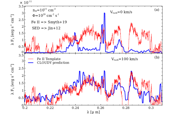
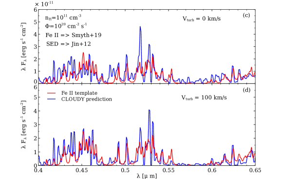
Figure 9: Left: panel (a) shows a comparison between the observed Fe ii UV template (Vestergaard & Wilkes, 2001) and the Cloudy predicted Fe ii UV spectrum with V_turb = 0 km/s. Panel (b) shows the same comparison with V_turb = 100 km/s. Right: panel (c) compares the Fe ii optical template (Véron-Cetty et al., 2004) to the Cloudy predicted spectrum with V_turb = 0 km/s. Panel (d) presents the same comparison except V_turb = 100 km/s. The turbulent model largely reproduces the template.

3.3 Fe ii/Mg ii ratio

The abundances of iron and magnesium are vital to probe the chemical evolution at high redshift. Iron in the solar neighborhood has mostly been produced by Type Ia SNe, which are the last stage of intermediate-mass stars in a close binary system. By comparison, magnesium has been deposited in the ISM by Type II SNe, a core-collapsed SN originating from the explosion of a massive star soon after the initial starburst. Type Ia SNe are delayed compared to Type II SNe. A time lag between the iron and magnesium enrichment of the solar neighborhood is therefore expected. This time delay varies from 0.3 Gyr for massive elliptical galaxies to 1-3 Gyr for Milky-Way type galaxies (Matteucci & Recchi, 2001). Previous observations have measured the $I(\mbox{{\rm Fe~{}{\sc ii}}})/I(\mbox{{\rm Mg~{}{\sc ii}}})$ as a function of look-back time to trace the Fe/Mg abundance ratio (e.g., De Rosa et al., 2011; Shin et al., 2019). More recently Schindler et al. (2020) report on an extensive data set extending over a broad range of cosmic time and find similar $I(\mbox{{\rm Fe~{}{\sc ii}}})/I(\mbox{{\rm Mg~{}{\sc ii}}})$ ratios.

We showed above that our best BLR model with solar abundances could successfully reproduce the observed template of $\rm\thinspace I\rm\thinspace ZW\rm\thinspace 1$ in the UV and optical. To estimate the $I(\mbox{{\rm Fe~{}{\sc ii}}})/I(\mbox{{\rm Mg~{}{\sc ii}}})$, we consider the total flux of the Fe ii UV bump between the 2000Å–3000Å range and that of the Mg ii doublet at 2798Å . We examined the $I(\mbox{{\rm Fe~{}{\sc ii}}})/I(\mbox{{\rm Mg~{}{\sc ii}}})$ for our best-fitting model with n_H = 10¹¹ cm^-3 , $\Phi$ = 10²⁰ cm^-2 s^-1, and V_turb = 100 km/s. Our model predicts log($I(\mbox{{\rm Fe~{}{\sc ii}}})/I(\mbox{{\rm Mg~{}{\sc ii}}})$) $\approx$ 0.7. Shin et al. (2019) obtained log($I(\mbox{{\rm Fe~{}{\sc ii}}})/I(\mbox{{\rm Mg~{}{\sc ii}}})$) values of 0.31 – 0.79 for a large sample of AGNs at $z\ \sim$ 3. De Rosa et al. (2011) showed a maximum log($I(\mbox{{\rm Fe~{}{\sc ii}}})/I(\mbox{{\rm Mg~{}{\sc ii}}})$) of 0.77 for AGNs with $z\ >$ 4. Our log($I(\mbox{{\rm Fe~{}{\sc ii}}})/I(\mbox{{\rm Mg~{}{\sc ii}}})$) predictions closely match those observations, as shown in Figure 11.

Next we vary the Fe abundance from 0.1 to 10 times the solar abundance in our best-fitting BLR model and estimate the $I(\mbox{{\rm Fe~{}{\sc ii}}})/I(\mbox{{\rm Mg~{}{\sc ii}}})$ ratio while keeping the abundances of the other elements constant. This is a test of the sensitivity of the line intensity ratio to the abundance ratio. Figure 10 shows the monotonic increasing nature of the $I(\mbox{{\rm Fe~{}{\sc ii}}})/I(\mbox{{\rm Mg~{}{\sc ii}}})$ ratio as a function of the Fe abundance. A similar trend of the $I(\mbox{{\rm Fe~{}{\sc ii}}})/I(\mbox{{\rm Mg~{}{\sc ii}}})$ ratio with the Fe abundance is also obtained by Verner et al. (2003). The log($I(\mbox{{\rm Fe~{}{\sc ii}}})/I(\mbox{{\rm Mg~{}{\sc ii}}})$) intensity ratio increases by only $\sim 0.4$ dex when the Fe/Mg abundance ratio increases by 2 dex, or $I(\mbox{{\rm Fe~{}{\sc ii}}})/I(\mbox{{\rm Mg~{}{\sc ii}}})$ $\propto$ (Fe/Mg)^0.19. This shows that the Fe ii and Mg ii spectra are strongly saturated due to the large line optical depths so that the intensity ratio does not strongly depend on the abundance ratio. Chemical evolution models suggest that the Fe/Mg ratio jumps by $\sim$ 1 dex when Type Ia supernovae start occurring in giant ellipticals (Hamann & Ferland, 1999). This would correspond to a change in the intensity ratio of log($I(\mbox{{\rm Fe~{}{\sc ii}}})/I(\mbox{{\rm Mg~{}{\sc ii}}})$) $\sim$ 0.19. Clearly a large number of high quality quasar spectra will be needed to measure such a subtle change.

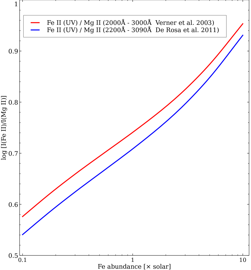
Figure 10: $I(\mbox{{\rm Fe~{}{\sc ii}}})/I(\mbox{{\rm Mg~{}{\sc ii}}})$ as a function of the Fe abundances. We show that the Fe ii/Mg ii ratio for two different UV bands – 2000Å - 3000Å and 2200Å - 3090Å band, as described in Verner et al. (2003) and De Rosa et al. (2011), respectively.

3.4 Eigenvector 1

Next we consider the Eigenvector 1 correlation. The new-generation SED models consider a wide range of L/L_Edd, as summarized by Ferland et al. (2020). We adopt four L/L_Edd values for Jin et al. (2012) SED. Those are log L/L_Edd = $-$1.15, $-$0.55, $-$0.03, and 0.66. Figure 11 shows the predicted change in the equivalent widths of the UV bump and optical emission, defined as the total Fe ii emission integrated over 4000 - 6000Å. Both are predicted as equivalent widths measured relative to the incident SED at 1215Å (Baldwin et al., 2004). The rightmost panel shows the $I(\mbox{{\rm Fe~{}{\sc ii}}})/I(\mbox{{\rm Mg~{}{\sc ii}}})$ discussed above and the ratio of the UV to optical Fe ii bands.

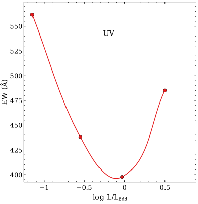
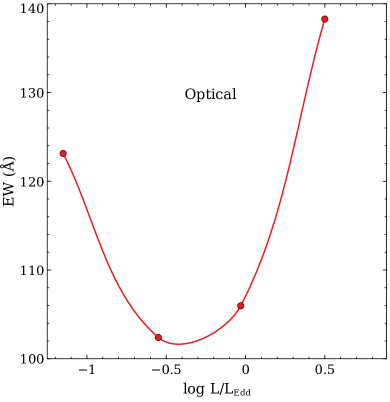
(a)	(b)
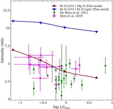
(c)

Figure 11: Panel (a) and (b): red circles show the EW of the Fe ii UV bump and the Fe ii optical band as a function of L/L_Edd respectively. Panel (c): red and blue triangles represent the $I(\mbox{{\rm Fe~{}{\sc ii}}})/I(\mbox{{\rm Mg~{}{\sc ii}}})$ and $I(\mbox{{\rm Fe~{}{\sc ii}}})(\rm UV)/I(\mbox{{\rm Fe~{}{\sc ii}}})(Optical)$ as a function of L/L_Edd, respectively. For both plots we use our best obtained model parameters. Green circles and magenta squares are the observed $I(\mbox{{\rm Fe~{}{\sc ii}}})/I(\mbox{{\rm Mg~{}{\sc ii}}})$ ratios taken from De Rosa et al. (2011) and Shin et al. (2019) respectively.

Although the predictions are in general agreement with observations, the observational scatter makes comparison difficult. De Rosa et al. (2011) and Shin et al. (2019) obtained the $I(\mbox{{\rm Fe~{}{\sc ii}}})/I(\mbox{{\rm Mg~{}{\sc ii}}})$ for AGN samples observed at $z\ >$ 4 and $z\ \sim$ 3, respectively. Their results show little or no correlation between the $I(\mbox{{\rm Fe~{}{\sc ii}}})/I(\mbox{{\rm Mg~{}{\sc ii}}})$ and L/L_Edd. Clearly there are more parameters changing than simply the SED. A similar conclusion was reached by Ferland et al. (2020). That study used analytical theory to predict how the equivalent widths of H i and He ii lines should change with the SED shape. As expected, large increases in the equivalent width were predicted as the SED grew harder with increasing L/L_Edd. No changes in equivalent width are observed, showing that the physics is more complex. Alternatively, the underlying theory may not, for some reason, produce the correct change in the SED as L/L_Edd changes. Clearly more work is needed.

4 Conclusions and Summary

We incorporated four atomic datasets, with self-consistent energy levels, transition rates, and electron impact collision strengths, for Fe ii. Three of these sets include transitions in the UV and we compared the emission line predictions from these datasets for typical AGN with a set of BLR parameters and the new generation of SEDs.

• The original Verner et al. (1999) dataset largely rests on “g-bar” collision strengths, so we only presented it as a reference. By contrast, the Tayal & Zatsarinny (2018) and Smyth et al. (2019) Fe ii datasets have many more transitions in the FUV, so continuum and Ly$\alpha$ florescent excitation, known to be important for Fe ii, is better reproduced. However, the Smyth et al. (2019) dataset, with its higher density of states, produces several times more emission in the FUV compared to Tayal & Zatsarinny (2018). The Smyth et al. (2019) dataset was hence adopted throughout most of this work.

• We considered three representations of the broadband SED of an AGN, namely the original Mathews & Ferland (1987) SED (long included in Cloudy), the Korista et al. (1997) SED derived from observations, and that of Jin et al. (2012) SED derived from a combination of theory and more recent observations. We compared the Fe ii emission lines reproduced by each of the SEDs with Cloudy. We showed that the Jin et al. (2012) SED produces the strongest Fe ii emission because the soft X-rays penetrate into the low ionization region, heating it, generating more Fe ii emission. Also, the log L/L_Edd value for the intermediate Jin et al. (2012) SED is consistent with that of $\rm\thinspace I\rm\thinspace ZW\rm\thinspace 1$. The Jin et al. (2012) SED was hence adopted in this work.

• We presented predictions of the strength of the broad bump of Fe ii UV emission and the Spike/gap ratio, defined by Baldwin et al. (2004), in the density (n_H) – photon flux ($\Phi$) plane, using solar abundances and thermal line broadening (V_turb = 0 km/s). Our calculations with the Smyth et al. (2019) dataset and the Jin et al. (2012) SED also did not reproduce the observed Fe ii template.

• We considered the effects of microturbulence (V_turb), varying it between 10^-1–10³ km/s. We showed that a cloud with V_turb $>$ 60 km/s closely reproduces the observed Spike/gap ratio of 1.4, while the observed equivalent width ($>$ 400 Å) requires that V_turb $>$ 90 km/s. We adopted V_turb $\approx$ 100 km/s in this work.

• Using the Smyth et al. (2019) dataset, Jin et al. (2012) SED, solar abundances, and the derived V_turb, we recalculated the strength of the Fe ii UV emission and Spike/gap ratio in the density (n_H) – photon flux ($\Phi$) plane. We showed that large regions in the plane reproduced the observed UV Fe ii emission.

• We compared our model using the best obtained BLR parameters with the observed Fe ii UV (Vestergaard & Wilkes, 2001) and optical template Véron-Cetty et al. (2004) template and found surprisingly good agreement. We concluded that the Fe ii spectra are consistent with formation in relatively dense (n${}_{\rm H}=10^{11}$ cm^-3) and turbulent (V_turb $\approx$ 100 km/s) clouds about 100 – 200 light days away from the central black hole with solar abundances.

• We showed that the $I(\mbox{{\rm Fe~{}{\sc ii}}})/I(\mbox{{\rm Mg~{}{\sc ii}}})$ ratio predicted by our best-fitting model reproduces observations with solar abundances. This is a significant step in calibrating Fe ii as an abundance indicator. Unfortunately, the spectrum is strongly saturated so the intensity ratio does not have a strong dependence on the abundance ratio.

• We considered how changes in the SED shape, predicted from recent models by varying L/L_Edd, change the resultant Fe ii spectrum. In the simplest case this would provide a physical explanation for the observed Eigenvector 1 relations. The predicted changes do not agree with the observed correlations, showing that more is changing than just the SED shape. A similar conclusion was reached by Ferland et al. (2020) in their analysis of hydrogen line equivalent widths.

References

- Allende Prieto et al. (2002) Allende Prieto, C., Lambert, D. L., & Asplund, M. 2002, ApJ, 573, L137, doi: 10.1086/342095
- Baldwin et al. (1995) Baldwin, J., Ferland, G., Korista, K., & Verner, D. 1995, ApJ, 455, L119, doi: 10.1086/309827
- Baldwin et al. (2004) Baldwin, J. A., Ferland, G. J., Korista, K. T., Hamann, F., & LaCluyzé, A. 2004, ApJ, 615, 610, doi: 10.1086/424683
- Bautista et al. (2015) Bautista, M. A., Fivet, V., Ballance, C., et al. 2015, ApJ, 808, 174, doi: 10.1088/0004-637X/808/2/174
- Bolton & Haehnelt (2007) Bolton, J. S., & Haehnelt, M. G. 2007, MNRAS, 374, 493, doi: 10.1111/j.1365-2966.2006.11176.x
- Boroson & Green (1992) Boroson, T. A., & Green, R. F. 1992, ApJS, 80, 109, doi: 10.1086/191661
- Bottorff et al. (2000) Bottorff, M., Ferland, G., Baldwin, J., & Korista, K. 2000, The Astrophysical Journal, 542, 644, doi: 10.1086/317051
- Bruhweiler & Verner (2008) Bruhweiler, F., & Verner, E. 2008, ApJ, 675, 83, doi: 10.1086/525557
- Bruhweiler & Verner (2008) Bruhweiler, F., & Verner, E. 2008, The Astrophysical Journal, 675, 83, doi: 10.1086/525557
- Cracco et al. (2016) Cracco, V., Ciroi, S., Berton, M., et al. 2016, MNRAS, 462, 1256, doi: 10.1093/mnras/stw1689
- De Rosa et al. (2011) De Rosa, G., Decarli, R., Walter, F., et al. 2011, ApJ, 739, 56, doi: 10.1088/0004-637X/739/2/56
- Djorgovski et al. (2001) Djorgovski, S. G., Castro, S., Stern, D., & Mahabal, A. A. 2001, ApJ, 560, L5, doi: 10.1086/324175
- Done et al. (2012) Done, C., Davis, S. W., Jin, C., Blaes, O., & Ward, M. 2012, MNRAS, 420, 1848, doi: 10.1111/j.1365-2966.2011.19779.x
- Fan et al. (2006) Fan, X., Carilli, C. L., & Keating, B. 2006, ARA&A, 44, 415, doi: 10.1146/annurev.astro.44.051905.092514
- Ferland (1992) Ferland, G. J. 1992, ApJ, 389, L63, doi: 10.1086/186349
- Ferland et al. (2020) Ferland, G. J., Done, C., Jin, C., Landt, H., & Ward, M. J. 2020, MNRAS, 494, 5917, doi: 10.1093/mnras/staa1207
- Ferland et al. (2009) Ferland, G. J., Hu, C., Wang, J.-M., et al. 2009, ApJ, 707, L82, doi: 10.1088/0004-637X/707/1/L82
- Ferland et al. (2017) Ferland, G. J., Chatzikos, M., Guzmán, F., et al. 2017, Rev. Mexicana Astron. Astrofis., 53, 385. https://arxiv.org/abs/1705.10877
- Garcia-Rissmann et al. (2012) Garcia-Rissmann, A., Rodríguez-Ardila, A., Sigut, T. A. A., & Pradhan, A. K. 2012, ApJ, 751, 7, doi: 10.1088/0004-637X/751/1/7
- Giustini & Proga (2019) Giustini, M., & Proga, D. 2019, A&A, 630, A94, doi: 10.1051/0004-6361/201833810
- Grevesse & Sauval (1998) Grevesse, N., & Sauval, A. J. 1998, Space Sci. Rev., 85, 161, doi: 10.1023/A:1005161325181
- Hamann & Ferland (1999) Hamann, F., & Ferland, G. 1999, ARA&A, 37, 487, doi: 10.1146/annurev.astro.37.1.487
- Holweger (2001) Holweger, H. 2001, in American Institute of Physics Conference Series, Vol. 598, Joint SOHO/ACE workshop “Solar and Galactic Composition”, ed. R. F. Wimmer-Schweingruber, 23–30, doi: 10.1063/1.1433974
- Jin et al. (2012) Jin, C., Ward, M., & Done, C. 2012, MNRAS, 425, 907, doi: 10.1111/j.1365-2966.2012.21272.x
- Kim et al. (2009) Kim, S., Stiavelli, M., Trenti, M., et al. 2009, ApJ, 695, 809, doi: 10.1088/0004-637X/695/2/809
- Korista et al. (1997) Korista, K., Baldwin, J., Ferland, G., & Verner, D. 1997, ApJS, 108, 401, doi: 10.1086/312966
- Kovačević-Dojčinović & Popović (2015) Kovačević-Dojčinović, J., & Popović, L. Č. 2015, ApJS, 221, 35, doi: 10.1088/0067-0049/221/2/35
- Kurk et al. (2007) Kurk, J. D., Walter, F., Fan, X., et al. 2007, ApJ, 669, 32, doi: 10.1086/521596
- Kwan & Krolik (1981) Kwan, J., & Krolik, J. H. 1981, ApJ, 250, 478, doi: 10.1086/159395
- Leighly et al. (2007) Leighly, K. M., Halpern, J. P., Jenkins, E. B., & Casebeer, D. 2007, ApJS, 173, 1, doi: 10.1086/519768
- Marinucci et al. (2018) Marinucci, A., Bianchi, S., Braito, V., et al. 2018, MNRAS, 478, 5638, doi: 10.1093/mnras/sty1436
- Marziani & Sulentic (2014) Marziani, P., & Sulentic, J. W. 2014, Advances in Space Research, 54, 1331, doi: 10.1016/j.asr.2013.10.007
- Marziani et al. (2001) Marziani, P., Sulentic, J. W., Zwitter, T., Dultzin-Hacyan, D., & Calvani, M. 2001, ApJ, 558, 553, doi: 10.1086/322286
- Mathews & Ferland (1987) Mathews, W. G., & Ferland, G. J. 1987, ApJ, 323, 456, doi: 10.1086/165843
- Matteucci & Recchi (2001) Matteucci, F., & Recchi, S. 2001, ApJ, 558, 351, doi: 10.1086/322472
- Mazzucchelli et al. (2017) Mazzucchelli, C., Bañados, E., Venemans, B. P., et al. 2017, ApJ, 849, 91, doi: 10.3847/1538-4357/aa9185
- Netzer (2020) Netzer, H. 2020, MNRAS, 494, 1611, doi: 10.1093/mnras/staa767
- Netzer & Wills (1983) Netzer, H., & Wills, B. J. 1983, ApJ, 275, 445, doi: 10.1086/161545
- Osterbrock (1977) Osterbrock, D. E. 1977, ApJ, 215, 733, doi: 10.1086/155407
- Panda et al. (2018) Panda, S., Czerny, B., Adhikari, T. P., et al. 2018, ApJ, 866, 115, doi: 10.3847/1538-4357/aae209
- Panda et al. (2019) Panda, S., Marziani, P., & Czerny, B. 2019, ApJ, 882, 79, doi: 10.3847/1538-4357/ab3292
- Peterson (1993) Peterson, B. M. 1993, PASP, 105, 247, doi: 10.1086/133140
- Phillips (1978) Phillips, M. M. 1978, ApJS, 38, 187, doi: 10.1086/190553
- Ruff et al. (2012) Ruff, A. J., Floyd, D. J. E., Korista, K. T., et al. 2012, in Journal of Physics Conference Series, Vol. 372, Journal of Physics Conference Series, 012069, doi: 10.1088/1742-6596/372/1/012069
- Sarkar & Samui (2019) Sarkar, A., & Samui, S. 2019, PASP, 131, 074101, doi: 10.1088/1538-3873/ab10ea
- Schindler et al. (2020) Schindler, J.-T., Farina, E. P., Banados, E., et al. 2020, arXiv e-prints, arXiv:2010.06902. https://arxiv.org/abs/2010.06902
- Shen & Ho (2014) Shen, Y., & Ho, L. C. 2014, Nature, 513, 210, doi: 10.1038/nature13712
- Shin et al. (2019) Shin, J., Nagao, T., Woo, J.-H., & Le, H. A. N. 2019, ApJ, 874, 22, doi: 10.3847/1538-4357/ab05da
- Smyth et al. (2019) Smyth, R. T., Ramsbottom, C. A., Keenan, F. P., Ferland , G. J., & Ballance, C. P. 2019, MNRAS, 483, 654, doi: 10.1093/mnras/sty3198
- Sulentic et al. (2000) Sulentic, J. W., Zwitter, T., Marziani, P., & Dultzin-Hacyan, D. 2000, ApJ, 536, L5, doi: 10.1086/312717
- Tayal & Zatsarinny (2018) Tayal, S. S., & Zatsarinny, O. 2018, Phys. Rev. A, 98, 012706, doi: 10.1103/PhysRevA.98.012706
- Temple et al. (2020) Temple, M. J., Ferland, G. J., Rankine, A. L., et al. 2020, MNRAS, 496, 2565, doi: 10.1093/mnras/staa1717
- Verner et al. (2003) Verner, E., Bruhweiler, F., Verner, D., Johansson, S., & Gull, T. 2003, ApJ, 592, L59, doi: 10.1086/377571
- Verner et al. (1999) Verner, E. M., Verner, D. A., Korista, K. T., et al. 1999, ApJS, 120, 101, doi: 10.1086/313171
- Véron-Cetty et al. (2004) Véron-Cetty, M. P., Joly, M., & Véron, P. 2004, A&A, 417, 515, doi: 10.1051/0004-6361:20035714
- Vestergaard & Wilkes (2001) Vestergaard, M., & Wilkes, B. J. 2001, ApJS, 134, 1, doi: 10.1086/320357
- Wang et al. (2016) Wang, T., Ferland, G. J., Yang, C., Wang, H., & Zhang, S. 2016, ApJ, 824, 106, doi: 10.3847/0004-637X/824/2/106
- Wills et al. (1985) Wills, B. J., Netzer, H., & Wills, D. 1985, ApJ, 288, 94, doi: 10.1086/162767
- Wu et al. (2015) Wu, X.-B., Wang, F., Fan, X., et al. 2015, Nature, 518, 512, doi: 10.1038/nature14241