Multiphase tin equation of state using density functional theory

Abstract

We perform density functional theory (DFT) calculations of five solid phases and the liquid phase of tin. The calculations include cold curves of the five solid phases, phonon calculations in the quasi-harmonic approximation over a range of volumes for each solid phase, and DFT-based molecular dynamics (DFT-MD) calculations of the liquid phase. Using the DFT results, we construct a tabular multiphase SESAME equation of state for tin, referred to as SESAME 2162. Comparisons to experimental data are made and show a high level of agreement in isobaric data, isothermal data, shock data, and phase boundary measurements, including measurements of the melt curve. The 2162 EOS will be useful for hydrodynamics simulations and has been designed with an eye toward hydrodynamics simulations that incorporate materials strength models and allow for modeling of the kinetics of phase transitions.

I Introduction

Tabular equations of state (EOS) are important for both a basic understanding of materials properties and for hydrodynamics applications. As hydrodynamics codes are developed to incorporate materials strength models Preston et al. (2003); Barton et al. (2011) and to account for kinetic effects in simulating phase transitions,Greeff (2016); Andrews (1971); Wills et al. (2016) the need for an accurate underlying multiphase EOS becomes increasingly important. Here we focus on the development of a new tabular multiphase SESAME Lyon (1992); Chisolm et al. (2005a) EOS for tin, referred to as SESAME 2162. The EOS can be thought of as a successor to the previous tin EOS, SESAME 2161. Greeff et al. (2005) The new EOS includes four solid phases and the liquid phase.

To generate SESAME 2162, we performed density functional theory (DFT) calculations of the solid phases of tin and the liquid phase, including static lattice energy (cold curve) calculations, phonon calculations in the quasi-harmonic approximation, and DFT-based molecular dynamics (DFT-MD) calculations of the liquid phase, including calculations of the melt curve. These calculations provide data in regions of the state space where experimental data is unavailable and thereby help to constrain construction of the final EOS.

Tin is known to exist in at least 5 different solid phases, summarized in Table 1. Throughout, we refer to the phases by their corresponding Greek letter. Note that the $\alpha$, $\beta$, and $\gamma$ naming conventions are all standard. Here we also use $\delta$ to refer to the bcc phase, which has infrequently been referred to as the $\sigma$ phase in the past, Molodets and Nabatov (2000) and we use $\epsilon$ to refer to the hcp phase. The Greek letters are chosen in ascending order according to the pressure at which each phase becomes stable.

Although we performed DFT calculations for all five solid phases, we include only the $\beta$, $\gamma$, $\delta$, and $\epsilon$ phases in the 2162 EOS, since the $\alpha$ phase is only stable below room temperature and at pressures below 1 GPa Young (1991); Tonkov and Ponyatovsky (2018); Nikolaev et al. (1973) with limited accessibility in compressive and shock experiments, which are the main focus of hydrodynamics codes that use the EOS. In addition, the transition from $\beta\rightarrow\alpha$ is slow and therefore unlikely to show up in experiments. Anderson et al. (2000); Cornelius et al. (2017)

phase	lattice type	space group	space group #	# atoms/cell
$\alpha$	diamond	$Fd\bar{3}m$	227	2
$\beta$	bct	$I4_{1}/amd$	141	4
$\gamma$	bct	$I4/mmm$	139	2
$\delta$	bcc	$Im\bar{3}m$	229	1
$\epsilon$	hcp	$P6_{3}/mmc$	194	2

Table 1: Summary of the crystal structures and space groups of the 5 known solid phases of tin. Greek letters are used to refer to the phases in ascending order, from low to high pressure. DFT calculations are performed using a mixture of primitive and conventional unit cells, with the number of atoms per cell indicated in the last column.

Many experiments have been performed on tin, including isobaric measurements, Kammer et al. (1972); Touloukian (1975); Swanson (1953); Alchagirov and Chochaeva (2000); Wang et al. (2003); Hultgren et al. (1973); Thewlis and Davey (1954); Prasad and Wooster (1955) isothermal diamond anvil cell (DAC) measurements, Olijnyk and Holzapfel (1984); Liu and Liu (1986); Desgreniers et al. (1989); Plymate et al. (1988); Cavaleri et al. (1988); Salamat et al. (2011, 2013); Stager et al. (1962); Barnett et al. (1966); Vaidya and Kennedy (1970) shock experiments, Walsh et al. (1957); Al’tshuler et al. (1958); McQueen and Marsh (1960); Al’Tshuler et al. (1962); Marsh (1980); Al’Tshuler et al. (1981); Hu et al. (2008); Rice et al. (1958) dynamic compression experiments, Lazicki et al. (2015) and measurements of the solid-solid phase boundaries. Kingon et al. (1980); Xu et al. (2014); Barnett et al. (1963); Hinton et al. (2020) Measurements of the phonon dispersions for the $\alpha$, $\beta$, and $\gamma$ phases have been also been made. Price et al. (1971); Rowe (1967); Ivanov et al. (1987, 1995); Giefers et al. (2007) In addition, the melt curve has been measured in a variety of different ways, including shock-induced melt Mabire and Hereil (2000a, b); Seagle et al. (2013); Briggs et al. (2019); Héreil and Mabire (2002) and resistive and/or laser heating in a DAC or compressive piston. Dudley and Hall (1960); Weir et al. (2012); La Lone et al. (2019); Jayaraman et al. (1963); Narushima et al. (2007); Briggs et al. (2012, 2017); Schwager et al. (2010) The available melt curve data show a large variability in the range of measurements. More recently, studies on liquid spallation and fragmentation have also been performed. De Rességuier et al. (2007); Signor et al. (2010); Anderson et al. (2000) In addition, a wide range of theoretical calculations of tin have been performed, including DFT-based cold curve calculations, Corkill et al. (1991); Hafner (1974); Ihm and Cohen (1981); Cheong and Chang (1991); Christensen (1993); Christensen and Methfessel (1993); Aguado (2003); Yu et al. (2006); Cui et al. (2008); Yao and Klug (2011) phonon calculations, Wehinger et al. (2014); Rowe et al. (1965); Chen (1967); Pavone et al. (1998) and molecular dynamics calculations, Bernard and Maillet (2002); Zhang et al. (2011); Ravelo and Baskes (1997); Soulard and Durand (2020) and a variety of equations of state for tin have been proposed over the years. Greeff et al. (2005); Buy et al. (2006); Cox (2006); Khishchenko (2008); Cox and Christie (2015)

The rest of the paper is organized as follows: in Sec. II, we provide an overview of OpenSesame, the program used to generate SESAME 2162. In Sec. III we provide details on the calculations of the cold curves and phonon calculations of the solid phases, and of the DFT-MD calculations of the liquid phase. We also describe how these calculations are used to determine an initial set of parameters for models used in OpenSesame to construct the 2162 EOS. In Sec. IV, we discuss how the parameters from DFT are modified (when necessary) to obtain agreement with experimental data and create the 2162 EOS. We show comparisons of the 2162 EOS to a variety of experimental measurements, including isobaric data, isothermal DAC data, shock data, solid-solid phase boundary measurements, and measurements of the melt curve. While we only summarize the main results here, a more comprehensive description of the process used to incorporate DFT calculations into materials models used in OpenSesame, as well as a more detailed description of how model parameters are adjusted to fit to experimental data, is provided in Ref. Rehn et al., a.

II Overview of OpenSesame

The OpenSesame software is a useful tool for generating tabular materials equations of state. The multiphase capability in OpenSesame Chisolm et al. (2005a) relies on individual phase EOS tables and evaluates the phase with the lowest Gibbs free energy at a given temperature and pressure. Mixed phases are handled in a self-consistent manner, as described below. The multiphase capability allows for an arbitrary number of materials phases to be included in the final EOS table. For the individual phase tables, OpenSesame uses a decomposition of the total Helmholtz free energy $F(V,T)$ for each phase into three pieces,

$$F(V,T)=F_{\mathrm{cold}}(V)+F_{\mathrm{ion}}(V,T)+F_{\mathrm{el}}(V,T),$$ (1)

where $F_{\mathrm{cold}}$ is the energy associated with a cold curve ($T=0$ static lattice energy), $F_{\mathrm{ion}}$ is the free energy associated with ionic motion, and $F_{\mathrm{el}}$ is the electronic free energy. OpenSesame uses a variety of simple materials models to inform on these three contributions to the free energy, making it necessary to determine model parameters from the DFT calculations and/or experimental data. In constructing the 2162 EOS, we first determined model parameters entirely from DFT calculations, as discussed in Sec. III. Because the DFT calculations resulted in an EOS that was not in perfect agreement with experimental data, small modifications to the model parameters were made, as described in Sec. IV.

Model parameters for the solid phases determined by DFT are outlined in Sec. III. In Sec. III.1, we discuss cold curve calculations that inform directly on $F_{\mathrm{cold}}$, which we treat with a Vinet-Rose model. Vinet et al. (1987) In Sec. III.2, we show how phonon calculations can be used to determine parameters in the Debye model Debye , which informs on $F_{\mathrm{ion}}$ for the solid phases. The Debye model relies on the Debye frequency $\nu_{D}$, or equivalently the Debye temperature $\Theta_{D}=h\nu_{D}/k_{B}$. Also necessary for $F_{\mathrm{ion}}$ is a Grüneisen model, also discussed in Sec. III.2, that provides information about the volume dependence of the Debye frequencies. DFT-based phonon calculations allow for the determination of all parameters relevant to the Debye and Grüneisen models for the solid phases. The remaining term $F_{\mathrm{el}}$ is determined using the Thomas-Fermi-Dirac (TFD) method Chisolm (2003); Thomas (1927); Fermi (1927); Dirac (1930) and does not require additional parameterization from DFT calculations.

For the liquid phase, the same decomposition in Eq. 1 is used. The liquid free energy is defined with respect to that of a reference solid phase, which we denote $F_{\rm rs}$. This may be one of the actual solid phases, or may be hypothetical. We define a scaling temperatature $T_{\rm sc}(V)$, which marks the transition from solid-like to liquid-like behavior. For $T\leq T_{\rm sc}$, the liquid free energy $F_{\rm l}$ is related to that of the reference solid by a constant entropy shift $\Delta S$ and a volume-dependent energy shift $\Delta F_{\rm cold}(V)$,

$$F_{\rm l}(V,T)=F_{\rm rs}(V,T)-\Delta ST+\Delta F_{\rm cold}(V);\,\,\,T\leq T_{\rm sc}(V),$$ (2)

where $F_{\rm rs}$ is parameterized the same way as the other solid phases. For $T>T_{\rm sc}(V)$ the excess specific heat is assumed to be a function of the scaled temperature

$$c_{V}(V,T)/Nk_{B}=f(T/T_{\rm sc}(V))+3/2\,,$$ (3)

with $f(1)=3/2$ and $f(x)\rightarrow 0$ as $x\rightarrow\infty$. Eqs. 2 and 3 allow one to determine the free energy at all temperatures,

$$F_{\rm l}(V,T)= F_{\rm l}(V,T_{\rm sc}(V))-S_{\rm l}(V,T_{\rm sc}(V))(T-T_{\rm sc}(V))$$

$$-\int_{T_{\rm sc}}^{T}\mathrm{d}T_{2}\int_{T_{\rm sc}}^{T_{2}}\mathrm{d}T_{1}\frac{c_{V}(V,T_{1})}{T_{1}};\,\,\,T>T_{\rm sc}(V)$$ (4)

The details of the $T$-dependence of $c_{V}$ are described in Ref. Chisolm et al., 2005b. We define $T_{\rm m}(V)=\Delta F_{\rm cold}(V)/\Delta S$. Then the volume dependence of the two functions $T_{\rm sc}(V)$ and $T_{\rm m}(V)$ is given by

$$-{\mathrm{d}\ln T_{\rm m}(V)\over\mathrm{d}\ln V} = 2\Gamma_{\rm m}(V)-2/3$$ (5)

$$-{\mathrm{d}\ln T_{\rm sc}(V)\over\mathrm{d}\ln V} = 2\Gamma_{\rm rs}(V)-2/3$$ (6)

where the Grüneisen parameters $\Gamma_{\rm m}$ and $\Gamma_{\rm rs}$ have the same functional form as those of the solid phase Debye temperatures, as given in Eq. 11, discussed in the next section. Note that the effective Grüneisen parameter for $T_{\rm sc}$ as defined in Eq. 6 must be the same as the Debye Grüneisen parameter for the reference solid, $\Gamma_{\rm rs}=-\mathrm{d}\ln\theta_{\rm rs}/\mathrm{d}\ln V$, in order for the pressure to reach the ideal gas limit at high temperature.Grover (1971)

The liquid free energy has, in addition to the standard solid phase parameters, two additional parameters for the volume dependence of $\Gamma_{\rm m}$, as well as $\Delta S$ and reference values for $T_{\rm m}$ and $T_{\rm sc}$. This somewhat complicated formulation was adopted to facilitate creating liquid models that obey standard Lindemann scaling Grover (1971) in the case of a single solid phase. For that case, the reference solid is the actual solid phase, the various Grüneisen parameters are the same, and the reference values of $T_{\rm m}$ and $T_{\rm sc}$ are the same and are equal to the melting temperature at the reference volume. The earlier SESAME 2161 tin EOS was made with the liquid “normal” in this sense with respect to the high pressure $\gamma$ phase. For SESAME 2162, there are more solid phases, we have more data on the high pressure melting curve, as well as DFT-MD data on the liquid EOS, and thus were not able to adopt this simplification. When developing the 2162 EOS, we explored three options for determining a cold curve for the liquid, as described in Ref. Rehn et al., a. Because melt is possible from the $\beta$, $\gamma$, and $\delta$ phases of tin across a wide compression range, we determined a cold curve that interpolates across the three solid phases, also described in Ref. Rehn et al., a.

In the construction of SESAME 2162, we produce an equilibrium table that includes mixed phase regions. The mixed phase regions are defined by the following set of equations,

$$P_{a}(V_{a},T) = P_{b}(V_{b},T)$$

$$G_{a}(V_{a},T) = G_{b}(V_{b},T)$$

$$\lambda_{a}V_{a}+\lambda_{b}V_{b} = V$$

$$\lambda_{a}E_{a}(V_{a},T)+\lambda_{b}E_{b}(V_{b},T) = E$$ (7)

where $a$ and $b$ denote the two coexisting phases, $P$, $G$, $V$, and $E$ are the pressure, specific Gibbs free energy, volume, and internal energy, respectively, and $\lambda_{a}$ denotes the mass fraction of phase $a$. For the great majority of states, there are no solutions to the conditions (Eqs. 7) satisfying $0\leq\lambda_{i}\leq 1$ and $\sum_{i}\lambda_{i}=1$, and the state is a pure phase with the lowest Helmholtz free energy at the given $V$ and $T$. The algorithm for constructing equilibrium tables is described in Ref. Chisolm et al., 2005a.

The initial set of model parameters determined from DFT calculations provide a useful starting point for the determination of the OpenSesame model parameters described above. However, some adjustments are needed to agree fully with experimental data. The adjustments made are described in Sec. IV.

III DFT Calculations

III.1 Cold curves

All DFT calculations were computed using the Vienna ab-initio Simulation Package (VASP), Kresse and Hafner (1993, 1994); Kresse and Furthmüller (1996a, b) version 5.4.4. All calculations use the projector augmented wave (PAW) method Blöchl (1994); Kresse and Joubert (1999) using either 14 valence states, 4d¹⁰5s²5p² (cold curves and phonons) or 4 valence states, 5s²5p² (DFT-MD of the liquid). The cold curves were computed by relaxing the structures with multiple restarts to ensure convergence of the atomic positions and lattice constants. The relaxations were performed using the Methfessel-Paxton scheme Methfessel and Paxton (1989) with a 400 eV plane-wave energy cutoff. Subsequently, total energy calculations were performed using fixed ions and lattice constants with tetrahedral integration of the Brillouin zone and a 520 eV plane-wave energy cutoff. We also computed cold curves of tin using the all-electron code RSPt Wills et al. (2010) with different relativistic treatments Rehn et al. (2020, b) and found the results to be in close agreement with the VASP results, indicating the adequacy of using PAW method for treatment of the core states.

Cold curves were computed using the AM05 Armiento and Mattsson (2005) and PBE Perdew et al. (1996) exchange-correlation functionals. As shown in Fig. 1, the AM05 results for the $\beta$ and $\gamma$ phases are in very close agreement with experimental room temperature DAC measurements from Refs. Olijnyk and Holzapfel, 1984; Liu and Liu, 1986; Desgreniers et al., 1989 (note that the phase transition from $\beta$ to $\gamma$ occurs at approximately 8.5 g/cm³), whereas the equilibrium density $\rho_{0}$ predicted by PBE is substantially lower. For this reason, we chose to use the AM05 functional to determine the initial set of 2162 model parameters, which include the AM05 cold curves, AM05 phonon calculations, and DFT-MD calculations using AM05. The only exception to this are DFT-MD calculations of the melt curve using the $Z$ method Belonoshko et al. (2006); Burakovsky et al. (2014, 2015), which were computed separately using the PBE functional. Burakovsky . We present the melt curves only in $P$-$T$ space (see Fig. 4). These results should be expected to be quite similar to what would be obtained using the AM05 functional, since the primary difference between AM05 and PBE is an offset in the density, while the pressure as a function of the compression $\rho/\rho_{0}$ for the two functionals are quite similar, as can be seen in Fig. 1 and as verified by highly similar bulk moduli computed from the cold curves (see Ref. Rehn et al., a for details).

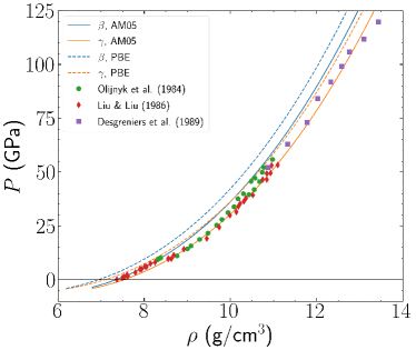
Figure 1: Cold curves for the $\beta$ (blue) and $\gamma$ (orange) phases of tin using the AM05 (solid lines) and PBE (dashed lines) exchange-correlation functionals. Experimental DAC data are from Refs. Olijnyk and Holzapfel, 1984; Liu and Liu, 1986; Desgreniers et al., 1989.

The Vinet-Rose cold curve model was used to fit to the AM05 data of each phase. The results for $\rho_{0},E_{0},B$, and $B^{\prime}=dB/dP$ are provided in Table 2. Note that for cold curve calculations of the $\beta$, $\gamma$, and $\epsilon$ phases, the lattice constants are allowed to relax at each volume to allow for a volume-dependent $c/a$ ratio. In the case of the $\beta$ and $\epsilon$ phases, $c/a$ remains relatively constant over the full compression ranged studied, varying by only a few percent across a compression range of approximately 0.9 to 3.0. On the other hand, the $\gamma$ phase shows a large variation in the $c/a$ ratio, starting at $c/a=0.88$ at $\rho_{0}=7.53$ g/cm³ and converging to $c/a=1$ above 9.38 g/cm³, thereby indicating that the bcc $\delta$ phase has the lower energy above a compression ratio of approximately 1.25. The $\gamma$-$\delta$ phase transition is observed to occur between 10.5–11 g/cm³ (compression of approximately 1.4–1.45) in recent isothermal DAC measurements, Salamat et al. (2013) which is in agreement with the compression range at which the enthalpies of the $\gamma$ and $\delta$ phases computed using the AM05 cold curves cross. Additional details regarding cold curve comparisons and the enthalpy are provided in Ref. Rehn et al., a, and comparisons of the room temperature 2162 isotherms to experimental DAC data are provided in Sec. IV.

We also point out that at non-zero temperatures, the electronic free energy $F_{\mathrm{el}}$ can be determined through the use of Fermi smearing in DFT calculations. This is analogous to cold curve calculations, but with the Fermi smearing width set according to the temperature $k_{B}T$. Although this can provide useful information, we did not see any appreciable differences in the resulting phase boundaries when including Fermi smearing to treat the electronic free energy at a range of temperatures and volumes. In OpenSesame, the electronic free energy is treated with the TFD model, Chisolm (2003); Thomas (1927); Fermi (1927); Dirac (1930) which works over a wide range of densities and temperatures. Similar to the use of Fermi smearing, the TFD method results in only small quantitative differences in the resulting solid-solid phase boundaries, thereby indicating that the TFD method can safely be used for the solid phases of tin.

III.2 Phonons

phase	$\rho_{0}$ (g/cm3)	$E_{0}$ (J/g)	$B$ (GPa)	$B^{\prime}$	$\Theta_{D}$ (K)	$\Gamma_{\mathrm{ref}}$	$\Gamma^{\prime}_{\mathrm{ref}}$
$\beta$	7.336 (7.4375)	0	52.74 (58.0)	5.369	161.0	1.98 (2.42)	-1.31
$\gamma$	7.525	6.04 (36.0)	52.32	5.344	121.7	2.48 (2.45)	-1.82 (-2.20)
$\delta$	7.561	12.55 (54.0)	52.64	5.383	114.2 (117.5)	2.54 (2.51)	-1.73 (-2.10)
$\epsilon$	7.531	3.05 (44.1)	52.68	5.291	121.1 (124.6)	2.51 (2.48)	-1.85 (-2.24)
liquid	(7.470)	(24.0)	(52.7)	(5.540)	(131.0)	(2.45)	(-3.50)

Table 2: Model parameters used to construct the 2162 EOS. The DFT-calculated values using the AM05 functional are displayed first. If modifications were made to the parameter to better agree with experimental data, the final value used in the 2162 EOS is listed in parentheses next to the DFT-calculated value. Note that $\Theta_{D}$, $\Gamma_{\mathrm{ref}}$, and $\Gamma^{\prime}_{\mathrm{ref}}$ for each phase are calculated at a reference density chosen to be $\rho_{\mathrm{ref}}=7.581$ g/cm³ for all phases. All liquid parameters are listed in parentheses because there is not a unique way to determine the values strictly from DFT calculations. The values chosen are ones that were found to best agree simultaneously with the DFT-MD data in Fig. 4 and Hugoniot data in the liquid phase in Fig. 8. Also note that we use the liquid-specific reference parameters $T_{\rm m}=T_{\rm sc}=580$ K, $\Gamma_{\rm m}=\Gamma_{\rm rs}=2.45$, and $\Delta S=0.9$ kJ/g/K.

Phonon calculations were performed in the quasi-harmonic approximation Dove (1993) using a frozen phonon supercell approach in VASP. The Phonopy Togo and Tanaka (2015) package was used to generate supercells and atomic displacements for each solid phase. The plane-wave energy cutoff, k-mesh size, and supercell size were tested at the AM05-predicted equilibrium volume for each phase individually to ensure structural stability of each phase and to ensure a converged phonon density of states. We use a minimum 350 eV plane-wave energy cutoff for each solid phase and used the method of Methfessel and Paxton Methfessel and Paxton (1989) to sample the Brillouin zone. In all calculations we determine the k-mesh of the Brillouin zone using a $\Gamma$-centered Monkhorst-Pack Monkhorst and Pack (1976) scheme. The supercells were constructed using the primitive or conventional cells listed in Table 1, including a 54 atom cell with a $6\times 6\times 6$ k-mesh ($\alpha$ phase), a 64 atom cell with an $8\times 8\times 6$ k-mesh ($\beta$ phase), a 54 atom cell with an $8\times 8\times 8$ k-mesh ($\gamma$ phase), a 64 atom cell with a $6\times 6\times 6$ k-mesh ($\delta$ phase), and a 54 atom cell with a $10\times 10\times 7$ k-mesh ($\epsilon$ phase). At volumes below the equilibrium volume, we use the same k-mesh size to ensure that results remain converged with respect to k-mesh size. The phonon densities of states $g(\nu)$ for each phase at their respective equilibrium volumes are shown in Fig. 2.

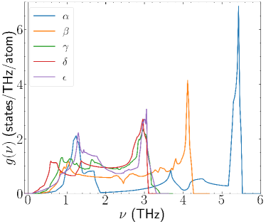
Figure 2: Phonon densities of states $g(\nu)$ for the different phases of tin at their respective equilibrium volumes using the AM05 functional.

The phonon calculations provide a rigorous way to determine model parameters in OpenSesame used to construct the full tabular EOS. We use the Debye model Debye and the ‘generalized CHART D’ Grüneisen model Thompson and Lauson (1974) within OpenSesame to construct the 2162 EOS. Typically moments of $g(\nu)$ are used to determine the Debye frequencies of the solid phases. Chisolm et al. (2003, 2005b) For tin, we found that the zeroth moment typically gave free energies $F(T)$ that matched the phonon free energy well over a wide range of temperatures and volumes, whereas the free energy predicted using first and second moments to determine the Debye frequencies did not match the phonon $F(T)$ results very well. At the same time, evaluation of the zeroth moment can be prone to numerical errors when a very small and otherwise negligible density of states is present around zero frequency (see Ref. Rehn et al., a for details). This motivated us to develop an alternative method for determining the Debye frequencies for each phase and each volume based on a minimization scheme, motivated by matching the Debye free energy to the phonon free energy as closely as possible. Given the phonon or Debye density of states $g(\nu)$, the free energy at fixed volume $V$ is

$$\small F(T;V)=\int_{0}^{\infty}g(\nu)\bigg{(}{1\over 2}h\nu+k_{B}T\ln\big{[}1-e^{-h\nu/k_{B}T}\big{]}\bigg{)}\,\mathrm{d}\nu.$$ (8)

We choose the Debye frequency $\nu_{D}$ via the minimization procedure

$$\min_{\nu_{D}}\|F_{D}(T;V)-F_{\mathrm{ph}}(T;V)\|_{2},$$ (9)

where $F_{D}$ is the Debye free energy, $F_{\mathrm{ph}}$ is the free energy from phonon calculations, $\|f(T)\|_{2}^{2}=\int_{0}^{T_{\mathrm{max}}}f^{2}(T)dT$ denotes the $L_{2}$ norm, and we use $T_{\mathrm{max}}=4000$ K. The solution is obtained via a least-squares routine. Note that we determine $\nu_{D}$ over a range of volumes, resulting in $\nu_{D}(V)$ for each solid phase. The determination of $\nu_{D}$ in this way leads to very close agreement of $F_{D}$ and $F_{\mathrm{ph}}$ over a wide range of volumes and temperatures, as shown in Fig. 3. In Fig. 3, the solid lines are computed using the Debye model, while the dots are computed from phonon calculations. We find close agreement at low and high temperatures, with slightly poorer agreement at low temperatures for small volumes. Also note that the $\nu_{D}$ determined using the minimization scheme above were in very close agreement with the zeroth moment results in cases where the zeroth moment results were not prone to numerical evaluation errors. The advantage of the minimization approach is that it is not prone to the same numerical difficulties.

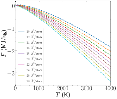
Figure 3: Free energy as a function of temperature for the $\gamma$ phase computed from phonon calculations (dots) and the corresponding Debye model fit (lines) using Eq. 9 over a range of different volumes.

The calculation of $\nu_{D}(V)$ for each phase provides a set of points that can be used to fit an analytical form that corresponds to a particular Grüneisen model in OpenSesame. In this case, we use the form

$$\nu_{D}(V)=\nu_{\mathrm{ref}}\,x^{-A}\exp\left\{-B(x-1)-{C\over 2}(x^{2}-1)\right\}$$ (10)

where $x=V/V_{\mathrm{ref}}$ and $V_{\mathrm{ref}}$ is a reference volume close to the equilibrium volume of each phase, to determine parameters for the Grüneisen model. Here the parameter $A$ is chosen to be 2/3, while $B$ and $C$ are determined by fitting Eq. 10 to the Debye frequencies. The Grüneisen parameter $\Gamma=-\mathrm{d}\ln\nu_{D}/\mathrm{d}\ln V$ is then

$$\Gamma(V)=A+Bx+Cx^{2}.$$ (11)

With this form for $\Gamma$ and fixed $A$, there are effectively two parameters that determine the Grüneisen model for each phase, $B$ and $C$, and these are determined from DFT data by fitting Eq. 10 to DFT-calculated $\nu_{D}(V)$ points. Note, however, that in OpenSesame, $B$ and $C$ are not used, but instead the Grüneisen parameter $\Gamma$ and its derivative $\Gamma^{\prime}\equiv\mathrm{d}\Gamma/\mathrm{d}\ln\rho$ are specified at a reference volume $V_{\mathrm{ref}}$ (or equivalently, reference density $\rho_{\mathrm{ref}}$). Therefore, rather than specifying the Grüneisen model through $B$ and $C$, we use $\Gamma_{\mathrm{ref}}\equiv\Gamma(\rho_{\mathrm{ref}})$ and $\Gamma_{\mathrm{ref}}^{\prime}\equiv\Gamma^{\prime}(\rho_{\mathrm{ref}})$, with values listed in Table 2. The Debye temperature $\Theta_{D}$ is also specified at the same reference density $\rho_{\mathrm{ref}}$. For the 2162 EOS, $\rho_{\mathrm{ref}}=7.581$ g/cm³ is chosen for all phases, which is within 1% of the equilibrium density $\rho_{0}$ determined from the DFT cold curve calculations. Also note that the form of $\Gamma$ in Eq. 11 is only used for $V\leq V_{\mathrm{ref}}$. Above $V_{\mathrm{ref}}$, another form for $\Gamma$ is used to prevent $\Gamma$ from diverging in the expansion region well below solid densities, such that $\Gamma\rightarrow 1$ as $V\rightarrow\infty$ (see Ref. Rehn et al., a for additional details). The values of $\Theta_{D}(\rho_{\mathrm{ref}})$, $\Gamma_{\mathrm{ref}}$, and $\Gamma^{\prime}_{\mathrm{ref}}$ for each phase are shown in Table 2. Values not in parentheses are the values computed directly from DFT calculations, while values that were changed to fit to experimental data (discussed in Sec. IV) are shown in parentheses.

The advantage of phonon calculations is that they provide a way to determine an initial set of Debye frequencies and Grüneisen model parameters in OpenSesame to generate the full tabular EOS. Additional details on the process used to fit to DFT data are provided in Ref. Rehn et al., a.

III.3 DFT-MD

All DFT-MD simulations were performed in VASP. We used an $NVT$ ensemble with a Nosé-Hoover thermostat Nosé (1984); Hoover (1985) to determine liquid isotherms and an $NVE$ ensemble to determine the melt curve using the $Z$ method. Belonoshko et al. (2006); Burakovsky et al. (2014, 2015)

For the $NVT$ simulations, we used the AM05 functional, a plane-wave energy cutoff of 250 eV, a 2 fs time step, and 4 electrons in the valence with the PAW method used to treat the core states. All simulations used 250 atoms in a cubic cell (a $5\times 5\times 5$ supercell of the conventional bcc $\delta$ phase) and the Brillouin zone was represented using the $\Gamma$ point only. A series of simulations were run at different volumes and temperatures. Fermi smearing was used for all simulations, setting the smearing width according to the fixed temperature of each simulation. Each simulation was started using the atomic positions of a liquid state that was generated from a separate DFT-MD simulation in which the solid $\delta$ phase was allowed to melt at 10,000 K over a period of time. The resulting liquid structures were then used as the initial structures at each $V,T$. A total of 8 ps were used to determine the resulting pressure, with the first 4 ps neglected to allow enough time for the system to equilibrate. The pressure was then determined through a time average of the last 4 ps using a block averaging procedure (see the Supplemental Material for details). Additional details on the DFT-MD calculations are provided in Ref. Rehn et al., a.

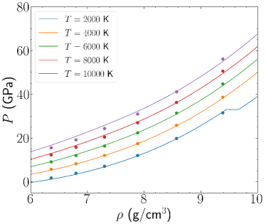
Figure 4: Isotherms from DFT-MD simulations of the liquid phase (dots) with a comparison to the 2162 EOS (lines).

Fig. 4 shows liquid isotherms computed in DFT-MD (dots), along with the isotherms used for the resulting 2162 EOS (lines). Error bars are not included with the points because the statistical errors in the pressure are small enough to fit within the dots on the plot (see the Supplemental Material for details). The isotherms help to constrain both the parameters controlling the thermal response and parameters associated with the liquid in OpenSesame. The resulting 2162 EOS fit is shown in the same figure, with overall good agreement with the DFT-MD data. Some discrepancies of the 2162 EOS and the DFT-calculated are present, which is a result of having to determine liquid model parameters that simultaneously fit the DFT-MD data and experimental Hugoniot data in the liquid phase, as described in Sec. IV. We also point out that the process for determining model parameters for the liquid phase is more involved than that of the solid phases. We leave this discussion for Sec. IV, with additional details provided in Ref. Rehn et al., a.

For the $Z$-method simulations used to determine the melt curve, we used an $NVE$ ensemble with the PBE functional and the PAW method in VASP. Since the simulations were performed at high-$PT$ conditions, we used accurate PAW potentials where the semi-core 4d states were treated as valence states, so that each Sn atom included 14 valence electrons per atom (4$d$, 5$s$, and 5$p$ orbitals). The valence states were represented with a plane-wave energy cutoff of 300 eV.

For all $Z$ method calculations involving non-cubic cells, we first relaxed the structure to determine its unit cell parameters; those unit cells were used for the construction of the corresponding supercells. We used systems of sizes 512 ($4\times 4\times 8$) for the $\beta$ phase, 504 ($6\times 6\times 7$) for the $\gamma$ phase, and 512 (rhombohedral $8\times 8\times 8$ with $\theta=109.5$ deg.) for the $\delta$ phase. Only the $\Gamma$-point was used to represent the Brillouin zone in each case. Full energy convergence (to $\sim 1$ meV/atom) was verified by performing short runs with $2\times 2\times 2$ and $3\times 3\times 3$ k-point meshes and by comparing their output with that of the run with a single $\Gamma$-point. The $Z$-method $NVE$ runs were 15,000–20,000 timesteps, with a time step of 1 fs. These points were then used to determine an analytic form for the melt curves of each solid phase, which are presented in the Supplemental Material. The full melt curve is the envelope of the three melt curves for each individual phase and is shown in Fig. 5.

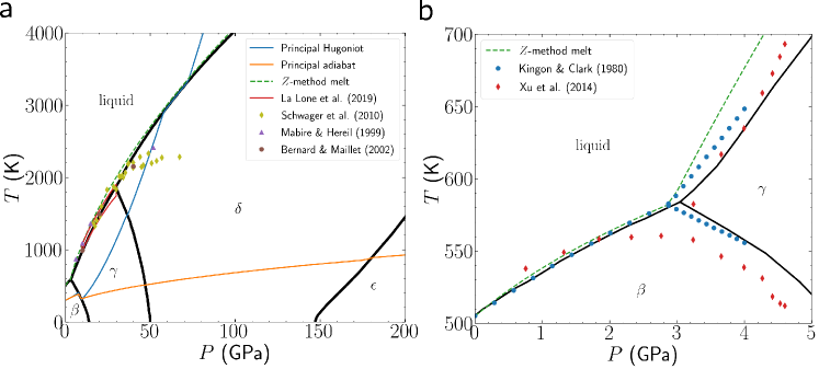
Figure 5: Phase diagram of tin. (a) A wide range of the state space with the principal Hugoniot (blue line) and principal adiabat (orange line). Experimental data of the melt curve are from Refs. La Lone et al., 2019; Schwager et al., 2010; Mabire and Hereil, 2000a, b. The data of Bernard & Maillet are MD simulations discussed in Ref. Bernard and Maillet, 2002. (b) A narrow range of the state space around the $\beta$-$\gamma$-liquid triple point. Experimental data are from Refs. Kingon et al., 1980; Xu et al., 2014.

IV Results

The DFT results presented in Sec. III provide a way to determine an initial set of parameters for models used in OpenSesame. This initial set of parameters provides a good starting point, but the DFT data will not in general agree perfectly with experimental data. The reasons for this have primarily to do with uncertainty in the exchange-correlation functional used in DFT, as well as inherent uncertainties in experiments. Different experiments can give significantly different results, making it necessary to prioritize certain experimental results based on reasonable criteria when constructing the EOS. In this section, we briefly describe the process used to adjust model parameters determined from DFT data to fit experimental results, with a focus on the resulting fit to experimental data. The final values before and after fitting are shown in Table 2, where values not in parentheses are determined directly from DFT and values in parentheses indicate that the value was adjusted to agree with experimental data. A more detailed description of this process can be found in Ref. Rehn et al., a.

IV.1 Phase diagram

We first review the overall phase diagram in $P$-$T$ space in the final 2162 EOS, shown in Fig. 5. The phase diagram generated from DFT data alone does not fit perfectly with experimental data, but the qualitative features are correct, as described in Ref. Rehn et al., a. The primary tool for adjusting the location of the phase boundaries in pressure is by adjusting the cold curve equilibrium energies $E_{0}=F_{\mathrm{cold}}(V_{0})$. The DFT-predicted values and adjusted values (in parentheses) are shown in Table 2, where the energy is relative to $E_{0}$ of the $\beta$ phase. Although the changes appear to be relatively large, there are two important reasons for this. First, it is not possible with GGA xc functionals to simultaneously predict correct atomization energies and bond lengths; Perdew et al. (2008) the prediction of both is only possible within a meta-GGA framework. The AM05 functional used for DFT calculations in Sec. III gives very accurate predictions of bond lengths for tin, but because it is a GGA, should not be expected to provide accurate relative values of $E_{0}$. Second, adjusting $E_{0}$ does not change any properties that depend on derivatives of the energy, making $E_{0}$ the most straight-forward and least problematic parameter to use to adjust the relative locations of the phase boundaries in $P$-$T$ space.

Several points regarding the phase diagram should be noted. First, the $\beta$-$\gamma$ phase boundary was modified from the SESAME 2161 EOS to be located at slightly lower pressures. The 2161 EOS originally determined the phase boundary based on shock Hugoniot data, which included some kinetic effects associated with hysteresis in the $\beta\rightarrow\gamma$ phase transition. With recent developments in modeling the kinetics of phase transitions in hydrodynamics codes, it is now important to place the phase boundary at the location of static experiments so that the kinetic effects associated with the $\beta$-$\gamma$ phase transition can be accounted for in the kinetic models, rather than in the EOS. This allows the reverse transformation ($\gamma\rightarrow\beta$) to properly include kinetic effects, as well. The $\beta$-$\gamma$ phase boundary and the $\beta$-$\gamma$-liquid triple point are shown in Fig. 5b with comparisons to experimental data from Refs. Kingon et al., 1980; Xu et al., 2014. The 2162 EOS is in close agreement with the experimental data near the triple point and with the $\beta$-$\gamma$ phase boundary. The higher pressure parts of the phase boundary are also in close agreement with phase diagrams reported previously in Refs. Tonkov and Ponyatovsky, 2018; Young, 1991; Cox and Christie, 2015.

We also point out that the slope of the $\gamma$-$\delta$ phase boundary in Fig. 5a is determined entirely from DFT data. One challenge in determining this phase boundary lies in the fact that the $\gamma$ phase cold curves should in principle be computed in such a way that the lattice is allowed to relax at each volume. This leads to a $c/a$ ratio that converges to 1 as the volume is decreased, indicating that the $\delta$ (bcc) phase becomes lower in energy. Although in principle this is the correct way to treat the $\gamma$ phase, in practice this makes it very difficult to determine a well-defined $\gamma$-$\delta$ phase boundary. At elevated temperatures the Gibbs free energy $G(P)$ of the $\gamma$ and $\delta$ phases are nearly coincident near the phase boundary, making it difficult to numerically determine the pressure $P$ associated with the transition at elevated temperatures. The ambiguity in defining a phase boundary is also borne out in experiments. In particular, Salamat et al. find in Ref. Salamat et al., 2013 evidence of the emergence of body-centered orthorhombic (bco) phase(s) near the $\gamma$-$\delta$ phase transition at room temperature. This finding indicates that near the phase boundary, the relative energy differences between bct, bco, and bcc structures are small enough that the presence of local strains within different grains of the sample can lead to the local stabilization of different phases. These results provide insight into the fundamental difficulty of defining a clear phase boundary in this region of the state space, rather than indicate a fundamental failure in the DFT calculations.

In order to address the difficulties associated with defining the $\gamma$-$\delta$ phase boundary, we ultimately used a DFT cold curve for the $\gamma$ phase in which the $c/a$ ratio is kept fixed at the equilibrium (zero pressure) value. This allows for more contrast in the enthalpies (at $T=0$) and the Gibbs free energies ($T>0$) near the phase boundary and therefore alleviates difficulties associated with the numerically ambiguous phase preference near the phase boundary.

Another point regarding the $\epsilon$ phase is also worth mentioning. The experimental evidence for the emergence of the $\epsilon$ phase is relatively limited, but DAC experiments by Salamat et al. (Ref. Salamat et al., 2011) show a clear transition to the $\epsilon$ phase at room temperature above 150 GPa. Nonetheless, these experiments do not provide information about the slope of the phase boundary in $P$-$T$ at these high pressures, making the DFT-predicted phase boundary the best currently available data we have. The DFT results clearly indicate a positive slope in Fig. 5a which is also in qualitative agreement with experiments performed by Lazicki et al. (Ref. Lazicki et al., 2015) involving dynamic compression of tin up to pressures around 1 TPa. In Ref. Lazicki et al., 2015, no evidence of the $\epsilon$ phase is found, however it is noted that very high temperatures are achieved during compression, which may mean that the $(P,T)$ states probed in experiments are located above the $\delta$-$\epsilon$ phase boundary that we compute using DFT. Furthermore, Lazicki et al. postulate that strain rates in their compressive experiments may be too fast to observe nucleation and growth of the $\epsilon$ phase. New compressive experiments would help to shed light on these issues and on the location of the phase boundary.

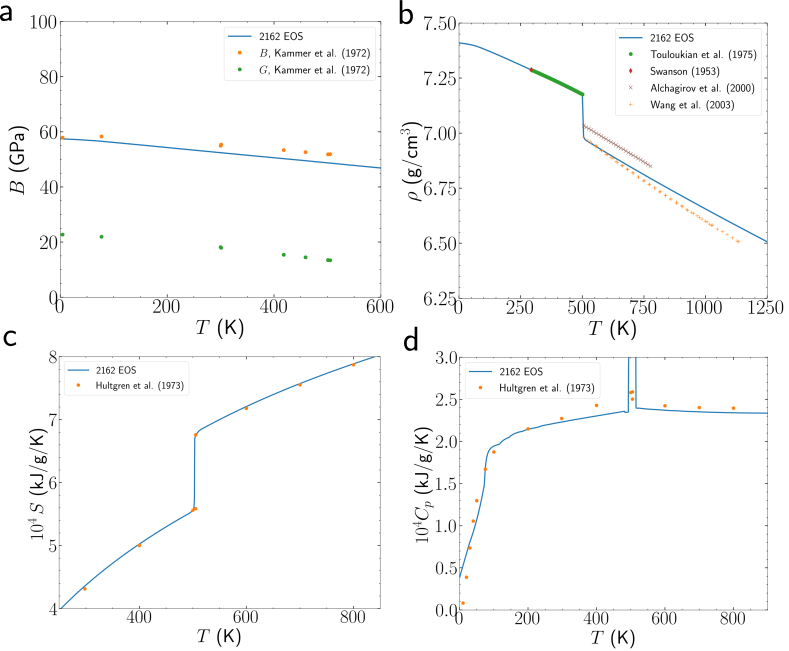
Figure 6: Comparison of the 2162 EOS to experimental isobaric data along the 1 bar isobar. (a) The bulk modulus $B(T)$ and shear modulus $G(T)$ are computed from temperature-dependent elastic constant data in Ref. Kammer et al., 1972. (b) The density $\rho(T)$ in the $\beta$ phase (below 505 K) and in the liquid phase (above 505 K) are compared to experimental data from Refs. Touloukian, 1975; Swanson, 1953; Alchagirov and Chochaeva, 2000; Wang et al., 2003. Experimental data from Ref. Hultgren et al., 1973 are compared with the 2162 EOS for (c) the entropy $S(T)$ and (d) the heat capacity at constant pressure $C_{p}(T)$.

One final point regarding the melt curve is important. Many measurements of the melt curve have been made using a variety of experimental techniques, with a large amount of scatter in the data. Due to the degree of variability, it is necessary to choose a subset of experimental results to guide the EOS construction. For the 2162 EOS we have focused on recent experiments by La Lone et al. (Ref. La Lone et al., 2019) which measure melt on shock release using a combination of pyrometry, reflectance, and velocimetry techniques to determine the location of the melt curve in $(P,T)$ space. These results are shown in Fig. 5a, where the red lines indicate upper and lower limits of uncertainty in the measurements. We also include laser-heated DAC data by Schwager et al. (Ref. Schwager et al., 2010), shock-induced melt data by Mabire & Héreil (Refs. Mabire and Hereil, 2000a, b), and classical molecular dynamics (MD) simulations of the melt by Bernard & Maillet (Ref. Bernard and Maillet, 2002). Note that the calculations of Bernard & Maillet use an interatomic potential optimized by fitting to DFT-MD simulations. We also show the melt curve predicted by our $Z$ method calculations in Fig. 5, which are in very close agreement to the 2162 EOS. Comparisons to other experiments can be found in Ref. Rehn et al., a. It is also important to point out that the melt curve of the 2162 EOS is located at slightly higher temperatures than the previous 2161 EOS, based primarily on the experimental data provided in Fig. 5 and also on a trend towards consensus that the melt curve lies at higher temperatures than what is shown in the 2161 EOS. La Lone et al. (2019); Cox and Christie (2015)

The melt curve is determined primarily by the liquid phase parameters, shown in Table 2, in addition to values of liquid-specific parameters $\Gamma_{\rm m},\Gamma_{\rm rs},T_{\rm m},T_{\rm rs}$, and $\Delta S$, described in Sec. II. For these liquid-specific parameters, we use the values $\Gamma_{\rm rs}=\Gamma_{\rm m}=2.45$, which is the same as the adjusted $\Gamma_{\mathrm{ref}}$ value for the $\gamma$ phase, as well as $T_{\rm m}=T_{\rm rs}=580$ K and $\Delta S=0.9$ kJ/g. Note that all parameters for the liquid phase in Table 2 are shown in parentheses because there is not a unique way to determine the parameters from DFT calculations. The liquid phase parameters are the least straight-forward to adjust, and we provide a brief overview of how these parameters were determined below (additional details are provided in Ref. Rehn et al., a). First, because the melt curve extends across the $\beta$, $\gamma$, and $\delta$ phases, it was necessary to construct a cold curve that interpolated between these three phases. This was done by stitching together $P(\rho)$ for the $\beta$ and $\gamma$ phases near the $T=0$ transition density (the $\delta$ phase is left out because the $\gamma$ and $\delta$ $P(\rho)$ curves are nearly overlapping at high density), so that an ‘effective’ cold curve that interpolates between phases could be used. The resulting cold curve has a slightly lower $\rho_{0}$ than the $\beta$, $\gamma$, and $\delta$ phases, as shown in Table 2. The values of $B$ and $B^{\prime}$ are also determined from fitting the Vinet-Rose model in this way. The parameters $E_{0}$ and $\Theta_{D}$ for the liquid phase mainly influence the location of the melt curve in $P$-$T$ space. Because there is no straight-forward way to determine these parameters directly from DFT data, the adjustment was done mostly through trial-and-error fitting to the experimental data of melt curve measurements. Lastly, the Grüneisen parameter $\Gamma_{\mathrm{ref}}$ was initially chosen to be the same as $\Gamma_{\mathrm{ref}}$ of the $\gamma$ phase. However, this resulted in pressures that were slightly too high at elevated temperatures in both the DFT-MD data (Fig. 3) and in the shock Hugoniot data (Fig. 8). Lowering this value by $\sim 2$% allowed for better agreement in both the DFT-MD results and the shock Hugoniot results. As described in Sec. IV.4, lowering this value changed the location of the phase boundaries in Fig. 5 slightly. We therefore reduced $\Gamma_{\mathrm{ref}}$ of the solid phases by the same ratio as was used for the liquid phase to restore the accuracy of the phase boundaries. Note that $\Gamma^{\prime}_{\mathrm{ref}}$ of the liquid phase primarily controls the curvature of the melt curve at high pressures. We determined the value $\Gamma^{\prime}_{\mathrm{ref}}=-3.5$ in Table 2 by fitting to the melt curve at high pressure. Because this value was relatively higher than that of the solid phases, $\Gamma^{\prime}_{\mathrm{ref}}$ of the solid phases were decreased to retain the shapes of the phase boundaries at high pressures.

IV.2 Isobaric data

When adjusting model parameters in OpenSesame to create the 2162 EOS, we started with isobaric data. As described in Ref. Rehn et al., a, the isobaric data generally allows for some constraints to be placed on model parameters of the phases that are stable at atmospheric pressure. For tin, this includes the $\beta$ and liquid phases.

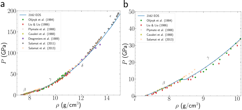
Figure 7: Room temperature isotherm for the 2162 EOS with a comparison to experimental data over (a) the full range of experimental data and (b) near the $\beta$-$\gamma$ phase transition. Experimental data are from Refs. Olijnyk and Holzapfel, 1984; Liu and Liu, 1986; Plymate et al., 1988; Cavaleri et al., 1988; Desgreniers et al., 1989; Salamat et al., 2011, 2013.

In Fig. 6, we show a variety of isobaric data at 1 bar and at temperatures above and below the $\beta$-liquid phase boundary. In Fig. 6a the temperature dependent bulk modulus $B(T)$ of the $\beta$ phase is shown with comparisons to experimental data determined from Kammer et al. (Ref. Kammer et al., 1972). Kammer et al. measured the elastic constants of $\beta$ tin at different temperatures, and from those measurements it is possible to estimate the bulk modulus $B$ and shear modulus $G$, as described in Ref. Rehn et al., a. Using the data of Kammer et al., we found that at $T=0$, $B=58$ GPa, which can be compared to the AM05 result of $B=52.7$ GPa, as found by fitting the $E$-$V$ points to a Vinet-Rose model. Vinet et al. (1987) Because the DFT result is slightly low, we modified the value to $B=58$ GPa (see Table 2), which provides a constraint that reduces the number of remaining model parameters that need to be adjusted.

In Fig. 6b, we show the density along the 1 bar isobar with comparisons to experimental data from Refs. Touloukian, 1975; Swanson, 1953; Alchagirov and Chochaeva, 2000; Wang et al., 2003. The 2162 EOS matches very well in the $\beta$ phase below melt, and lies in between the data of Alchagirov et al. and Wang et al. in the liquid phase. Due to the constraint on $B$ at $T=0$, we were able to determine the equilibrium density of the $\beta$ phase, $\rho_{0}=7.437$ g/cm³ based on the $\rho(T)$ data in Fig. 6b. This value is roughly 1.2% higher than the AM05-predicted value of 7.344 g/cm³ (see Table 2) and 7.2% higher than the PBE-predicted value of 6.939 g/cm³. The other piece that we adjusted slightly to fit to the isobaric $\rho(T)$ data is $\Gamma_{\mathrm{ref}}$, shown in Table 2. The combination of $\rho_{0}$, $B$, and $\Gamma_{\mathrm{ref}}$ together control the slope and initial value of $\rho(T)$, and these values were found to give good agreement with data shown in Fig. 6b.

We also show the entropy (Fig. 6c) and heat capacity at constant pressure (Fig. 6d) with comparisons to data from Hultgren et al. (Ref. Hultgren et al., 1973). Very close agreement is shown between the experimental data and the 2162 EOS. No additional adjustment of model parameters was necessary to provide good agreement for the $\beta$ phase.

IV.3 Isothermal data

The next step in the EOS construction is to look at isothermal DAC data at room temperature. A variety of DAC experiments have been performed over the years, and we focus specifically on data from Refs. Olijnyk and Holzapfel, 1984; Liu and Liu, 1986; Plymate et al., 1988; Cavaleri et al., 1988; Desgreniers et al., 1989; Salamat et al., 2011, 2013. In Fig. 7 we show a comparison of the 2162 EOS to these experimental results. Note that due to the high level of agreement of the AM05 cold curves with DAC data (Fig. 1), it was possible to use the AM05 cold curves directly and without any adjustments, aside from the $\beta$ phase which was modified slightly based on isobaric data. The unmodified cold curve parameters are shown in Table 2.

In Fig. 7a, we show results over a wide range of density, which spans all four solid phases included in the EOS, with the $\beta$-$\gamma$ transition occurring at roughly 9 GPa, the $\gamma$-$\delta$ transition occurring at roughly 48 GPa, and the $\delta$-$\epsilon$ transition occurring at roughly 156 GPa. The experiments of Salamat et al. (Refs. Salamat et al., 2011, 2013) are more recent and are the most precise data available, and the 2162 EOS shows a high level of agreement with these results, particularly in the $\beta$ and $\gamma$ phases at low pressure, as shown in Fig. 7b. Note that small discrepancies can be seen in the $\delta$ phase in Fig. 7a, where the 2162 EOS is slightly lower in pressure than the results of Salamat et al.. This is interesting due to the fact that the discrepancies start to appear at the onset of the $\gamma$-$\delta$ phase transition. In the experiments of Ref. Salamat et al., 2013, Salamat et al. find evidence for the emergence of bco phases, indicating that the $\gamma$ (bct), $\delta$ (bcc), and bco phases are all accessible in this region of the state space and that the observed stable phase may be influenced by small local strains present in the samples. For the purposes of the EOS, we did not try to address all of these issues, but rather relied on the AM05-calculated values, since this provided a concrete way for determining model parameters without leading to significant discrepancies with the available experimental data.

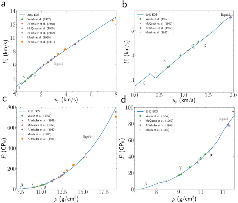
Figure 8: Comparison of the 2162 EOS to shock experiments along the principal Hugoniot. The $U_{s}$-$u_{p}$ relations are shown over (a) a wide range of shock speeds including the liquid phase and (b) over a narrow range of shock speeds focusing on the solid phases. The pressure $P(\rho)$ along the Hugoniot is shown over (c) a wide range of pressure and (d) a narrow range of pressure focusing on the solid phases. Experimental data are from Refs. Walsh et al., 1957; Al’tshuler et al., 1958; McQueen and Marsh, 1960; Al’Tshuler et al., 1962; Marsh, 1980; Al’Tshuler et al., 1981.

IV.4 Shock data

The final piece of experimental data we consider is shock data. Fig. 8 shows a comparison of the 2162 EOS to experimental shock measurements from Refs. Walsh et al., 1957; Al’tshuler et al., 1958; McQueen and Marsh, 1960; Al’Tshuler et al., 1962; Marsh, 1980; Al’Tshuler et al., 1981. Note that the principal Hugoniot is shown in Fig. 5a. In Figs. 8a-b we show the $U_{\!{}_{S}}$-$u_{\!{}_{P}}$ relations along the principal Hugoniot, where panel (a) shows a wide range of shock speeds into the liquid phase and panel (b) is zoomed in to focus on the solid phases. The 2162 EOS is in good agreement throughout. Note that in panel (b), the $\beta\rightarrow\gamma$ phase transition is shown to initiate at lower shock speed than the data points of the Marsh et al. (1980) results. As mentioned previously, this is due to the fact that some hysteresis associated with the phase transition is included in the shock data. The goal of the 2162 EOS is to place the phase boundaries at their equilibrium values and allow for hydrodynamics codes to capture the kinetic effects associated with phase transitions. We also point out that the $\gamma$-$\delta$ phase transition is very subtle, but can be seen at $U_{\!{}_{S}}\approx 4.2$ km/s in panel (b). This is not expected to be a large effect since the $\gamma$ phase exhibits a shear deformation to the $\delta$ phase along the phase boundary. One interesting remaining question is if there is any noticeable change in material strength through this phase transformation.

In Figs. 8c-d, we show the corresponding pressure dependence $P(\rho)$ along the Hugoniot. The 2162 EOS is again in good agreement with the experimental data through the three solid phases and into the liquid.

The results of Fig. 8 did not require any additional adjustments to the solid phases, but did require adjustments to the Grüneisen parameters of the liquid phase. Originally, the liquid phase was constructed using the same $\Gamma_{\mathrm{ref}}$ and $\Gamma^{\prime}_{\mathrm{ref}}$ values as the $\Gamma$ phase. However, we found that this value of $\Gamma_{\mathrm{ref}}$ caused $U_{\!{}_{S}}$ to be slightly too high at large $u_{\!{}_{P}}$ in Fig. 8a and also caused the pressure to be slightly too high at high densities in Fig. 8c. In order to address these issues, we lowered $\Gamma_{\mathrm{ref}}$ for the liquid phase from 2.48 to 2.45 (see Table 2), a change of roughly 2%, which brought the Hugoniot down in both $U_{\!{}_{P}}$ and $P$ and resulting in the agreement with experimental data shown in Fig. 8. However, because of these adjustments, the solid-solid and solid-liquid phase boundaries in Fig. 5 also changed to be in worse agreement with experimental data. To address this, we ended up decreasing the $\Gamma_{\mathrm{ref}}$ values of the $\gamma$, $\delta$, and $\epsilon$ phases by the same ratio as was used for the liquid phase (see Table 2), which restored the agreement of the phase boundaries with experimental data.

V Conclusion

We have described the construction of a new multiphase SESAME EOS for tin, referred to as SESAME 2162. The new EOS includes four solid phases and the liquid phase. We performed DFT calculations using the AM05 exchange-correlation functional of the four solid phases and the liquid phase, including cold curve and quasi-harmonic phonon calculations of the solid phases and DFT-MD calculations of the liquid phase. The DFT calculations greatly aid in constraining the model parameters used in OpenSesame to generate the resulting 2162 EOS. Because model parameters determined from DFT alone are not in exact agreement with experimental data, slight adjustments of model parameters determined by the DFT calculations are required. We presented the results of the 2162 EOS construction with comparisons to a wide range of experimental data, including isobaric data, isothermal data, shock data, measurements of the triple point and solid-solid phase boundaries, and measurements of the melt curve. The 2162 EOS shows an overall high level of agreement with these experimental results. In addition, in regions of the state space where experimental data is limited or does not exist, the DFT calculations provide the best available information on material properties. Looking forward, it will be important to develop new methods for EOS construction, such as automated EOS generation based on both DFT and experimental data. At the same time, uncertainty quantification of EOS will be important. We expect that the process used to generate the 2162 EOS can be used to inform on both uncertainty quantification and methods for automatic EOS generation, as described in more detail in Ref. Rehn et al., a.

References

- Preston et al. (2003) Dean L Preston, Davis L Tonks, and Duane C Wallace, “Model of plastic deformation for extreme loading conditions,” Journal of applied physics 93, 211–220 (2003).
- Barton et al. (2011) Nathan R Barton, Joel V Bernier, Robert Becker, Athanasios Arsenlis, Robert Cavallo, Jaime Marian, Moono Rhee, H-S Park, Bruce A Remington, and RT Olson, “A multiscale strength model for extreme loading conditions,” Journal of applied physics 109, 073501 (2011).
- Greeff (2016) CW Greeff, “A model for phase transitions under dynamic compression,” Journal of Dynamic Behavior of Materials 2, 452–459 (2016).
- Andrews (1971) DJ Andrews, “Calculation of mixed phases in continuum mechanics,” Journal of computational physics 7, 310–326 (1971).
- Wills et al. (2016) Ann Elisabet Wills, Justin Brown, and Carl LANL Greeff, Implementing and testing a Kinetic Phase Transition Model., Tech. Rep. (Sandia National Lab.(SNL-NM), Albuquerque, NM (United States), 2016).
- Lyon (1992) Stanford P Lyon, “SESAME: The Los Alamos National Laboratory equation of state database,” Los Alamos National Laboratory report LA-UR-92-3407 (1992).
- Chisolm et al. (2005a) ED Chisolm, CW Greeff, and DC George, Constructing explicit multiphase equations of state with opensesame, Tech. Rep. (Tech. Rep. LA-UR-05-9413 (Los Alamos National Laboratory), 2005).
- Greeff et al. (2005) C Greeff, E Chisolm, D George, C Greeff, E Chisolm, and D George, “SESAME 2161: An explicit multiphase equation of state for tin,” Los Alamos National Laboratory Tech. Rep. No. LA-UR-05-9414 (2005).
- Molodets and Nabatov (2000) Alexandr Mikhailovich Molodets and Sergei Sergeevich Nabatov, “Thermodynamic potentials, diagram of state, and phase transitions of tin on shock compression,” High Temperature 38, 715–721 (2000).
- Young (1991) David A Young, Phase diagrams of the elements (Univ of California Press, 1991).
- Tonkov and Ponyatovsky (2018) E Yu Tonkov and EG Ponyatovsky, Phase transformations of elements under high pressure (CRC press, 2018).
- Nikolaev et al. (1973) IN Nikolaev, VP Marin, VN Panyushkin, and LS Pavlyukov, “Characteristics of the alpha to beta sn phase transformation under pressure,” Soviet Physics-Solid State 14, 2022–2024 (1973).
- Anderson et al. (2000) William W Anderson, Frank Cverna, Robert S Hixson, John Vorthman, Mark D Wilke, George T Gray III, and Karl L Brown, “Phase transition and spall behavior in -tin,” in AIP Conference Proceedings, Vol. 505 (American Institute of Physics, 2000) pp. 443–446.
- Cornelius et al. (2017) Ben Cornelius, Shay Treivish, Yair Rosenthal, and Michael Pecht, “The phenomenon of tin pest: A review,” Microelectronics Reliability 79, 175–192 (2017).
- Kammer et al. (1972) EW Kammer, LC Cardinal, CL Vold, and ME Glicksman, “The elastic constants for single-crystal bismuth and tin from room temperature to the melting point,” Journal of Physics and Chemistry of Solids 33, 1891–1898 (1972).
- Touloukian (1975) Yeram Sarkis Touloukian, “Thermal expansion: metallic elements and alloys,” Thermophysical properties of matter 12 (1975).
- Swanson (1953) Howard Eugene Swanson, Standard X-ray diffraction powder patterns, Vol. 1 (US Department of Commerce, National Bureau of Standards, 1953).
- Alchagirov and Chochaeva (2000) Boris Batokovich Alchagirov and Asiyat Maskhutovna Chochaeva, “Temperature dependence of the density of liquid tin,” High Temperature 38, 44–48 (2000).
- Wang et al. (2003) Lianwen Wang, Qiang Wang, Aiping Xian, and Kunquan Lu, “Precise measurement of the densities of liquid bi, sn, pb and sb,” Journal of Physics: Condensed Matter 15, 777 (2003).
- Hultgren et al. (1973) Ralph Hultgren, Pramod D Desai, Donald T Hawkins, Molly Gleiser, and Kenneth K Kelley, Selected values of the thermodynamic properties of the elements, Tech. Rep. (National Standard Reference Data System, 1973).
- Thewlis and Davey (1954) J Thewlis and AR Davey, “Thermal expansion of grey tin,” Nature 174, 1011–1011 (1954).
- Prasad and Wooster (1955) SC Prasad and WA Wooster, “The study of the elastic constants of white tin by diffuse x-ray reflexion,” Acta Crystallographica 8, 682–686 (1955).
- Olijnyk and Holzapfel (1984) H Olijnyk and WB Holzapfel, “Phase transitions in si, ge and sn under pressure,” Le Journal de Physique Colloques 45, C8–153 (1984).
- Liu and Liu (1986) Ming Liu and Ling-Gun Liu, “Compressions and phase transitions of tin to half a megabar,” High Temperatures. High Pressures (Print) 18, 79–85 (1986).
- Desgreniers et al. (1989) Serge Desgreniers, Yogesh K Vohra, and Arthur L Ruoff, “Tin at high pressure: An energy-dispersive x-ray-diffraction study to 120 gpa,” Physical Review B 39, 10359 (1989).
- Plymate et al. (1988) Thomas G Plymate, James H Stout, and Mark E Cavaleri, “Pressure-volume-temperature behavior and heterogeneous equilibria of the non-quenchable body-centered tetragonal polymorph of metallic tin,” Journal of Physics and Chemistry of Solids 49, 1339–1348 (1988).
- Cavaleri et al. (1988) Mark E Cavaleri, Thomas G Plymate, and James H Stout, “A pressure-volume-temperature equation of state for sn () by energy dispersive x-ray diffraction in a heated diamond-anvil cell,” Journal of Physics and Chemistry of Solids 49, 945–956 (1988).
- Salamat et al. (2011) Ashkan Salamat, Gaston Garbarino, Agnes Dewaele, Pierre Bouvier, Sylvain Petitgirard, Chris J Pickard, Paul F McMillan, and Mohamed Mezouar, “Dense close-packed phase of tin above 157 gpa observed experimentally via angle-dispersive x-ray diffraction,” Physical Review B 84, 140104 (2011).
- Salamat et al. (2013) Ashkan Salamat, Richard Briggs, Pierre Bouvier, Sylvain Petitgirard, Agnès Dewaele, Melissa E Cutler, Furio Cora, Dominik Daisenberger, Gaston Garbarino, and Paul F McMillan, “High-pressure structural transformations of sn up to 138 gpa: Angle-dispersive synchrotron x-ray diffraction study,” Physical Review B 88, 104104 (2013).
- Stager et al. (1962) RA Stager, AS Balchan, and HG Drickamer, “High-pressure phase transition in metallic tin,” The Journal of Chemical Physics 37, 1154–1154 (1962).
- Barnett et al. (1966) J Dean Barnett, Vern E Bean, and H Tracy Hall, “X-ray diffraction studies on tin to 100 kilobars,” Journal of Applied Physics 37, 875–877 (1966).
- Vaidya and Kennedy (1970) SN Vaidya and GC Kennedy, “Compressibility of 18 metals to 45 kbar,” Journal of Physics and Chemistry of Solids 31, 2329–2345 (1970).
- Walsh et al. (1957) John M. Walsh, Melvin H. Rice, Robert G. McQueen, and Frederick L. Yarger, “Shock-wave compressions of twenty-seven metals. equations of state of metals,” Phys. Rev. 108, 196–216 (1957).
- Al’tshuler et al. (1958) LV Al’tshuler, KK Krupnikov, and MI Brazhnik, “Dynamic compressibility of metals under pressures from 400,000 to 4,000,000 atmospheres,” Sov. Phys. JETP 7, 614–619 (1958).
- McQueen and Marsh (1960) RG McQueen and SP Marsh, “Equation of state for nineteen metallic elements from shock-wave measurements to two megabars,” Journal of Applied Physics 31, 1253–1269 (1960).
- Al’Tshuler et al. (1962) LV Al’Tshuler, AA Bakanova, and RF Trunin, “Shock adiabats and zero isotherms of seven metals at high pressures,” Sov. Phys. JETP 15, 65–75 (1962).
- Marsh (1980) Stanley P Marsh, LASL shock Hugoniot data, Vol. 5 (Univ of California Press, 1980).
- Al’Tshuler et al. (1981) LV Al’Tshuler, AA Bakanova, IP Dudoladov, EA Dynin, RF Trunin, and BS Chekin, “Shock adiabatic curves of metals,” Journal of Applied Mechanics and Technical Physics 22, 145–169 (1981).
- Hu et al. (2008) Jianbo Hu, Xianming Zhou, Chengda Dai, Hua Tan, and Jiabo Li, “Shock-induced bct-bcc transition and melting of tin identified by sound velocity measurements,” Journal of Applied Physics 104, 083520 (2008).
- Rice et al. (1958) MH Rice, R Go McQueen, and JM Walsh, “Compression of solids by strong shock waves,” in Solid state physics, Vol. 6 (Elsevier, 1958) pp. 1–63.
- Lazicki et al. (2015) Amy Lazicki, JR Rygg, Federica Coppari, Ray Smith, Dayne Fratanduono, RG Kraus, GW Collins, R Briggs, DG Braun, DC Swift, et al., “X-ray diffraction of solid tin to 1.2 tpa,” Physical review letters 115, 075502 (2015).
- Kingon et al. (1980) AI Kingon, KINGON AI, and CLARK JB, “A redetermination of the melting curve of tin to 3.7 gpa,” (1980).
- Xu et al. (2014) Liang Xu, Yan Bi, Xuhai Li, Yuan Wang, Xiuxia Cao, Lingcang Cai, Zhigang Wang, and Chuanmin Meng, “Phase diagram of tin determined by sound velocity measurements on multi-anvil apparatus up to 5 gpa and 800 k,” Journal of Applied Physics 115, 164903 (2014).
- Barnett et al. (1963) J Dean Barnett, Roy B Bennion, and H Tracy Hall, “X-ray diffraction studies on tin at high pressure and high temperature,” Science 141, 1041–1042 (1963).
- Hinton et al. (2020) Jasmine K Hinton, Christian Childs, Dean Smith, Paul B Ellison, Keith V Lawler, and Ashkan Salamat, “Response of the mode grüneisen parameters with anisotropic compression: A pressure and temperature dependent raman study of -sn,” Physical Review B 102, 184112 (2020).
- Price et al. (1971) DL Price, JM Rowe, and RM Nicklow, “Lattice dynamics of grey tin and indium antimonide,” Physical Review B 3, 1268 (1971).
- Rowe (1967) JM Rowe, “Crystal dynamics of metallic -sn at 110 k,” Physical Review 163, 547 (1967).
- Ivanov et al. (1987) AS Ivanov, A Yu Rumiantsev, B Dorner, NL Mitrofanov, and VV Pushkarev, “Lattice dynamics and electron-phonon interaction in -tin,” Journal of Physics F: Metal Physics 17, 1925 (1987).
- Ivanov et al. (1995) AS Ivanov, NL Mitrofanov, and A Yu Rumiantsev, “Fermi surface and fine structure of the phonon dispersion curves of white tin,” Physica B: Condensed Matter 213, 423–426 (1995).
- Giefers et al. (2007) Hubertus Giefers, Elizabeth A Tanis, Sven P Rudin, Carl Greeff, Xuezhi Ke, Changfeng Chen, Malcolm F Nicol, Michael Pravica, Walter Pravica, Jiyong Zhao, et al., “Phonon density of states of metallic sn at high pressure,” Physical review letters 98, 245502 (2007).
- Mabire and Hereil (2000a) Catherine Mabire and Pierre L Hereil, “Shock induced polymorphic transition and melting of tin,” in AIP Conference Proceedings, Vol. 505 (American Institute of Physics, 2000) pp. 93–96.
- Mabire and Hereil (2000b) C Mabire and P-L Hereil, “Shock induced polymorphic transition and melting of tin up to 53 gpa (experimental study and modelling),” Le Journal de Physique IV 10, Pr9–749 (2000b).
- Seagle et al. (2013) CT Seagle, J-P Davis, MR Martin, and HL Hanshaw, “Shock-ramp compression: Ramp compression of shock-melted tin,” Applied Physics Letters 102, 244104 (2013).
- Briggs et al. (2019) R Briggs, MG Gorman, S Zhang, D McGonegle, AL Coleman, F Coppari, MA Morales-Silva, RF Smith, JK Wicks, CA Bolme, et al., “Coordination changes in liquid tin under shock compression determined using in situ femtosecond x-ray diffraction,” Applied Physics Letters 115, 264101 (2019).
- Héreil and Mabire (2002) Pierre-Louis Héreil and Catherine Mabire, “Temperature measurement of tin under shock compression,” in AIP Conference Proceedings, Vol. 620 (American Institute of Physics, 2002) pp. 1235–1238.
- Dudley and Hall (1960) J Duane Dudley and H Tracy Hall, “Experimental fusion curves of indium and tin to 105 000 atmospheres,” Physical Review 118, 1211 (1960).
- Weir et al. (2012) ST Weir, MJ Lipp, S Falabella, G Samudrala, and YK Vohra, “High pressure melting curve of tin measured using an internal resistive heating technique to 45 gpa,” Journal of Applied Physics 111, 123529 (2012).
- La Lone et al. (2019) BM La Lone, PD Asimow, OV Fat’yanov, RS Hixson, GD Stevens, WD Turley, and LR Veeser, “High-pressure melt curve of shock-compressed tin measured using pyrometry and reflectance techniques,” Journal of Applied Physics 126, 225103 (2019).
- Jayaraman et al. (1963) A Jayaraman, W Klement Jr, and GC Kennedy, “Melting and polymorphism at high pressures in some group iv elements and iii-v compounds with the diamond/zincblende structure,” Physical Review 130, 540 (1963).
- Narushima et al. (2007) T Narushima, T Hattori, T Kinoshita, A Hinzmann, and K Tsuji, “Pressure dependence of the structure of liquid sn up to 19.4 gpa,” Physical Review B 76, 104204 (2007).
- Briggs et al. (2012) R Briggs, D Daisenberger, A Salamat, G Garbarino, M Mezouar, M Wilson, and PF McMillan, “Melting of sn to 1 mbar,” in Journal of Physics: Conference Series, Vol. 377 (IOP Publishing, 2012) p. 012035.
- Briggs et al. (2017) R Briggs, D Daisenberger, OT Lord, Ashkan Salamat, E Bailey, MJ Walter, and PF McMillan, “High-pressure melting behavior of tin up to 105 gpa,” Physical Review B 95, 054102 (2017).
- Schwager et al. (2010) Beate Schwager, Marvin Ross, Stefanie Japel, and Reinhard Boehler, “Melting of sn at high pressure: Comparisons with pb,” The Journal of chemical physics 133, 084501 (2010).
- De Rességuier et al. (2007) T De Rességuier, Loïc Signor, A Dragon, M Boustie, G Roy, and F Llorca, “Experimental investigation of liquid spall in laser shock-loaded tin,” Journal of applied physics 101, 013506 (2007).
- Signor et al. (2010) Loïc Signor, Thibaut de Rességuier, André Dragon, Gilles Roy, Alain Fanget, and Matthieu Faessel, “Investigation of fragments size resulting from dynamic fragmentation in melted state of laser shock-loaded tin,” International Journal of Impact Engineering 37, 887–900 (2010).
- Corkill et al. (1991) Jennifer L Corkill, Alberto Garca, and Marvin L Cohen, “Theoretical study of high-pressure phases of tin,” Physical Review B 43, 9251 (1991).
- Hafner (1974) J Hafner, “Ab initio calculation of the pressure-induced a4 a5 a2 (distorted) a3 phase transitions in tin,” Physical Review B 10, 4151 (1974).
- Ihm and Cohen (1981) J Ihm and Marvin L Cohen, “Equilibrium properties and the phase transition of grey and white tin,” Physical Review B 23, 1576 (1981).
- Cheong and Chang (1991) BH Cheong and Kee-Joo Chang, “First-principles study of the structural properties of sn under pressure,” Physical Review B 44, 4103 (1991).
- Christensen (1993) NE Christensen, “The body-centered tetragonal high-pressure phase of tin,” Solid state communications 85, 151–154 (1993).
- Christensen and Methfessel (1993) NE Christensen and M Methfessel, “Density-functional calculations of the structural properties of tin under pressure,” Physical Review B 48, 5797 (1993).
- Aguado (2003) Andrés Aguado, “First-principles study of elastic properties and pressure-induced phase transitions of sn: Lda versus gga results,” Physical Review B 67, 212104 (2003).
- Yu et al. (2006) Chun Yu, Junyan Liu, Hao Lu, and Junmei Chen, “Ab initio calculation of the properties and pressure induced transition of sn,” Solid state communications 140, 538–543 (2006).
- Cui et al. (2008) Shouxin Cui, Lingcang Cai, Wenxia Feng, Haiquan Hu, Changzheng Wang, and Yuanxu Wang, “First-principles study of phase transition of tin and lead under high pressure,” physica status solidi (b) 245, 53–57 (2008).
- Yao and Klug (2011) Yansun Yao and Dennis D Klug, “Prediction of a bcc–hcp phase transition for sn: A first-principles study,” Solid state communications 151, 1873–1876 (2011).
- Wehinger et al. (2014) Björn Wehinger, Alexeï Bosak, Giuseppe Piccolboni, Keith Refson, Dmitry Chernyshov, Alexandre Ivanov, Alexander Rumiantsev, and Michael Krisch, “Diffuse scattering in metallic tin polymorphs,” Journal of Physics: Condensed Matter 26, 115401 (2014).
- Rowe et al. (1965) JM Rowe, BN Brockhouse, and EC Svensson, “Lattice dynamics of white tin,” Physical Review Letters 14, 554 (1965).
- Chen (1967) SH Chen, “Group-theoretical analysis of lattice vibrations in metallic -sn,” Physical Review 163, 532 (1967).
- Pavone et al. (1998) Pasquale Pavone, Stefano Baroni, and Stefano de Gironcoli, “ phase transition in tin: A theoretical study based on density-functional perturbation theory,” Physical Review B 57, 10421 (1998).
- Bernard and Maillet (2002) S Bernard and JB Maillet, “First-principles calculation of the melting curve and hugoniot of tin,” Physical Review B 66, 012103 (2002).
- Zhang et al. (2011) Lin Zhang, Ying-Hua Li, Yu-Ying Yu, Xue-Mei Li, Yun Ma, Cheng-Gang Gu, Cheng-Da Dai, and Ling-Cang Cai, “General construction of mean-field potential and its application to the multiphase equations of state of tin,” Physica B: Condensed Matter 406, 4163–4169 (2011).
- Ravelo and Baskes (1997) R Ravelo and M Baskes, “Equilibrium and thermodynamic properties of grey, white, and liquid tin,” Physical Review Letters 79, 2482 (1997).
- Soulard and Durand (2020) Laurent Soulard and O Durand, “Observation of phase transitions in shocked tin by molecular dynamics,” Journal of Applied Physics 127, 165901 (2020).
- Buy et al. (2006) Francois Buy, Christophe Voltz, and Fabrice Llorca, “Thermodynamically based equation of state for shock wave studies: application to the design of experiments on tin,” in AIP Conference Proceedings, Vol. 845 (American Institute of Physics, 2006) pp. 41–44.
- Cox (2006) GA Cox, “A multi-phase equation of state and strength model for tin,” in AIP Conference Proceedings, Vol. 845 (American Institute of Physics, 2006) pp. 208–211.
- Khishchenko (2008) KV Khishchenko, “Equation of state and phase diagram of tin at high pressures,” in Journal of Physics: Conference Series, Vol. 121 (IOP Publishing, 2008) p. 022025.
- Cox and Christie (2015) GA Cox and Michael Andrew Christie, “Fitting of a multiphase equation of state with swarm intelligence,” Journal of Physics: Condensed Matter 27, 405201 (2015).
- Rehn et al. (a) Daniel A Rehn, Carl W Greeff, Daniel G Sheppard, and Scott D Crockett, Using density functional theory to construct multiphase equations of state: tin as an example, Tech. Rep., LA-UR-20-29170 (2020). doi:10.2172/1711355.
- Vinet et al. (1987) Pascal Vinet, John R Smith, John Ferrante, and James H Rose, “Temperature effects on the universal equation of state of solids,” Physical Review B 35, 1945 (1987).
- (90) P. Debye, “Zur theorie der spezifischen wärmen,” Annalen der Physik 344, 789–839.
- Chisolm (2003) ED Chisolm, Thomas–Fermi–Dirac theory as calculated in the EOS-production programs Grizzly and Opensesame, Tech. Rep. (Report no. LA-UR-05-2297, Los Alamos: Los Alamos National Lab, 2003).
- Thomas (1927) Llewellyn H Thomas, “The calculation of atomic fields,” in Mathematical Proceedings of the Cambridge Philosophical Society, Vol. 23 (Cambridge University Press, 1927) pp. 542–548.
- Fermi (1927) Enrico Fermi, “Un metodo statistico per la determinazione di alcune priorieta dell’atome,” Rend. Accad. Naz. Lincei 6, 32 (1927).
- Dirac (1930) Paul AM Dirac, “Note on exchange phenomena in the thomas atom,” in Mathematical Proceedings of the Cambridge Philosophical Society, Vol. 26 (Cambridge University Press, 1930) pp. 376–385.
- Chisolm et al. (2005b) E Chisolm, S Crockett, and D Wallace, Extending the CCW EOS I: Extending the Cold and Nuclear Contributions to High Compression, Tech. Rep. (LA-UR-03-7344, Los Alamos National Laboratory, 2005).
- Grover (1971) Richard Grover, “Liquid metal equation of state based on scaling,” The Journal of Chemical Physics 55, 3435–3441 (1971).
- Kresse and Hafner (1993) Georg Kresse and Jürgen Hafner, “Ab initio molecular dynamics for liquid metals,” Physical Review B 47, 558 (1993).
- Kresse and Hafner (1994) Georg Kresse and Jürgen Hafner, “Ab initio molecular-dynamics simulation of the liquid-metal–amorphous-semiconductor transition in germanium,” Physical Review B 49, 14251 (1994).
- Kresse and Furthmüller (1996a) Georg Kresse and Jürgen Furthmüller, “Efficiency of ab-initio total energy calculations for metals and semiconductors using a plane-wave basis set,” Computational materials science 6, 15–50 (1996a).
- Kresse and Furthmüller (1996b) Georg Kresse and Jürgen Furthmüller, “Efficient iterative schemes for ab initio total-energy calculations using a plane-wave basis set,” Physical review B 54, 11169 (1996b).
- Blöchl (1994) Peter E Blöchl, “Projector augmented-wave method,” Physical review B 50, 17953 (1994).
- Kresse and Joubert (1999) Georg Kresse and Daniel Joubert, “From ultrasoft pseudopotentials to the projector augmented-wave method,” Physical review b 59, 1758 (1999).
- Methfessel and Paxton (1989) M. Methfessel and A. T. Paxton, “High-precision sampling for brillouin-zone integration in metals,” Phys. Rev. B 40, 3616–3621 (1989).
- Wills et al. (2010) John M Wills, Mebarek Alouani, Per Andersson, Anna Delin, Olle Eriksson, and Oleksiy Grechnyev, Full-Potential Electronic Structure Method: energy and force calculations with density functional and dynamical mean field theory, Vol. 167 (Springer Science & Business Media, 2010).
- Rehn et al. (2020) Daniel A Rehn, John M Wills, Torey E Battelle, and Ann E Mattsson, “Dirac’s equation and its implications for density functional theory based calculations of materials containing heavy elements,” Physical Review B 101, 085114 (2020).
- Rehn et al. (b) Daniel A Rehn, Torbjörn Björkman, Ann E Wills, and John M Wills, Relativistic density functional theory in the full potential linear muffin tin orbital method, Tech. Rep., LA-UR-19-32606 (2020). doi:10.2172/1595363.
- Armiento and Mattsson (2005) Rickard Armiento and Ann E Mattsson, “Functional designed to include surface effects in self-consistent density functional theory,” Physical Review B 72, 085108 (2005).
- Perdew et al. (1996) John P Perdew, Kieron Burke, and Matthias Ernzerhof, “Generalized gradient approximation made simple,” Physical Review Letters 77, 3865 (1996).
- Belonoshko et al. (2006) Anatoly B Belonoshko, NV Skorodumova, Anders Rosengren, and Börje Johansson, “Melting and critical superheating,” Physical Review B 73, 012201 (2006).
- Burakovsky et al. (2014) L Burakovsky, SP Chen, DL Preston, and DG Sheppard, “Z methodology for phase diagram studies: platinum and tantalum as examples,” in J. Phys. Conf. Ser, Vol. 500 (2014) p. 162001.
- Burakovsky et al. (2015) L Burakovsky, N Burakovsky, and DL Preston, “Ab initio melting curve of osmium,” Physical Review B 92, 174105 (2015).
- (112) Leonid Burakovsky, To be published.
- Dove (1993) Martin T Dove, Introduction to lattice dynamics, Vol. 4 (Cambridge University Press, 1993).
- Togo and Tanaka (2015) A Togo and I Tanaka, “First principles phonon calculations in materials science,” Scr. Mater. 108, 1–5 (2015).
- Monkhorst and Pack (1976) Hendrik J Monkhorst and James D Pack, “Special points for brillouin-zone integrations,” Physical review B 13, 5188 (1976).
- Thompson and Lauson (1974) SL Thompson and HS Lauson, Improvements in the CHART D radiation-hydrodynamic code III: Revised analytic equations of state, Tech. Rep. (Sandia Labs., 1974).
- Chisolm et al. (2003) Eric D Chisolm, Scott D Crockett, and Duane C Wallace, “Test of a theoretical equation of state for elemental solids and liquids,” Physical Review B 68, 104103 (2003).
- Nosé (1984) Shuichi Nosé, “A unified formulation of the constant temperature molecular dynamics methods,” The Journal of chemical physics 81, 511–519 (1984).
- Hoover (1985) William G Hoover, “Canonical dynamics: Equilibrium phase-space distributions,” Physical review A 31, 1695 (1985).
- Perdew et al. (2008) John P Perdew, Adrienn Ruzsinszky, Gábor I Csonka, Oleg A Vydrov, Gustavo E Scuseria, Lucian A Constantin, Xiaolan Zhou, and Kieron Burke, “Restoring the density-gradient expansion for exchange in solids and surfaces,” Physical review letters 100, 136406 (2008).