Initial Data and Eccentricity Reduction Toolkit for
Binary Black Hole Numerical Relativity Waveforms

Abstract

The production of numerical relativity waveforms that describe quasi-circular binary black hole mergers requires high-quality initial data, and an algorithm to iteratively reduce residual eccentricity. To date, these tools remain closed source, or in commercial software that prevents their use in high performance computing platforms. To address these limitations, and to ensure that the broader numerical relativity community has access to these tools, herein we provide all the required elements to produce high-quality numerical relativity simulations in supercomputer platforms, namely: open source parameter files to numerical simulate spinning black hole binaries with asymmetric mass-ratios; open source Python tools to produce high-quality initial data for numerical relativity simulations of spinning black hole binaries on quasi-circular orbits; open source Python tools for eccentricity reduction, both as stand-alone software and deployed in the Einstein Toolkit’s software infrastructure. This open source toolkit fills in a critical void in the literature at a time when numerical relativity has an ever increasing role in the study and interpretation of gravitational wave sources. As part of our community building efforts, and to streamline and accelerate the use of these resources, we provide tutorials that describe, step by step, how to obtain and use these open source numerical relativity tools.

1 Introduction

Numerical relativity [1, 2, 3, 4] plays a central role in contemporary gravitational wave astrophysics [5, 6, 7, 8]. The use of numerical relativity waveforms has been essential to develop approximate waveform models that are extensively used for gravitational wave detection and parameter estimation [9, 10, 11, 12, 13]. The construction of numerical relativity waveforms catalogs [14, 15, 16, 17, 18, 19] has enabled in-depth analyses of the astrophysical properties of gravitational wave sources [20, 21, 22, 23].

As gravitational wave astrophysics continues to probe the gravitational wave spectrum [24, 25, 26, 27, 28], numerical relativity will be essential to enable and interpret new discoveries, enlighten our understanding of the physics of these sources, and provide constraints that may further establish general relativity or favor alternatives theories of gravity [29, 30, 31].

Advancing our understanding of gravitational wave sources depends critically on the production of high quality numerical relativity waveforms that, in the case of binary black hole mergers, span an 8-D parameter space that includes mass-ratio, two 3-D vectors that define the individual spin of the binary components, and orbital eccentricity, $(q,\,\mathbf{s}_{1},\,\mathbf{s}_{2},\,e)$, respectively. It is then apparent that despite the existence of thousands of numerical relativity waveforms, we need to be creative about how to combine them to densely sample these high dimensional signal manifold [32, 33]. It is also clear that we need to continue producing numerical relativity waveforms to describe sources whose parameters are not accurately captured by existing approximate waveform models or available numerical relativity waveforms.

In order to empower the broader numerical relativity community to participate in the construction of numerical relativity waveform catalogs, we introduce open source Python libraries that have been tested and deployed within the Einstein Toolkit [34] to streamline and accelerate these activities. This approach builds upon our previous software development that consisted of open source Python libraries to post-process numerical relativity data to extract the waveform strain at future null infinity [35]. These combined tools provide the required end-to-end software infrastructure to utilize the Einstein Toolkit for the construction of high-quality numerical relativity waveform catalogs.

This manuscript is organized as follows. Section 2 describes our approach to construct high-quality initial data, and to post-process the data products of numerical relativity simulations to remove residual eccentricity. We put these tools at work in Section 3, where we show that we can produce nearly circular initial data, and that our method for eccentricity reduction produces waveforms with eccentricities of order ${\cal{O}}\sim 10^{-4}$ after just one iteration. We summarize this work, and outline future research directions in Section 4. We present a tutorial that describes how to obtain and use these libraries in A.

2 Methods

In this section we describe the approach followed to produce high-quality initial data for binary black hole simulations. Thereafter, we briefly introduce the method used for eccentricity reduction.

2.1 Initial Data Production

The first guess for the tangential, $p_{t}$, and radial, $p_{r}$, components of momenta for the black hole binary system are generated using techniques presented in [36] and [37]. They extract momenta components from Hamilton’s equations of motion in post-Newtonian (PN) theory, combined with high-PN-order expressions for the gravitational-wave flux, $dE_{\rm GW}/dt$, and the tidal energy injected into the black holes, $dM/dt$.

The Hamiltonian contains orbital [38], spin-orbit [38, 39, 40], spin-spin [38, 41, 42], and spin-spin-spin [43] terms up to and including 3.5PN order.

The high-PN-order expressions for $dE_{\rm GW}/dt$ incorporate nonspinning and precessing-spin terms [44, 45], and are adjusted to account for the tidal energy injected into the black holes $dM/dt$  [46].

The above expressions were implemented in the open-source, Python-based NRPyPN software, which is part of NRPy+ (“Python-based code generation for numerical relativity… and beyond!”) [47]. A tutorial for using the software is given in A.1 below. In short, the expression for tangential momentum $p_{t}(r)$ up to and including 3.5PN order is taken from  [36] and validated up to 3PN order against [37], and up to 3.5PN order against the original Mathematica notebooks used by  [36].

Meanwhile, the expression for radial momentum $p_{r}$ up to and including 3.5PN order is derived in NRPyPN as follows. First, Hamilton’s equations of motion imply that

$$\frac{dr}{dt}=\frac{\partial H}{\partial p_{r}}.$$ (1)

Next we Taylor expand $\partial H/\partial p_{r}$ in powers of $p_{r}$, about $p_{r}=0$, to obtain (to first order in $p_{r}$):

$$p_{r}\approx\left(\frac{dr}{dt}-\left.\frac{\partial H}{\partial p_{r}}\right|_{p_{r}=0}\right)\left(\left.\frac{\partial^{2}H}{\partial p_{r}^{2}}\right|_{p_{r}=0}\right)^{-1}\,,$$ (2)

where

$$\frac{dr}{dt}=\left(\frac{dE_{\rm GW}}{dt}+\frac{dM}{dt}\right)\left[\frac{dH_{\rm circ}}{dr}\right]^{-1}\,,$$ (3)

and

$$\frac{dH_{\rm circ}(r,p_{t}(r))}{dr}=\frac{\partial H(p_{r}=0)}{\partial r}+\frac{\partial H(p_{r}=0)}{\partial p_{t}}\frac{\partial p_{t}}{\partial r}\,,$$ (4)

are given explicitly in terms of binary input parameters and $M\Omega$ (as given to 3.5PN order by [36]).

2.2 Eccentricity Reduction

The algorithm we describe in this section was introduced in [36], and was originally developed as a Mathematica notebook. As part of this work, we have re-written this eccentricity reduction method using Python libraries, optimized it, and tailored it to conduct automated, large-scale, numerical relativity campaigns on high performance computing platforms.

This eccentricity reduction method is applied to remove eccentricity from a numerical relativity simulation whose initial data were produced with the method described in the previous section. Once the numerical simulation has progressed enough, typically between $500\textrm{M}$ to $600\textrm{M}$ of evolution, we process the relevant data files, as described in A, to compute correction factors, $\lambda_{t},\lambda_{r}$, of the initial components of the momenta $p^{0}_{t}$ and $p^{0}_{r}$.

To compute $\lambda_{t},\lambda_{r}$ we assume that oscillations induced as a result of eccentricity in the orbital frequency, $\Omega$, take the form

$$\mathcal{R}_{\Omega}=A+B\cos(\Omega_{r}t+\Psi)\,,$$ (5)

where $A$, $B$ and $\Psi$ are coefficients to be determined, and $\Omega_{r}$ is the frequency of the radial oscillations. Using the 1PN order quasi-Keplerian parametrization [48], we can obtain closed form expressions for these correction factors

$$\lambda_{t}=1+\left[\frac{B}{4\Omega_{0}}-\gamma\frac{B(3\eta+1)}{8r_{0}\Omega_{0}}\right]\cos\Psi,$$ (6)

$$\lambda_{r}=1+\frac{B\eta}{2r_{0}^{1/2}\Omega_{0}\left|p^{0}_{r}\right|}\left[1+\gamma\frac{1}{r_{0}}\right]\sin\Psi,$$ (7)

where $\eta=m_{1}m_{2}/(m_{1}+m_{2})$ is the symmetric mass ratio, $(m_{1},\,m_{2})$ represent the masses of the binary components, $r_{0}$ is the initial orbital separation, and $\Omega_{0}$ is the quasi-circular initial orbital frequency calculated at 3.5PN order [36]. In A.1 we describe how to use simulation data and analytical approximations to compute the correction factors $\lambda_{t}$ and $\lambda_{r}$.

3 Results

In this section we combine the tools described above for initial data production and eccentricity reduction. We selected three binary black hole systems whose properties are described in Table 1. Notice that these systems span three different mass-ratios, $q\in\{1,\,3\}$, and several spinning, non-precessing configurations.

The results presented in Table 1 show that for all the binary systems under consideration, our toolkit produces systems whose initial eccentricities are $e_{0}\sim 10^{-3}$. Furthermore, these eccentricity values are reduced to $e_{0}\sim 10^{-4}$ after just one iteration. In other words, these ready-to-use tools produce high-quality numerical relativity waveforms after a minimal number of iterations.

$\textrm{D}\,[\textrm{M}]$	($\chi_{1}^{x},\chi_{1}^{y},\chi_{1}^{z}$)	($\chi_{2}^{x},\chi_{2}^{y},\chi_{2}^{z}$)	$q$	Iter #	$p_{r}\,[\times 10^{-4}]$	$p_{\phi}\,[\times 10^{-2}]$	$e_{0}\,[\times 10^{-3}]$
11.0	(0.0, 0.0, -0.4)	(0.0, 0.0, -0.5)	1.0	0	-8.60	9.293	2.43
S_q_1				1	-7.70	9.284	0.74
9.0	(0.0, 0.0, 0.4)	(0.0, 0.0, -0.5)	3.0	0	-7.50	7.652	1.70
S_q_3				1	-6.60	7.650	0.71

Table 1: Summary of the astrophysical and orbital parameters of three binary black hole systems used to test our open source toolkit for the production of initial data and eccentricity reduction. Notice that in all cases the initial eccentricity is of order $e_{0}\sim{\cal{O}}\left(10^{-3}\right)$ for the zeroth iteration, and it is reduced to $e_{0}\sim{\cal{O}}\left(10^{-4}\right)$ after just one iteration.

Figure 1 present two types of results. The left panels present results for the eccentricity estimator $e_{\Omega}$ of the orbital frequency ad defined in Eq. (3.13) of [36]. These results show, as discussed previously, that even the zeroth iteration is already nearly circular. The right panels present waveforms of the first iteration extracted at future null infinity [35].

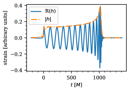
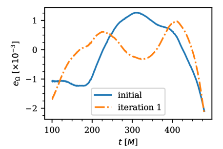
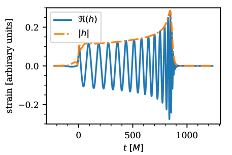
Figure 1: Top panels: results of the eccentricity reduction procedure for simulation S_q_1. Top-left panel: eccentricity estimator results for the zeroth and first iterations. Top-right panel: gravitational wave signal, extracted at future null infinity, after eccentricity reduction. Bottom panels: as top panels, but for simulation S_q_3.

These results indicate that the open source tools presented in this article, along with the tutorials and configuration files released with this work, will provide the required building blocks to engage a broader cross section of the numerical relativity community in the production of large scale numerical relativity waveform catalogs.

4 Conclusions

Numerical relativity simulations [1, 2, 3] of binary black hole mergers were produced a decade before the first gravitational wave detection of these astrophysical events was realized by the advanced LIGO detectors [24]. Over the last decade, numerical relativity software stacks have matured to the point of automating and streamlining the production of large-scale numerical relativity catalogs [14, 15, 16, 17, 18, 19]. Nonetheless, the available number of numerical relativity waveforms is not sufficient to densely cover the high dimensional signal manifold spanned by these astrophysical events.

Furthermore, essential tools to produce initial data and to automate eccentricity reduction continue to be kept as closed source software or licensed software. Neither of these solutions is adequate if we aim to enable a larger cross section of the numerical relativity community to participate in the production of numerical relativity waveforms to accurately infer the astrophysical properties of compact binary sources. This need will become a pressing issue as advanced gravitational wave detectors gradually reach design sensitivity, and the number of detections reaches the expected number of one event for every fifteen minutes of searched data.

The deployment of these tools as stand-alone software and within the Einstein Toolkit is aligned with our community building efforts, and marks another milestone in our program for the production of an end-to-end software framework that enables users to produce high quality initial data, automate eccentricity reduction, and post-process numerical relativity data products to extract numerical relativity waveforms at future null infinity [35]. These user-friendly tools will allow new users to engage in the development of open source numerical relativity software, using the Einstein Toolkit as the driver for such community building activities.

5 Acknowledgements

EAH gratefully acknowledges National Science Foundation (NSF) awards OAC-1931561 and OAC-1934757. RH gratefully acknowledges NSF awards OAC-1550514, OAC-2004879, and ACI-1238993. This research is part of the Blue Waters sustained-petascale computing project, which is supported by the NSF awards OCI-0725070 and ACI-1238993, and the State of Illinois. Blue Waters is a joint effort of the University of Illinois at Urbana-Champaign and its National Center for Supercomputing Applications. We acknowledge support from the NCSA and the Students Pushing INnovation (SPIN) undergraduate internship Program at NCSA. We thank the NCSA Gravity Group for useful feedback. NSF-1659702 and XSEDE TG-PHY160053 grants are gratefully acknowledged.

Appendix A Step by Step Tutorial

A.1 Initial Data Production

NRPyPN is part of the open-source NRPy+ (“Python-based code generation for numerical relativity… and beyond!”) [47], and provides the zeroth estimate for low-eccentricity initial data in this paper. To obtain this estimate from NRPyPN, first clone the NRPy+ github repository:

git clone https://github.com/zachetienne/nrpytutorial.git

Then (assuming that Python 2 or 3 is installed with pip), install SymPy [49] and Jupyter:

pip install -U sympy jupyter

Next, from within the nrpytutorial/NRPyPN/ directory, run

jupyter notebook NRPyPN.ipynb

A Jupyter notebook will open, in which the binary black hole initial data parameters for initial separation, spins, and mass ratio can be specified in the code cell at the bottom of the notebook. When the code cell is run (Shift+Enter), the radial $p_{r}$ and tangential momenta $p_{t}$ to 3.5 post-Newtonian order (largely following [36] but fully documented in the linked Jupyter notebooks) will be output. These momenta can be directly inserted into a Bowen-York binary black hole initial data solver (the TwoPunctures thorn was used in this work). For example, for a binary orbiting in the $xy$-plane with black holes initially located on the $x$-axis at $x=\pm a$ (with the center of mass at the origin, $x=y=z=0$), $\pm|p_{r}|$ will correspond to the $x$-component of momentum $p_{x}$ for the puncture at $x=\mp a$, respectively. Also one may choose $\pm|p_{t}|$ to correspond to the $y$-component of momentum $p_{y}$ for the puncture at $x=\pm a$ or $\mp a$, depending on whether a clockwise or a counterclockwise orbit is desired.

A.2 Eccentricity Reduction

Our eccentricity code is a available as a Python3 module on GitHub [50]

git clone https://github.com/ncsagravity/eccred

Then, assuming Python 3 is installed, run:

python
>>> import EccRed
>>> EccRed.ComputeCorrections("output_glob", MinTime=X, MaxTime=Y)

where output_glob is a shell pattern (glob) that matches all directories containing output files, MinTime and MaxTime are time bounds. For best results, MinTime should be shortly after any “junk” radiation has pass from the vicinity of the black holes and any initial gauge transition has settled, MaxTime should be close to the time plunge occurs.

Four correction values as well as the estimated eccentricity will be returned from EccRed.ComputeCorrections. In order, they are $\lambda_{r}$, $\lambda_{t}$ computed using two different methods (from PN expansion and from an eccentricity estimator respectively), and $\delta R$, the correction factors to radial and tangential momentum components and (additive) correction to initial orbital separation respectively. These corrections can then be applied to the respective initial values.

The code expects to two sets of files in the output directories: (i) a file TwoPunctures.bbh as produced by the TwoPunctures thorn that describes the parameters of the initial black holes, and (ii) a set of puncture location files puncturetracker-pt_loc..asc as produced by the PunctureTracker thorn. Columns pt_loc_x[0], pt_loc_x[1] etc., are expected to contain the location of the original plus and minus punctures. This matches the setup in [51].

In the event that EccRed.ComputeCorrections throws a runtime error, a likely solution is to adjust MinTime or MaxTime to better characterize the time domain of inspiral.

A.3 Automated Eccentricity Reduction

To simplify automation the process of eccentricity reduction using Simulation Factory [52] the Python module can be called as a command line script

./EccRed.py --tmin X --tmax X --input-parfile "input_parameter_file" \
            --output-parfile "output_parameter_file" "output_glob"

which automatically applies the correction factors to TwoPunctures’ radial and tangential momentum parameters found in input_parameter_file and produces a new parameter file in output_parameter_file.

We provide a fragment of code in RunScript.part that can be inserted into Simulation Factory’s run script files to automate the process of extending a simulation until sufficiently much data has been produced, estimating eccentricity, computing correction factors, applying them to the parameter file and submitting a new round of eccentricity reduction.

The fragment contains placeholders @ECC_TARGET@ and @ECC_TIME@ for the estimated eccentricity at which to stop the iteration and the time for which to simulate before applying the correction algorithm:

sim create --define ECC_TARGET "ECC_TARGET" --define ECC_TIME "ECC_TIME" ...

which starts the automated process.

References

- [1] F. Pretorius, “Evolution of binary black hole spacetimes,” Phys. Rev. Lett., vol. 95, p. 121101, 2005.
- [2] M. Campanelli, C. Lousto, P. Marronetti, and Y. Zlochower, “Accurate evolutions of orbiting black-hole binaries without excision,” Phys. Rev. Lett., vol. 96, p. 111101, 2006.
- [3] J. G. Baker, J. Centrella, D.-I. Choi, M. Koppitz, and J. van Meter, “Gravitational wave extraction from an inspiraling configuration of merging black holes,” Phys. Rev. Lett., vol. 96, p. 111102, 2006.
- [4] V. Cardoso, L. Gualtieri, C. Herdeiro, and U. Sperhake, “Exploring New Physics Frontiers Through Numerical Relativity,” Living Rev. Relativity, vol. 18, p. 1, 2015.
- [5] U. Sperhake, “The numerical relativity breakthrough for binary black holes,” Class. Quant. Grav., vol. 32, no. 12, p. 124011, 2015.
- [6] J. Centrella, J. G. Baker, B. J. Kelly, and J. R. van Meter, “Black-hole binaries, gravitational waves, and numerical relativity,” Rev. Mod. Phys., vol. 82, p. 3069, 2010.
- [7] T. W. Baumgarte and S. L. Shapiro, Numerical Relativity: Solving Einstein’s Equations on the Computer. Cambridge University Press, 2010.
- [8] M. Alcubierre, Introduction to 3+1 Numerical Relativity. Oxford University Press, 2008.
- [9] M. Hannam, P. Schmidt, A. Bohé, L. Haegel, S. Husa, F. Ohme, G. Pratten, and M. Pürrer, “Simple Model of Complete Precessing Black-Hole-Binary Gravitational Waveforms,” Phys. Rev. Lett., vol. 113, no. 15, p. 151101, 2014.
- [10] A. Bohé et al., “Improved effective-one-body model of spinning, nonprecessing binary black holes for the era of gravitational-wave astrophysics with advanced detectors,” Phys. Rev., vol. D95, no. 4, p. 044028, 2017.
- [11] S. Khan, S. Husa, M. Hannam, F. Ohme, M. Pürrer, X. Jiménez Forteza, and A. Bohé, “Frequency-domain gravitational waves from nonprecessing black-hole binaries. II. A phenomenological model for the advanced detector era,” Phys. Rev., vol. D93, no. 4, p. 044007, 2016.
- [12] J. Blackman, S. E. Field, M. A. Scheel, C. R. Galley, C. D. Ott, M. Boyle, L. E. Kidder, H. P. Pfeiffer, and B. Szilágyi, “Numerical relativity waveform surrogate model for generically precessing binary black hole mergers,” Phys. Rev., vol. D96, no. 2, p. 024058, 2017.
- [13] S. Husa, S. Khan, M. Hannam, M. Pürrer, F. Ohme, X. Jiménez Forteza, and A. Bohé, “Frequency-domain gravitational waves from nonprecessing black-hole binaries. I. New numerical waveforms and anatomy of the signal,” Phys. Rev., vol. D93, no. 4, p. 044006, 2016.
- [14] A. H. Mroue et al., “Catalog of 174 Binary Black Hole Simulations for Gravitational Wave Astronomy,” Phys. Rev. Lett., vol. 111, no. 24, p. 241104, 2013.
- [15] J. Healy, C. O. Lousto, Y. Zlochower, and M. Campanelli, “The RIT binary black hole simulations catalog,” Class. Quant. Grav., vol. 34, no. 22, p. 224001, 2017.
- [16] M. Boyle et al., “The SXS Collaboration catalog of binary black hole simulations,” Class. Quant. Grav., vol. 36, no. 19, p. 195006, 2019.
- [17] J. Healy, C. O. Lousto, J. Lange, R. O’Shaughnessy, Y. Zlochower, and M. Campanelli, “Second RIT binary black hole simulations catalog and its application to gravitational waves parameter estimation,” Phys. Rev. D, vol. 100, no. 2, p. 024021, 2019.
- [18] E. Huerta et al., “Physics of eccentric binary black hole mergers: A numerical relativity perspective,” Phys. Rev. D, vol. 100, no. 6, p. 064003, 2019.
- [19] K. Jani, J. Healy, J. A. Clark, L. London, P. Laguna, and D. Shoemaker, “Georgia Tech Catalog of Gravitational Waveforms,” Class. Quant. Grav., vol. 33, no. 20, p. 204001, 2016.
- [20] P. Kumar, J. Blackman, S. E. Field, M. Scheel, C. R. Galley, M. Boyle, L. E. Kidder, H. P. Pfeiffer, B. Szilagyi, and S. A. Teukolsky, “Constraining the parameters of GW150914 and GW170104 with numerical relativity surrogates,” Phys. Rev. D, vol. 99, no. 12, p. 124005, 2019.
- [21] B. Abbott et al., “Directly comparing GW150914 with numerical solutions of Einstein’s equations for binary black hole coalescence,” Phys. Rev. D, vol. 94, no. 6, p. 064035, 2016.
- [22] J. Lange et al., “Parameter estimation method that directly compares gravitational wave observations to numerical relativity,” Phys. Rev. D, vol. 96, no. 10, p. 104041, 2017.
- [23] G. Lovelace et al., “Modeling the source of GW150914 with targeted numerical-relativity simulations,” Class. Quant. Grav., vol. 33, no. 24, p. 244002, 2016.
- [24] B. Abbott et al., “GWTC-1: A Gravitational-Wave Transient Catalog of Compact Binary Mergers Observed by LIGO and Virgo during the First and Second Observing Runs,” Phys. Rev. X, vol. 9, no. 3, p. 031040, 2019.
- [25] B. Abbott et al., “GW170817: Observation of Gravitational Waves from a Binary Neutron Star Inspiral,” Phys. Rev. Lett., vol. 119, no. 16, p. 161101, 2017.
- [26] B. Abbott et al., “GW190425: Observation of a Compact Binary Coalescence with Total Mass ,” Astrophys. J. Lett., vol. 892, no. 1, p. L3, 2020.
- [27] R. Abbott et al., “GW190412: Observation of a Binary-Black-Hole Coalescence with Asymmetric Masses,” 4 2020.
- [28] R. Abbott et al., “GWTC-2: Compact Binary Coalescences Observed by LIGO and Virgo During the First Half of the Third Observing Run,” 10 2020.
- [29] M. Okounkova, L. C. Stein, J. Moxon, M. A. Scheel, and S. A. Teukolsky, “Numerical relativity simulation of GW150914 beyond general relativity,” Phys. Rev. D, vol. 101, no. 10, p. 104016, 2020.
- [30] N. Yunes, K. Yagi, and F. Pretorius, “Theoretical Physics Implications of the Binary Black-Hole Mergers GW150914 and GW151226,” Phys. Rev. D, vol. 94, no. 8, p. 084002, 2016.
- [31] R. Nair, S. Perkins, H. O. Silva, and N. Yunes, “Fundamental Physics Implications for Higher-Curvature Theories from Binary Black Hole Signals in the LIGO-Virgo Catalog GWTC-1,” Phys. Rev. Lett., vol. 123, no. 19, p. 191101, 2019.
- [32] V. Varma, S. E. Field, M. A. Scheel, J. Blackman, L. E. Kidder, and H. P. Pfeiffer, “Surrogate model of hybridized numerical relativity binary black hole waveforms,” Phys. Rev. D, vol. 99, no. 6, p. 064045, 2019.
- [33] N. E. Rifat, S. E. Field, G. Khanna, and V. Varma, “Surrogate model for gravitational wave signals from comparable and large-mass-ratio black hole binaries,” Phys. Rev. D, vol. 101, no. 8, p. 081502, 2020.
- [34] F. Löffler, J. Faber, E. Bentivegna, T. Bode, P. Diener, R. Haas, I. Hinder, B. C. Mundim, C. D. Ott, E. Schnetter, G. Allen, M. Campanelli, and P. Laguna, “The Einstein Toolkit: a community computational infrastructure for relativistic astrophysics,” Classical and Quantum Gravity, vol. 29, p. 115001, June 2012.
- [35] D. Johnson, E. Huerta, and R. Haas, “Python Open Source Waveform Extractor (POWER): An open source, Python package to monitor and post-process numerical relativity simulations,” Class. Quant. Grav., vol. 35, no. 2, p. 027002, 2018.
- [36] A. Ramos-Buades, S. Husa, and G. Pratten, “Simple procedures to reduce eccentricity of binary black hole simulations,” Phys. Rev. D, vol. 99, no. 2, p. 023003, 2019.
- [37] J. Healy, C. O. Lousto, H. Nakano, and Y. Zlochower, “Post-Newtonian Quasicircular Initial Orbits for Numerical Relativity,” Class. Quant. Grav., vol. 34, no. 14, p. 145011, 2017.
- [38] A. Buonanno, Y. Chen, and T. Damour, “Transition from inspiral to plunge in precessing binaries of spinning black holes,” Phys. Rev. D, vol. 74, p. 104005, 2006.
- [39] T. Damour, P. Jaranowski, and G. Schaefer, “Hamiltonian of two spinning compact bodies with next-to-leading order gravitational spin-orbit coupling,” Phys. Rev. D, vol. 77, p. 064032, 2008.
- [40] J. Hartung and J. Steinhoff, “Next-to-next-to-leading order post-Newtonian spin-orbit Hamiltonian for self-gravitating binaries,” Annalen Phys., vol. 523, pp. 783–790, 2011.
- [41] J. Steinhoff, S. Hergt, and G. Schaefer, “On the next-to-leading order gravitational spin(1)-spin(2) dynamics,” Phys. Rev. D, vol. 77, p. 081501, 2008.
- [42] J. Steinhoff, S. Hergt, and G. Schaefer, “Spin-squared Hamiltonian of next-to-leading order gravitational interaction,” Phys. Rev. D, vol. 78, p. 101503, 2008.
- [43] M. Levi and J. Steinhoff, “Leading order finite size effects with spins for inspiralling compact binaries,” JHEP, vol. 06, p. 059, 2015.
- [44] L. Blanchet, “Gravitational Radiation from Post-Newtonian Sources and Inspiralling Compact Binaries,” Living Rev. Rel., vol. 17, p. 2, 2014.
- [45] S. Ossokine, M. Boyle, L. E. Kidder, H. P. Pfeiffer, M. A. Scheel, and B. Szilágyi, “Comparing post-Newtonian and numerical relativity precession dynamics,” Phys. Rev. D , vol. 92, p. 104028, Nov. 2015.
- [46] D. Brown, S. Fairhurst, B. Krishnan, R. Mercer, R. Kopparapu, L. Santamaria, and J. Whelan, “Data formats for numerical relativity waves,” 9 2007.
- [47] I. Ruchlin, Z. B. Etienne, and T. W. Baumgarte, “SENR/NRPy+: Numerical relativity in singular curvilinear coordinate systems,” Phys. Rev. D , vol. 97, p. 064036, Mar. 2018.
- [48] T. Damour and N. Deruelle, “General relativistic celestial mechanics of binary systems. I. The post-Newtonian motion.,” Ann. Inst. Henri Poincaré Phys. Théor., Vol. 43, No. 1, p. 107 - 132, 1985.
- [49] A. Meurer, C. P. Smith, M. Paprocki, O. Čertík, S. B. Kirpichev, M. Rocklin, A. Kumar, S. Ivanov, J. K. Moore, S. Singh, T. Rathnayake, S. Vig, B. E. Granger, R. P. Muller, F. Bonazzi, H. Gupta, S. Vats, F. Johansson, F. Pedregosa, M. J. Curry, A. R. Terrel, v. Roučka, A. Saboo, I. Fernando, S. Kulal, R. Cimrman, and A. Scopatz, “Sympy: symbolic computing in python,” PeerJ Computer Science, vol. 3, p. e103, Jan. 2017.
- [50] S. Habib, E. Huerta, R. Haas, and E. Zachariah, “Automated framework to produce low eccentricity numerical binary black hole simulations,” Nov. 2020.
- [51] B. Wardell, I. Hinder, and E. Bentivegna, “Simulation of GW150914 binary black hole merger using the Einstein Toolkit,” Sept. 2016.
- [52] “SimFactory: Herding numerical simulations.”