Quasars That Have Transitioned from Radio-quiet to Radio-loud on Decadal Timescales Revealed by VLASS and FIRST

Abstract

We have performed a search over 3440 deg² of Epoch 1 (2017–2019) of the Very Large Array Sky Survey to identify unobscured quasars in the optical ($0.2<z<3.2$) and obscured active galactic nuclei (AGN) in the infrared that have brightened dramatically in the radio over the past one to two decades. These sources would have been previously classified as “radio-quiet” quasars based on upper limits from the Faint Images of the Radio Sky at Twenty Centimeters survey (1993–2011), but they are now consistent with “radio-loud” quasars ($L_{\rm 3\,GHz}=10^{40-42}\,\,{\rm erg}\,{\rm s}^{-1}$). A quasi-simultaneous, multiband ($\sim 1-18$ GHz) follow-up study of 14 sources with the VLA has revealed compact sources ($<0.1^{\prime\prime}$ or $<$1 kpc) with peaked radio spectral shapes. The high-amplitude variability over decadal timescales at 1.5 GHz (100% to $>$2500%), but roughly steady fluxes over a few months at 3 GHz, are inconsistent with extrinsic variability due to propagation effects, thus favoring an intrinsic origin. We conclude that our sources are powerful quasars hosting compact/young jets. This challenges the generally accepted idea that “radio-loudness” is a property of the quasar/AGN population that remains fixed on human timescales. Our study suggests that frequent episodes of short-lived AGN jets that do not necessarily grow to large scales may be common at high redshift. We speculate that intermittent but powerful jets on subgalactic scales could interact with the interstellar medium, possibly driving feedback capable of influencing galaxy evolution.

1 Introduction

Until recently, synoptic surveys of the dynamic sky have been dominated by optical, X-ray, and gamma-ray observing campaigns, with systematic radio studies of transient and variable sources, in particular those at high redshift, often performed as follow-up in response to a shorter wavelength trigger. Thus, the slow transient (or slowly varying) extragalactic radio source population remains largely unexplored, particularly among sources invisible to synoptic surveys conducted at shorter wavelengths (e.g., due to obscuration by dense columns of gas and dust). Large-scale synoptic radio surveys are thus a key way forward for both current radio telescopes, such as the Karl G. Jansky Very Large Array (VLA), and prospective instruments under development over the next decade, such as the next-generation Very Large Array (ngVLA; Murphy et al. 2018; Selina et al. 2018) and Square Kilometre Array (SKA; Dewdney et al. 2009; Braun et al. 2015, 2019).

Active Galactic Nuclei (AGN) represent the most dominant source of variability and transient activity in the radio sky (e.g. Carilli et al. 2003; Thyagarajan et al. 2011; Bannister et al. 2011; Frail et al. 2012; Bell et al. 2015; Mooley et al. 2016). The majority of AGN exhibit variability (a well-known multiwavelength hallmark of an AGN Hovatta et al. 2007) in the radio regime at the few tens of percent level over a wide range of timescales, between a few days and a few decades (e.g. Barvainis et al. 2005; Thyagarajan et al. 2011; Gralla et al. 2020; Sarbadhicary et al. 2020). This variability is often attributed to extrinsic effects related to propagation (e.g. interstellar scattering) or intrinsic effects directly related to AGN itself (Bignall et al. 2015, and references therein) such as the propagation of shocks along the jet (e.g. Marscher & Gear 1985).

More extreme radio AGN variability (with a variability amplitude $\gtrsim 100$%) occurring over longer timescales of years to decades has also been observed (e.g. Barvainis et al. 2005), and may be caused by jets that have reoriented themselves toward our line of sight or young, expanding jets that have been recently triggered. In the case of jet reorientation, precession due to perturbations from the presence of a binary SMBH or stochastic effects related to accretion (An et al., 2013) may alter the jet inclination angle and degree of Doppler boosting, thereby leading to high-amplitude, long-term variability. Bonafide candidates for new jet activity have also been identified (Mooley et al., 2016; Kunert-Bajraszewska et al., 2020), suggesting that short-lived, intermittent AGN jet activity recurring on timescales of $\sim 10^{4}-10^{5}$ years could be common, consistent with predictions (e.g. Reynolds & Begelman 1997; Czerny et al. 2009).

Compact radio AGN with subgalactic extents residing in gas-rich host galaxies, especially those at redshifts of 1$\lesssim z\lesssim 3$, are an important, yet still poorly studied class of objects for understanding the role of jet-ISM feedback in influencing galaxy growth and evolution (Mukherjee et al. 2016; Nyland et al. 2018; Jarvis et al. 2019). Specifically, the prevalence of radio AGN variability driven by different intrinsic effects, as well as the magnitude and impact feedback from subgalactic jets on SMBH-galaxy co-evolution, remain uncertain.

Here, we present follow-up, quasi-simultaneous, multiband VLA observations of a subset of AGN with high-amplitude (100% to $>$2500%) radio variability identified in a search for transients on decades-long timescales between the Faint Images of the Sky at Twenty centimeters (FIRST; Becker et al. 1995) and $\sim$3,440 deg² of Epoch 1 of the Very Large Array Sky Survey (VLASS; Lacy et al. 2020). We describe our sample and selection criteria in Section 2. In Section 3, we describe the observing and data reduction heuristics for our new multiband VLA observations. An assessment of the radio continuum properties of our sources, variability, and multiband spectral energy distributions (SEDs) is provided in Section 4. We consider a variety of possibilities for the origin of the radio variability in our sources in Section 5, and discuss implications for the life cycles of radio AGN and their connection to galaxy evolution in Section 6. We summarize our results and assess prospects for further insights through future follow-up observations in Section 7. We adopt a standard $\Lambda$CDM cosmology with $H_{0}$ = 67.7 km s^-1 Mpc^-1, $\Omega_{\Lambda}$ = 0.691 and $\Omega_{\textrm{\small{M}}}$ = 0.307 (Planck Collaboration et al., 2016) throughout our study. Errors shown are 1$\sigma$ unless otherwise stated.

2 Sample

As part of our ongoing compilation of radio transients observed at 3 GHz in Epoch 1 of VLASS, which will be presented in its entirety in Dong et al. (in prep.), we have selected a preliminary sample of radio AGN exhibiting extreme variability on timescales of $\sim$1–2 decades. In the remainder of this section, we provide details on the radio surveys used to conduct our search for variable AGN and describe our sample selection criteria.

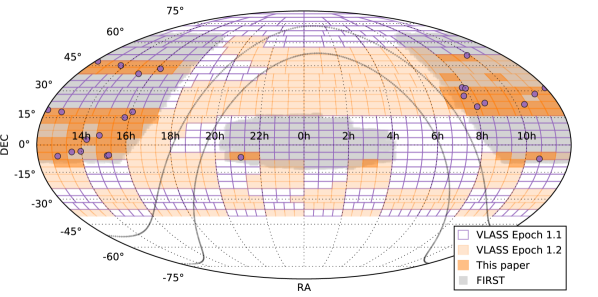
Figure 1: Relative sky footprints of the VLASS and FIRST surveys. VLASS tiles from Epochs 1.1 and 1.2 are shown in purple and light orange, respectively. The large gray shaded regions illustrate the coverage of the FIRST survey. The 86 tiles from VLASS Epoch 1.2 analyzed in this paper are indicated by the dark orange regions. The gray curves denote coordinates within 10 degrees of the Galactic plane. The positions of our 26 candidate radio-variable AGN identified via comparison with data from FIRST are shown by the purple circles.

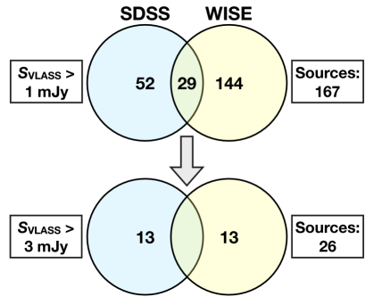
Figure 2: Venn diagram illustrating the selection criteria for our sample of AGN that have recently brightened in the radio in the last 1–2 decades. Previously radio-quiet AGN are selected based on both optical and infrared AGN diagnostics in SDSS and WISE, respectively. Further details are provided in Section 2.2.

2.1 Radio Surveys

2.1.1 FIRST

FIRST is a 20 cm (1.4 GHz) survey conducted with the pre-upgrade VLA covering a total sky footprint of 10,575 deg² (Becker et al., 1995; Helfand et al., 2015). FIRST observed approximately 9,000 deg² of the north Galactic cap from 1993–2004, and a smaller $\sim 2.5\arcdeg$-wide strip of the south Galactic cap along the Celestial equator in 2009–2011. The VLA was undergoing the upgrade of its receivers during the latter time range, leading to slightly different image characteristics in the different regions of sky covered by FIRST, but the quality of the survey’s sky coverage in the northern and southern regions are functionally equivalent. FIRST images have a resolution of approximately 5″, rms sensitivity of approximately 0.15 mJy beam^-1, and astrometric uncertainty of $\lesssim 1\arcsec$. The published catalog of emission components from FIRST is 95% complete to 2 mJy and 80% complete to the catalog limit of 1 mJy. Peak flux densities and integrated flux densities in the published catalog were determined from two-dimensional Gaussian fits to each co-added FIRST image.

2.1.2 VLASS

VLASS is a wide-area (33,885 deg²), high-resolution (2.5^′′), full-polarization, broadband radio continuum survey currently being carried out by NRAO at $S$-band (2–4 GHz). The relative sky footprints of FIRST and VLASS are illustrated in Figure 1. In order to enable transient science, a key science goal of the survey, VLASS observations are being taken over a series of 3 epochs with a cadence of 32 months. Each VLASS epoch reaches a $1\sigma$ sensitivity of 0.12 mJy beam^-1, comparable to the depth of FIRST.

VLASS Epoch 1 observations have recently been completed (2017–2019), and preliminary “QuickLook” images have been made publicly available on the NRAO archive. The VLASS QuickLook images have flux uncertainties up to $\sim 20$% and are not final survey data products (see Lacy et al. 2020 for details). Despite the limitations of the QuickLook images, they are valuable for identifying transient and variable sources that have experienced substantial changes in flux (larger than a factor of 2) in the time period between FIRST and VLASS.

2.2 Variable AGN Selection Criteria

Currently, no “official” source catalog for VLASS has been made publicly available. We therefore produced our own source catalog over a subset of VLASS Epoch 1.2 covering an area of $\sim$3,440 deg². We used the source finding algorithm PyBDSF to compile a raw VLASS catalog based on the QuickLook images of sources brighter than 1 mJy. Although our goal is to identify sources that have recently brightened in the radio, we note that similar studies of reverse transients (i.e. sources that were previously detected in FIRST but discovered to have declined drastically in flux when re-observed in VLASS 1-2 decades later) are also currently in progress (e.g. Law et al. 2018; Cendes 2020).

We performed a positional cross-match (within a radius of $1^{\prime\prime}$) with the FIRST catalog. The high prevalence of artifacts (uncleaned sidelobes) in the VLASS QuickLook images poses a challenge for reliable source extraction. We manually vetted our preliminary catalog of VLASS-FIRST transients by eye to remove spurious VLASS sources associated with image artifacts or diffuse emission (radio lobes) with inherently ill-defined positions. Such spurious sources account for the vast majority ($\sim$80–90%) of our preliminary transient catalog. Our manually-vetted catalog covering the 3,440 deg² of VLASS Epoch 1 analyzed thus far contains $\sim$2000 candidate transients that are compact and brighter than 1 mJy in VLASS but below the formal detection threshold ($1$ mJy) of FIRST. Additional details will be presented in Dong et al. (in prep.).

Table 1: Sample

Source	RA	Dec	$z$	$L_{\rm Bol}$	$\log(M_{\rm SMBH})$	$L_{\rm Bol}/L_{\rm Edd}$	Type
	(J2000)	(J2000)		(erg s-1)	(M⊙)
(1)	(2)	(3)	(4)	(5)	(6)	(7)	(8)
J0742+2704	115.701796	27.070113	0.6264	45.57	8.67	-1.20	SDSS, WISE
J0751+3154	117.877557	31.904037	1.8640	46.57	9.47	-1.00	SDSS, WISE
J0800+3124	120.044683	31.415871	1.9368	46.93	9.56	-0.73	SDSS, WISE
J0807+2102	121.767970	21.035786	1.5588	46.31	9.34	-1.13	SDSS, WISE
J0832+2302	128.198513	23.042816	0.9430	$\cdots$	$\cdots$	$\cdots$	SDSS, WISE
J0950+5128	147.653173	51.477212	0.2142	45.18	7.98	-0.90	SDSS
J1023+2219	155.842720	22.321296	$\cdots$	$\cdots$	$\cdots$	$\cdots$	WISE
J1037-0736	159.491631	-7.607362	$\cdots$	$\cdots$	$\cdots$	$\cdots$	WISE
J1112+2809	168.055854	28.165137	$\cdots$	$\cdots$	$\cdots$	$\cdots$	WISE
J1157+3142	179.388528	31.707514	0.8910	$\cdots$	$\cdots$	$\cdots$	SDSS, WISE
J1204+1918	181.218737	19.306199	2.3440	$\cdots$	$\cdots$	$\cdots$	SDSS, WISE
J1208+4741	182.241352	47.698944	1.0915	$\cdots$	$\cdots$	$\cdots$	SDSS, WISE
J1246+1805	191.518270	18.089036	$\cdots$	$\cdots$	$\cdots$	$\cdots$	WISE
J1254-0606	193.521438	-6.109209	$\cdots$	$\cdots$	$\cdots$	$\cdots$	WISE
J1333-0349	203.334269	-3.832307	$\cdots$	$\cdots$	$\cdots$	$\cdots$	WISE
J1347+4505	206.836689	45.098706	$\cdots$	$\cdots$	$\cdots$	$\cdots$	WISE
J1357-0329	209.443830	-3.484817	$\cdots$	$\cdots$	$\cdots$	$\cdots$	WISE
J1413+0257	213.454848	2.953648	$\cdots$	$\cdots$	$\cdots$	$\cdots$	WISE
J1447+0512	221.817580	5.207433	1.7475	46.36	9.02	-0.76	SDSS, WISE
J1507-0549	226.962335	-5.819718	$\cdots$	$\cdots$	$\cdots$	$\cdots$	WISE
J1512-0533	228.096364	-5.550100	$\cdots$	$\cdots$	$\cdots$	$\cdots$	WISE
J1514+4000	228.520730	40.013724	2.1226	46.80	9.74	-1.04	SDSS
J1546+1500	236.641541	15.010193	$\cdots$	$\cdots$	$\cdots$	$\cdots$	WISE
J1603+1809	240.828155	18.151432	3.2460	$\cdots$	$\cdots$	$\cdots$	SDSS
J1609+4306	242.441175	43.106462	$\cdots$	$\cdots$	$\cdots$	$\cdots$	WISE
J2109-0644	317.320264	-6.743461	1.0812	46.38	9.05	-0.77	SDSS

Note. — Column 1: Source name. Columns 2 and 3: Source right ascension and declination. Column 4: Spectroscopic redshift from SDSS DR14 from Pâris et al. (2018). Column 5: Bolometric quasar luminosity. Column 6: Virial supermassive black hole mass estimate from SDSS spectroscopy from Shen et al. (2011). Column 7: Eddington ratio. Column 8: AGN type. Sources are classified as AGN on the basis of optical spectroscopy from SDSS ((Pâris et al., 2018) and/or infrared colors based on data from WISE (Assef et al., 2018).

Table 2: FIRST and VLASS Properties

Source	DateFIRST	$\sigma_{\rm FIRST}$	$F_{\rm FIRST}$	DateVLASS	$\sigma_{\rm VLASS}$	$F_{\rm VLASS}$	$\log(L_{\rm VLASS})$
		(mJy beam-1)	(mJy beam-1)		(mJy beam-1)	(mJy beam-1)	(erg s-1)
(1)	(2)	(3)	(4)	(5)	(6)	(7)	(8)
J0742+2704	1995 Nov 10	0.166	0.53	2019 Apr 10	0.146	9.19	41.68
J0751+3154	1995 Oct 23	0.148	$<$ 0.44	2019 Apr 13	0.148	3.00	42.36
J0800+3124	1994 Jun 04	0.123	0.38	2019 Apr 13	0.125	4.54	42.58
J0807+2102	1998 Sep	0.157	$<$ 0.47	2019 Apr 14	0.137	3.69	42.26
J0832+2302	1995 Dec 28	0.157	0.48	2019 Apr 13	0.130	3.08	41.64
J0950+5128	1997 Apr 29	0.148	$<$ 0.44	2019 Apr 18	0.126	8.77	40.57
J1023+2219	1996 Jan	0.205	0.65	2019 Apr 18	0.145	3.50	$\cdots$
J1037-0736	2002 Jun	0.136	$<$ 0.41	2019 Apr 16	0.151	12.95	$\cdots$
J1112+2809	1995 Nov 04	0.156	0.49	2019 Apr 13	0.120	3.19	$\cdots$
J1157+3142	1994 Jun 06	0.601	2.02	2019 Apr 14	0.135	8.58	42.03
J1204+1918	1999 Nov	0.149	0.48	2019 Mar 21	0.145	5.09	42.84
J1208+4741	1997 Apr 05	0.157	$<$ 0.47	2019 Apr 15	0.117	3.20	41.82
J1246+1805	1999 Nov 24	0.147	$<$ 0.44	2019 Apr 12	0.122	7.09	$\cdots$
J1254-0606	2001 Apr	0.144	0.46	2019 Mar 07	0.247	8.76	$\cdots$
J1333-0349	1998 Sep	0.14	$<$ 0.42	2019 Mar 24	0.175	3.09	$\cdots$
J1347+4505	1997 Mar 03	0.151	$<$ 0.45	2019 Mar 19	0.129	3.58	$\cdots$
J1357-0329	1998 Sep	0.156	0.49	2019 Mar 24	0.170	3.11	$\cdots$
J1413+0257	1998 Jul	0.142	0.47	2019 Apr 02	0.229	6.91	$\cdots$
J1447+0512	2000 Feb	0.16	0.49	2019 Mar 12	0.152	4.30	42.45
J1507-0549	2001 Apr	0.139	$<$ 0.42	2019 Mar 07	0.159	4.73	$\cdots$
J1512-0533	2001 Apr	0.233	$<$ 0.70	2019 Mar 07	0.200	3.25	$\cdots$
J1514+4000	1994 Aug 21	0.141	$<$ 0.42	2019 Mar 28	0.164	3.49	42.57
J1546+1500	1999 Dec	0.144	$<$ 0.43	2019 Apr 11	0.122	4.69	$\cdots$
J1603+1809	1999 Nov	0.148	$<$ 0.44	2019 Apr 12	0.116	3.61	43.03
J1609+4306	1994 Jul 24	0.124	0.45	2019 May 04	0.126	4.53	$\cdots$
J2109-0644	1997 Feb 28	0.153	$<$ 0.46	2019 Apr 05	0.170	18.30	42.57

Note. — Column 1: Source name. Column 2: Date of FIRST observation. For some sources, only the year and month are provided in the header of the FIRST image. Column 3: Local 1$\sigma$ rms noise in FIRST. Column 4: Peak flux density at 1.4 GHz from FIRST. Newly identified sources in VLASS that have faint FIRST counterparts with peak flux densities $>3\sigma_{\rm FIRST}$ are reported as detections. All other sources are reported as FIRST upper limits. We note that none of the sources in this table meet the selection criteria of the FIRST catalog (Helfand et al., 2015). Column 5: Date of VLASS observation. Column 6: Local 1$\sigma$ rms noise in VLASS. Column 7: Peak flux density at 3 GHz from VLASS. Column 9: Radio luminosity at 3 GHz from VLASS.

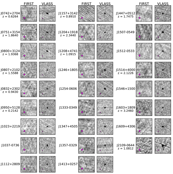
Figure 3: Cut-out images (30${}^{\prime\prime}\times 30^{\prime\prime}$) from FIRST (1.4 GHz; 1993-2011) and VLASS Epoch 1 (3 GHz; 2017–2019) of our sample. The synthesized beams (with typical major axis extents of approximately 5^′′ and 2.5^′′ for FIRST and VLASS, respectively) are shown as magenta ellipses in the lower left corner of each image.

To select AGN with variable radio emission, we considered both optical and infrared AGN selection techniques to capture both the unobscured and obscured populations. In the optical, we used the compilation of spectroscopically verified quasars from the Sloan Digital Sky Survey (SDSS; York et al. 2000) DR14 (Pâris et al., 2018) and found 52 candidate radio-variable quasars within $<1^{\prime\prime}$ of the VLASS position. Obscured AGN that have recently brightened in the radio were identified on the basis of their infrared colors using data from the Widefield Infrared Survey Explorer (WISE; Wright et al. 2010). We used the ”R90” diagnostic criteria from Assef et al. (2018), which were designed to identify AGN with 90% reliability. A total of 144 obscured AGN with variable radio emission were identified using the R90 catalog, of which 29 sources also met our optical selection criteria, making a total of 167 AGN associated with our manually-vetted FIRST/VLASS sample.

With the AGN associations confirmed, we selected a subset of sources with peak flux densities brighter than 3 mJy beam^-1 in VLASS. This selects a more reliable sample radio-variable AGN, since the implied spectral index between FIRST and VLASS would be steeper than $\nu^{2.5}$, thereby ruling out steady sources that are optically thick due to synchrotron self absorption (though free-free absorption is still a possibility). Following the 3 mJy cut, the final sample of radio-variable AGN contains 26 objects, and it is these that we consider in this paper. We provide an illustration of our selection criteria in Figure 2.

2.3 Source Properties

We summarize the basic properties of our sample in Tables 1 and 2. Of these 26 sources, 13 are selected from SDSS spectroscopy and the remaining 13 are obscured AGN selected based on the WISE criteria described in Section 2.2. The 13 optically-selected AGN are classified as broad-line quasars with redshifts in the range $0.2<z<3.2$. Shen et al. (2011) report bolometric luminosities of $\log(L_{\rm bol}/{\rm erg\,s^{-1}})\approx 45.2-46.8$ from SDSS spectroscopy, virial SMBH masses in the range $\log(M/{\rm M}_{\odot})\approx 8-9.7$, and Eddington ratios of 6–20% (consistent with radiatively efficient SMBH accretion; e.g. Heckman & Best 2014). All of our sources would have previously been classified as radio-quiet based on their upper limits in FIRST. The observed increase in radio flux between FIRST and VLASS suggests they are no longer in a radio-quiet state. Given the high VLASS radio luminosities ($L_{\rm 3\,GHz}=10^{40-42}\,\,{\rm erg}\,{\rm s}^{-1}$), our sources are now consistent with radio-loud quasars (Kellermann et al. 2016).

In Figure 3, we show image cut-outs from FIRST and VLASS. The 1$\sigma$ rms sensitivities of the FIRST and VLASS images are typically 0.15 mJy beam^-1 and 0.12 mJy beam^-1, respectively. The local rms noise level measured in each image is given in Table 2. The quality of the FIRST images is generally quite good. However, we note that one source in particular (J1157+3142) appears to have unusually poor image quality in the FIRST survey, making its classification as a variable AGN uncertain. We emphasize that while none of our sources met the formal detection threshold criteria ($F_{\rm peak}>1$ mJy) of the final release of the FIRST source catalog (Helfand et al., 2015), 12 sources have faint FIRST emission at the location of the VLASS source at the $3-3.6\sigma$ level (J1204+1918). We list sources with peak FIRST flux densities $>3\sigma$ as FIRST “detections” in Table 2.

Table 3: Summary of New Multiband VLA Observations

Source	Observing Date	Configuration	VLA Bands	Flux calibrator
(1)	(2)	(3)	(4)	(5)
J0742+2704	2019 Oct 03	A	L, S, C, X, Ku	3C147
J0807+2102	2019 July 23	BnA $\rightarrow$ A	L, S, C, X	3C286
	2019 Sept 19	A	X, Ku, K	3C138
J0832+2302	2019 July 23	BnA $\rightarrow$ A	L, S, C, X	3C286
	2019 Sept 19	A	X, Ku	3C138
J0950+5128	2019 July 23	BnA $\rightarrow$ A	L, S, C, X	3C286
	2019 Sept 19	A	X, Ku	3C138
J1037-0736	2019 Oct 13	A	L, S, C, X, Ku	3C286
J1204+1918	2019 Oct 11	A	L, S, C, X, Ku	3C286
J1208+4741	2019 Oct 11	A	L, S, C, X, Ku	3C286
J1246+1805	2019 Oct 11	A	L, S, C, X, Ku	3C286
J1254-0606	2019 Nov 01	A $\rightarrow$ D	L, S, C, X, Ku	3C286
J1413+0257	2019 Sept 23	A	L, S, C, X, Ku	3C286
J1447+0512	2019 Sept 23	A	L, S, C, X, Ku	3C286
J1546+1500	2019 Sept 23	A	L, S, C, X, Ku	3C286
J1603+1809	2019 Sept 23	A	L, S, C, X, Ku	3C286
J2109-0644	2019 Sept 10	A	L, S, C, X, Ku	3C48

Note. — Column 1: Source name. Column 2: Observing date(s). Column 3: VLA configuration. Column 4: VLA band, defined as follows: L: 1–2 GHz, S: 2–4 GHz, C: 4–8 GHz, X: 8–12 GHz, Ku: 12–18 GHz, K: 18–26 GHz. Column 5: Flux density calibrator. We note that the calibrator 3C48 is currently experiencing an ongoing flaring event. As a result, the absolute flux uncertainty of sources calibrated against this source will be increased. We therefore assume a conservative flux uncertainty of 20% for all sources using 3C48 as the primary flux calibrator. All other flux calibrators are expected to provide an absolute uncertainty of 3% Perley & Butler (2013).

The VLASS QuickLook image cut-outs shown in Figure 3 highlight the radio variability of our sources on timescales of $\sim 1-2$ decades as well as their compactness on $\sim$arcsecond scales. Some of the VLASS QuickLook images suffer from strong imaging artifacts, such as prominent sidelobes due to insufficient cleaning and/or the presence of residual phase errors. This is due to the rough nature of the QuickLook images, which we emphasize are not the final VLASS survey products. Despite the known limitations of the QuickLook images, we find the peak VLASS flux densities of our compact sources to typically be consistent with our independent VLA follow-up imaging at $S$-band (see Section 4.2 for a discussion of source variability at $S$ band). Thus, our study supports the viability of the use of VLASS QuickLook images for science as long as users take the known limitations into account.

3 VLA Follow-up Data

We performed high-resolution, multiband VLA observations for 14/26 candidate variable AGN through project 19A-422 (PI: Gregg Hallinan). These observations took place from July 23 – October 13, 2019, primarily during the VLA A configuration. For each source, the observations at $L$ (1–2 GHz), $S$ (2–4 GHz), $C$ (4–8 GHz), and $X$ (8–12 GHz) band were performed within a single scheduling block (SB) no longer than 2.75 hr, and we therefore refer to these observations as “quasi-simultaneous” in nature.

In addition to the 1–12 GHz observations, the majority of our sources also have quasi-simultaneous data at Ku (12–18 GHz) band. Because a preliminary analysis of our first three pilot sources (J0807+2102, J0832+2302, and J0950+5128) showed rising fluxes at high frequencies, we modified our observing strategy to add higher frequency $Ku$-band observations (12–18 GHz) for the remaining sample, and returned later to our three pilot sources on September 19, 2019 to repeat the $X$-band observations and add $Ku$ band. We discuss the X-band variability on $\sim$weeks timescale for these three sources in Section 4.2. Finally, for the pilot source J0807+2102 with the most optically-thick spectrum, we added a $K$-band (18-26 GHz) observation. The dates and frequencies of all our VLA observations are given in Table 3.

3.1 Calibration and Imaging

We calibrated our data using the scripted VLA calibration pipeline for the Common Astronomy Software Applications (CASA) package (McMullin et al., 2007) version 5.3.0. In order to ensure the use of an optimal calibration solution interval for each band, the pipeline was run separately for each band of each SB.

Imaging and self-calibration were performed in CASA 5.6.0 following standard heuristics for widefield, broadband VLA data. We used the TCLEAN task to produce a full field-of-view image at each band and employed the $w$-projection algorithm (Cornwell et al., 2005) to correct for non-coplanar baselines. To avoid bandwidth smearing over the large fractional bandwidths of our observations, deconvolution was performed using the MTMFS (multi-term, multi-frequency synthesis) algorithm (Rau & Cornwell, 2011). We adopted a Briggs weighting scheme (Briggs, 1995) with a robust parameter between -0.5 and 0.5 to achieve the best compromise among sidelobe levels, resolution, and sensitivity given the quality of the $uv$-coverage and resulting point-spread function (PSF) of each dataset.

3.2 VLITE

Commensal low-frequency ($<$1 GHz) data were also recorded during our VLA follow-up campaign. This commensal system, known as the VLA Low-band Ionosphere and Transient Experiment (VLITE; Clarke et al. 2016; Polisensky et al. 2016), records data at 340 MHz simultaneously with regular VLA observing programs. During our VLA observations, commensal VLITE data with a maximum of 18 antennas were recorded.

VLITE data are automatically calibrated and imaged through an analysis pipeline based on the Obit (Cotton, 2008) data reduction package. The VLITE pipeline images from our snapshot observations typically achieve a 1$\sigma$ depth of 3 mJy beam ^-1 and a maximum angular resolution of $\approx 5^{\prime\prime}$. We visually inspected all VLITE imaging pipeline products and found that none of our sources was detected, as expected given their curved or flat radio SEDs. We discuss constraints on the radio SEDs and underlying emission mechanisms using the upper limits from VLITE in Section 4.3.

4 Results

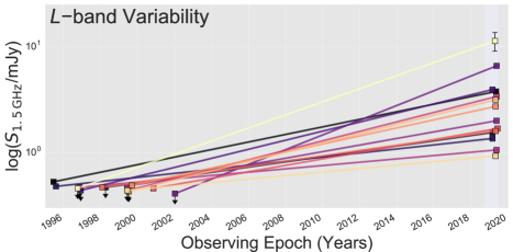
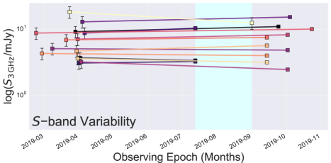
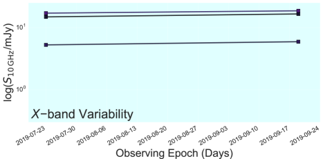
Figure 4: Radio flux variability at $L$, $S$, and $X$ band. Two observing epochs are shown for each band. At $L$ band, we show the flux measurements or upper limits from FIRST (1993–2011) and the flux densities from our 2019 JVLA follow-up observations. At $S$ band, we show the flux densities from VLASS Epoch 1.2, which were observed in early 2019, and the $S$-band flux densities from our follow-up observations taken a few months later. All of the VLASS $S$-band measurements are shown with a conservative 20% flux uncertainty (Lacy et al., 2020). The large uncertainty (20%) in the flux of a single object (J2109-0644) is apparent at both $L$ and $S$ band in our 2019 observations; we discuss limitations of the absolute flux scale calibration for this source in Section 3. At $X$ band, only 3 sources (J0807+2102, J0832+2302, and J0950+5128), which have two epochs of $X$-band observations, are shown (see Sections 3 and 4.2).

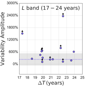
Figure 5: Variability amplitude as a function of time from the dual-epoch observations at $L$ and $S$ band shown in Figure 4. In the left panel, the variability amplitude is shown as the percent change in flux between FIRST and our 1.5 GHz follow-up observations, or $(F_{\rm FIRST}-F_{1.5\,\rm GHz})/F_{\rm FIRST}$. In the right panel, the variability amplitude is the percent change in flux between VLASS and our 3 GHz follow-up observations, or $(F_{\rm VLASS}-F_{3\,\rm GHz})/F_{\rm VLASS}$. The dashed lines indicate the median variability amplitude at each band and the gray shaded regions denote the weighted 1$\sigma$ standard deviations. The large errors on the $S$-band variability amplitudes are dominated by the conservative 20% uncertainty in the flux densities measured from the VLASS Epoch 1 QuickLook images (Lacy et al., 2020).

Table 4: Radio Spectral Modeling Parameters

Source	$\theta_{\rm max}$	Linear Size	$\nu_{\rm peak}$	$\nu_{\rm peak,\,rest}$	$\chi_{\rm red,\,PL}^{2}$	$\chi_{\rm red,\,CPL}^{2}$	$q$	$\alpha_{\rm thick}$	$\alpha_{\rm thin}$
	(arcsec)	(pc)	(GHz)	(GHz)
(1)	(2)	(3)	(4)	(5)	(6)	(7)	(8)	(9)	(10)
J0742+2704	$<$0.17	$<$1193	8.6	14.0	107.75	9.23	$-0.65\pm 0.09$	1.59$\pm$0.10	$-0.62\pm 0.17$
J0807+2102	$<$0.11	$<$956	21.9	56.2	67.53	35.97	$-0.36\pm 0.16$	1.25$\pm$0.11	$\cdots$
J0832+2302	$<$0.17	$<$1379	11.4	22.1	39.49	3.96	$-0.40\pm 0.06$	1.36$\pm$0.11	$\cdots$
J0950+5128	$<$0.16	$<$575	13.2	16.0	34.53	5.78	$-0.34\pm 0.07$	1.43$\pm$0.10	$\cdots$
J1037-0736	$<$0.17	$\cdots$	6.2	$\cdots$	74.88	5.74	$-0.54\pm 0.07$	1.35$\pm$0.11	$-0.44\pm 0.17$
J1204+1918	$<$0.16	$<$1341	4.6	15.5	132.82	3.99	$-0.75\pm 0.06$	1.27$\pm$0.10	$-1.16\pm 0.17$
J1208+4741	$<$0.12	$<$1006	5.6	11.8	89.17	6.44	$-0.58\pm 0.08$	1.32$\pm$0.11	$-0.61\pm 0.16$
J1246+1805	$<$0.13	$\cdots$	9.0	$\cdots$	46.30	2.52	$-0.40\pm 0.05$	1.28$\pm$0.10	$-0.09\pm 0.17$
J1254-0606	$<$0.15	$\cdots$	6.6	$\cdots$	236.24	2.25	$-1.09\pm 0.04$	2.57$\pm$0.10	$-1.16\pm 0.17$
J1413+0257	$<$0.21	$\cdots$	6.4	$\cdots$	215.22	1.96	$-1.02\pm 0.04$	2.20$\pm$0.10	$-1.22\pm 0.17$
J1447+0512	$<$0.18	$<$1562	2.6	7.3	43.75	29.84	$-0.34\pm 0.17$	$\cdots$	$-0.45\pm 0.17$
J1546+1500	$<$0.16	$\cdots$	4.8	$\cdots$	43.58	11.91	$-0.38\pm 0.10$	0.84$\pm$0.10	$-0.29\pm 0.17$
J1603+1809	$<$0.17	$<$1308	8.1	34.6	109.40	0.23	$-0.66\pm 0.01$	1.76$\pm$0.10	$-0.47\pm 0.17$
J2109-0644	$<$0.17	$<$1423	6.5	13.5	13.74	9.94	$-0.18\pm 0.09$	0.15$\pm$0.11	$-0.41\pm 0.16$

Note. — Column 1: Source name. Column 2: Angular size upper limit from the highest resolution VLA data available. Column 3: Linear size upper limit for sources with known redshifts. Column 4: Spectral peak (or “turnover”) frequency ($\nu_{\rm peak}$) from a fit to a curved power-law model. Column 5: Same as Column 4, but in the rest frame for sources with known redshifts. Column 6: Reduced chi squared value for the fit to a simple power-law model. Column 7: Reduced chi squared value for the fit to a curved power-law model. Column 8: Spectral curvature parameter, $q$, from a fit to a curved power-law model. Column 9: The optically-thick spectral index, $\alpha_{\rm thick}$, estimated by a power-law fit to the two lowest frequency VLA bands ($L$ and $S$ band). The uncertainties were calculated using standard propagation of errors. We required $\nu_{\rm peak}>$4 GHz to estimate $\alpha_{\rm thick}$. Column 10: Estimates of the optically-thin spectral index, $\alpha_{\rm thin}$ (and the corresponding uncertainties), from a power-law fit to the two highest frequency VLA bands (either $X$ and Ku band or Ku and $K$ band) above $\nu_{\rm peak}$. We required quasi-simultaneous VLA measurements in at least two bands above $\nu_{\rm peak}$ to estimate $\alpha_{\rm thin}$.

4.1 Radio flux densities and Morphologies

Source flux and shape measurements for the VLA data above 1 GHz were made using the CASA IMFIT task and are reported in Table 6. For the majority of sources, the flux errors include a standard 3% uncertainty in the absolute flux scale (Perley & Butler, 2017), added in quadrature with the flux error reported by IMFIT. Due to scheduling limitations, one of our sources (J2109$-$0644) was observed using 3C48 as the flux calibrator. Because 3C48 is currently flaring, we conservatively report a flux uncertainty of 20% for each measurement of J2109$-$0644 following current NRAO guidelines.

Our sources are characterized by compact ($\lesssim$0.1^′′) radio continuum emission over the full frequency range of our VLA study, which provides a maximum angular resolution of $\theta_{\rm max}\lesssim 0.1^{\prime\prime}$ (for the Ku-band/A-configuration data). This corresponds to an upper limit on the intrinsic linear source sizes that is $<1$ kpc.

4.2 Constraints on Variability

We illustrate the flux variations of our sample at $L$ and $S$ band over two epochs probing two different timescales in Figures 4 and 5. We also show the variability at $X$-band for the 3 sources (J0807+2102, J0832+2302, and J0950+5128) in our sample with a gap of several weeks between observations from 1–12 GHz ($L$, $S$, $C$, and $X$ band) and 12–18 GHz (Ku band). Tables 2 and 3 provide additional details on the observing dates of the data from FIRST, VLASS, and our new multiband JVLA follow-up observations.

At $L$-band, the two epochs shown in the top panel of Figure 4 are from the FIRST survey (with observing dates ranging from 1995 to 2002 for our sample) and our 2019 JVLA follow-up study. The $L$-band source flux densities from our new JVLA observations range from $\sim 1-11$ mJy. Thus, compared to the FIRST flux measurements made 17 to 24 years earlier, our sources have $L$-band flux densities that have increased dramatically by factors of $\sim$2–25. The left panel of Figure 5 shows the variability amplitude at $L$ band between FIRST and our 2019 observations for each source. The weighted median value is $\sim$200%. However, we emphasize that since half of our sources remain undetected below the 3$\sigma$ level in FIRST, this is likely to be a lower limit. Thus, the true $L$-band variability amplitude on timescales of $\sim$1–2 decades could be even higher.

At $S$-band, the two observing epochs shown in Figure 4 span a much narrower range of time ($\sim$months) compared to the variability timescale constraints at $L$ band ($\sim$decades). The $S$-band flux densities between our JVLA follow-up observations and VLASS are approximately constant over timescales of 3–7 months. This is clearly illustrated in the right panel of Figure 5, which shows the $S$-band variability amplitude has a median value of $\sim$15%. Thus, our follow-up JVLA $S$-band data are typically in good agreement within the current $\sim$20% flux uncertainties of VLASS. We note that the most substantial outlier in the right panel of Figure 5 is the source J2109-0644, which as discussed in Section 3 may have unusually large absolute flux errors due to the variability of the flux calibrator.

At $X$-band, the two observing epochs shown in Figure 4 for J0807+2102, J0832+2302, and J0950+5128 span an even narrower range of time ($\sim$weeks) compared to the variability timescale constraints at $L$ and $S$ band. The $X$-band flux densities are roughly constant, although all 3 sources exhibit a slight increase in flux of $\sim$10% over a period of 58 days. Although an increase in flux density of this magnitude could be due to the evolution of a nascent jet (see Section 5), the presence of residual errors in the absolute flux scale of similar magnitude cannot be entirely ruled out. This is because the first epoch of $X$-band observations was taken during the move from the hybrid BnA configuration to the standard A array, which lead to poor PSF quality that ultimately posed challenges for self calibration and deconvolution (see Section 3). Nevertheless, we conclude that the $X$-band flux densities are in close enough agreement to justify the inclusion of the observations above 12 GHz in our radio SED analysis.

Although our time domain assessment is currently crude and would benefit from higher-cadence monitoring in the future, we conclude that our sources are characterized by large amplitude (2–25X) variability at $L$ band on timescales 1–2 decades, but maintain roughly constant flux densities over timescales of a few months at $S$ band. Thus, the typical variability timescale, $\tau_{\rm var}$, likely falls in the range of $3-7$ months $<\tau_{\rm var}<17-24$ years. We discuss implications of these constraints on the origin of the radio variability in Section 5.

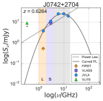
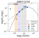
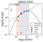
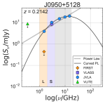
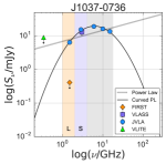
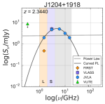
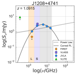
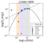
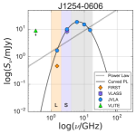
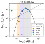
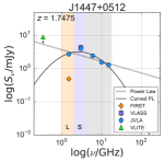
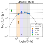
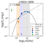
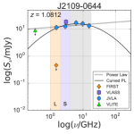
Figure 6: Broadband radio SEDs showing our quasi-simultaneous multiband JVLA imaging (blue circles), the VLASS detection (purple squares), FIRST upper limit or 3$\sigma$ detection (orange diamonds), and VLITE upper limit (green triangles). For each source, two models based on the quasi-simultaneous JVLA data are shown: a standard non-thermal power-model (dotted line) and a curved power-law model (solid line).

4.3 Quasi-simultaneous Radio SEDs

In Figure 6, we show the radio SEDs of the 14 sources from our sample with quasi-simultaneous VLA observations from 1–18 GHz. The radio SEDs have peaked spectral shapes with varying degrees of curvature easily discernible by eye. This indicates the presence of an underlying absorption mechanism, such as synchrotron self absorption (SSA) or free-free absorption (FFA), as is commonly associated with compact radio sources (Callingham et al. 2017; Collier et al. 2018).

4.3.1 Radio SED Modeling

To quantify the location of the spectral peak and degree of curvature, we performed least squares fits to the quasi-simultaneous VLA data above 1 GHz using two basic synchrotron emission models:

1. A standard non-thermal power-law model defined by $S_{\nu}=a\nu^{\alpha}$, where $S_{\nu}$ is the flux at frequency $\nu$, $a$ represents the amplitude, and $\alpha$ is the spectral index.

2. A curved power-law model defined by $S_{\nu}=a\nu^{\alpha}e^{q(\ln\nu)^{2}}$, where $q$ represents the degree of spectral curvature (the breadth of the peak of the radio SED). The $q$ parameter is defined by $\nu_{\rm peak}=e^{-\alpha/2q}$, where $\nu_{\rm peak}$ is the turnover frequency. Significant spectral curvature is typically defined as $|q|\geq 0.2$ (Duffy & Blundell, 2012; Callingham et al., 2017).

We note that our use of the curved power-law model is phenomenological in nature. More physically motivated spectral curvature models, such as SSA or FFA (or models with contributions from multiple electron populations; Tingay et al. 2015), require more than 3 free parameters, and thus have only a few degrees of freedom given the number of bands (typically 5; see Table 3) available for each source.

We summarize our spectral modeling analysis in Table 4. Based on the reduced chi-square values provided in this table, a curved power-law model provides a better fit compared to a simple power-law model for all sources. The observed spectral turnover frequencies for our sources range from 2.5–22.7 GHz, with a median value of $\nu_{\rm peak}=6.6$ GHz. For sources with measured redshifts, the corresponding rest-frame turnover frequencies lie in the range of $\nu_{\rm peak,\,rest}=6.8-58.1$ GHz. Likewise, the values of $q$ from the curved power-law fits span the range $0.18<|q|<1.09$ confirming that essentially all are strongly curved. The exception is J2109-0644, which is only marginally below the formal limit of $|q|>0.2$, and the VLITE upper limit at 340 MHz supports a curved, not flat, radio SED.

In Table 4, we also provide the optically-thick and optically-thin spectral index values ($\alpha_{\rm thick}$ and $\alpha_{\rm thin}$) below and above the turnover frequency, respectively. We estimated $\alpha_{\rm thick}$ by fitting a power-law model to the quasi-simultaneous flux densities at the two lowest frequency VLA bands ($L$ and $S$ band) below the turnover frequency. Estimates for $\alpha_{\rm thick}$ are only provided for sources with $\nu_{\rm peak}>4$ GHz (spectral peaks above the VLA $S$ band). For $\alpha_{\rm thin}$, we performed a power-law fit to the quasi-simultaneous flux densities at the two highest frequency VLA bands (either $X$ and Ku band or Ku and $K$ band above the turnover frequency. We required the quasi-simultaneous VLA data to include at least two independent bands above the turnover frequency to estimate $\alpha_{\rm thin}$. The uncertainties in $\alpha_{\rm thick}$ and $\alpha_{\rm thin}$ provided in Table 4 were calculated using standard propagation of errors.

Based on the radio spectral modeling analysis described here, we conclude that the radio SEDs of our sources are best represented by curved power-law models (as opposed to flat power-law models lacking curvature), thus supporting the presence of significant spectral curvature. In a future study, we will incorporate new data from forthcoming VLA and Giant Metre-wave Radio Telescope (GMRT) observations spanning a broader frequency range (the full contiguous frequency range of the VLA from 1–50 GHz and deep measurements below 1 GHz using the VLA and GMRT). This will enable a more rigorous radio SED modeling analysis that will allow us to test whether SSA of FFA are responsible for the observed spectral curvature (Mhaskey et al. 2019a, b).

4.3.2 Radio Color-color Diagram

In Figure 7, we show our sources on a radio color-color diagram ($\alpha_{\rm thick}$ vs. $\alpha_{\rm thin}$). All of our sources reside in the second quadrant of this figure, which characterizes peaked radio spectral shapes indicative of an underlying absorption mechanism commonly associated with source compactness due to youth and/or confinement by an external medium (O’Dea 1998; O’Dea & Saikia 2020; Orienti 2016). Most of our sources also meet the more strict selection criteria for peaked-spectrum radio sources from Callingham et al. (2017) of $\alpha_{\rm thick}>0.1$ and $\alpha_{\rm thin}<-0.5$).

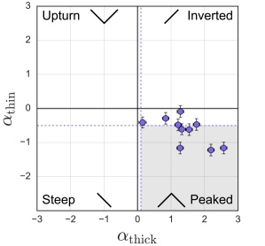
Figure 7: Radio color-color diagram for sources with well-defined optically-thick and optically-thin spectral indices ($\alpha_{\rm thick}$ and $\alpha_{\rm thin}$, respectively). Details on the calculation of $\alpha_{\rm thick}$ and $\alpha_{\rm thin}$ are provided in Section 4.3 and Table 4. The gray shaded region highlights the selection criteria for peaked-spectrum radio sources from Callingham et al. (2017) of $\alpha_{\rm thick}>0.1$ and $\alpha_{\rm thin}<-0.5$.

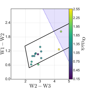
Figure 8: WISE infrared color-color diagrams (W1 = 3.4$\mu$m, W2 = 4.6$\mu$m, and W3 = 12$\mu$m) in Vega magnitudes. The black wedge defines the color space for luminous AGN in WISE defined by Mateos et al. (2012). The shaded region bounded by the dashed diagonal line, defined as $(W1-W2)+1.25(W2-W3)>7$, identifies extremely red sources likely to be heavily obscured, luminous AGN (Lonsdale et al., 2015; Patil et al., 2020). The points in the left- and right-hand plots are colorized by the radio spectral curvature parameter ($q$) and the optically-thick radio spectral index ($\alpha_{\rm thick}$), respectively.

Our sources have optically-thick spectral index constraints that are consistent with SSA, though improved spectral coverage at low frequencies ($<1$ GHz) will ultimately be needed (Callingham et al. 2015; Collier et al. 2018; Mhaskey et al. 2019a, b; Keim et al. 2019). The identification of FFA associated with any of the newly radio-loud AGN in our sample would be of particular interest in the context of galaxy evolution since simulations have shown that it may arise from jet-ISM interactions (Bicknell et al., 1997, 2018). Such jet-ISM interactions may subsequently influence the ambient star formation rate and/or efficiency, as argued by recent observational studies in low-redshift galaxies (Morganti et al. 2013; Nyland et al. 2013; Mukherjee et al. 2018; Husemann et al. 2019; Jarvis et al. 2019; Ruffa et al. 2019).

Table 5: Infrared Source Properties

Source	W1	W2	W3	W4	$\log(L_{6\mu\rm m,\,rest})$
	(mag)	(mag)	(mag)	(mag)	(erg s-1)
(1)	(2)	(3)	(4)	(5)	(6)
J0742+2704	14.42$\pm$0.03	13.68$\pm$0.04	11.25$\pm$0.15	$\cdots$	45.05
J0751+3154	15.98$\pm$0.06	14.86$\pm$0.07	$\cdots$	$\cdots$	46.24
J0800+3124	15.91$\pm$0.05	14.70$\pm$0.07	12.26$\pm$0.41	$\cdots$	46.30
J0807+2102	15.91$\pm$0.06	14.72$\pm$0.07	11.64$\pm$0.25	$\cdots$	46.14
J0832+2302	13.84$\pm$0.03	12.46$\pm$0.03	9.45$\pm$0.04	7.21$\pm$0.11	46.07
J0950+5128	13.43$\pm$0.02	12.80$\pm$0.03	10.40$\pm$0.08	8.22$\pm$0.25	44.13
J1023+2219	15.85$\pm$0.05	14.77$\pm$0.07	11.32$\pm$0.20	8.47$\pm$0.34	$\cdots$
J1037-0736	14.82$\pm$0.03	13.83$\pm$0.04	11.22$\pm$0.16	$\cdots$	$\cdots$
J1112+2809	16.33$\pm$0.07	15.40$\pm$0.10	$\cdots$	$\cdots$	$\cdots$
J1157+3142	14.98$\pm$0.03	13.82$\pm$0.04	11.26$\pm$0.16	8.62$\pm$0.41	45.40
J1204+1918	16.07$\pm$0.06	15.17$\pm$0.09	12.08$\pm$0.33	8.85$\pm$0.41	46.54
J1208+4741	16.16$\pm$0.06	15.18$\pm$0.07	12.70$\pm$0.43	$\cdots$	45.26
J1246+1805	16.53$\pm$0.07	15.43$\pm$0.10	12.72$\pm$0.47	$\cdots$	$\cdots$
J1254-0606	15.92$\pm$0.05	14.65$\pm$0.06	10.35$\pm$0.06	7.83$\pm$0.16	$\cdots$
J1333-0349	15.34$\pm$0.04	14.35$\pm$0.05	11.99$\pm$0.25	$\cdots$	$\cdots$
J1347+4505	15.22$\pm$0.04	13.87$\pm$0.03	10.82$\pm$0.09	$\cdots$	$\cdots$
J1357-0329	13.87$\pm$0.03	12.77$\pm$0.03	9.87$\pm$0.05	7.39$\pm$0.10	$\cdots$
J1413+0257	18.14$\pm$0.25	16.11$\pm$0.17	11.65$\pm$0.17	8.94$\pm$0.32	$\cdots$
J1447+0512	16.20$\pm$0.06	15.14$\pm$0.07	$\cdots$	$\cdots$	46.03
J1507-0549	15.97$\pm$0.06	15.12$\pm$0.10	12.04$\pm$0.29	$\cdots$	$\cdots$
J1512-0533	16.66$\pm$0.08	15.19$\pm$0.10	12.43$\pm$0.39	9.10$\pm$0.47	$\cdots$
J1514+4000	16.22$\pm$0.05	15.54$\pm$0.08	12.13$\pm$0.19	9.53$\pm$0.52	46.21
J1546+1500	15.97$\pm$0.05	14.90$\pm$0.07	$\cdots$	$\cdots$	$\cdots$
J1603+1809	16.10$\pm$0.05	15.47$\pm$0.09	12.59$\pm$0.48	$\cdots$	47.05
J1609+4306	16.38$\pm$0.05	15.41$\pm$0.08	13.12$\pm$0.43	9.62$\pm$0.48	$\cdots$
J2109-0644	15.14$\pm$0.04	14.07$\pm$0.04	11.21$\pm$0.17	8.22$\pm$0.31	45.71

Note. — Column 1: Source name. Columns 2-5: WISE W1 (3.4$\mu$m), W2 (4.6$\mu$m), W3 (12$\mu$m), and W4 (22$\mu$m) band magnitudes and errors from the AllWISE source catalog (Cutri & et al., 2013). Column 6: Estimated rest-frame 6$\mu$m luminosity extrapolated from a power-law fit to the AllWISE photometry.

4.3.3 Infrared Color-Color Diagram

In Figure 8, we show the distribution of the 14 sources from our multiband VLA follow-up campaign in WISE infrared color space ($W2-W3$ vs. $W1-W2$). A summary of the infrared properties of our sources is provided in Table 5. All but one these sources meet the infrared color selection criteria for obscured quasars defined by Mateos et al. (2012). The single exception is J1603+1809, which is identified as a Type 1 quasar in SDSS, but does not meet the WISE AGN selection criteria of the Assef et al. (2018) R90 catalog.

We also highlight the region occupied by extremely red and powerful AGN defined by $(W1-W2)+1.25(W2-W3)>7$ (Lonsdale et al., 2015) in Figure 8. Sources with such extreme mid-infrared colors are believed to be heavily obscured, ultra-luminous quasars. Of our 14 sources one source, J1413+0257, meets the Lonsdale et al. (2015) selection criteria. Although this source currently lacks redshift information, Patil et al. (2020) reported redshifts in the range $0.4<z<3.0$ (with a median value of $z\sim 1.5$) and luminosities of $\log(L_{\rm bol}/{\rm L}_{\odot})\sim 11.7-14.2$ for a sample of quasars in the Lonsdale et al. (2015) color space also harboring compact radio sources.

Finally, we use Figure 8 to investigate possible relationships between the WISE colors and two key parameters from our radio spectral modeling: the spectral curvature parameter, $q$, and the optically-thick spectral index, $\alpha_{\rm thick}$. Qualitatively, Figure 8 suggests an association between both a higher degree of spectral curvature (a narrower spectral peak) and $\alpha_{\rm thick}$ values for redder sources.

Previous studies have reported evidence for a connection between quasar reddening and radio jet properties possibly arising from hierarchical SMBH-galaxy co-evolution (Georgakakis et al. 2012; Glikman et al. 2012; Klindt et al. 2019; Patil et al. 2020; Fawcett et al. 2020; Rosario et al. 2020). In such a scenario, a quasar may transition to a radio-loud phase following a gas-rich merger and subsequent change in SMBH accretion state and/or spin conducive to jet formation. In a future study, we will investigate this possibility in more detail by constraining the origin of the reddening in our sample through optical and infrared SED modeling. Ultimately, observations of a larger sample will be needed to more firmly establish the relationship between the infrared colors and radio SED properties in young radio quasars.

5 Origin of the Radio Variability

In this section, we consider different scenarios for the origin of the radio variability in our sample based on the current constraints on source luminosities, radio spectral shapes, and observed variability properties (amplitude and timescale). Regarding the variability properties, we emphasize that our cadence is currently very sparse, with only three observations (FIRST, VLASS, and our multiband follow-up) spaced by roughly six months and two decades. Although this is clearly insufficient to infer the full character of the variability, we assume that the simple flux ratios provide a provisional measure of the variability on each timescale (see Section 4.2). Future observations will yield a richer cadence that will further clarify the variability on different timescales.

5.1 Plasma Propagation Effects

Radio waves traveling through an inhomogeneous plasma may be modulated by scattering or lensing phenomena. This may lead to variations in the observed properties of compact sources, such as flat-spectrum radio AGN. Physical mechanisms responsible for such propagation effects include interplanetary scintillation (IPS; Morgan et al. 2018, and references therein), interstellar scintillation (ISS; Jauncey et al. 2016, and references therein), and extreme scattering events (ESEs; Fiedler et al. 1987).

IPS arises from turbulence in the solar wind plasma and leads to rapid flux variability on timescales of roughly seconds in low-frequency ($\sim$100 MHz) radio observations. Although IPS has proven to be a powerful tool for identifying compact radio AGN in low-frequency surveys (e.g. Chhetri et al. 2018), it is not compatible with the variability timescales and amplitudes observed in our sample above 1 GHz.

ISS is caused by the refraction or diffraction of radio waves emitted by a microarcsecond-scale source as they pass through fluctuations in the plasma density and/or magnetic field of the ionized ISM in our Galaxy (Stanimirović & Zweibel, 2018). This leads to variable radio emission on timescales of hours to days with a strong dependence on galactic latitude.

Observational manifestations of ISS (i.e. variability amplitude and timescale) depend on the Galactic free electron density along a particular line of sight as well as the observing frequency. The distribution of our sources in Galactic latitude is approximately flat (Figure 1), arguing against ISS as the main driver of the observed radio variability. As a more quantitative test of an ISS variability origin for each source, we computed the critical frequency, $\nu_{0}$, below which the modulation due to scintillation is in the strong regime. At the positions of our sources we find $\nu_{0}$ = 7.1–11 GHz. For observations at $\nu$ = 1.5 GHz, we are therefore well within the strong scattering regime and the equations from Section 3.2 of Walker (1998) apply. For point sources in this limit that are experiencing refractive scintillation, the expected flux modulation at 1.5 GHz is m = ($\nu_{0}$/$\nu$)^17/30 $\sim$ 30–40%. This modulation is expected to occur on a timescale of $t_{r}\sim 2(\nu_{0}/\nu)^{11/5}$ hours $\sim$ 2–7 days. This stands in sharp contrast to the observed modulations of $\gtrsim$100% to $\gtrsim$2500% occurring on observed timescales of months to decades for our sources, thus ruling out refractive ISS as the origin of the radio variability in our sample.

Diffractive ISS, which is associated with interference, leads to variability over an even narrower bandwidth and shorter timescale, making it considerably less plausible than refractive ISS. The fluctuations (of order unity) last for only $\sim$0.1 – 0.3 hours. Furthermore, at 1.5 GHz, any diffractive ISS would be decorrelated over a bandwidth of $\delta\nu\sim 1-5$ MHz. This modulation would thus be washed out by averaging over a single VLA frequency channel.

Another plasma lensing phenomenon known to produce radio variability is that of ESEs (Fiedler et al. 1987). In this case, refractive defocusing by the transverse passage of a discrete, high-density plasma lens in front of a compact radio source leads to a reduction of flux with a characteristic U-shaped light curve (Clegg et al. 1998; Bannister et al. 2016). The variability amplitude (a reduction in emission of $\lesssim 50$%) and timescale (weeks to months) for an ESE are typically larger in magnitude compared to ISS. At least one case of an ESE with a threefold modulation in flux in the centimeter-wave radio regime is known (Bannister et al., 2016). This overlaps with the lower range in variability amplitude of our sample. However, we note that the timescale for the high-amplitude radio variability reported in Bannister et al. (2016) is a few months. This stands in sharp contrast to our sources, which vary on decades-long timescales but are steady over periods of a few months.

While we cannot totally rule out contributions to the observed radio variability by serendipitous propagation effects, we find such scenarios to be unlikely given inconsistencies with the high variability amplitudes and long timescales observed in our sample.

5.2 Supernovae and Gamma-Ray Bursts

Variable radio emission may be associated with supernovae and gamma-ray bursts (GRBs), arising from collimated outflows of high-mass supernovae and compact object mergers (neutron stars and stellar-mass black holes) (Weiler et al., 2002; Woosley & Bloom, 2006; Berger, 2014). However, the high luminosities of our sources (Table 2) rule out the possibility of a radio supernova afterglow (Palliyaguru et al., 2019) as a progenitor scenario. Regarding the possibility of radio variability associated with a GRB origin, we note that our sources are on par with, or more luminous than, on-axis GRBs, which have peak luminosities of $\sim 10^{31}$ erg s^-1 Hz^-1 (Chandra & Frail, 2012). However, the typical variability timescale of radio emission associated with GRBs is around 1–2 weeks (Pietka et al., 2015). This is considerably shorter than the variability timescale constraints for our sources ($>$ a few months), thus ruling-out the possibility of a GRB progenitor.

5.3 Tidal Disruption Events

Tidal disruption events (TDEs; e.g., Komossa 2015, and references therein) occur when a star passes within the tidal radius of a SMBH and is ripped apart and partially accreted onto the SMBH. This leads to a multi-wavelength flare, which in some cases includes the production of radio continuum emission associated with non-thermal jets or thermal outflows (van Velzen et al. 2011, 2016; Anderson et al. 2020). The most radio luminous known TDE, Swift J1644+57, peaked at $\sim$10³²  erg s^-1 Hz^-1 (Eftekhari et al., 2018), which is roughly in line with the radio luminosities of our sources. In addition, recent studies have suggested that TDEs may be responsible for triggering a significant fraction of the changing-look AGN population, particularly at $z>2$ (Padmanabhan & Loeb, 2020). Because more massive black holes have weaker tidal fields near their event horizons, TDEs for main sequence stars become increasingly rare above a critical mass of about ($10^{8}$ M_⊙, Hills 1975). Main sequence stars that approach SMBHs above this limiting mass are “swallowed whole” (MacLeod et al. 2012), and thus do not lead to the production of an electromagnetic flare. As shown in Table 1, the available SMBH mass estimates of our sources typically exceed $10^{8}$ M_⊙, suggesting that TDEs are unlikely progenitors for the majority of our sources.

On the other hand, evolved stars with large diffuse envelopes, such as red giants, are in principle susceptible to tidal disruption by a SMBH with $M_{\rm SMBH}>10^{8}$ M_⊙. However, such events are expected to be rare due to the relatively short duration of the red giant phase compared to main sequence lifetimes. Recent studies have also argued that TDEs of giant stars by SMBHs with masses above $10^{8}$ M_⊙ may be less luminous than TDEs associated with lower-mass SMBHs (Bonnerot et al. 2016).

Although TDEs may provide a plausible mechanism for driving the extreme radio variability in some of our sources, the current literature consensus is that TDEs with powerful relativistic jets are rare (e.g., van Velzen et al. 2018), composing only a few percent of the known TDE population (Alexander et al. 2020, and references therein). Thus, based on the high radio luminosities and SMBH masses of our sample, as well as the low space density of radio-loud TDEs, we conclude that the radio variability in our sources is most likely not associated with TDEs.

5.4 Intrinsic AGN Variability

While the large-scale lobes of radio galaxies are believed to remain steady over Myr to Gyr timescales (Blandford et al., 2019), intrinsic radio variability on human timescales (days to years) is common among AGN with compact ($<1$ kpc) jets such as blazars (Lister, 2001), unbeamed radio quasars/galaxies with young jets (Torniainen et al., 2005; Orienti & Dallacasa, 2020; Kunert-Bajraszewska et al., 2020), the cores of FRI/FRII (Fanaroff & Riley, 1974) radio galaxies (Chatterjee et al., 2011; Maccagni et al., 2020), and low-luminosity AGN (Mundell et al., 2009; Brunthaler et al., 2005). Although the physics of the intrinsic variability of compact AGN jets remains an unsolved problem, plausible mechanisms include the propagation of shocks along the jet (Marscher & Gear, 1985) and changes in the SMBH accretion properties such as accretion disk instabilities (Czerny et al., 2009; Janiuk & Czerny, 2011) or accretion state changes (Koay et al., 2016; Wołowska et al., 2017). In addition to variability mechanisms directly related to accretion, radio variability may also arise from the jet itself owing to jet reorientation and the evolution of a young, expanding jet (e.g. Kunert-Bajraszewska et al. 2020; An et al. 2020). We focus on accretion-driven radio variability in this section and discuss jet reorientation and youth in Sections 5.5 and 5.6.

Each radio variability scenario described above is characterized by differences in variability amplitude level, as well as temporal and spectral evolution. Thus, distinguishing amongst them is best accomplished through multiepoch, broadband radio studies. For instance, low-amplitude ($\sim$tens of percent) radio flares occurring on timescales of days to months are popularly attributed to shock propagation. The low variability amplitudes and short timescales typically associated with this flaring mode contrast with the properties of our sources, which were selected to exhibit large (100% to $>$2500%) flux increases at $\sim$GHz frequencies over decadal timescales and were later found to be steady over timescales of a few months.

Furthermore, the radio luminosities of our sources are typical of flares from AGN with bright, persistent counterparts (such as the $\sim$2 Jy, 6 $\times 10^{33}$  erg s^-1 Hz^-1 blazar J0851+202; Pietka et al. 2015). Blazar flares typically represent less than a twofold change in quiescent flux, which we emphasize is considerably lower than the typical variability amplitude observed in our sample (more than an order of magnitude in the most extreme cases).

5.5 Jet Reorientation

For jets aligned at small angles to our line of sight, special relativistic effects cause the source to be beamed, which in the time domain leads to an apparent increase in the variability amplitude and a decrease in the variability timescale (Lister, 2001). A rapid reorientation of a compact jet toward our line of sight during the $\sim$20 years between FIRST and VLASS Epoch 1 would lead to an apparent brightening of an intrinsically low-luminosity radio source due to an increase in the Doppler factor.

Potential underlying causes for jet reorientation that may lead to variability on human timescales include helical magnetic fields, flaring blazars, jet-ISM interactions, and SMBH orbital motion. Confirming or refuting the possibility of helical magnetic fields requires multiepoch observations with milliarcsecond-scale resolution to identify key signatures such as periodic changes in the position angle of the jet (Britzen et al. 2017). We discuss the the remaining possibilities in this section.

5.5.1 Blazar Contamination

Blazars represent the brightest and most well-studied class of relativistically beamed objects and have characteristic flat radio spectral shapes and double-peaked multiwavelength SEDs from the radio to gamma-energy regimes (Fossati et al., 1998; Meyer et al., 2011; Böttcher, 2019). Unlike blazars, the majority of our sources (with the exception of J2109-0644; see Section 4.3) have peaked radio spectra. However, we note that flaring blazars, including those hosted by quasars, are known to exhibit temporarily peaked radio spectra on timescales of weeks to months (Tinti et al., 2005; Torniainen et al., 2005; Orienti et al., 2010; Fromm et al., 2015). The high-energy (X-ray and gamma-ray) properties of our sources, and hence their multiwavelength SEDs, are not currently known.

Besides the radio SED shapes, another argument against blazar variability as the origin of the observed radio brightening in our sources is the lack of substantial variability on timescales of a few months (Section 4.2). We plan to constrain the Doppler factors of our sources by measuring their parsec-scale brightness temperatures and morphologies in an upcoming VLBA study.

Important evidence against the blazer hypothesis is also obtained from the NEOWISE data (Mainzer et al., 2011). These data comprise about 5 years of monitoring observations at 3.4 and 4.6 $\mu$m. With one exception (J1413+0257), all sources in our sample have sufficient detections in NEOWISE to allow the construction of a light curve. None of the sources in our sample display the erratic and large-amplitude variability that blazars (or flat-spectrum radio quasars) typically display at mid-IR wavelengths (Anjum et al., 2020).

We have also investigated the optical variability by comparing SDSS imaging observations (a single observation, obtained between 2000 and 2005) and the more recent multiepoch Zwicky Transient Survey (ZTF; Graham et al. 2019) observations, obtained between 2018 and 2020 (DR3). Since the ZTF catalog contains only PSF photometry, we restrict our sample to sources that are detected as point-like in SDSS imaging observations, leaving 14 quasars with detections in both SDSS and ZTF. The ZTF light curves of these sources are unremarkable. Furthermore, we find no evidence for a persistent flux increase or decrease between the SDSS and ZTF epoch. The mean magnitude difference between ZTF and SDSS observations is $-0.08$ mag with a standard deviation of 0.35 mag, which is common for the $\approx 15$ year time difference between SDSS and ZTF (MacLeod et al., 2012).

5.5.2 Interaction with a Dense ISM

Radio variability may also arise from jet deflection (An et al., 2020) or interaction with a dense ambient medium (Middelberg et al. 2007; Kunert-Bajraszewska et al. 2010; An et al. 2013; Mukherjee et al. 2016; Siemiginowska et al. 2016; Williams et al. 2020; Lister et al. 2020). In such scenarios, brightening in the radio may be caused by an increased Doppler factor and/or the production of shocks associated with the jet plowing into the ISM. Such interactions have been observed out to high redshift ($z>5$; An et al. 2020). In addition to flux variability, evidence for jet-ISM interactions on parsec scales typically includes jet asymmetries, evidence for jet deceleration, and enhanced polarization at the edge of the jet.

While we emphasize that there is currently no evidence for the presence of jet-ISM interactions in our sample, at least one of our sources has extremely red WISE colors in the hyperluminous quasar regime. Recent studies have argued that the combination of radio compactness and mid-infrared colors may be associated with subgalactic jets propagating through a dense ISM (Patil et al., 2020). Such jets have the potential to influence galaxy evolution, perhaps by altering star formation rates/efficiencies or through “self-regulation” of the SMBH accretion rate. Quantifying the amount of energy transferred by subgalactic jets to a dense ambient ISM in the form of feedback, particularly at $z\sim 1-3$, is a key goal of studies with next-generation telescopes (Nyland et al., 2018).

5.5.3 SMBH Binary Orbital Motion

Orbital motion associated with an SMBH binary system (Palenzuela et al. 2010; Kaplan et al. 2011; Schnittman 2013; Kulkarni & Loeb 2016) could conceivably lead to periodic radio variability. However, such systems should be quite rare: Holgado et al. (2018) predict that no more than 1/100 blazars host SMBH binaries with periods $<1$ yr. Merging SMBHs with smaller separations would be even rarer than this, though such systems may produce radio variability by either the disruption of an existing jet or the formation of a new jet launched by the circumbinary accretion disk (e.g. Komossa et al. 2020).

Simulations of SMBH mergers predict boosts in radio jet luminosity that are expected to have maximum magnitudes and durations for near-equal-mass binaries of high-mass SMBHs ($10^{9}-10^{10}M_{\odot}$; Khan et al. 2018). An improved understanding of the physics of jet formation associated with SMBH binary mergers awaits future multimessenger studies incorporating constraints from both multiepoch radio surveys (Murphy et al., 2013) and pulsar timing arrays (Burke-Spolaor et al., 2019).

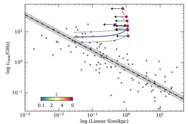
Figure 9: Spectral turnover as a function of linear size. The small gray circles are drawn from literature measurements of young radio AGN compiled by Jeyakumar (2016). The black dot-dashed line shows the empirical fit to the turnover-size relation from O’Dea (1998), and the dark gray shaded region indicates the uncertainty in the relation. Upper limits on the sizes of sources with quasi-simultaneous, multiband VLA follow-up from our sample that have spectroscopic redshifts available are shown by the large purple circles. For sources lacking redshifts, the linear size upper limits are shown over a range of possible redshifts as indicated by the rainbow-colored arcs.

5.6 Young Radio Jets

Young radio AGN, such as gigahertz-peaked spectrum (GPS) sources, are characterized by compact morphologies and inverted radio SEDs below their turnover (peak) frequencies, which are typically in the GHz regime (O’Dea, 1998), consistent with the morphologies and radio SEDs of the majority of our sources. After a jet is launched, models predict a rapid increase in luminosity ($P_{\rm radio}\sim t^{2/5}$) as the dominant energy-loss mechanism transitions from adiabatic to synchrotron losses (An & Baan, 2012), making the identification of young radio AGN in VLASS that have emerged in the time since the FIRST survey (17–24 yr for our sample) plausible. For a nascent radio jet that has been triggered within the past 20 yr, the model of An & Baan (2012) suggests an increase in radio luminosity of $>300$%. The identification of such young radio AGN is not unprecedented; the youngest known sources have kinematic ages as low as 20 yr (Gugliucci et al., 2005).

Based on the currently available radio continuum constraints, which include large variability amplitudes (with flux increases from 100% to $>$2500%) at 1.5 GHz compared to FIRST over timescales of decades, steady flux densities on timescales less than a few months at 3 GHz compared to VLASS, source size constraints $<0.1^{\prime\prime}$ ($\lesssim 1$ kpc), and curved radio SEDs peaking at $\sim$5–10 GHz, we find the radio properties of our sources to be consistent with young and compact radio AGN.

If the jet youth scenario for our sources is supported by higher-cadence, multiband follow-up data, there are exciting prospects for forthcoming radio surveys. Wide-area, broadband, synoptic radio surveys above a few GHz conducted over timescales of years to decades would be particularly well tuned for identifying large statistical samples of AGN with recently launched jets.

In Figure 9, we plot our sources on the turnover-size relation, along with a sample of young radio AGN from the literature. This relationship is believed to arise from the evolving radio spectral shapes of expanding young radio sources. As a young and compact radio source expands, the opacity due to SSA or FFA decreases, which causes the spectral peak (or turnover) to shift to lower frequencies (e.g. Bicknell et al. 1997; O’Dea 1998; Tingay & de Kool 2003). Since we only have upper limits on the linear sizes of our sources, we cannot yet directly confirm whether they follow the turnover-size relation. However, if we assume that our sources do follow the relation, we can obtain a rough estimate of their sizes.

As an example, we consider J0807+2102 at $z=1.5588$. The observed spectral turnover of this source is 21.9 GHz, which corresponds to a rest-frame turnover frequency of 56.2 GHz. Based on Figure 9, this implies a source size of 1–10 pc. Assuming a conservative value for the jet advance speed of $0.1c$, we obtain a rough estimate of the source age of $\sim$30–300 yr. Thus, the young jet model passes this important consistency check.

Very long baseline interferometric (VLBI) studies with sub-milliarcsecond resolution will ultimately be needed to test whether our sources are indeed compact on parsec scales, as expected for young jets. Nevertheless, the radio SED shapes and source size limits from the VLA data presented in this study are consistent with radio variability arising from the evolving radio SEDs of jets that have recently been triggered.

6 Discussion

Based on the radio properties of our sources, in particular their high luminosities, size constraints, variability amplitudes/timescales, and sky coordinates, we rule out extrinsic variability related to plasma propagation as a radio variability scenario. We also conclude that intrinsic variability associated with supernovae, GRBs, or TDEs is unlikely. We therefore favor an intrinsic AGN variability scenario in which the observed radio brightening is driven by a change in the SMBH accretion rate, jet reorientation, or the formation of newborn jets.

We emphasize that multiple mechanisms may contribute to the observed radio variability in a given source. A source could simultaneously be young, mildly Doppler boosted, and flaring owing to the propagation of shocks along the jet. Since our source flux densities are typically steady on timescales of a few months but vary substantially (100% to $>$2500%) over timescales of two decades, we find jet youth and/or jet reorientation to be the most plausible radio variability scenarios.

6.1 Accretion State Change

The large observed changes in radio flux may be associated with AGN transitioning between a radio-quiet state to one in which synchrotron-emitting radio jets are present. Extreme radio variability is typical of Galactic radio sources such as X-ray binaries (e.g. Mirabel & Rodríguez, 1999). In these sources, the short timescales associated with black holes with masses $\sim 1-10\,M_{\odot}$ mean that the change in state from a radio-quiet mode associated with soft X-ray emission to a mode with a hard X-ray spectrum and radio jets can happen on timescales of minutes. Given the $\sim 10^{7}-10^{9}\,M_{\odot}$ SMBH masses that are typical of AGN, similar transitions may occur (Maccarone et al., 2003; Falcke et al., 2004; Nipoti et al., 2005; Körding et al., 2006), but the corresponding timescales may be longer.

Previous attempts have been made to identify radio sources whose jets may have recently switched off (e.g. Marecki & Swoboda, 2011), but such objects still have radio emission from their lobes (though such sources are interesting in their own right in the context of restarted jets). An alternative approach is to identify AGN with a new onset of radio activity potentially associated with jets that have recently switched on. By their very nature these objects are expected to be relatively rare, but by surveying the radio emission from a large number of AGN in two or more well-separated epochs, it may be possible to find objects that are candidates for AGN undergoing this transition.

6.2 Comparison to Previous Studies

Although rare, previous studies have identified quasars with high-amplitude radio variability over timescales of years to decades (de Vries et al., 2004; Barvainis et al., 2005; Prandoni et al., 2010; Bell et al., 2015). In the Caltech NRAO Stripe 82 Survey (CNSS) pilot survey, Mooley et al. (2016) reported the detection of a single radio-loud type 2 quasar at $z=1.65$ (VTC233002-002736) that lacked any detectable emission in the FIRST survey. Follow-up observations revealed a nearly ten-fold flux increase at 1.5 GHz over a 15 year period and a curved radio SED, very similar in nature to our sources. Another example of such behavior in the CNSS, found in the $z=0.94$ quasar CNSS 013815+00, has been reported recently by Kunert-Bajraszewska et al. (2020). A newborn expanding radio jet is responsible for GPS-like characteristics of the radio spectrum of 013815+00. In addition, the transition from the radio-quiet to the radio-loud phase in 013815+00 coincides with changes in its accretion disk luminosity. Thus, the burst of radio activity in 013815+00 is interpreted as a result of an enhancement in the SMBH accretion rate. We note that only 013815+00 is identified in the Pâris et al. (2018) SDSS quasar catalog, but both of the CNSS quasars are classified as AGN in the mid-infrared by Assef et al. (2018) and would therefore meet the AGN and radio selection criteria of our sample (see Section 2).

We note that only one source matching our selection criteria was identified in the 50 deg² pilot CNSS footprint. This is loosely consistent (within a factor of a few) with our observed detection rate so far over 3440 deg² of the VLASS-FIRST footprint of one confirmed optical or infrared AGN with newly radio-loud activity per $\sim 20\pm 13$ deg². A more formal assessment of the areal density of AGN that have transitioned from radio-quiet to radio-loud on decades-long timescales that incorporates the entirety of VLASS Epoch 1 will be presented in a future study.

6.3 Implications for Galaxy Evolution

The large-scale radio jets and lobes launched by some active galactic nuclei (AGN) are believed to have long lifetimes and duty cycles on the order of millions of years. The properties of such “classical” radio AGN contrast sharply with those of radio jets featuring compact (subgalactic) extents, younger ages (decades to thousands of years), and shorter lifetimes that have previously been identified (Lähteenmäki et al., 2018; Kunert-Bajraszewska et al., 2020).

In the case of re-orienting jets, the change in jet direction may facilitate the transfer of energy over a large volume of the ISM of the host galaxy, thus potentially influencing ambient ISM conditions (Gaibler et al., 2011; Mukherjee et al., 2016). However, the prevalence and basic physical properties of re-orienting jets, regardless of origin (see Section 5.5), have not been well constrained owing to inherent observational challenges (the combined requirements of high angular resolution imaging and high-cadence monitoring). If re-orienting compact jets are common, particularly at $z>1$, they may contribute substantially to SMBH-galaxy co-evolution via the regulation of star formation from jet-ISM feedback or a disruption in SMBH growth in response to the launching of a jet.

Intermittent, albeit short-lived, episodes of radio-loud activity associated with powerful AGN may also be important in the context of galaxy evolution. Numerous studies over the past few decades have used a variety of arguments (such as the overrepresentation of compact jetted AGN in flux-limited surveys) in favor of the existence of a large population of short-lived and/or rapidly retriggered compact radio AGN (Czerny et al. 2009; Mooley et al. 2016; Jarvis et al. 2019; Patil et al. 2020; Shabala et al. 2020). As a rough assessment of whether the rate of newly radio-loud AGN identified in VLASS so far is consistent with this possibility, we compare the areal densities of the overall radio-loud AGN population based on constraints from FIRST with our sample. Ivezić et al. (2002) found 1154 SDSS quasars detected by FIRST over 774 deg², corresponding to an areal density of radio-loud quasars of $\sim$1 deg^-2. If these quasars have a lifetime of $\sim$10⁶ yr, we would only expect a very small fraction, $\sim$1 in 10⁵, to be within their first decade of being identified as radio-loud. This translates to an areal density of $\sim$10^-5 deg^-2 compared to our detection rate of 13 newly radio-loud type 1 quasars in 3,440 deg², i.e. $\sim 4\times 10^{-3}$ deg^-2, consistent with a typical period of occurrence of $\sim$10⁵ yr.

We speculate that frequent episodes of short-lived AGN jets that do not necessarily grow to large scales could be associated with higher-efficiency jet-driven feedback into the hosts of high-$z$ galaxies. A similar conclusion was reached by van Velzen et al. (2015), who found that the fraction of powerful jets that grow beyond $\sim 100$ kpc scales decreases with redshift. Future studies investigating the ISM content and conditions of the hosts of newly radio-loud AGN will be important for placing quantitative constraints on the energetic impact of feedback from compact jets at cosmic noon.

7 Summary

As part of an ongoing search for slow radio transients between FIRST and VLASS Epoch 1 covering 3,440 deg² so far, we have identified a sample of 26 sources with radio variability on decadal timescales associated with known powerful quasars in SDSS and/or WISE. These sources were previously radio-quiet quasars in FIRST but are now consistent with the radio-loud quasar population following their detection in VLASS Epoch 1.

To investigate the origin of the radio variability in our sample of newly radio-loud quasars, we performed multiband, quasi-simultaneous VLA follow-up observations of 14 sources. All of our sources are characterized by high radio luminosities ($L_{\rm 3\,GHz}=10^{40-42}\,\,{\rm erg}\,{\rm s}^{-1}$) in the quasar regime, compact ($\lesssim 0.1^{\prime\prime}$) emission, and broadband radio SEDs from 1–18 GHz with significant spectral curvature.

A comparison between the VLASS images (all of which were observed in 2019 during Epoch 1.2) and our follow-up VLA $S$-band data a few months later revealed good agreement within the current $\sim$20% flux uncertainties of VLASS, suggesting a typical variability timescale longer than a few months. At $L$-band, the observed variability amplitudes range from 100% to $>$2500% in the 17–24 yr since FIRST.

Based on the radio properties of our sources, including their SED shapes, variability timescale and amplitude constraints, and high radio luminosities, we conclude that variability due to extrinsic propagation effects or transient phenomena (including GRBs, supernovae, and TDEs) is unlikely. We therefore favor an intrinsic AGN variability scenario for our sample.

We conclude that our sources are most consistent with powerful quasars hosting compact, possibly young jets, which poses a challenge the generally accepted idea that “radio-loudness” is a property of the quasar/AGN population that remains fixed on human timescales. Our study suggests that frequent episodes of short-lived AGN jets that do not necessarily grow to large scales may be common at high redshift. We speculate that intermittent but powerful jets on subgalactic scales could interact with the interstellar medium leading to feedback that could influence the evolution of galaxies at cosmic noon.

Further multiband follow-up with the VLA, as well as parsec-scale imaging with the Very Long Baseline Array, will be essential for placing tighter constraints on the evolutionary stages of our sources. Additional follow-up efforts across the electromagnetic spectrum, including optical/infrared observations to determine the basic properties of the host galaxies, studies of the molecular gas content and conditions using millimeter/submillimeter telescopes, and explorations of the accretion physics and large-scale environments from high-energy (e.g. X-ray) data, will be required.

Ultimately, the completion of the remaining two VLASS epochs, as well as future surveys of the dynamic radio and millimeter sky with the Square Kilometre Array and its pathfinders (e.g., Bignall et al. 2015; Murphy et al. 2013), will provide new insights into the life cycles of radio jets. In addition to radio surveys, detailed studies of individual objects quantifying the impact of jets on their ambient environments with telescopes such as the Atacama Large Millimeter/Submillimeter Array and the next-generation Very Large Array (Nyland et al., 2018) will be essential for determining the overall importance of feedback on ISM scales driven by compact jets for galaxy evolution.

Appendix A Source Properties

The basic properties of our sources from our multiband VLA follow-up observations are presented in Table 6. We note that all sources are unresolved at the angular resolution provided in Column 6 of Table 6.

Table 6: Multiband VLA Follow-up Data

Source	Date	Band	$\nu$	$\sigma_{\rm rms}$	$\theta_{\rm maj}\times\theta_{\rm min}$	$S_{\rm peak}$
			(GHz)	($\mu$mJy beam-1)	($\prime\prime\times\prime\prime$)	(mJy beam-1)
(1)	(2)	(3)	(4)	(5)	(6)	(7)
J0742+2704	2019 Oct 03	L	1.5	47	$2.00\times 0.89$	$3.80\pm 0.04$
		S	3.0	25	$0.95\times 0.49$	$10.97\pm 0.02$
		C	6.0	20	$0.43\times 0.25$	$25.20\pm 0.04$
		X	10.0	20	$0.27\times 0.18$	$25.23\pm 0.03$
		Ku	15.0	10	$0.17\times 0.12$	$19.70\pm 0.01$
J0807+2102	2019 July 23	L	1.5	187	$4.44\times 1.11$	$0.86\pm 0.03$
		S	3.0	87	$2.31\times 0.57$	$3.15\pm 0.07$
		C	6.0	45	$1.15\times 0.28$	$7.83\pm 0.03$
		X	10.0	26	$0.67\times 0.20$	$15.10\pm 0.02$
	2019 Sept 19	X	10.0	15	$0.28\times 0.19$	$16.83\pm 0.02$
		Ku	15.0	13	$0.18\times 0.13$	$17.42\pm 0.01$
		K	22.0	28	$0.11\times 0.09$	$13.03\pm 0.03$
J0832+2302	2019 July 23	L	1.5	70	$4.63\times 1.11$	$1.41\pm 0.05$
		S	3.0	35	$2.33\times 0.65$	$3.25\pm 0.03$
		C	6.0	20	$1.14\times 0.34$	$5.69\pm 0.01$
		X	10.0	21	$0.71\times 0.21$	$5.28\pm 0.02$
	2019 Sept 19	X	10.0	13	$0.26\times 0.19$	$5.97\pm 0.01$
		Ku	15.0	21	$0.17\times 0.12$	$6.57\pm 0.02$
J0950+5128	2019 July 23	L	1.5	58	$4.11\times 1.48$	$3.93\pm 0.05$
		S	3.0	41	$2.23\times 0.68$	$10.21\pm 0.02$
		C	6.0	19	$1.10\times 0.39$	$15.61\pm 0.02$
		X	10.0	23	$0.65\times 0.24$	$17.09\pm 0.02$
	2019 Sept 19	X	10.0	12	$0.28\times 0.19$	$18.69\pm 0.01$
		Ku	15.0	33	$0.16\times 0.13$	$13.12\pm 0.05$
J1037-0736	2019 Oct 13	L	1.5	69	$1.79\times 1.10$	$6.68\pm 0.07$
		S	3.0	68	$0.72\times 0.53$	$15.48\pm 0.07$
		C	6.0	22	$0.34\times 0.26$	$19.13\pm 0.06$
		X	10.0	16	$0.24\times 0.16$	$16.08\pm 0.02$
		Ku	15.0	14	$0.17\times 0.11$	$13.31\pm 0.01$
J1204+1918	2019 Oct 11	L	1.5	90	$1.32\times 1.14$	$2.00\pm 0.01$
		S	3.0	26	$0.70\times 0.55$	$4.83\pm 0.02$
		C	6.0	15	$0.32\times 0.31$	$5.10\pm 0.01$
		X	10.0	18	$0.23\times 0.18$	$3.20\pm 0.01$
		Ku	15.0	13	$0.16\times 0.12$	$2.00\pm 0.01$
J1208+4741	2019 Oct 11	L	1.5	41	$1.14\times 0.98$	$1.06\pm 0.01$
		S	3.0	18	$0.62\times 0.49$	$2.46\pm 0.01$
		C	6.0	13	$0.29\times 0.25$	$2.95\pm 0.01$
		X	10.0	15	$0.18\times 0.15$	$2.29\pm 0.01$
		Ku	15.0	13	$0.12\times 0.10$	$1.74\pm 0.01$
J1246+1805	2019 Oct 11	L	1.5	130	$1.45\times 1.17$	$3.39\pm 0.01$
		S	3.0	43	$0.76\times 0.56$	$8.25\pm 0.02$
		C	6.0	23	$0.32\times 0.27$	$11.58\pm 0.02$
		X	10.0	28	$0.18\times 0.18$	$12.20\pm 0.01$
		Ku	15.0	25	$0.13\times 0.11$	$11.75\pm 0.03$
J1254-0606	2019 Nov 01	L	1.5	80	$1.70\times 0.89$	$1.69\pm 0.08$
		S	3.0	74	$0.90\times 0.55$	$10.06\pm 0.03$
		C	6.0	37	$0.33\times 0.23$	$18.51\pm 0.05$
		X	10.0	28	$0.22\times 0.15$	$15.03\pm 0.05$
		Ku	15.0	26	$0.15\times 0.10$	$9.39\pm 0.04$
J1413+0257	2019 Sept 23	L	1.5	63	$1.45\times 1.04$	$1.38\pm 0.06$
		S	3.0	23	$0.87\times 0.60$	$7.30\pm 0.02$
		C	6.0	22	$0.40\times 0.25$	$14.58\pm 0.02$
		X	10.0	15	$0.30\times 0.19$	$10.92\pm 0.01$
		Ku	15.0	12	$0.21\times 0.12$	$6.68\pm 0.01$
J1447+0512	2019 Sept 23	L	1.5	48	$1.55\times 1.09$	$2.71\pm 0.05$
		S	3.0	21	$0.92\times 0.58$	$4.02\pm 0.02$
		C	6.0	12	$0.49\times 0.30$	$2.38\pm 0.01$
		X	10.0	15	$0.32\times 0.19$	$1.55\pm 0.01$
		Ku	15.0	11	$0.18\times 0.13$	$1.30\pm 0.01$
J1546+1500	2019 Sept 23	L	1.5	39	$1.41\times 1.15$	$3.30\pm 0.04$
		S	3.0	21	$0.76\times 0.58$	$5.61\pm 0.02$
		C	6.0	12	$0.42\times 0.30$	$5.28\pm 0.01$
		X	10.0	14	$0.26\times 0.19$	$4.03\pm 0.01$
		Ku	15.0	21	$0.16\times 0.10$	$3.50\pm 0.02$
J1603+1809	2019 Sept 23	L	1.5	40	$1.22\times 1.01$	$0.88\pm 0.04$
		S	3.0	18	$0.71\times 0.58$	$3.16\pm 0.01$
		C	6.0	12	$0.38\times 0.30$	$5.85\pm 0.01$
		X	10.0	15	$0.24\times 0.19$	$5.81\pm 0.01$
		Ku	15.0	12	$0.17\times 0.12$	$4.80\pm 0.01$
J2109-0644	2019 Sept 10	L	1.5	58	$1.43\times 1.06$	$11.17\pm 0.05$
		S	3.0	22	$0.80\times 0.57$	$12.51\pm 0.01$
		C	6.0	15	$0.39\times 0.29$	$16.97\pm 0.01$
		X	10.0	10	$0.25\times 0.18$	$15.79\pm 0.01$
		Ku	15.0	11	$0.17\times 0.11$	$13.00\pm 0.02$

Note. — Column 1: Source name. Column 2: Observing date(s). Column 3: VLA band, defined as follows: L: 1–2 GHz, S: 2–4 GHz, C: 4–8 GHz, X: 8–12 GHz, Ku: 12–18 GHz, K: 18–26 GHz. Column 4: Central image frequency. Column 5: 1$\sigma$ rms noise. Column 6: Clean beam dimensions (major $\times$ minor axis). Column 7: Peak flux density.

References

- Alexander et al. (2020) Alexander, K. D., van Velzen, S., Horesh, A., & Zauderer, B. A. 2020, Space Sci. Rev., 216, 81
- An & Baan (2012) An, T., & Baan, W. A. 2012, ApJ, 760, 77
- An et al. (2013) An, T., Baan, W. A., Wang, J.-Y., Wang, Y., & Hong, X.-Y. 2013, MNRAS, 434, 3487
- An et al. (2020) An, T., Mohan, P., Zhang, Y., et al. 2020, Nature Communications, 11, 143
- Anderson et al. (2020) Anderson, M. M., Mooley, K. P., Hallinan, G., et al. 2020, ApJ, 903, 116
- Anjum et al. (2020) Anjum, A., Stalin, C. S., Rakshit, S., Gudennavar, S. B., & Durgapal, A. 2020, MNRAS, 494, 764
- Assef et al. (2018) Assef, R. J., Stern, D., Noirot, G., et al. 2018, ApJS, 234, 23
- Astropy Collaboration et al. (2013) Astropy Collaboration, Robitaille, T. P., Tollerud, E. J., et al. 2013, A&A, 558, A33
- Bannister et al. (2011) Bannister, K. W., Murphy, T., Gaensler, B. M., Hunstead, R. W., & Chatterjee, S. 2011, Monthly Notices of the Royal Astronomical Society, 412, 634. https://doi.org/10.1111/j.1365-2966.2010.17938.x
- Bannister et al. (2016) Bannister, K. W., Stevens, J., Tuntsov, A. V., et al. 2016, Science, 351, 354
- Barvainis et al. (2005) Barvainis, R., Lehár, J., Birkinshaw, M., Falcke, H., & Blundell, K. M. 2005, ApJ, 618, 108
- Becker et al. (1995) Becker, R. H., White, R. L., & Helfand, D. J. 1995, ApJ, 450, 559
- Bell et al. (2015) Bell, M. E., Huynh, M. T., Hancock, P., et al. 2015, MNRAS, 450, 4221
- Berger (2014) Berger, E. 2014, ARA&A, 52, 43
- Berriman & Good (2017) Berriman, G. B., & Good, J. C. 2017, PASP, 129, 058006
- Bicknell et al. (1997) Bicknell, G. V., Dopita, M. A., & O’Dea, C. P. O. 1997, ApJ, 485, 112
- Bicknell et al. (2018) Bicknell, G. V., Mukherjee, D., Wagner, A. e. Y., Sutherland, R. S., & Nesvadba, N. P. H. 2018, MNRAS, 475, 3493
- Bignall et al. (2015) Bignall, H. E., Croft, S., Hovatta, T., et al. 2015, Advancing Astrophysics with the Square Kilometre Array (AASKA14), 58
- Blandford et al. (2019) Blandford, R., Meier, D., & Readhead, A. 2019, ARA&A, 57, 467
- Bonnerot et al. (2016) Bonnerot, C., Rossi, E. M., & Lodato, G. 2016, MNRAS, 458, 3324
- Böttcher (2019) Böttcher, M. 2019, Galaxies, 7, 20
- Braun et al. (2019) Braun, R., Bonaldi, A., Bourke, T., Keane, E., & Wagg, J. 2019, arXiv e-prints, arXiv:1912.12699
- Braun et al. (2015) Braun, R., Bourke, T., Green, J. A., Keane, E., & Wagg, J. 2015, in Advancing Astrophysics with the Square Kilometre Array (AASKA14), 174
- Briggs (1995) Briggs, D. S. 1995, in Bulletin of the American Astronomical Society, Vol. 27, American Astronomical Society Meeting Abstracts, 1444
- Britzen et al. (2017) Britzen, S., Qian, S. J., Steffen, W., et al. 2017, A&A, 602, A29
- Brunthaler et al. (2005) Brunthaler, A., Falcke, H., Bower, G. C., et al. 2005, A&A, 435, 497
- Burke-Spolaor et al. (2019) Burke-Spolaor, S., Taylor, S. R., Charisi, M., et al. 2019, A&A Rev., 27, 5
- Callingham et al. (2015) Callingham, J. R., Gaensler, B. M., Ekers, R. D., et al. 2015, ApJ, 809, 168
- Callingham et al. (2017) Callingham, J. R., Ekers, R. D., Gaensler, B. M., et al. 2017, ApJ, 836, 174
- Carilli et al. (2003) Carilli, C. L., Ivison, R. J., & Frail, D. A. 2003, ApJ, 590, 192
- Cendes (2020) Cendes, Y. 2020, PhD thesis, Leiden University
- Chandra & Frail (2012) Chandra, P., & Frail, D. A. 2012, ApJ, 746, 156
- Chatterjee et al. (2011) Chatterjee, R., Marscher, A. P., Jorstad, S. G., et al. 2011, ApJ, 734, 43
- Chhetri et al. (2018) Chhetri, R., Morgan, J., Ekers, R. D., et al. 2018, MNRAS, 474, 4937
- Clarke et al. (2016) Clarke, T. E., Kassim, N. E., Brisken, W., et al. 2016, in Society of Photo-Optical Instrumentation Engineers (SPIE) Conference Series, Vol. 9906, Ground-based and Airborne Telescopes VI, 99065B
- Clegg et al. (1998) Clegg, A. W., Fey, A. L., & Lazio, T. J. W. 1998, ApJ, 496, 253
- Collier et al. (2018) Collier, J. D., Tingay, S. J., Callingham, J. R., et al. 2018, MNRAS, 477, 578
- Cordes & Lazio (2002) Cordes, J. M., & Lazio, T. J. W. 2002, arXiv e-prints, astro
- Cordes & Lazio (2003) —. 2003, arXiv e-prints, astro
- Cornwell et al. (2005) Cornwell, T. J., Golap, K., & Bhatnagar, S. 2005, in Astronomical Society of the Pacific Conference Series, Vol. 347, Astronomical Data Analysis Software and Systems XIV, ed. P. Shopbell, M. Britton, & R. Ebert, 86
- Cotton (2008) Cotton, W. D. 2008, PASP, 120, 439
- Cutri & et al. (2013) Cutri, R. M., & et al. 2013, VizieR Online Data Catalog, II/328
- Czerny et al. (2009) Czerny, B., Siemiginowska, A., Janiuk, A., Nikiel-Wroczyński, B., & Stawarz, Ł. 2009, ApJ, 698, 840
- Dai et al. (2020) Dai, B. B., Shu, X. W., Jiang, N., et al. 2020, ApJ, 896, L27
- de Vries et al. (2004) de Vries, W. H., Becker, R. H., White, R. L., & Helfand , D. J. 2004, AJ, 127, 2565
- Dewdney et al. (2009) Dewdney, P. E., Hall, P. J., Schilizzi, R. T., & Lazio, T. J. L. W. 2009, Proceedings of the IEEE, 97, 1482
- Duffy & Blundell (2012) Duffy, P., & Blundell, K. M. 2012, MNRAS, 421, 108
- Eftekhari et al. (2018) Eftekhari, T., Berger, E., Zauderer, B. A., Margutti, R., & Alexander, K. D. 2018, ApJ, 854, 86
- Falcke et al. (2004) Falcke, H., Körding, E., & Markoff, S. 2004, A&A, 414, 895
- Fanaroff & Riley (1974) Fanaroff, B. L., & Riley, J. M. 1974, MNRAS, 167, 31P
- Fawcett et al. (2020) Fawcett, V. A., Alexander, D. M., Rosario, D. J., et al. 2020, MNRAS, 494, 4802
- Fiedler et al. (1987) Fiedler, R. L., Dennison, B., Johnston, K. J., & Hewish, A. 1987, Nature, 326, 675
- Fossati et al. (1998) Fossati, G., Maraschi, L., Celotti, A., Comastri, A., & Ghisellini, G. 1998, MNRAS, 299, 433
- Frail et al. (2012) Frail, D. A., Kulkarni, S. R., Ofek, E. O., Bower, G. C., & Nakar, E. 2012, ApJ, 747, 70
- Fromm et al. (2015) Fromm, C. M., Fuhrmann, L., & Perucho, M. 2015, A&A, 580, A94
- Gaibler et al. (2011) Gaibler, V., Khochfar, S., & Krause, M. 2011, MNRAS, 411, 155
- Georgakakis et al. (2012) Georgakakis, A., Grossi, M., Afonso, J., & Hopkins, A. M. 2012, MNRAS, 421, 2223
- Glikman et al. (2012) Glikman, E., Urrutia, T., Lacy, M., et al. 2012, ApJ, 757, 51
- Graham et al. (2019) Graham, M. J., Kulkarni, S. R., Bellm, E. C., et al. 2019, PASP, 131, 078001
- Gralla et al. (2020) Gralla, M. B., Marriage, T. A., Addison, G., et al. 2020, ApJ, 893, 104
- Gugliucci et al. (2005) Gugliucci, N. E., Taylor, G. B., Peck, A. B., & Giroletti, M. 2005, ApJ, 622, 136
- Heckman & Best (2014) Heckman, T. M., & Best, P. N. 2014, ARA&A, 52, 589
- Helfand et al. (2015) Helfand, D. J., White, R. L., & Becker, R. H. 2015, ApJ, 801, 26
- Hills (1975) Hills, J. G. 1975, Nature, 254, 295
- Holgado et al. (2018) Holgado, A. M., Sesana, A., Sandrinelli, A., et al. 2018, MNRAS, 481, L74
- Hovatta et al. (2007) Hovatta, T., Tornikoski, M., Lainela, M., et al. 2007, A&A, 469, 899
- Husemann et al. (2019) Husemann, B., Bennert, V. N., Jahnke, K., et al. 2019, ApJ, 879, 75
- Ivezić et al. (2002) Ivezić, Ž., Menou, K., Knapp, G. R., et al. 2002, AJ, 124, 2364
- Jacob et al. (2010) Jacob, J. C., Katz, D. S., Berriman, G. B., et al. 2010, arXiv e-prints, arXiv:1005.4454
- Janiuk & Czerny (2011) Janiuk, A., & Czerny, B. 2011, MNRAS, 414, 2186
- Jarvis et al. (2019) Jarvis, M. E., Harrison, C. M., Thomson, A. P., et al. 2019, MNRAS, 485, 2710
- Jauncey et al. (2016) Jauncey, D., Bignall, H., Kedziora-Chudczer, L., et al. 2016, Galaxies, 4, 62
- Jeyakumar (2016) Jeyakumar, S. 2016, MNRAS, 458, 3786
- Kaplan et al. (2011) Kaplan, D. L., O’Shaughnessy, R., Sesana, A., & Volonteri, M. 2011, ApJ, 734, L37
- Keim et al. (2019) Keim, M. A., Callingham, J. R., & Röttgering, H. J. A. 2019, A&A, 628, A56
- Kellermann et al. (2016) Kellermann, K. I., Condon, J. J., Kimball, A. E., Perley, R. A., & Ivezić, Ž. 2016, ApJ, 831, 168
- Kesden (2012) Kesden, M. 2012, Phys. Rev. D, 85, 024037
- Khan et al. (2018) Khan, A., Paschalidis, V., Ruiz, M., & Shapiro, S. L. 2018, Phys. Rev. D, 97, 044036
- Klindt et al. (2019) Klindt, L., Alexander, D. M., Rosario, D. J., Lusso, E., & Fotopoulou, S. 2019, MNRAS, 488, 3109
- Koay et al. (2016) Koay, J. Y., Vestergaard, M., Bignall, H. E., Reynolds, C., & Peterson, B. M. 2016, MNRAS, 460, 304
- Komossa (2015) Komossa, S. 2015, Journal of High Energy Astrophysics, 7, 148
- Komossa et al. (2020) Komossa, S., Grupe, D., Parker, M. L., et al. 2020, MNRAS, 498, L35
- Körding et al. (2006) Körding, E. G., Jester, S., & Fender, R. 2006, MNRAS, 372, 1366
- Kulkarni & Loeb (2016) Kulkarni, G., & Loeb, A. 2016, MNRAS, 456, 3964
- Kunert-Bajraszewska et al. (2010) Kunert-Bajraszewska, M., Janiuk, A., Gawroński, M. P., & Siemiginowska, A. 2010, ApJ, 718, 1345
- Kunert-Bajraszewska et al. (2020) Kunert-Bajraszewska, M., Wołowska, A., Mooley, K., Kharb, P., & Hallinan, G. 2020, ApJ, 897, 128
- Lacy et al. (2020) Lacy, M., Baum, S. A., Chandler, C. J., et al. 2020, PASP, 132, 035001
- Lähteenmäki et al. (2018) Lähteenmäki, A., Järvelä, E., Ramakrishnan, V., et al. 2018, A&A, 614, L1
- Law et al. (2018) Law, C. J., Gaensler, B. M., Metzger, B. D., Ofek, E. O., & Sironi, L. 2018, ApJ, 866, L22
- Lister (2001) Lister, M. L. 2001, ApJ, 561, 676
- Lister et al. (2020) Lister, M. L., Homan, D. C., Kovalev, Y. Y., et al. 2020, ApJ, 899, 141
- Lonsdale et al. (2015) Lonsdale, C. J., Lacy, M., Kimball, A. E., et al. 2015, ApJ, 813, 45
- Maccagni et al. (2020) Maccagni, F. M., Murgia, M., Serra, P., et al. 2020, A&A, 634, A9
- Maccarone et al. (2003) Maccarone, T. J., Gallo, E., & Fender, R. 2003, MNRAS, 345, L19
- MacLeod et al. (2012) MacLeod, M., Guillochon, J., & Ramirez-Ruiz, E. 2012, ApJ, 757, 134
- Mainzer et al. (2011) Mainzer, A., Bauer, J., Grav, T., et al. 2011, ApJ, 731, 53
- Marecki & Swoboda (2011) Marecki, A., & Swoboda, B. 2011, A&A, 525, A6
- Marscher & Gear (1985) Marscher, A. P., & Gear, W. K. 1985, ApJ, 298, 114
- Mateos et al. (2012) Mateos, S., Alonso-Herrero, A., Carrera, F. J., et al. 2012, MNRAS, 426, 3271
- McMullin et al. (2007) McMullin, J. P., Waters, B., Schiebel, D., Young, W., & Golap, K. 2007, in Astronomical Society of the Pacific Conference Series, Vol. 376, Astronomical Data Analysis Software and Systems XVI, ed. R. A. Shaw, F. Hill, & D. J. Bell, 127
- Meyer et al. (2011) Meyer, E. T., Fossati, G., Georganopoulos, M., & Lister, M. L. 2011, ApJ, 740, 98
- Mhaskey et al. (2019a) Mhaskey, M., Gopal-Krishna, Dabhade, P., et al. 2019a, MNRAS, 485, 2447
- Mhaskey et al. (2019b) Mhaskey, M., Gopal-Krishna, Paul, S., et al. 2019b, MNRAS, 489, 3506
- Middelberg et al. (2007) Middelberg, E., Agudo, I., Roy, A. L., & Krichbaum, T. P. 2007, MNRAS, 377, 731
- Mirabel & Rodríguez (1999) Mirabel, I. F., & Rodríguez, L. F. 1999, ARA&A, 37, 409
- Mooley et al. (2016) Mooley, K. P., Hallinan, G., Bourke, S., et al. 2016, ApJ, 818, 105
- Morgan et al. (2018) Morgan, J. S., Macquart, J. P., Ekers, R., et al. 2018, MNRAS, 473, 2965
- Morganti et al. (2013) Morganti, R., Fogasy, J., Paragi, Z., Oosterloo, T., & Orienti, M. 2013, Science, 341, 1082
- Mukherjee et al. (2016) Mukherjee, D., Bicknell, G. V., Sutherland , R., & Wagner, A. 2016, MNRAS, 461, 967
- Mukherjee et al. (2018) Mukherjee, D., Wagner, A. Y., Bicknell, G. V., et al. 2018, MNRAS, 476, 80
- Mundell et al. (2009) Mundell, C. G., Ferruit, P., Nagar, N., & Wilson, A. S. 2009, ApJ, 703, 802
- Murphy et al. (2018) Murphy, E. J., Bolatto, A., Chatterjee, S., et al. 2018, in Astronomical Society of the Pacific Conference Series, Vol. 517, Science with a Next Generation Very Large Array, ed. E. Murphy, 3
- Murphy et al. (2013) Murphy, T., Chatterjee, S., Kaplan, D. L., et al. 2013, PASA, 30, e006
- Narayan (1992) Narayan, R. 1992, Philosophical Transactions of the Royal Society of London Series A, 341, 151
- Nipoti et al. (2005) Nipoti, C., Blundell, K. M., & Binney, J. 2005, MNRAS, 361, 633
- Nyland et al. (2013) Nyland, K., Alatalo, K., Wrobel, J. M., et al. 2013, ApJ, 779, 173
- Nyland et al. (2018) Nyland, K., Harwood, J. J., Mukherjee, D., et al. 2018, ApJ, 859, 23
- O’Dea (1998) O’Dea, C. P. 1998, PASP, 110, 493
- O’Dea & Saikia (2020) O’Dea, C. P., & Saikia, D. J. 2020, arXiv e-prints, arXiv:2009.02750
- Orienti (2016) Orienti, M. 2016, Astronomische Nachrichten, 337, 9
- Orienti & Dallacasa (2020) Orienti, M., & Dallacasa, D. 2020, MNRAS, 499, 1340
- Orienti et al. (2010) Orienti, M., Dallacasa, D., & Stanghellini, C. 2010, MNRAS, 408, 1075
- Padmanabhan & Loeb (2020) Padmanabhan, H., & Loeb, A. 2020, arXiv e-prints, arXiv:2003.07365
- Palenzuela et al. (2010) Palenzuela, C., Lehner, L., & Liebling, S. L. 2010, Science, 329, 927
- Palliyaguru et al. (2019) Palliyaguru, N. T., Corsi, A., Frail, D. A., et al. 2019, ApJ, 872, 201
- Pâris et al. (2018) Pâris, I., Petitjean, P., Aubourg, É., et al. 2018, A&A, 613, A51
- Patil et al. (2020) Patil, P., Nyland, K., Whittle, M., et al. 2020, ApJ, 896, 18
- Perley & Butler (2013) Perley, R. A., & Butler, B. J. 2013, ApJS, 204, 19
- Perley & Butler (2017) —. 2017, ApJS, 230, 7
- Pietka et al. (2015) Pietka, M., Fender, R. P., & Keane, E. F. 2015, MNRAS, 446, 3687
- Planck Collaboration et al. (2016) Planck Collaboration, Ade, P. A. R., Aghanim, N., et al. 2016, A&A, 594, A13
- Polisensky et al. (2016) Polisensky, E., Lane, W. M., Hyman, S. D., et al. 2016, ApJ, 832, 60
- Prandoni et al. (2010) Prandoni, I., de Ruiter, H. R., Ricci, R., et al. 2010, A&A, 510, A42
- Rau & Cornwell (2011) Rau, U., & Cornwell, T. J. 2011, A&A, 532, A71
- Reynolds & Begelman (1997) Reynolds, C. S., & Begelman, M. C. 1997, ApJ, 487, L135
- Rosario et al. (2020) Rosario, D. J., Fawcett, V. A., Klindt, L., et al. 2020, MNRAS, 494, 3061
- Ruffa et al. (2019) Ruffa, I., Prandoni, I., Laing, R. A., et al. 2019, MNRAS, 484, 4239
- Sarbadhicary et al. (2020) Sarbadhicary, S. K., Tremou, E., Stewart, A. J., et al. 2020, arXiv e-prints, arXiv:2009.05056
- Schnittman (2013) Schnittman, J. D. 2013, Classical and Quantum Gravity, 30, 244007
- Selina et al. (2018) Selina, R. J., Murphy, E. J., McKinnon, M., et al. 2018, in Astronomical Society of the Pacific Conference Series, Vol. 517, Science with a Next Generation Very Large Array, ed. E. Murphy, 15
- Shabala et al. (2020) Shabala, S. S., Jurlin, N., Morganti, R., et al. 2020, MNRAS, 496, 1706
- Shen et al. (2011) Shen, Y., Richards, G. T., Strauss, M. A., et al. 2011, ApJS, 194, 45
- Siemiginowska et al. (2016) Siemiginowska, A., Sobolewska, M., Migliori, G., et al. 2016, ApJ, 823, 57
- Stanimirović & Zweibel (2018) Stanimirović, S., & Zweibel, E. G. 2018, ARA&A, 56, 489
- Thyagarajan et al. (2011) Thyagarajan, N., Helfand, D. J., White, R. L., & Becker, R. H. 2011, ApJ, 742, 49
- Tingay & de Kool (2003) Tingay, S. J., & de Kool, M. 2003, AJ, 126, 723
- Tingay et al. (2015) Tingay, S. J., Macquart, J. P., Collier, J. D., et al. 2015, AJ, 149, 74
- Tinti et al. (2005) Tinti, S., Dallacasa, D., de Zotti, G., Celotti, A., & Stanghellini, C. 2005, A&A, 432, 31
- Torniainen et al. (2005) Torniainen, I., Tornikoski, M., Teräsranta, H., Aller, M. F., & Aller, H. D. 2005, A&A, 435, 839
- van Velzen et al. (2018) van Velzen, S., Bower, G. C., & Metzger, B. D. 2018, in Astronomical Society of the Pacific Conference Series, Vol. 517, Science with a Next Generation Very Large Array, ed. E. Murphy, 737
- van Velzen et al. (2015) van Velzen, S., Falcke, H., & Körding, E. 2015, MNRAS, 446, 2985
- van Velzen et al. (2011) van Velzen, S., Körding, E., & Falcke, H. 2011, MNRAS, 417, L51
- van Velzen et al. (2016) van Velzen, S., Anderson, G. E., Stone, N. C., et al. 2016, Science, 351, 62
- Walker (1998) Walker, M. A. 1998, MNRAS, 294, 307
- Weiler et al. (2002) Weiler, K. W., Panagia, N., Montes, M. J., & Sramek, R. A. 2002, ARA&A, 40, 387
- Williams et al. (2020) Williams, D. R. A., Baldi, R. D., McHardy, I. M., et al. 2020, MNRAS, 495, 3079
- Wołowska et al. (2017) Wołowska, A., Kunert-Bajraszewska, M., Mooley, K., & Hallinan, G. 2017, Frontiers in Astronomy and Space Sciences, 4, 38
- Woosley & Bloom (2006) Woosley, S. E., & Bloom, J. S. 2006, ARA&A, 44, 507
- Wright et al. (2010) Wright, E. L., Eisenhardt, P. R. M., Mainzer, A. K., et al. 2010, AJ, 140, 1868
- York et al. (2000) York, D. G., Adelman, J., Anderson, Jr., J. E., et al. 2000, AJ, 120, 1579