Runaway blue main-sequence stars at high Galactic latitudes

Abstract

Context. The ESA Gaia mission is a remarkable tool for stellar population analysis through its accurate Hertzsprung-Russell diagram. Its precise astrometry has propelled detailed kinematic studies of the Milky Way and the identification of high-velocity outliers.

Aims. Motivated by the historical identification of runaway main-sequence (MS) stars of early spectral type at high Galactic latitudes, we test the capability of Gaia at identifying new such stars.

Methods. We have selected $\approx 2300$ sources with Gaia magnitudes of $G_{\rm BP}-G_{\rm RP}\leq 0.05$, compatible with the colors of low-extinction MS stars earlier than mid-A spectral type, and obtained low-resolution optical spectroscopy for 48 such stars. By performing detailed photometric and spectroscopic analyses, we derive their atmospheric and physical parameters (effective temperature, surface gravity, radial velocity, interstellar reddening, spectrophotometric distance, mass, radius, luminosity, and age). The comparison between spectrophotometric and parallax-based distances enables us to disentangle the MS candidates from older blue horizontal branch (BHB) candidates.

Results. We identify 12 runaway MS candidates, with masses between 2 and 6 M_☉. Their trajectories are traced back to the Galactic disc to identify their most recent Galactic plane crossings and the corresponding flight times. All 12 candidates are ejected from the Galactic disc within 2 to 16.5 kpc from the Galactic center and possess flight times that are shorter than their evolutionary ages, compatible with a runaway hypothesis. Three MS candidates have ejection velocities exceeding 450 km s^-1, thus, appear to challenge the canonical ejection scenarios for late B-type stars. The fastest star of our sample also has a non-negligible Galactic escape probability if its MS nature can be confirmed. We identify 27 BHB candidates, and the two hottest stars in our sample are rare late O and early B type stars of low mass evolving towards the white dwarf cooling sequence.

Conclusions. The combination of Gaia parallaxes and proper motions can lead to the efficient selection of runaway blue MS candidates up to 10 kpc away from the Sun. High resolution spectra are needed to confirm the MS status, via precise measurements of projected rotational velocities and chemical compositions.

1 Introduction

The presence of short-lived, early-type main sequence (MS) stars at high Galactic latitudes has long been a puzzle that, now more than ever, demonstrates the existence of violent astrophysical phenomena, which lead to the ejection of these stars from their birth places such as open clusters and OB associations.

In the classical picture, Galactic runaway stars are accelerated through variations of the binary supernova mechanism (Blaauw, 1961) and dynamical ejection from open clusters (Poveda et al., 1967). In the first case, the runaway star is ejected subsequently to the core-collapse supernova of a more massive companion; in the second case, binary interactions in massive clusters provide the ejection mechanism. Both phenomena are seen to take place early in the stellar lifetime, within the same regions of high-mass star formation (Hoogerwerf et al., 2001). The predicted ejection velocity distribution of these mechanisms ranges from a few tens of km s^-1 up to 400–500 km s^-1, strongly depending both on the mass of the runaway star and on the kind of interactions (Portegies Zwart, 2000; Gvaramadze et al., 2009; Tauris, 2015; Renzo et al., 2019; Evans et al., 2020). The binary ejection mechanism is highly efficient at forming runaway stars if a “birth kick” is imparted as consequence of asymmetric supernova explosions (see discussions by Renzo et al., 2019; Evans et al., 2020). For the dynamical ejection scenario, the birth rate of runaway stars is seen to strongly correlate with increasing cluster density and stellar mass (Perets & Šubr, 2012; Oh & Kroupa, 2016). The fastest runaway stars are expected to form mostly via the binary supernova mechanism and to reach no further away than a few tens of kilo-parsecs above the Galactic plane, implying that just a negligible fraction of them might escape from the Milky Way.

The literature is rich with works focusing on the identification and classification of runaway stars. Notably, Silva & Napiwotzki (2011) produced a large systematic study of previously known runaway blue stars, arguing that their ejection velocity distribution is compatible with the binary supernova ejection scenario, although suggesting that a small contribution could also arise from the dynamical ejection from open clusters. The assortment of runaway early-type MS stars is not just populated by former Galactic disc members. In fact, there are extra-galactic visitors like HE 0437$-$5439 (also known as HVS 3) that seems to have been ejected from the Large Magellanic Cloud
(Edelmann et al., 2005; Irrgang et al., 2018a; Erkal et al., 2019b). In addition, other more energetic phenomena have also been suggested to operate in the Milky Way. One of them is the Hills mechanism (Hills, 1988), which could be responsible for the formation of the hyper-velocity stars through the interaction of binaries with the supermassive black hole at the center of our Galaxy. With ejection velocities in the range $1000$ km s^-1, these stars could also escape the Milky Way (see Brown, 2015, for a review).

Wider samples of runaway stars have recently become more accessible thanks to the ESA Gaia astrometric mission (Gaia Collaboration et al., 2016). Following the promising search for runaway stars in the first data release of Gaia (Maíz Apellániz et al., 2018), the second data release (DR2; Gaia Collaboration et al., 2018b) has been the real game changer, due to the high precision of its space-based proper motions, parallaxes, broad-band photometry, and radial velocities (e.g. Boubert et al., 2018; Brown et al., 2018; Irrgang et al., 2018a; Shen et al., 2018; Hattori et al., 2018; Raddi et al., 2018, 2019; Koposov et al., 2020; Kreuzer et al., 2020).

In this manuscript, we present a selection of blue stars at high Galactic latitudes, guided by the Gaia Hertzsprung-Russell diagram (Sect. 2), with the goal of testing the prospects for the identification of blue MS runaway candidates in our Galaxy. We obtained low-resolution optical spectra for 48 stars (Sect. 3), which enable us to determine effective temperatures, surface gravities, and radial velocities. We classify 12 likely MS stars, 27 blue horizontal branch (BHB) stars, and two very hot evolved stars via the agreement between spectrophotometric and parallax-based distances (Sect. 4). We determine the Galactic orbits of the MS candidates (Sect. 5), and discuss their key properties in the context of runaway MS stars (Sect. 6). The results of this work suggest future improvements for the identification of runaway stars by exploiting the synergy between Gaia and optical spectroscopy.

2 Target selection

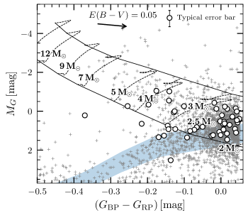
Figure 1: Gaia Hertzsprung-Russell diagram of candidate blue stars at high Galactic latitudes (grey cross symbols). The observed targets are shown as large circles. Solid curves represent the zero-age and terminal-age MS, while the evolutionary tracks for representative initial masses are plotted as dashed curves (Choi et al., 2016). The light-blue strip represents the horizontal branch (Dorman, 1992). The reddening vector and typical error bars of the observed targets are displayed at the top edge of the figure.

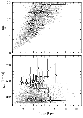
Figure 2: The relative parallax uncertainties and tangential velocities of early-type star candidates (cross symbols) and observed targets (circles with error bars) are plotted against the parallax-based distance in the top and bottom panels, respectively.

We queried the Gaia DR2 in order to identify candidate MS runaway stars with masses above 2 M_☉ at high Galactic latitudes ($|b|\geq 15^{\circ}$). We required that parallaxes are measured with a precision of better than 30%, and we applied color and absolute magnitude cuts of $G_{\rm BP}-G_{\rm RP}\leq 0.05$ mag and $M_{G}=G+5-5\log{(1000/\varpi)}\leq 3.7$ mag, respectively, where $G$, $G_{\rm BP}$, and $G_{\rm RP}$ are the Gaia magnitudes, and $\varpi$ is the parallax given in mas yr^-1. We filtered the Gaia photometry and astrometry, requiring high quality data as prescribed by Lindegren et al. (2018) and the Gaia Collaboration et al. (2018a). In addition, we requested that our selection had re-normalized unit weight error (ruwe) smaller than 1.4 (Lindegren, 2018). This procedure delivered 10 342 objects. The adql code used to perform our query is given in Appendix A.

We note that the $G$ magnitude distribution of the selected candidates is double peaked at $\approx 8.5$ and 14.5 mag, and that apparently brighter objects present relatively small tangential velocities in a heliocentric reference frame. In order to reduce contamination from objects that are less-likely runaway stars, we applied an additional cut defined via the tangential velocity as:

$$\varv_{\rm tan}=4.74\times\frac{\sqrt{{\mu^{*}_{\alpha}}^{2}+\mu_{\delta}^{2}}}{\varpi}\geq 150\,\mathrm{km}\,\mathrm{s}^{-1};$$ (1)

where $\mu^{*}_{\alpha}=\mu_{\alpha}\cos{\delta}$ and $\mu_{\delta}$ are the proper motion components along the right ascension and declination directions, respectively. This velocity cut delivers 2392 objects that are displayed in Fig. 1, along with the 48 stars for which we have collected follow-up spectroscopy.

Focusing on blue stars, our selection does not overlap with previous work (e.g. Hattori et al., 2018), which targeted cool stars for which six-dimensional data were delivered by Gaia DR2, including radial velocities that are not available for stars bluer than early-F spectral type, but also have their pitfalls (Boubert et al., 2019). Instead, we note that towards the lower edge of Fig. 1, i.e. the faint absolute magnitude cut, our candidates overlap with the hot subluminous star candidates identified by Geier et al. (2019), which we avoided as much as possible in our spectroscopic follow-up. In addition, we note that our target selection of blue stars at high Galactic latitudes would contain a large fraction of BHB stars and field blue stragglers (Brown et al., 2010) out of which we aim to disentangle MS runaway candidates.

3 Observations

The time allocation for our follow-up observations consisted of five nights at the New Technology Telescope (NTT) on 2019 August 15–20, with the ESO Faint Object Spectrograph and Camera (EFOSC2; Buzzoni et al., 1984).

Based on the on-sky visibility of suitable targets, we defined our priority list according to two empirical criteria. First, we favored objects having colors and absolute magnitudes that place them in the proximity of the unreddened MS (Fig. 1). Second, we covered a wide range of tangential velocities so not to solely favor stars with the highest apparent motion, as this quantity is negatively affected by larger parallax uncertainties (Fig. 2). Due to the time allocation in August, we observed 48 stars with right ascension between 16.5 h and 3 h. Figure 3 shows the spatial distribution of all the identified candidates and observed targets, which are compared to known runaway stars (Silva & Napiwotzki, 2011). The relevant Gaia data for the observed targets are listed in Table 1.

All the stars were observed with grism #7 and $2\times 2$ CCD binning, taking two exposures that ranged between 5–30 min, followed by one He-Ar arc exposure at the same position of the observed star. We typically observed three white dwarf flux standards per night (GD 50, LAWD 74, and LTT 7987). Our observations were undertaken near to full moon and the weather conditions were generally stable, frequently reaching sub-arcsec seeing; the sole exception was the first night, when thick clouds disrupted the second half of the night.

We used standard iraf (Tody, 1986, 1993) procedures for the reduction of long-slit spectra (Massey et al., 1992; Massey, 1997), which we bias subtracted, flat-field corrected, and wavelength and flux calibrated.

The observing setup delivered a useful spectral coverage between 3650$-$5050 Å, with a dispersion of $1.9$ Å/pixel (that translates to $\approx 120$ km s^-1 at H$\beta$). Because the point-spread-function of the spectral trace was smeared due to tracking limitations, the resolving power is strictly determined by the slit width. We measured a spectral resolution of $\Delta\lambda=6.5$ Å from the full width at half maximum of the He-Ar lines of the calibration lamp. The residuals of the wavelength solution have a root-mean-square of 0.2 Å. Given that no strong emission line from the night sky is detectable within the wavelength range of our spectra, we assessed the accuracy of the wavelength calibration by measuring the radial velocities of the white dwarf standards GD 50 and LTT 7987. Following the line-fitting technique adopted by Napiwotzki et al. (2020), we used their analysis software, fitsb2, to measure the radial velocity, $\varv_{\rm rad}$, of the white dwarf standards by iteratively combining synthetic spectra (Koester, 2010) with Gaussian and/or Lorentzian functions. From this procedure, we estimated an average systematic uncertainty of $\pm 25$ km s^-1 with respect to the values published by Napiwotzki et al. (2020), which we will add in quadrature to that obtained for the radial measurements of our science targets.

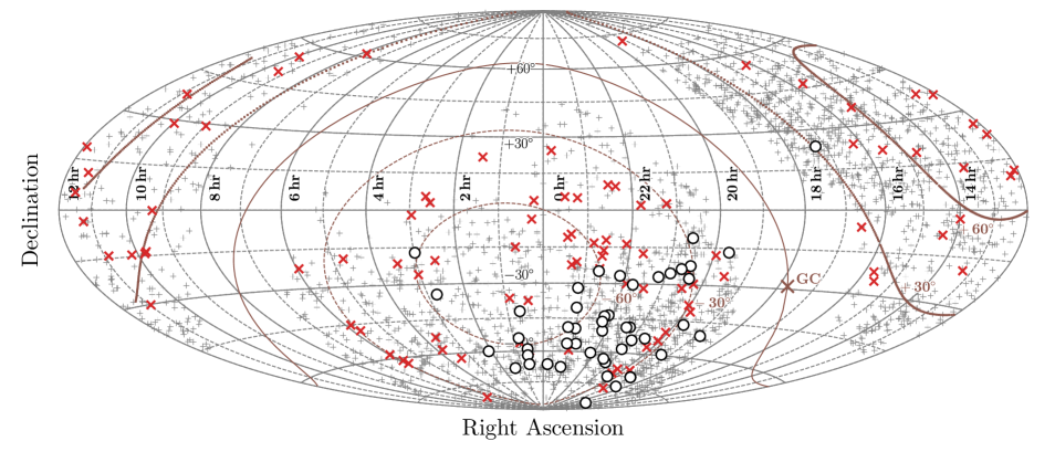
Figure 3: On-sky distribution of Gaia-selected candidate blue stars at high Galactic latitude (grey ’+’ symbols). The 48 observed targets (circles) and known MS runaway stars (red ’x’ symbols; Silva & Napiwotzki, 2011) are also shown.

Table 1: Gaia DR2 data for the observed 48 targets.

Gaia DR2	$\alpha$	$\delta$	$\mu^{*}_{\alpha}$	$\mu_{\delta}$	$\varpi$	$G$	$G_{\rm BP}$	$G_{\rm RP}$	Short name	Observing date
	(hms)	(dms)	(mas yr-1)	(mas yr-1)	(mas)	(mag)	(mag)	(mag)	(hhmm$\pm$ddmm)	(yyyy-mm-dd)
4907042024497066752	00:35:19.19	$-$59:00:22.35	$12.35\,\pm\,0.05$	$-8.92\,\pm\,0.04$	$0.12\pm 0.03$	14.47	14.46	14.44	0035$-$5900	2019-08-16
4901793883699014912	00:37:24.77	$-$61:54:55.17	$4.29\,\pm\,0.07$	$5.15\,\pm\,0.06$	$0.17\pm 0.04$	14.64	14.56	14.71	0037$-$6154	2019-08-20
4707068828231737856	00:38:16.76	$-$66:12:17.46	$21.22\,\pm\,0.05$	$-12.31\,\pm\,0.05$	$0.23\pm 0.03$	13.86	13.85	13.84	0038$-$6612	2019-08-16
4992937934442887296	00:39:20.74	$-$42:01:22.10	$20.70\,\pm\,0.04$	$-12.06\,\pm\,0.05$	$0.23\pm 0.04$	14.04	13.99	14.05	0039$-$4201	2019-08-16
4921153294167369856	00:49:49.34	$-$53:56:30.65	$20.97\,\pm\,0.04$	$-10.96\,\pm\,0.04$	$0.24\pm 0.03$	13.79	13.77	13.75	0049$-$5356	2019-08-16
4692515142570804608	01:22:35.90	$-$67:59:13.95	$17.26\,\pm\,0.07$	$-10.09\,\pm\,0.05$	$0.21\pm 0.03$	14.71	14.62	14.77	0122$-$6759	2019-08-16
4714790492235234176	02:05:56.74	$-$59:38:35.84	$6.14\,\pm\,0.07$	$2.11\,\pm\,0.06$	$0.15\pm 0.04$	13.07	12.97	13.15	0205$-$5938	2019-08-20
5050539802435511552	02:45:48.67	$-$34:18:56.36	$48.43\,\pm\,0.04$	$-9.93\,\pm\,0.06$	$0.51\pm 0.04$	12.41	12.40	12.36	0245$-$3418	2019-08-18
5153423785504601216	02:59:01.73	$-$17:04:59.96	$0.67\,\pm\,0.06$	$-6.63\,\pm\,0.07$	$0.17\pm 0.04$	13.58	13.52	13.63	0259$-$1705	2019-08-20
5768566765625082112	16:21:57.93	$-$83:50:56.96	$2.77\,\pm\,0.07$	$6.87\,\pm\,0.08$	$0.18\pm 0.04$	14.01	13.83	14.20	1621$-$8350	2019-08-20
4568776103982893056	17:15:28.48	+23:41:27.05	$1.39\,\pm\,0.04$	$-25.74\,\pm\,0.05$	$0.26\pm 0.03$	14.27	14.21	14.30	1715+2341	2019-08-18
6414065681237630720	18:39:12.47	$-$75:15:41.08	$-0.63\,\pm\,0.06$	$-16.08\,\pm\,0.09$	$0.20\pm 0.05$	16.03	15.95	16.09	1839$-$7515	2019-08-19
6655084093244687872	18:51:05.60	$-$50:36:39.75	$2.62\,\pm\,0.06$	$-10.83\,\pm\,0.06$	$0.16\pm 0.04$	15.04	15.01	15.01	1851$-$5036	2019-08-19
6421018924052925952	19:00:44.83	$-$70:32:03.13	$-12.38\,\pm\,0.04$	$-22.21\,\pm\,0.05$	$0.28\pm 0.03$	13.37	13.37	13.32	1900$-$7032	2019-08-18
6421018717894498048	19:00:33.66	$-$70:33:35.28	$5.70\,\pm\,0.05$	$-2.46\,\pm\,0.06$	$0.15\pm 0.04$	13.83	13.71	13.96	1900$-$7033	2019-08-20
6446292607565372800	19:19:54.92	$-$59:38:28.88	$5.21\,\pm\,0.06$	$-21.40\,\pm\,0.05$	$0.22\pm 0.05$	14.45	14.43	14.41	1919$-$5938	2019-08-17
4180161033474768640	19:39:22.50	$-$16:40:43.31	$1.43\,\pm\,0.11$	$-8.85\,\pm\,0.09$	$0.23\pm 0.05$	12.66	12.56	12.70	1939$-$1640	2019-08-19
6683685723576804992	19:44:12.51	$-$46:28:58.22	$-0.38\,\pm\,0.08$	$-36.87\,\pm\,0.07$	$0.30\pm 0.05$	13.32	13.19	13.40	1944$-$4628	2019-08-16
6374275970335856512	20:19:00.99	$-$71:07:53.49	$6.13\,\pm\,0.05$	$-37.38\,\pm\,0.06$	$0.39\pm 0.04$	12.74	12.72	12.71	2019$-$7107	2019-08-17
6846204709077343872	20:24:00.16	$-$27:25:25.22	$-11.54\,\pm\,0.07$	$-22.39\,\pm\,0.05$	$0.29\pm 0.04$	13.99	13.96	13.98	2024$-$2725	2019-08-18
6855907796113999872	20:28:33.90	$-$22:18:19.49	$-10.38\,\pm\,0.10$	$-28.60\,\pm\,0.06$	$0.31\pm 0.07$	12.38	12.37	12.33	2028$-$2218	2019-08-17
6901493616919722496	20:34:40.08	$-$11:08:05.94	$-13.81\,\pm\,0.10$	$-5.86\,\pm\,0.06$	$0.34\pm 0.06$	12.45	12.37	12.50	2034$-$1108	2019-08-19
6474092762640262016	20:34:20.66	$-$53:07:06.23	$-6.54\,\pm\,0.06$	$-18.68\,\pm\,0.06$	$0.19\pm 0.04$	13.43	13.41	13.40	2034$-$5307	2019-08-17
6854645866004127872	20:40:17.89	$-$23:36:47.22	$-23.18\,\pm\,0.07$	$-29.89\,\pm\,0.05$	$0.38\pm 0.04$	13.36	13.33	13.33	2040$-$2336	2019-08-17
6805531918539239040	20:54:36.95	$-$25:26:12.89	$-4.22\,\pm\,0.09$	$-5.34\,\pm\,0.05$	$0.18\pm 0.05$	13.43	13.33	13.52	2054$-$2526	2019-08-19
6470192756241354240	20:58:10.82	$-$54:07:33.00	$1.14\,\pm\,0.06$	$-28.15\,\pm\,0.06$	$0.29\pm 0.05$	13.11	13.10	13.05	2058$-$5407	2019-08-18
6456376915897827456	21:03:25.75	$-$58:15:35.28	$-15.18\,\pm\,0.06$	$-20.15\,\pm\,0.06$	$0.26\pm 0.04$	13.48	13.46	13.46	2103$-$5815	2019-08-18
6802706551612738432	21:10:28.12	$-$27:00:29.36	$-2.31\,\pm\,0.08$	$-25.71\,\pm\,0.05$	$0.27\pm 0.06$	13.28	13.28	13.23	2110$-$2700	2019-08-18
6401710125478435200	21:14:02.00	$-$64:38:47.32	$16.33\,\pm\,0.04$	$-17.01\,\pm\,0.04$	$0.24\pm 0.03$	13.97	13.93	13.98	2114$-$6438	2019-08-17
6479124127849108736	21:19:11.03	$-$48:27:17.63	$16.91\,\pm\,0.08$	$-11.78\,\pm\,0.06$	$0.21\pm 0.05$	14.53	14.51	14.47	2119$-$4827	2019-08-17
6467153298080614400	21:25:20.11	$-$48:34:50.08	$2.13\,\pm\,0.06$	$-19.70\,\pm\,0.06$	$0.19\pm 0.05$	14.11	14.09	14.09	2125$-$4834	2019-08-20
6403485802397156992	21:27:10.30	$-$63:00:27.09	$12.34\,\pm\,0.03$	$-16.52\,\pm\,0.04$	$0.17\pm 0.03$	13.86	13.85	13.81	2127$-$6300	2019-08-18
6593248963749480320	21:45:10.70	$-$30:22:26.73	$1.00\,\pm\,0.07$	$-25.95\,\pm\,0.07$	$0.25\pm 0.05$	13.66	13.64	13.63	2145$-$3022	2019-08-20
6619758674426791936	22:07:39.31	$-$26:45:05.56	$11.25\,\pm\,0.11$	$2.16\,\pm\,0.09$	$0.24\pm 0.07$	12.11	12.04	12.18	2207$-$2645	2019-08-19
6568272908586299136	22:07:29.23	$-$43:29:30.49	$17.90\,\pm\,0.04$	$-25.14\,\pm\,0.05$	$0.21\pm 0.04$	13.30	13.27	13.28	2207$-$4329	2019-08-19
6559602950163581952	22:07:25.53	$-$50:21:05.38	$-8.77\,\pm\,0.05$	$-26.38\,\pm\,0.07$	$0.28\pm 0.04$	13.72	13.69	13.69	2207$-$5021	2019-08-19
6409382345817774080	22:08:51.34	$-$60:26:11.43	$0.49\,\pm\,0.04$	$-12.51\,\pm\,0.06$	$0.27\pm 0.04$	13.82	13.74	13.86	2208$-$6026	2019-08-19
6568081112526763648	22:13:57.49	$-$43:57:43.72	$8.19\,\pm\,0.05$	$-11.90\,\pm\,0.06$	$0.29\pm 0.04$	13.67	13.59	13.73	2213$-$4357	2019-08-19
6566677242336303360	22:14:14.76	$-$46:20:06.71	$7.46\,\pm\,0.05$	$-16.93\,\pm\,0.06$	$0.17\pm 0.04$	14.77	14.71	14.79	2214$-$4620	2019-08-16
6623822705625945472	22:39:37.70	$-$24:55:02.94	$55.31\,\pm\,0.12$	$-24.94\,\pm\,0.12$	$0.59\pm 0.08$	12.50	12.42	12.59	2239$-$2455	2019-08-18
6505572880055200896	22:50:15.10	$-$56:25:17.08	$13.58\,\pm\,0.04$	$-16.19\,\pm\,0.04$	$0.15\pm 0.03$	14.42	14.41	14.38	2250$-$5625	2019-08-20
6514882651165295232	22:59:35.83	$-$49:31:18.23	$8.68\,\pm\,0.04$	$-27.30\,\pm\,0.06$	$0.27\pm 0.06$	14.29	14.28	14.27	2259$-$4931	2019-08-20
6543384947494107392	23:04:43.81	$-$40:21:07.52	$2.04\,\pm\,0.05$	$-5.30\,\pm\,0.06$	$0.14\pm 0.04$	13.89	13.86	13.87	2304$-$4021	2019-08-20
6556633886515772544	23:07:12.20	$-$31:57:38.11	$20.57\,\pm\,0.10$	$-9.06\,\pm\,0.07$	$0.35\pm 0.05$	12.30	12.24	12.36	2307$-$3157	2019-08-19
6493693515910526208	23:09:26.75	$-$56:23:02.24	$8.79\,\pm\,0.05$	$-9.18\,\pm\,0.06$	$0.32\pm 0.04$	13.53	13.47	13.56	2309$-$5623	2019-08-20
6391197660443817984	23:09:32.88	$-$67:29:14.43	$6.16\,\pm\,0.04$	$-23.25\,\pm\,0.05$	$0.20\pm 0.03$	13.72	13.70	13.70	2309$-$6729	2019-08-18
6503103617457504000	23:13:52.61	$-$48:58:15.92	$15.52\,\pm\,0.03$	$-10.51\,\pm\,0.04$	$0.19\pm 0.03$	14.09	14.08	14.04	2313$-$4858	2019-08-18
6389351133744091648	23:48:08.84	$-$66:12:17.59	$2.88\,\pm\,0.05$	$-9.08\,\pm\,0.05$	$0.15\pm 0.03$	15.41	15.38	15.40	2348$-$6612	2019-08-20

4 Data analysis

For the atmospheric characterization of the observed targets, we follow a three-step approach. First, we perform model fitting of their entire spectral energy distributions (SED) that consist of the available ground-based and space-borne broad-band photometry, from which we estimate the atmospheric parameters of each star, i.e., effective temperature and surface gravity, as well as the interstellar reddening and angular diameter ($T_{\rm eff}$, $\log{g}$, $E(44-55)$, and $\Theta$). Here, $E(44-55)$ is the monochromatic reddening measured at 4400 and 5500 Å, which is closely related to the more traditional band-integrated color excess $E(B-V)$, following the definition of Fitzpatrick et al. (2019). Second, we use the photometric estimates as initial guesses for the spectral analysis of flux calibrated spectra. Third, we re-determine $E(44-55)$ and $\Theta$, by employing the spectroscopic best-fit model in the SED-fitting procedure.

4.1 Grids of synthetic spectra

Due to the low resolution of the spectra in hand, only stellar parameters such as $T_{\rm eff}$ and $\log{g}$ can reliably be measured, while rotation, metallicity, and helium abundance are very poorly constrained, especially in the late-B/early-A spectral type transition, where many candidates are found. In this region of the Hertzsprung-Russell diagram, MS and BHB stars can not be distinguished on the basis of their atmospheric parameters alone (see Fig. 1), but additional information on the chemical composition and rotation of the stars is needed (see e.g. Heber et al., 2008b). Because the lack of spectral resolving power does not allow us to accurately obtain this auxiliary information, we perform the analysis of the SEDs and spectra for all targets twice by using two different grids of synthetic models, one being appropriate for MS stars and one being tailored to BHB stars, see below. The distinction between MS and BHB nature is then made based on the agreement of their spectrophotometric and parallax-based distances (see Sect. 4.4).

For MS stars it is self-evident to adopt a solar chemical composition. In contrast, the abundance patterns of BHB stars are diverse. Because the targets were selected to have high tangential velocities, BHB candidates are likely halo stars and thus metal poor. However, the stars’ chemical composition also varies along the horizontal branch. The morphology of BHBs of globular clusters reveals a universal discontinuity at $T_{\rm eff}\sim 11\,500$ K (Grundahl et al., 1999; Brown et al., 2016), which coincides with a drastic change in the chemical composition. While BHB stars cooler than 11 500K have the same metal content as the bulk of the stars of the host cluster, the abundance pattern of the hotter stars is peculiar, with helium depletion and iron enrichment (Behr, 2003). These chemical pecularities have been attributed to atomic diffusion, that is, to an interplay of gravitational settling and radiative levitation. The former leads to helium depletion and the latter causes the iron enrichment. The onset of atomic diffusion coincided with the disappearance of surface convection (Sweigart, 2002; Michaud et al., 2011). Because we can not determine the abundance pattern of the individual BHB stars, we calculate model atmospheres and synthetic spectra assuming a metalicity of one tenth solar for all BHB stars, but different helium abundances, that is, solar helium content for stars cooler than 11 500 K and 1/10 solar for the hotter ones.

Both grids span $T_{\rm eff}=7200$–$33\,000$ K and $\log{g}=3.0$–$4.6$. For $T_{\rm eff}\geq 9000$ K, we adopt the hybrid approach “ADS” (Przybilla et al., 2011; Irrgang et al., 2014), which combines Atlas12 (Kurucz, 1996) to compute hydrostatic model atmospheres in local thermodynamic equilibrium (LTE) with Detail (Giddings, 1981) to account for non-LTE effects; the Surface software (Giddings, 1981) is used to produce the synthetic spectrum. Another set of models, which extends below $10\,000$ K, has been generated by accounting only for LTE by means of the Atlas12 and synthe software (Kurucz, 1993). All models include the recent improvements introduced by Irrgang et al. (2018b) for the computation of level dissolution in proximity of the Balmer jump. The synthetic photometry is based on SEDs computed with Atlas12 using a ten times finer frequency grid, which were convolved with the appropriate transmission profile of each band-pass and subsequently shifted to the respective zero point.

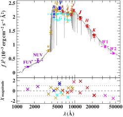
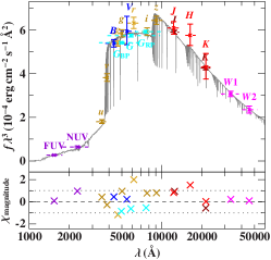
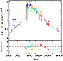
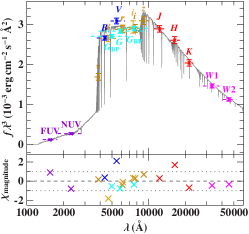
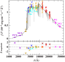
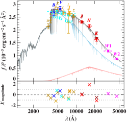
Figure 4: Examples for SED fits, from top left to bottom right: the MS candidates 0259$-$1705, 1900$-$7033, 2207$-$4329, and 2259$-$4931; the BHB candidate 1851$-$5036; and the binary 1944$-$4628. In each plot, the top panels show the measurements (color-coded by photometric system) as well as the best-fitting model spectra (gray), while the bottom panels show the error-normalized best-fit residuals, $\chi=(O_{i}-M_{i})/\sigma_{i}$, for each band-pass. The object 1944$-$4628 requires a composite SED fit, which is the combination of a $T_{\rm eff}\approx 24\,400$ K and a $T_{\rm eff}\approx 5900$ K component (blue and red curve, respectively).

4.2 SED fitting

We use the stilts software (Taylor, 2006) to query all the major photometric surveys that are available through the Table Access Protocol (TAP) of the VizieR online service (Ochsenbein, 2019), which is hosted by the Strasbourg Astronomical Data Center. For most of the stars, in addition to Gaia photometry, there is reliable coverage from the ultraviolet (GALEX; Bianchi et al., 2017) through the optical (APASS and SkyMapper; Henden et al., 2015; Wolf et al., 2018, as well as SDSS and PanSTARRS, for targets with $\delta\gtrsim-30$ deg; Alam et al. 2015; Chambers et al. 2016) and infrared (VHS, 2MASS, and WISE; McMahon et al., 2013; Skrutskie et al., 2006; Cutri & et al., 2014; Schlafly et al., 2019) We adopt the most recent calibration of GALEX (Wall et al., 2019), well-validated zero points and uncertainties for the other photometric surveys, as well as suggested corrections of Gaia DR2 photometry and the corresponding filter transmission profiles (Evans et al., 2018; Maíz Apellániz & Weiler, 2018).

The SED fitting procedure follows the methods outlined by Heber et al. (2018), allowing to directly estimate the four parameters: $\Theta$, $T_{\rm eff}$, $\log{g}$, and $E(44-55)$. We adopt the monochromatic extinction law by Fitzpatrick et al. (2019) with the total-to-selective extinction coefficient $R(55)=3.02$, as typical for the interstellar medium. The best-fit is found by matching observed and synthetic photometry via $\chi^{2}$ minimization. Each stellar SED is fitted with both model grids described in the previous section. Six examples are displayed in Fig. 4.

The preliminary SED fitting does not only provide an initial guess for the spectroscopic analysis, but is also crucial for identifying problematic objects like binary stars that exhibit composite SEDs. Indeed, we find that a single stellar component is not sufficient to model the SED of 1944$-$4628, which is likely an evolved low-mass star with an infrared excess due to a cooler binary companion (Fig. 4). Last but not least: photometric temperature estimates provide an important consistency check for our spectroscopic analysis, see the following section.

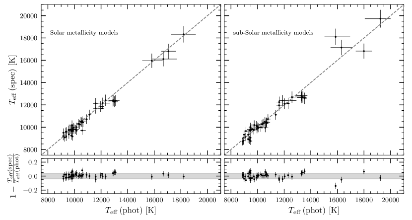
Figure 5: Comparisons between photometric $T_{\rm eff}$, measured via SED fitting, and spectroscopic $T_{\rm eff}$. The result for MS (top left panel) and BHB models (top right panel) are shown. The dashed lines represent the equality curves. The residuals are displayed as function of photometric $T_{\rm eff}$ in the lower panels. The gray shaded area represent the 4% systematic uncertainty assumed for the spectroscopic results.

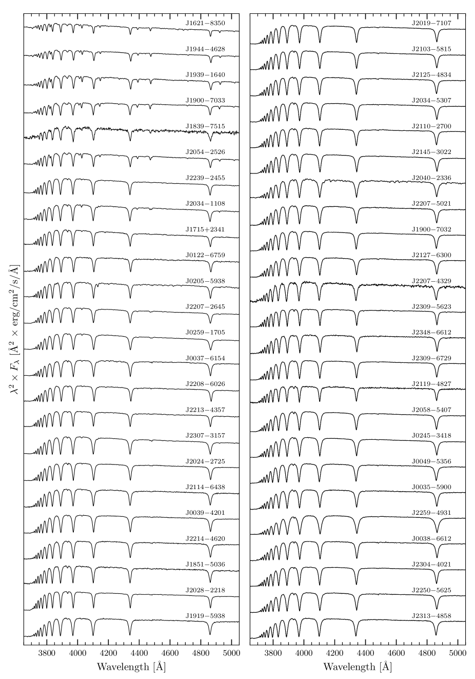
Figure 6: Observed spectra, sorted by decreasing $T_{\rm eff}$.

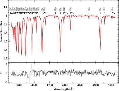
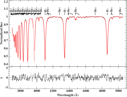
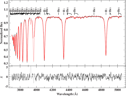
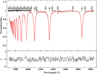
Figure 7: Examples of spectroscopic best-fits for four MS candidates (Sect. 4.4) with error-normalized residuals; from top left to bottom right: 1900$-$7033, 0259$-$1705, 2207$-$4329, and 2259$-$4931. The normalized spectra and the best-fit solar-metallicity models are shown in black and red, respectively. The two top panels show ADS models, while the bottom ones are obtained from the Atlas12/synthe grid. H and He lines are labeled at the corresponding wavelengths. The Ca ii lines are masked out during the fitting procedure due to possible interstellar contamination, which is recognizable in the spectrum of 1900$-$7033; masked regions are plotted using lighter colors. We note that the He i lines of 1900$-$7033 are stronger than those of our solar-metallicity model (c.f. Sect. 4.3 for a discussion on this star). The second star, 0259$-$1705, shows an excellent agreement between observed and model spectrum. In contrast, the Ca ii H lines of the two coolest stars in the bottom panels and the Mg ii 4481 line of 2259$-$4931 are weaker than those of the best-fit MS model. This issue, although to a lesser extent, also characterizes the best-fit obtained with sub-solar metallicity models.

4.3 Spectroscopic fitting

The analysis of flux-calibrated spectra follows the methods outlined by Irrgang et al. (2014), where the best-fits are determined via $\chi^{2}$ statistics through comparison with our model grids. We preferentially use ADS models, but we switch to the Atlas12/synthe grid in order to avoid extrapolation at the edge of the ADS grids. We ignore macroturbulence and assume a microturbulence of 2 km s^-1. As stated in Sect. 4.1, the low resolution of our spectra makes it difficult to measure detailed metal abundances and stellar rotation, hence, our approach is to fit the spectra with both the solar composition and the metal-deficient grids, respectively.

Mg and Si are the only elements for which the individual abundances are allowed to independently vary when using the ADS grids. However, we note that most measurements are poorly constrained and do not deliver reliable abundances, which is why we refrain from giving those numbers. Although we keep the projected rotational velocity, $\varv\sin{i}$, as a free parameter, it can be hardly resolved from our low-resolution spectra ($\Delta\varv\approx 400$ km s^-1). The spectra are corrected for the barycentric velocity and the radial velocity, $\varv_{\rm rad}$, is independently determined from each exposure. Statistical uncertainties affecting $T_{\rm eff}$ and $\log{g}$ are numerically inconspicuous. The systematic uncertainties dominating the error budget of $T_{\rm eff}$ and $\log{g}$ are estimated to the level of 4% and 0.1 dex, respectively. The error budget of $\varv_{\rm rad}$ is also dominated by systematic uncertainties, which are estimated from the difference between the measured values of the two available exposures for each star ($\lesssim 10$ km s^-1) and the 25 km s^-1 error, determined by comparing the $\varv_{\rm rad}$ of the white dwarf standards to values from the literature (Sect. 3).

The main results of our analysis are presented in Fig. 5, which displays the comparison between photometric and spectroscopic $T_{\rm eff}$ for the MS and BHB model analyses. The good agreement seen in Fig. 5 confirms the robustness of the SED and spectroscopic analyses, but also suggests that an additional method (like the distance comparison discussed in the following section) is necessary to distinguish between MS and BHB candidates.

Two stars, 1621$-$8350 and 1944$-$4628, are considerably hotter than the bulk of the sample, and are not included in Fig. 5. 1621$-$8350 is the only star that shows a He ii line (at 4685.8 Å) in its spectrum (Fig. 6), which leads to the classification of an O type star that is consistent with a high $T_{\rm eff}\approx 30\,000$ K. 1944$-$4628 is an early B-type star in a binary system (Fig. 4) at $T_{\rm eff}\approx 24\,400$ K. Both stars are discussed separately in Sect. 4.4.

A spectral atlas of our program stars is presented in Fig. 6, while examples of spectroscopic best-fits are shown in Fig. 7 for four stars (0259$-$1705, 1900$-$7033, 2207$-$4329, and 2259$-$4931) that are later classified as MS candidates based on their spectrophotometric distances (Sect. 4.4). In this figure, we exhibit three typical temperature regimes of our sample. We note that for hot stars like 1900$-$7033, shown in Fig. 7, and 1939$-$1640 and 2054$-$2526, it would be in fact possible to have more reliable He abundance measurements rather than assuming solar composition, but this exercises is beyond the scope of the paper. For cool objects like 2207$-$4329 and 2259$-$4931, we can see just a few weak metal lines. In these specific cases, both MS and BHB models seem to overestimate the intensity of the Ca ii H line, hinting at a sub-solar abundance that could be better investigated with higher-resolution spectra. The intensity of the Mg ii 4481 line of 2207$-$4329 is also overestimated. The star with an intermediate temperature, 0259$-$1705, shows an excellent agreement with the model.

Finally, we report that three stars were previously studied by other authors:

1900$-$7033: Kilkenny (1989) determined $T_{\rm eff}=18\,000$ K and $\log{g}=4.0$ with 10 % errors from 3 Å-resolution spectra, in agreement with our results. This author proposed the star to be mildly He-rich ($n$He/$n$H $\sim 0.3$). This finding is supported by our observations, because the He lines appear slightly deeper than those of the best-fit model with solar $\log{({\rm He/H})}=-1.01$ (see Fig. 7). Kilkenny (1989) also measured $\varv\sin{i}=175$ km s^-1 from the He lines, while the H$\gamma$ and H$\delta$ fits delivered smaller $\varv\sin{i}\approx 75$ and $100$ km s^-1, respectively. If we keep He as a free parameter, the best-fit result favors slightly super-solar He, but the line cores of the observed spectrum are still deeper than the model. Given that we cannot disentangle the effect of stellar rotation due to the low resolution of our spectra, we adopt the atmospheric parameters obtained for solar He abundance. Finally, Kilkenny (1989) reported a previous measurement of $\varv_{\rm rad}\approx-95$ km s^-1 that is at 2 $\sigma$ from our result.

2239$-$2455: Kilkenny (1987) used Strömgren photometry to classify this star as B7V, which is compatible with our spectral analysis. Ortiz et al. (2007) obtained 1.2 Å-resolution spectra over the H$\beta$–H$\epsilon$ spectral range, from which they suggest $T_{\rm eff}>17\,000$ K and $\log{g}=4.5\pm 0.5$ via measurements of equivalent widths and depths of the Balmer lines.

2307$-$3157: Ortiz et al. (2007) determined $T_{\rm eff}=8500$–10 000 K and $\log{g}=3$–3.5 with errors of 500 K and 0.5 dex, respectively, that roughly agree with our results.

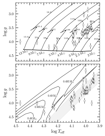
Figure 8: Kiel diagrams showing the atmospheric parameters of the observed stars as determined via the spectroscopic best-fit with model spectra representing MS and BHB stars (top and bottom panels, respectively). Top panel: Evolutionary tracks for rotating MS stars are plotted in black (Ekström et al., 2012). The initial masses of each model are noted below the zero-age MS (thick solid curve), while the stellar ages for selected evolutionary points along the tracks are given in mega years. Bottom panel: The horizontal branch is represented by the gray shaded area, and the evolutionary tracks for post-horizontal branch stars of different masses are drawn as solid curves (Dorman, 1992).

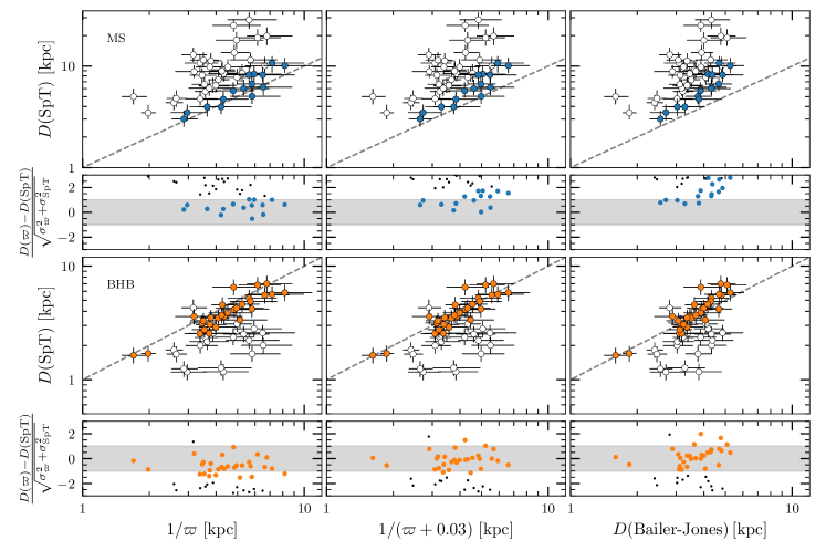
Figure 9: Comparison between spectrophotometric distances and three different parallax-based distance estimates. Upper panels: MS candidates (blue colored symbols) are identified via the 1 $\sigma$ agreement, which is represented by the dashed equality line and the shaded gray area. Lower panels: as for the upper panels, BHB candidates are represented by orange filled symbols. Note that three stars are classified both as MS and BHB candidates, hence they are color-colored in both the upper and lower panels.

4.4 Distance-driven classification and physical parameters

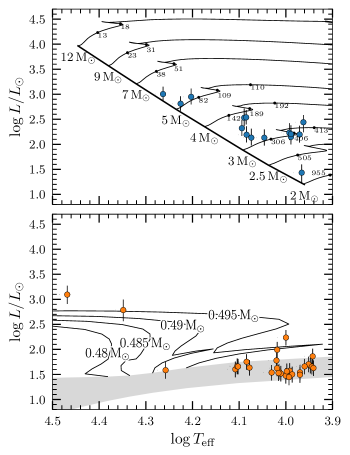
Figure 10: Theoretical Hertzsprung-Russell diagrams. The top panel shows our candidate MS stars over-plotted on Ekström et al. (2012) evolutionary tracks for rotating stars. The masses of each model are plotted in correspondence of the zero-age MS. The luminosities are derived by adopting the spectrophotometric distances. The bottom panel shows our candidate BHB stars over-plotted on the horizontal branch that is represented by a grey-shaded area and the evolutionary tracks for post-horizontal branch stars of given masses (Dorman, 1992; Dorman et al., 1993). Note that three stars are classified both as MS and BHB candidates, hence they feature in both panels with the appropriate parameters.

Figure 8 displays the $T_{\rm eff}$ and $\log{g}$ distribution of the observed stars in the Kiel diagram,as derived from the spectral analysis with synthetic spectra representing MS and BHB stars. For reference, we plot the theoretical evolutionary tracks for MS rotating stars (Ekström et al., 2012), and the horizontal branch and post-horizontal branch tracks (Dorman, 1992; Dorman et al., 1993). Given the degeneracy between MS stars of 3–4 M_☉ and BHB stars, whose evolutionary tracks overlap in the Kiel diagram, and the lack of additional information such as $\varv\sin{i}$ and metal abundances, it is a priori impossible to classify the majority of stars in our sample by just using $T_{\rm eff}$ and $\log{g}$.

Hence, to assess the nature of our program stars, we proceed in a different fashion, by comparing the Gaia parallaxes to the spectrophotometric distances, $D({\rm SpT})$, determined under the assumption that the observed stars are either MS or BHB stars. In order to estimate $D({\rm SpT})$ under the MS-star assumption, we first determine the stellar masses, radii, and luminosities via interpolation of the Ekström et al. (2012) tracks shown in Fig. 8 onto the $T_{\rm eff}$ and $\log{g}$ obtained via the spectroscopic fitting with the solar-metallicity grid. The spectrophotometric distance is then computed from the resulting stellar radius and the angular diameter determined via SED-fitting: $D({\rm SpT})=2R/\Theta$. In the BHB-star assumption, we assume a canonical BHB-star mass of $M=0.5\pm 0.1$ M_☉ from which we infer the stellar radius as $R=\sqrt{GM/g}$, where $G$ is the gravitational constant and $g$ is the surface gravity measured with the representative metal-poor model grid. Then, the $D({\rm SpT})$ is calculated as above using the appropriate $\Theta$.

Figure 9 displays the comparison between parallax-based distance estimators, $D(\varpi)$, and spectrophotometric distances for the MS and BHB results. The simplest estimator that we consider is $D(\varpi)=1/\varpi$, where $D(\varpi)$ is the median of the $1/\varpi$ distribution. We also consider the effect of a global zero-point shift of +0.03 mas, identified by Lindegren et al. (2018) from the analysis of an all-sky sample of extra-galactic sources – but these authors also noted that such an offset has relatively large variations over degree-wide scales. Finally, as advised by Bailer-Jones et al. (2018) and Luri et al. (2018), we also compare their prior-based distance estimate, $D$(Bailer-Jones), against $D({\rm SpT})$.

MS and BHB stars are expected to lie on the identity lines depicted in Fig. 9, when the $D({\rm SpT})$ computed from the corresponding models agree with the parallax-based distance estimates. From this comparison, we identify 15 MS candidates that have $D({\rm SpT})$ in agreement within 1 $\sigma$ with one of the three $D(\varpi)$ estimators (top panels of Fig. 9). The same comparisons for BHB estimates deliver 29 candidates (lower panels in Fig. 9). We note that three stars (0035$-$5900, 2127$-$6300, and 2304$-$4021) are both identified as MS and BHB candidates, while all the others are uniquely classified either as MS or BHB candidates. Among the 29 BHB candidates, there are 1621$-$8350 and 1944$-$4628 too, which we discuss in more detail below as evolved extreme horizontal branch stars (post-EHB). Seven stars of our sample do not fit in any of the two proposed classification schemes.

In general, we note that all MS candidates agree with the $1/\varpi$ estimator and that the other two estimators tend to bring the parallax-based distances closer to the Sun. This effect is more extreme for the $D$(Bailer-Jones) estimator of stars that have larger spectrophotometric distances, and it is also noticeable for the BHB candidates. The overlap between the MS and BHB candidates is limited to three stars, reinforcing the validity of this method. Nevertheless, this ambiguity and the presence of seven unclassified stars suggests the use of higher-resolution spectroscopy for future analysis in addition to improved parallaxes from future Gaia releases. Finally, we note that unclassified objects may point towards the presence of either unresolved binaries or other kinds of stars, like field blue stragglers (Brown et al., 2010) that we do not account for. Note that Brown et al. (2010) estimate that 74% of their blue halo star sample are BHBs and 26% are blue stragglers, which comes close to the 27 BHB stars versus 7 unclassified objects in our sample.

Table 3 lists the atmospheric parameters corresponding to the spectroscopic best-fit models implied by the unique distance-driven classification as MS/BHB candidates, along with the signal-to-noise ratio (S/N) of the stacked spectra and the $E(44-55)$. In passing, we note that the 7 unclassified stars cluster around $T_{\rm eff}\approx 10\,000$ K and $\log{g}=3.6$. For the remainder of the manuscript, we take a conservative approach by considering as runaway MS candidates at high Galactic latitudes the 12 stars that uniquely agree within 1 $\sigma$ of the identity line in either of the top panels of Fig. 9, assuming the three stars with ambiguous classification as BHB candidates.

The spectra of the two hottest stars previously mentioned (1621$-$8350 and 1944$-$4628) resemble those of MS objects of late O- and early B-type (see Fig. 6). However, the respective spectroscopic distances would be about 30 and 10 kpc, which is at variance with their Gaia parallaxes (top panels of Fig. 9). Therefore, they must be evolved low-mass stars that mimic hot massive stars. Such stars are rare but do exist, e.g., the B-type star HZ 22 of $T_{\rm eff}=29\,200$ K and $\log{g}=4.04$ (Saffer et al., 1997) and the O-type star PG2 120+062 (Moehler et al., 1994). HZ 22, in fact, is a binary orbited by an unseen white dwarf, which allowed its mass to be estimated at 0.39 M_☉ (Schönberner, 1978). Hence, those stars are likely post-RGB or post-AGB stars. For a brief account of such so-called UV-bright stars see also Heber (2016).

While the SED of 1621$-$8350 can be matched by a single hot star model, this is not the case for 1944$-$4628, which shows an infrared excess indicative of a cool companion (Fig. 4). Adding a grid of SEDs from Husser et al. (2013), the infrared excess can well be matched by a composite model SED that includes a companion of $T_{\rm eff}$ = 5900${}^{+1300}_{-1200}$ K with a radius of 1.34${}^{+0.60}_{-0.35}$ R_⊙. Although uncertainties are large, the derived radius and luminosity of the companion are consistent with those of a G-type MS star.

We list the physical parameters of the 12 MS candidates in Table LABEL:t:ms. The physical parameters of the 27 BHB candidates as well as those of the two post-EHB candidates and the late-type companion of 1944$-$4628 are given in Table 4.4.

To conclude this section, we present the results of our classification in the two theoretical Hertzsprung-Russell diagrams of Fig. 10, displaying the MS and BHB candidates with their appropriate evolutionary tracks. A few MS candidates appear to be fairly evolved, with evolutionary timescales, $\tau_{\rm evo}$, in the range of 300–400 Myr. The BHB candidates are mostly distributed along their main locus. From Fig. 8–10, we conclude that the positions of 1621$-$8350 and 1944$-$4628 are well matched by the evolution of EHB stars (subluminous B stars) after core helium exhaustion (Dorman et al., 1993).

Table 2: Spectroscopic parameters of the sample derived from model spectra, as appropriate for their classification (MS or BHB candidate, respectively). Unclassified stars are listed at the bottom with their parameters derived from models with sub-solar composition.

Short name	S/N	$T_{\rm eff}$	$\log{g}$	$\varv_{\rm rad}$	$E(44-55)$	MS
		(K)	$\log{({\rm cm\,s}^{-2})}$	(km s-1)	(mag)
0035$-$5900	180	$8900$	3.19	$141\,\pm\,31$	$0.02\,\pm\,0.02$	✓✗
0037$-$6154	230	$11\,900$	4.05	$138\,\pm\,26$	$<\,0.01$	✓
0038$-$6612	220	$8900$	3.18	$233\,\pm\,26$	$<\,0.01$	✗
0039$-$4201	220	$10\,300$	3.58	$144\,\pm\,25$	$<\,0.02$	✗
0049$-$5356	240	$9300$	3.42	$-109\,\pm\,26$	$<\,0.02$	✗
0122$-$6759	140	$12\,800$	3.91	$272\,\pm\,27$	$<\,0.01$	✗
0205$-$5938	380	$12\,300$	3.81	$109\,\pm\,27$	$0.00$	✓
0245$-$3418	370	$9300$	3.47	$123\,\pm\,28$	$<\,0.06$	✗
0259$-$1705	370	$12\,100$	4.07	$185\,\pm\,26$	$0.04\,\pm\,0.02$	✓
1621$-$8350a	210	$29\,400$	4.00	$115\,\pm\,39$	$0.08\,\pm\,0.02$	✗
1715+2341	190	$12\,700$	3.83	$1\,\pm\,26$	$0.04\,\pm\,0.02$	✗
1839$-$7515	50	$18\,100$	4.53	$65\,\pm\,26$	$0.12\,\pm\,0.03$	✗
1851$-$5036	120	$10\,500$	3.38	$-28\,\pm\,26$	$0.05\,\pm\,0.03$	✗
1900$-$7032	340	$9800$	3.58	$-46\,\pm\,28$	$0.05\,\pm\,0.04$	✓✗
1900$-$7033	250	$16\,800$	4.19	$-38\,\pm\,26$	$0.02\,\pm\,0.02$	✓
1919$-$5938	160	$10\,300$	3.61	$-88\,\pm\,25$	$0.06\,\pm\,0.04$	✗
1939$-$1640	200	$18\,300$	4.20	$224\,\pm\,26$	$0.12\,\pm\,0.01$	✓
1944$-$4628a,b	260	$22\,300$	4.02	$261\,\pm\,26$	$0.16\,\pm\,0.02$	✗
2019$-$7107	320	$10\,100$	3.60	$109\,\pm\,26$	$0.05\,\pm\,0.03$	✓✗
2024$-$2725	180	$10\,700$	3.67	$123\,\pm\,26$	$0.05\,\pm\,0.03$	✗
2028$-$2218	380	$10\,000$	2.84	$79\,\pm\,25$	$0.05\,\pm\,0.03$	✗
2034$-$1108	250	$12\,400$	4.00	$-74\,\pm\,28$	$0.02\,\pm\,0.02$	✓
2034$-$5307	280	$9800$	3.61	$123\,\pm\,28$	$0.04\,\pm\,0.03$	✓
2054$-$2526	220	$16\,000$	3.97	$65\,\pm\,26$	$0.05\,\pm\,0.02$	✓
2110$-$2700	270	$9800$	3.48	$-3\,\pm\,33$	$0.06\,\pm\,0.03$	✗
2114$-$6438	160	$10\,400$	3.53	$17\,\pm\,28$	$0.02\,\pm\,0.02$	✗
2119$-$4827	120	$10\,400$	3.16	$27\,\pm\,25$	$0.10\,\pm\,0.03$	✗
2125$-$4834	230	$10\,000$	3.61	$8\,\pm\,26$	$0.04\,\pm\,0.03$	✗
2145$-$3022	280	$9700$	3.53	$179\,\pm\,27$	$0.04\,\pm\,0.04$	✗
2207$-$2645	340	$12\,200$	3.78	$51\,\pm\,26$	$0.02\,\pm\,0.02$	✓
2207$-$4329	150	$9700$	3.62	$-170\,\pm\,26$	$0.02\,\pm\,0.02$	✓
2207$-$5021	190	$9800$	3.61	$75\,\pm\,26$	$0.03\,\pm\,0.03$	✗
2208$-$6026	250	$12\,000$	3.76	$356\,\pm\,25$	$<\,0.03$	✗
2213$-$4357	250	$12\,100$	3.67	$64\,\pm\,29$	$<\,0.01$	✗
2214$-$4620	160	$10\,400$	3.62	$112\,\pm\,26$	$0.01\,\pm\,0.01$	✗
2239$-$2455	320	$12\,700$	3.83	$-43\,\pm\,29$	$<\,0.01$	✗
2250$-$5625	220	$8800$	3.20	$118\,\pm\,26$	$<\,0.01$	✗
2259$-$4931	250	$9200$	4.16	$244\,\pm\,27$	$<\,0.01$	✓
2307$-$3157	320	$11\,100$	3.94	$-2\,\pm\,29$	$0.01\,\pm\,0.01$	✓
2313$-$4858	210	$8700$	3.22	$-183\,\pm\,29$	$<\,0.01$	✗
2348$-$6612	130	$10000$	3.51	$225\,\pm\,26$	$<\,0.04$	✗
2040$-$2336	260	$10\,200$	3.92	$56\,\pm\,26$	$0.05\,\pm\,0.03$
2058$-$5407	300	$9700$	3.60	$-8\,\pm\,30$	$0.06\,\pm\,0.03$
2103$-$5815	300	$10\,000$	3.60	$121\,\pm\,27$	$0.03\,\pm\,0.03$
2127$-$6300	220	$9100$	3.26	$99\,\pm\,26$	$<\,0.03$
2304$-$4021	300	$8800$	2.99	$27\,\pm\,27$	$0.00$
2309$-$5623	340	$9900$	3.21	$186\,\pm\,27$	$0.00$
2309$-$6729	290	$9800$	3.52	$126\,\pm\,32$	$0.02\,\pm\,0.02$

Table 3: Physical parameters of the MS candidates: mass, radius, luminosity, age, and spectrophotometric distance.

Short name	$M$/M☉	$R$/R☉	$\log{L/{\rm L}_{\sun}}$	$\tau_{\rm evo}$	$D$(SpT)
				(Myr)	(kpc)
0037$-$6154	$3.17^{+0.32}_{-0.17}$	$2.77^{+0.54}_{-0.40}$	$2.13^{+0.18}_{-0.15}$	$213^{+28}_{-79}$	$8.34^{+1.80}_{-1.30}$
0205$-$5938	$3.91^{+0.38}_{-0.29}$	$4.07^{+0.79}_{-0.64}$	$2.53^{+0.19}_{-0.17}$	$152^{+25}_{-22}$	$6.19^{+1.35}_{-1.05}$
0259$-$1705	$3.42^{+0.24}_{-0.21}$	$2.83^{+0.51}_{-0.43}$	$2.19^{+0.17}_{-0.15}$	$148^{+57}_{-66}$	$5.04^{+0.98}_{-0.80}$
1900$-$7033	$5.04^{+0.36}_{-0.25}$	$3.00^{+0.54}_{-0.44}$	$2.81^{+0.15}_{-0.14}$	$38^{+20}_{-24}$	$8.19^{+1.57}_{-1.25}$
1939$-$1640	$5.81^{+0.36}_{-0.35}$	$3.16^{+0.55}_{-0.47}$	$3.00^{+0.15}_{-0.15}$	$27^{+16}_{-20}$	$4.72^{+0.86}_{-0.73}$
2034$-$1108	$3.58^{+0.28}_{-0.24}$	$3.14^{+0.58}_{-0.48}$	$2.32^{+0.17}_{-0.16}$	$165^{+26}_{-36}$	$3.48^{+0.68}_{-0.56}$
2034$-$5307	$3.00^{+0.37}_{-0.11}$	$4.51^{+0.94}_{-0.60}$	$2.23^{+0.19}_{-0.14}$	$317^{+48}_{-59}$	$6.01^{+1.34}_{-0.85}$
2054$-$2526	$5.21^{+0.48}_{-0.36}$	$3.91^{+0.74}_{-0.60}$	$2.95^{+0.17}_{-0.15}$	$63^{+9}_{-13}$	$8.22^{+1.68}_{-1.33}$
2207$-$2645	$3.90^{+0.26}_{-0.21}$	$4.20^{+0.75}_{-0.62}$	$2.54^{+0.15}_{-0.14}$	$171^{+23}_{-21}$	$3.96^{+0.75}_{-0.61}$
2207$-$4329	$2.97^{+0.31}_{-0.12}$	$4.45^{+0.88}_{-0.60}$	$2.21^{+0.17}_{-0.14}$	$329^{+50}_{-58}$	$5.71^{+1.21}_{-0.81}$
2259$-$4931	$2.17^{+0.18}_{-0.20}$	$2.03^{+0.38}_{-0.33}$	$1.43^{+0.16}_{-0.21}$	$462^{+160}_{-212}$	$3.97^{+0.80}_{-0.79}$
2307$-$3157	$3.15^{+0.29}_{-0.24}$	$3.14^{+0.60}_{-0.49}$	$2.13^{+0.17}_{-0.16}$	$236^{+26}_{-36}$	$3.01^{+0.61}_{-0.49}$

Table 4: Physical parameters of BHB and post-EHB candidates computed adopting the atmospheric parameters derived from metal deficient atmospheric models and a mass of $M=0.5\pm 0.1$ M_☉. The two hot post-EHB stars are listed at the end. 1944$-$4628B denotes the cool companion of 1944$-$4628.

Short name	$R$/R☉	$\log{L/{\rm L}_{\sun}}$	$D$(SpT)
			(kpc)
0035$-$5900	$2.94^{+0.48}_{-0.44}$	$1.68^{+0.15}_{-0.16}$	$5.84^{+1.03}_{-0.92}$
0038$-$6612	$2.97^{+0.48}_{-0.44}$	$1.70^{+0.15}_{-0.16}$	$4.54^{+0.78}_{-0.70}$
0039$-$4201	$1.88^{+0.31}_{-0.29}$	$1.56^{+0.15}_{-0.16}$	$3.61^{+0.62}_{-0.55}$
0049$-$5356	$2.28^{+0.37}_{-0.34}$	$1.54^{+0.15}_{-0.16}$	$3.48^{+0.58}_{-0.53}$
0122$-$6759	$1.29^{+0.21}_{-0.20}$	$1.60^{+0.15}_{-0.16}$	$4.15^{+0.70}_{-0.64}$
0245$-$3418	$2.15^{+0.36}_{-0.32}$	$1.50^{+0.15}_{-0.16}$	$1.70^{+0.28}_{-0.26}$
1715+2341	$1.41^{+0.23}_{-0.21}$	$1.67^{+0.15}_{-0.16}$	$3.51^{+0.59}_{-0.54}$
1839$-$7515	$0.63^{+0.12}_{-0.10}$	$1.59^{+0.17}_{-0.17}$	$4.27^{+0.79}_{-0.68}$
1851$-$5036	$2.37^{+0.38}_{-0.35}$	$1.78^{+0.15}_{-0.16}$	$6.82^{+1.12}_{-1.01}$
1900$-$7032	$1.88^{+0.31}_{-0.28}$	$1.47^{+0.15}_{-0.16}$	$2.35^{+0.40}_{-0.35}$
1919$-$5938	$1.83^{+0.30}_{-0.27}$	$1.52^{+0.15}_{-0.16}$	$3.87^{+0.64}_{-0.58}$
2019$-$7107	$1.84^{+0.30}_{-0.28}$	$1.50^{+0.15}_{-0.16}$	$1.83^{+0.30}_{-0.28}$
2024$-$2725	$1.71^{+0.28}_{-0.26}$	$1.54^{+0.15}_{-0.16}$	$3.16^{+0.52}_{-0.49}$
2028$-$2218	$4.41^{+0.71}_{-0.66}$	$2.24^{+0.15}_{-0.16}$	$3.61^{+0.59}_{-0.55}$
2110$-$2700	$2.13^{+0.35}_{-0.31}$	$1.57^{+0.15}_{-0.16}$	$2.56^{+0.43}_{-0.38}$
2114$-$6438	$1.99^{+0.34}_{-0.30}$	$1.62^{+0.15}_{-0.16}$	$3.69^{+0.63}_{-0.56}$
2119$-$4827	$3.04^{+0.53}_{-0.45}$	$1.99^{+0.16}_{-0.16}$	$6.51^{+1.14}_{-0.98}$
2125$-$4834	$1.84^{+0.31}_{-0.28}$	$1.48^{+0.15}_{-0.16}$	$3.38^{+0.56}_{-0.51}$
2145$-$3022	$2.01^{+0.33}_{-0.30}$	$1.50^{+0.15}_{-0.16}$	$2.91^{+0.49}_{-0.44}$
2207$-$5021	$1.83^{+0.31}_{-0.28}$	$1.45^{+0.15}_{-0.16}$	$2.76^{+0.47}_{-0.42}$
2208$-$6026	$1.54^{+0.25}_{-0.23}$	$1.64^{+0.15}_{-0.16}$	$3.06^{+0.52}_{-0.47}$
2213$-$4357	$1.70^{+0.28}_{-0.25}$	$1.75^{+0.15}_{-0.16}$	$3.29^{+0.55}_{-0.50}$
2214$-$4620	$1.81^{+0.30}_{-0.27}$	$1.53^{+0.15}_{-0.16}$	$4.89^{+0.83}_{-0.74}$
2239$-$2455	$1.41^{+0.23}_{-0.21}$	$1.66^{+0.15}_{-0.16}$	$1.64^{+0.27}_{-0.24}$
2250$-$5625	$2.91^{+0.48}_{-0.44}$	$1.65^{+0.15}_{-0.16}$	$5.58^{+0.99}_{-0.90}$
2313$-$4858	$2.87^{+0.48}_{-0.43}$	$1.63^{+0.15}_{-0.16}$	$4.61^{+0.84}_{-0.73}$
2348$-$6612	$2.04^{+0.35}_{-0.32}$	$1.56^{+0.16}_{-0.17}$	$7.02^{+1.22}_{-1.11}$
1621$-$8350a	$1.16^{+0.20}_{-0.18}$	$3.09^{+0.18}_{-0.19}$	$5.22^{+0.92}_{-0.82}$
1944$-$4628a	$1.14^{+0.19}_{0.17}$	2.46 ${}^{+0.16}_{-0.16}$	$2.56^{+0.44}_{-0.38}$
1944$-$4628Ba	1.34${}^{+0.60}_{-0.35}$	-0.06 ${}^{+0.68}_{-0.90}$

5 Galactic orbit simulation

To model the trajectories of our MS candidates in the Milky Way’s gravitational potential, we use the python package galpy for galactic dynamics (Bovy, 2015). We adopt the Model I potential of Irrgang et al. (2013), which is implemented in galpy in a simplified fashion that serves our purposes. This potential is a revised version of that described by Allen & Santillan (1991). The Sun is located at $R_{\sun}=8.4$ kpc from the Galactic center, around which it orbits with $\varv_{0}=242$ km s^-1. The local escape velocity is $\varv_{\sun,\,{\rm esc}}=614.4$ km s^-1. We note that the galpy reference potential, MWPotential2014, accounts for a lower-mass Galactic halo model that, however, has relatively small impact in determining the past trajectories of the youngest and nearest runaway candidates in our sample. The mass of the Milky Way’s halo can be relevant for the study of unbound stars, as we discuss in the following section.

The past and future trajectories of the runaway candidates are determined in a statistical fashion, as we randomly sample the observed quantities ($\alpha$, $\delta$, $\mu^{*}_{\alpha}$, $\mu_{\delta}$, $D(\rm SpT)$, $\varv_{\rm rad}$) by adopting their uncertainties and relevant correlations. We draw 10 000 initial conditions, which are evolved for 10 Gyr in the future and traced back in the past for sufficiently large time (i.e. up to $\tau_{\rm evo}$). For each star, we note the rest-frame velocity, $\varv_{\rm rf}$, the past and future Galactic cartesian coordinates, and the corresponding velocity components. We estimate the escape probability from the Milky Way, $P_{\rm esc}$, for each star as the fraction of initial conditions where $(\varv_{\rm rf}-\varv_{\rm esc})>0$. We determine the vertical component of the angular momentum, $L_{Z}$, which indicates the direction towards which the star has been ejected. We also numerically estimate the eccentricity, $e$, the median orbital apocenter and pericenter, $R_{\rm apo}$ and $R_{\rm peri}$, and the maximum vertical displacement, $Z_{\rm max}$. The most recent Galactic plane crossings, $R(Z=0)$, are recorded and used to determine the flight time from such locations, $\tau_{\rm flight}$. The ejection velocity, $V_{\rm ej}$, is determined as the velocity possessed by the star at $R(Z=0)$, corrected for the solar motion and the Galactic rotation.

Table 5 lists the relevant orbital quantities for the 12 MS runaway candidates in a Galactocentric reference system that is left-handed, i.e., with the $x$- and $y$-axis pointing, respectively, from the Milky Way’s center towards the Sun and along the direction of the Galactic rotation.

Table 5: Orbital parameters of our MS candidates.

Short name	$X$	$Y$	$Z$	$\varv_{Z}$	$\varv_{\rm rf}$	$P_{\rm esc}$	$e$	$L_{Z}$	$R_{\rm peri}$	$R_{\rm apo}$	$Z_{\rm max}$	$R(Z=0)$	$\varv_{\rm ej}$	$\tau_{\rm flight}$
	(kpc)	(kpc)	(kpc)	(km s-1)	(km s-1)			(kpc km s-1)	(kpc)	(kpc)	(kpc)	(kpc)	(km s-1)	(Myr)
0037$-$6154	$5.63^{+0.50}_{-0.53}$	$-3.86^{+0.70}_{-0.74}$	$-6.82^{+1.24}_{-1.31}$	$-231^{+31}_{-32}$	$380^{+42}_{-38}$	$0.0$	$0.7$	$2100$	$8.24^{+0.91}_{-0.62}$	$40.6^{+29.0}_{-15.0}$	$31.5^{+25.0}_{-12.7}$	$8.9^{+1.6}_{-1.1}$	$330^{+31}_{-37}$	$24^{+3}_{-3}$
0205$-$5938	$7.40^{+0.19}_{-0.20}$	$-3.41^{+0.66}_{-0.67}$	$-5.07^{+0.98}_{-1.00}$	$-61^{+22}_{-23}$	$194^{+18}_{-12}$	$0.0$	$0.4$	$1300$	$4.81^{+0.88}_{-0.66}$	$11.49^{+1.86}_{-1.36}$	$6.17^{+1.71}_{-1.28}$	$5.2^{+0.7}_{-0.5}$	$273^{+84}_{-47}$	$37^{+6}_{-6}$
0259$-$1705	$10.85^{+0.43}_{-0.43}$	$-0.93^{+0.16}_{-0.16}$	$-4.30^{+0.76}_{-0.76}$	$-178^{+22}_{-23}$	$204^{+18}_{-16}$	$0.0$	$0.2$	$1000$	$7.90^{+0.75}_{-0.66}$	$12.65^{+1.10}_{-0.83}$	$11.22^{+1.64}_{-1.69}$	$10.5^{+0.7}_{-0.6}$	$276^{+27}_{-27}$	$21^{+4}_{-4}$
1900$-$7033	$2.43^{+1.01}_{-1.03}$	$-4.23^{+0.72}_{-0.73}$	$-3.60^{+0.61}_{-0.63}$	$-183^{+37}_{-38}$	$363^{+30}_{-28}$	$0.0$	$0.5$	$1300$	$5.77^{+0.60}_{-0.23}$	$19.41^{+9.36}_{-5.21}$	$15.20^{+9.70}_{-5.72}$	$7.9^{+1.0}_{-0.8}$	$295^{+25}_{-39}$	$16^{+1}_{-1}$
1939$-$1640	$4.27^{+0.69}_{-0.69}$	$1.75^{+0.29}_{-0.29}$	$-1.44^{+0.24}_{-0.25}$	$-166^{+19}_{-19}$	$340^{+25}_{-25}$	$0.0$	$0.5$	$1100$	$4.12^{+0.19}_{-0.11}$	$11.79^{+3.10}_{-2.33}$	$6.77^{+1.60}_{-1.23}$	$5.9^{+0.6}_{-0.6}$	$259^{+23}_{-23}$	$8^{+0}_{-1}$
2034$-$1108	$5.87^{+0.45}_{-0.45}$	$1.74^{+0.31}_{-0.31}$	$-1.62^{+0.29}_{-0.29}$	$188^{+29}_{-29}$	$253^{+28}_{-24}$	$0.0$	$0.4$	$900$	$3.64^{+0.31}_{-0.27}$	$9.15^{+1.63}_{-1.06}$	$6.19^{+1.62}_{-1.30}$	$3.8^{+0.4}_{-0.3}$	$409^{+30}_{-42}$	$93^{+19}_{-13}$
2034$-$5307	$3.75^{+0.83}_{-0.83}$	$-1.22^{+0.22}_{-0.22}$	$-3.57^{+0.64}_{-0.64}$	$102^{+35}_{-36}$	$339^{+96}_{-94}$	$0.0$	$0.5$	$-1200$	$4.89^{+0.06}_{-0.45}$	$14.0^{+21.0}_{-6.6}$	$9.1^{+18.4}_{-5.2}$	$13.2^{+15.0}_{-6.3}$	$371^{+63}_{-48}$	$68^{+45}_{-19}$
2054$-$2526	$2.30^{+1.09}_{-1.12}$	$2.28^{+0.42}_{-0.41}$	$-4.98^{+0.89}_{-0.92}$	$48^{+22}_{-22}$	$221^{+25}_{-21}$	$0.0$	$0.3$	$700$	$3.85^{+1.15}_{-0.68}$	$7.75^{+1.51}_{-0.75}$	$6.48^{+1.73}_{-1.37}$	$6.9^{+1.7}_{-1.2}$	$262^{+16}_{-17}$	$50^{+11}_{-7}$
2207$-$2645	$6.26^{+0.36}_{-0.37}$	$0.95^{+0.16}_{-0.16}$	$-3.17^{+0.54}_{-0.55}$	$-152^{+28}_{-29}$	$342^{+25}_{-23}$	$0.0$	$0.6$	$1600$	$4.41^{+0.72}_{-0.66}$	$20.36^{+5.25}_{-3.63}$	$9.56^{+3.61}_{-2.71}$	$4.4^{+0.7}_{-0.6}$	$272^{+47}_{-44}$	$16^{+1}_{-1}$
2207$-$4329	$5.00^{+0.60}_{-0.60}$	$-0.26^{+0.05}_{-0.05}$	$-4.57^{+0.81}_{-0.81}$	$-50^{+41}_{-40}$	$638^{+140}_{-138}$	$0.4$	…	$-2300$	$6.78^{+0.18}_{-2.06}$	$...$	$...$	$16.5^{+5.9}_{-5.4}$	$802^{+129}_{-115}$	$32^{+4}_{-3}$
2259$-$4931	$6.50^{+0.37}_{-0.38}$	$-0.73^{+0.14}_{-0.15}$	$-3.38^{+0.67}_{-0.68}$	$-114^{+28}_{-30}$	$350^{+93}_{-82}$	$0.0$	$0.5$	$-2100$	$7.25^{+0.03}_{-0.06}$	$20.9^{+33.5}_{-10.8}$	$11.2^{+19.0}_{-4.9}$	$9.0^{+2.8}_{-1.0}$	$541^{+40}_{-54}$	$22^{+6}_{-5}$
2307$-$3157	$7.26^{+0.21}_{-0.21}$	$0.30^{+0.05}_{-0.06}$	$-2.77^{+0.51}_{-0.51}$	$-101^{+34}_{-33}$	$230^{+40}_{-32}$	$0.0$	$0.9$	$200$	$0.63^{+0.69}_{-0.48}$	$12.92^{+3.13}_{-1.93}$	$6.17^{+5.33}_{-2.35}$	$2.0^{+1.4}_{-1.2}$	$469^{+170}_{-106}$	$18^{+2}_{-2}$

6 Properties of the runaway candidates

6.1 Orbit analysis

As expected for nearby runaway MS stars, all but one candidate are bound to the Milky Way’s potential, since they have $\varv_{\rm rf}$ that is on average two times smaller than $\varv_{\rm esc}$ at their Galactic coordinates. The only exceptions is 2207$-$4329 that has an escape probability $P_{\rm esc}=0.4$, defined as the fraction of simulated trajectories with $\varv_{\rm rest}>\varv_{\rm esc}$.

Due to our selection cut of $\varv_{\rm tan}>150$ km s^-1 (Eq. 1), all stars in our sample (both the MS and BHB candidates) resulted to have $|\varv_{\rm rad}|\lesssim\varv_{\rm tan}$ within the error bars. Three stars, 2034$-$5307, 2207$-$4329, and 2259$-$4931, have the largest $\varv_{\rm tan}\gtrsim 450$ km s^-1 of all MS candidates. This unusual feature can be also noted in the Toomre diagram of Fig. 11, where the three stars have large negative Galactic cartesian $V$ components (i.e. they lag behind the Milky Way’s rotation), as it is more typically seen for the majority of BHB candidates in our sample. The remaining MS candidates, instead, have moderate tangential velocities of $\varv_{\rm tan}\simeq 200$ km s^-1. The mostly retrograde motions of the BHB stars implies that they belong to the halo population. In the future, additional runaway candidates could be selected on the basis of their location in the Galactic Cartesian velocity space, as depicted by the Toomre diagram (Fig. 11).

Following the general direction of the Galactic rotation most MS candidates have $L_{Z}>0$ kpc km s^-1, with the exception of the three more extreme stars that have large negative, Cartesian velocity $V$ components. While our distance-based method entirely classify them as MS stars, these three stars appear to possess kinematics that are more typical of BHB stars. We note that 2034$-$5307 and 2207$-$4329 have $T_{\rm eff}$ and $\log{g}$ in the overlapping region of MS tracks and the horizontal branch (Fig. 8). Instead, 2259$-$4931 has a larger $\log{g}$ that excludes a BHB nature. As already mentioned in Sect. 4, our distance-based method identifies MS candidates for which we envisage higher-resolution spectroscopy for a more detailed assessment of their nature.

All the MS candidates are found below the Galactic plane and are currently moving away from it, with the exception of three stars, 2034$-$1108, 2034$-$5307, and 2054$-$2526, that are approaching the plane. The orbits of the observed runaway candidates cover a wide range of eccentricities, $e=0.2$–0.9, that is larger than the typical values for thin disc stars. All the runaway candidates have their orbital apocenters roughly between the solar circle and $R_{\rm apo}=20$ kpc, with a few exceptions potentially reaching out to very far Galactic radii. Their orbits are typically enclosed within $Z_{\rm max}=4$–40 kpc from the Galactic plane.

The trajectories of 2307$-$3157 have their orbital pericenters relatively close to the Galactic center ($R_{\rm peri}<1$ kpc); hence, its motion could be affected by the shape and orientation of the Galactic bar, which is not accounted for in our Galactic potential model. The trajectories of stars reaching beyond $R_{\rm apo}\gtrsim 20$ kpc, instead, might experience gravitational perturbations due to the Large Magellanic Cloud (Kenyon et al., 2018; Erkal et al., 2019a), which our Galactic model also does not account for.

Finally, we do not list the orbital parameters ($e$, $R_{\rm peri}$, $R_{\rm apo}$, and $Z_{\rm max}$) of 2207$-$4329 in Table 5, for they are unconstrained due to its non-zero probability of escaping the Milky Way. For this star, a significant fraction of simulated trajectories reaches extremely large Galatocentric radii without returning back, within the 10 Gyr time-frame of our simulation. As for the other stars, the parallax uncertainty has a major role in determining the agreement with the spectrophotometric distance and its classification as MS candidate. For the time being, we note that the adopted potential (Model I of Irrgang et al., 2013) delivers a $\varv_{\sun,\,{\rm esc}}$ that is already a few tens of km s^-1 larger than more recent Gaia-based estimates (Monari et al., 2018; Deason et al., 2019), suggesting a real chance for this star to escape the Milky Way if confirmed as MS candidate.

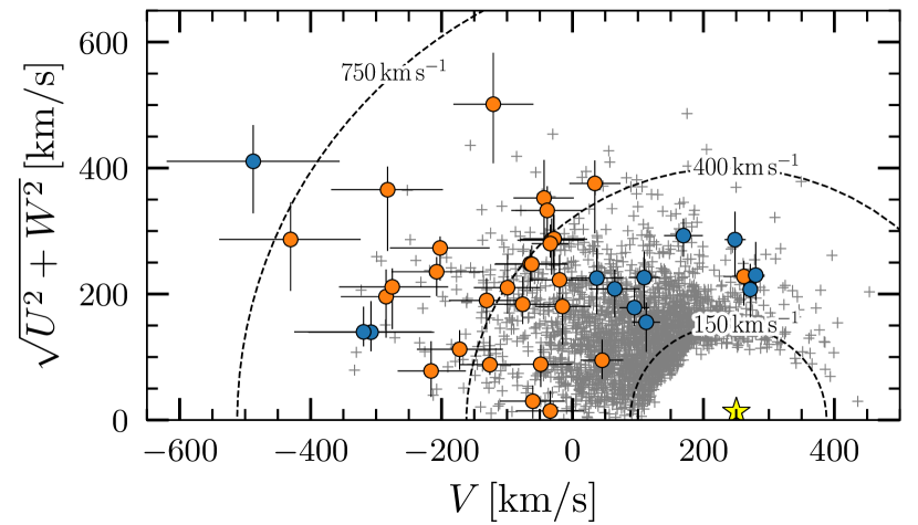
Figure 11: The positions of the program stars in the Toomre diagram. The quantity $V$ is the velocity component in direction of Galactic rotation, $U$ towards the Galactic center, and $W$ perpendicular to the Galactic plane. The local standard of rest (LSR) is marked by a yellow asterisk. The dashed circles centered around the LSR represent boundaries for three restframe velocities. The observed stars are plotted with error bars. Blue symbols correspond to MS candidates, while orange symbols are used for the BHB stars. All the targets identified in Sect. 2 are plotted as gray crosses, adopting $\varv_{\rm rad}=0$ km s^-1.

6.2 Birth place and flight times

The birth places of B-type MS stars are open clusters and associations within the thin disc of the Milky Way. Although short compared to that of lower mass stars, the MS life of late-B and early-A type stars can span from several 10 Myr up to $\sim 1$ Gyr, making the identification of their birth places a relatively complex issue.

In Sect. 5, we have determined the most recent crossings of the Galactic plane for the MS candidates, from which we estimate the flight times. To confirm the runaway hypothesis, the flight times need to be shorter than the ages estimated from evolutionary tracks ($\tau_{\rm flight}\leq\tau_{\rm evo}$). In the case of ejection via the binary supernova mechanism, a runaway star could be rejuvenated due to mass-transfer prior to the core-collapse explosion of the primary (Schneider et al., 2015); hence, it could even appear slightly younger than the flight time.

In Fig. 12, we show the comparison between these two quantities, noting that – within the error bars – all the candidates are below or overlap with the solid curve representing the identity line. Two thirds of our runaway candidates have ages that are more than 2 times longer than the flight times. This result poses the question of whether the reported crossing locations of the Galactic plane, $R(Z=0)$, identify the real birth places and flight times. In fact, we note that all candidates with $\tau_{\rm evo}>100$ Myr, with the exclusion of 2207$-$4329, could have crossed the Galactic plane two or more times in the past. If the mechanisms that caused their runaway status occurred early in their lifetime, as it is generally accepted for the binary supernova and dynamical ejection scenarios, the most recent $R(Z=0)$ do not constrain their $\tau_{\rm flight}$.

The various ejection mechanisms have intrinsic timescales. For example, the canonical binary ejection mechanism necessarily occurs on very short timescales of a few Myr, which are driven by the core-collapse supernova (Portegies Zwart, 2000), and the dynamical ejection from clusters can produce runaway stars for several hundred Myr (Moyano Loyola & Hurley, 2013). Therefore, future intermediate- and high-resolution spectroscopy would enable an improved understanding, e.g. via the detection of polluting elements from supernova ejecta (Pan et al., 2012) as found for the hyper-runaway giant HD 271971 (Przybilla et al., 2008) or via the comparison of measured abundances with the average elemental abundances of specific locations in the Galactic disc (Irrgang et al., 2010).

Of all MS candidates, the possibly unbound runaway, 2207$-$4329, also has the Galactic plane crossing radius that is the furthest from the Galactic center at $R(Z=0)=16.5^{+5.9}_{-5.4}$. Such a large distance is similar to the case of HD 271791 also originating from the outer Galactic disk (Heber et al., 2008a; Przybilla et al., 2008), the ejection velocity of which, however, is much lower ($390\pm 4$ km s^-1; Irrgang et al., 2019). If the MS classification of 2207$-$4329 is confirmed by future Gaia data releases and higher-resolution spectroscopy, alternative birth places above the Galactic plane (e.g. the tidal stream of a satellite galaxy colliding with the Milky Way; Abadi et al., 2009) or other exotic scenarios involving intermediate-mass black holes (Fragione & Gualandris, 2019) should also be investigated.

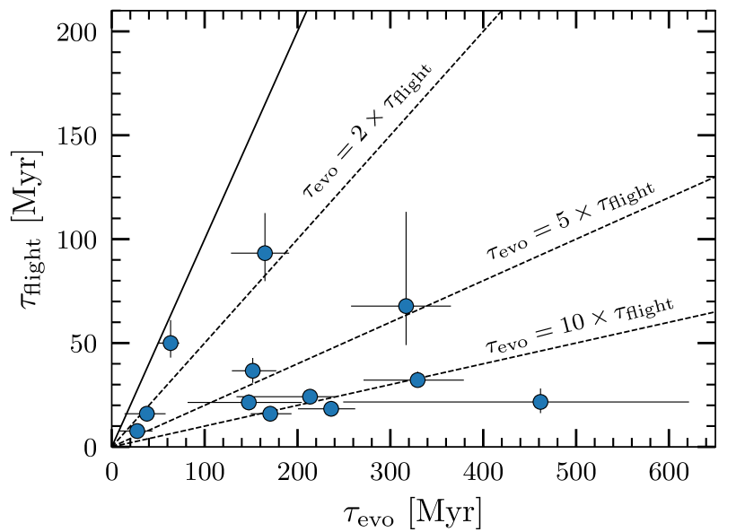
Figure 12: Comparison of flight times and stellar ages for the runaway MS candidates. The solid line represents the identity curve. The dashed lines mark the ranges where $\tau_{\rm evo}=2,\,5$, and 10 times $\tau_{\rm flight}$.

6.3 Ejection velocity distribution

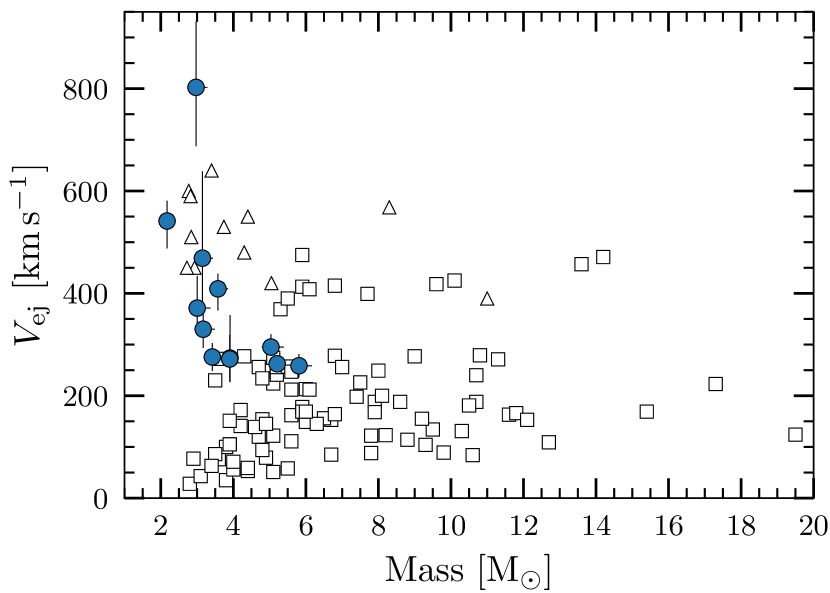
Figure 13: Ejection velocities of runaway stars are plotted against their masses. Our 12 MS runaway candidates are represented by blue circles with error bars (note that two stars have very similar masses and, thus, overlapping symbols). The runaway stars studied by Silva & Napiwotzki (2011) are plotted as squares. More recently discovered high-velocity runaway stars as listed by Irrgang et al. (2019) are plotted as triangles, with masses updated from Kreuzer et al. (2020) when available.

Silva & Napiwotzki (2011) described the relation between stellar mass and ejection velocity, with reference to their compiled sample of runaway stars, as mostly determined by the binary supernova mechanism. They also noted that the dynamical ejection from clusters could contribute to the low-ejection velocity population. On the contrary, the fastest runaway stars could have an overlap with the slowest hyper-velocity stars.

In Fig. 13, our runaway candidates occupy a lower mass range with respect to the Silva & Napiwotzki (2011) and Irrgang et al. (2019) samples. The increase of ejection velocities towards lower masses that characterize our sample appears to be in agreement with the predictions for binary supernova ejections in the most extreme scenarios (Tauris, 2015; Evans et al., 2020). However, Renzo et al. (2019) suggest that the dominant fraction of runaway stars with large ejection velocities could be mostly formed via dynamical interactions in open clusters, or more exotic scenarios. Interestingly, the ejection velocities of three runaway candidates, 2207$-$4329, 2259$-$4931, and 2307$-$3157, could largely exceed $400$–$500$ km s^-1, which would be challenging the classical runaway scenarios (Irrgang et al., 2018a, 2019). Of the three stars, 2207$-$4329 is by far the fastest (802${}^{+129}_{-115}$ km s^-1). 2259$-$4931, which is the least massive star of our sample, is the second fastest one, ejected at 541${}^{+40}_{-54}$ km s^-1 from near the solar circle. If confirmed as a MS star, 2207$-$4329 would be the fastest known hyper-runaway star (cf. Table 5 of Irrgang et al., 2019). Its ejection velocity would exceed that of HVS 5 (640${}^{+50}_{-40}$ km s^-1; Irrgang et al., 2019), even when we allow for the rather large uncertainty of the former. 2259$-$4931 would also gain a prominent position in the list of Galactic disc runaways with the largest ejection velocities, next to the well studied PG 1610+062 (550$\pm$20 km s^-1).

7 Conclusions

We have presented the selection of bright early-type MS candidates at high Galactic latitudes, relying on the Gaia DR2 astrometry and photometry, with the goal of identifying new runaway stars. To test our selection we have followed-up 48 stars obtaining low-resolution optical spectroscopy. By comparing spectrophotometric distances and parallax-based distance estimators, we propose 12 stars as MS candidates. Of the remaining stars, 27 are likely BHB stars, two are rare highly evolved hot stars, and seven yet unclassified stars could be binaries or blue stragglers.

The newly identified runaway candidates are mostly found within the 2–4 M_☉ range. We numerically trace the past trajectories of these stars, identifying their nearest Galactic disc crossings locations, flight times, and ejection velocities. Most stars have ejection velocities between 200–450 km s^-1. Three stars exceed the 450 km s^-1 upper limit of classical ejection scenarios (see Irrgang et al., 2019) such as the binary supernova mechanism and dynamical ejection from open clusters and, thus, call for a yet unknown ejection process (see also Evans et al., 2020). One of the three stars has a non-negligible escape probability, but more precise and accurate astrometry is required to check whether they are bound to the Galaxy. According to their kinematics the BHB stars belong to the halo population.

We remark that high-resolution spectroscopy is crucial to asses precise rotational velocities and abundances, which are necessary to confirm the MS nature of these candidates and shed light on their ejection mechanisms and birth places. We also envisage an improved kinematic analysis and stellar classification of the wider target lists, arising from the future Gaia data releases. More accurate and precise parallaxes will make it possible to extend the current volume beyond $\sim$10 kpc, which is currently limited by the parallax precision and accuracy.

Appendix A Gaia archive query

We performed the following query via the online service offered by the Astronomisches Rechen-Institut of the Heidelberg University:

SELECT *
FROM gaiadr2.gaia_source
WHERE parallax_error/parallax<=0.3
   AND parallax  > 0
   AND phot_g_mean_mag + 5 -
       5*log10(1000/parallax)<= 3.7
   AND ABS(b)>=15 AND bp_rp<=0.05
   AND phot_bp_rp_excess_factor
       <= 1.3 + 0.06*power(bp_rp,2)
   AND phot_bp_rp_excess_factor
       >= 1.0 + 0.015*power(bp_rp,2)
   AND visibility_periods_used >= 8
   AND phot_g_mean_flux_over_error >= 50
   AND phot_bp_mean_flux_over_error >= 20
   AND phot_rp_mean_flux_over_error >= 20
   AND ruwe <= 1.4

In addition, we filtered the data with the prescription of Eq.1.

References

- Abadi et al. (2009) Abadi, M. G., Navarro, J. F., & Steinmetz, M. 2009, ApJ, 691, L63
- Alam et al. (2015) Alam, S., Albareti, F. D., Allende Prieto, C., et al. 2015, ApJS, 219, 12
- Allen & Santillan (1991) Allen, C. & Santillan, A. 1991, Rev. Mexicana Astron. Astrofis., 22, 255
- Bailer-Jones et al. (2018) Bailer-Jones, C. A. L., Rybizki, J., Fouesneau, M., Mantelet, G., & Andrae, R. 2018, AJ, 156, 58
- Behr (2003) Behr, B. B. 2003, ApJS, 149, 67
- Bianchi et al. (2017) Bianchi, L., Shiao, B., & Thilker, D. 2017, ApJS, 230, 24
- Blaauw (1961) Blaauw, A. 1961, Bull. Astron. Inst. Netherlands, 15, 265
- Boubert et al. (2018) Boubert, D., Guillochon, J., Hawkins, K., et al. 2018, MNRAS, 479, 2789
- Boubert et al. (2019) Boubert, D., Strader, J., Aguado, D., et al. 2019, MNRAS, 486, 2618
- Bovy (2015) Bovy, J. 2015, ApJS, 216, 29
- Brown et al. (2016) Brown, T. M., Cassisi, S., D’Antona, F., et al. 2016, ApJ, 822, 44
- Brown (2015) Brown, W. R. 2015, ARA&A, 53, 15
- Brown et al. (2010) Brown, W. R., Geller, M. J., Kenyon, S. J., & Diaferio, A. 2010, AJ, 139, 59
- Brown et al. (2018) Brown, W. R., Lattanzi, M. G., Kenyon, S. J., & Geller, M. J. 2018, ApJ, 866, 39
- Buzzoni et al. (1984) Buzzoni, B., Delabre, B., Dekker, H., et al. 1984, The Messenger, 38, 9
- Casagrande et al. (2019) Casagrande, L., Wolf, C., Mackey, A. D., et al. 2019, MNRAS, 482, 2770
- Chambers et al. (2016) Chambers, K. C., Magnier, E. A., Metcalfe, N., et al. 2016, arXiv e-prints, arXiv:1612.05560
- Choi et al. (2016) Choi, J., Dotter, A., Conroy, C., et al. 2016, ApJ, 823, 102
- Cutri & et al. (2014) Cutri, R. M. & et al. 2014, VizieR Online Data Catalog, II/328
- Deason et al. (2019) Deason, A. J., Fattahi, A., Belokurov, V., et al. 2019, MNRAS, 485, 3514
- Dorman (1992) Dorman, B. 1992, ApJS, 80, 701
- Dorman et al. (1993) Dorman, B., Rood, R. T., & O’Connell, R. W. 1993, ApJ, 419, 596
- Edelmann et al. (2005) Edelmann, H., Napiwotzki, R., Heber, U., Christlieb, N., & Reimers, D. 2005, ApJ, 634, L181
- Ekström et al. (2012) Ekström, S., Georgy, C., Eggenberger, P., et al. 2012, A&A, 537, A146
- Erkal et al. (2019a) Erkal, D., Belokurov, V., Laporte, C. F. P., et al. 2019a, MNRAS, 487, 2685
- Erkal et al. (2019b) Erkal, D., Boubert, D., Gualandris, A., Evans, N. W., & Antonini, F. 2019b, MNRAS, 483, 2007
- Evans et al. (2018) Evans, D. W., Riello, M., De Angeli, F., et al. 2018, A&A, 616, A4
- Evans et al. (2020) Evans, F. A., Renzo, M., & Rossi, E. M. 2020, MNRAS, 497, 5344
- Fitzpatrick et al. (2019) Fitzpatrick, E. L., Massa, D., Gordon, K. D., Bohlin, R., & Clayton, G. C. 2019, ApJ, 886, 108
- Fragione & Gualandris (2019) Fragione, G. & Gualandris, A. 2019, MNRAS, 489, 4543
- Gaia Collaboration et al. (2018a) Gaia Collaboration, Babusiaux, C., van Leeuwen, F., et al. 2018a, A&A, 616, A10
- Gaia Collaboration et al. (2018b) Gaia Collaboration, Brown, A. G. A., Vallenari, A., et al. 2018b, A&A, 616, A1
- Gaia Collaboration et al. (2016) Gaia Collaboration, Prusti, T., de Bruijne, J. H. J., et al. 2016, A&A, 595, A1
- Geier et al. (2019) Geier, S., Raddi, R., Gentile Fusillo, N. P., & Marsh, T. R. 2019, A&A, 621, A38
- Giddings (1981) Giddings, J. R. 1981, PhD thesis
- González-Fernández et al. (2018) González-Fernández, C., Hodgkin, S. T., Irwin, M. J., et al. 2018, MNRAS, 474, 5459
- Grundahl et al. (1999) Grundahl, F., Catelan, M., Landsman, W. B., Stetson, P. B., & Andersen, M. I. 1999, ApJ, 524, 242
- Gvaramadze et al. (2009) Gvaramadze, V. V., Gualandris, A., & Portegies Zwart, S. 2009, MNRAS, 396, 570
- Hattori et al. (2018) Hattori, K., Valluri, M., Bell, E. F., & Roederer, I. U. 2018, ApJ, 866, 121
- Heber (2016) Heber, U. 2016, PASP, 128, 082001
- Heber et al. (2008a) Heber, U., Edelmann, H., Napiwotzki, R., Altmann, M., & Scholz, R. D. 2008a, A&A, 483, L21
- Heber et al. (2008b) Heber, U., Hirsch, H. A., Edelmann, H., et al. 2008b, in Astronomical Society of the Pacific Conference Series, Vol. 392, Hot Subdwarf Stars and Related Objects, ed. U. Heber, C. S. Jeffery, & R. Napiwotzki, 167
- Heber et al. (2018) Heber, U., Irrgang, A., & Schaffenroth, J. 2018, Open Astronomy, 27, 35
- Henden et al. (2015) Henden, A. A., Levine, S., Terrell, D., & Welch, D. L. 2015, in American Astronomical Society Meeting Abstracts, Vol. 225, American Astronomical Society Meeting Abstracts #225, 336.16
- Hewett et al. (2006) Hewett, P. C., Warren, S. J., Leggett, S. K., & Hodgkin, S. T. 2006, MNRAS, 367, 454
- Hills (1988) Hills, J. G. 1988, Nature, 331, 687
- Holberg & Bergeron (2006) Holberg, J. B. & Bergeron, P. 2006, AJ, 132, 1221
- Hoogerwerf et al. (2001) Hoogerwerf, R., de Bruijne, J. H. J., & de Zeeuw, P. T. 2001, A&A, 365, 49
- Husser et al. (2013) Husser, T. O., Wende-von Berg, S., Dreizler, S., et al. 2013, A&A, 553, A6
- Irrgang et al. (2019) Irrgang, A., Geier, S., Heber, U., Kupfer, T., & Fürst, F. 2019, A&A, 628, L5
- Irrgang et al. (2018a) Irrgang, A., Kreuzer, S., & Heber, U. 2018a, A&A, 620, A48
- Irrgang et al. (2018b) Irrgang, A., Kreuzer, S., Heber, U., & Brown, W. 2018b, A&A, 615, L5
- Irrgang et al. (2014) Irrgang, A., Przybilla, N., Heber, U., et al. 2014, A&A, 565, A63
- Irrgang et al. (2010) Irrgang, A., Przybilla, N., Heber, U., Nieva, M. F., & Schuh, S. 2010, ApJ, 711, 138
- Irrgang et al. (2013) Irrgang, A., Wilcox, B., Tucker, E., & Schiefelbein, L. 2013, A&A, 549, A137
- Jarrett et al. (2011) Jarrett, T. H., Cohen, M., Masci, F., et al. 2011, ApJ, 735, 112
- Kenyon et al. (2018) Kenyon, S. J., Bromley, B. C., Brown, W. R., & Geller, M. J. 2018, ApJ, 864, 130
- Kilkenny (1987) Kilkenny, D. 1987, MNRAS, 228, 713
- Kilkenny (1989) Kilkenny, D. 1989, MNRAS, 238, 955
- Koester (2010) Koester, D. 2010, Mem. Soc. Astron. Italiana, 81, 921
- Koposov et al. (2020) Koposov, S. E., Boubert, D., Li, T. S., et al. 2020, MNRAS, 491, 2465
- Kreuzer et al. (2020) Kreuzer, S., Irrgang, A., & Heber, U. 2020, A&A, 637, A53
- Kurucz (1993) Kurucz, R. L. 1993, SYNTHE spectrum synthesis programs and line data
- Kurucz (1996) Kurucz, R. L. 1996, Astronomical Society of the Pacific Conference Series, Vol. 108, Status of the ATLAS 12 Opacity Sampling Program and of New Programs for Rosseland and for Distribution Function Opacity, ed. S. J. Adelman, F. Kupka, & W. W. Weiss, 160
- Lindegren (2018) Lindegren, L. 2018, Re-normalising the astrometric chi-square in Gaia DR2, Tech. Rep. GAIA-C3-TN-LU-LL-124-01, Lund Observatory, Lund, Sweden
- Lindegren et al. (2018) Lindegren, L., Hernández, J., Bombrun, A., et al. 2018, A&A, 616, A2
- Luri et al. (2018) Luri, X., Brown, A. G. A., Sarro, L. M., et al. 2018, A&A, 616, A9
- Maíz Apellániz et al. (2018) Maíz Apellániz, J., Pantaleoni González, M., Barbá, R. H., et al. 2018, A&A, 616, A149
- Maíz Apellániz & Weiler (2018) Maíz Apellániz, J. & Weiler, M. 2018, A&A, 619, A180
- Massey (1997) Massey, P. 1997
- Massey et al. (1992) Massey, P., Valdes, F., & Barnes, J. 1992
- McMahon et al. (2013) McMahon, R. G., Banerji, M., Gonzalez, E., et al. 2013, The Messenger, 154, 35
- Michaud et al. (2011) Michaud, G., Richer, J., & Richard, O. 2011, A&A, 529, A60
- Moehler et al. (1994) Moehler, S., Heber, U., & Dreizler, S. 1994, A&A, 282, L29
- Monari et al. (2018) Monari, G., Famaey, B., Carrillo, I., et al. 2018, A&A, 616, L9
- Moyano Loyola & Hurley (2013) Moyano Loyola, G. R. I. & Hurley, J. R. 2013, MNRAS, 434, 2509
- Napiwotzki et al. (2020) Napiwotzki, R., Karl, C. A., Lisker, T., et al. 2020, A&A, 638, A131
- Ochsenbein (2019) Ochsenbein, F. 2019, The VizieR database of astronomical catalogues
- Oh & Kroupa (2016) Oh, S. & Kroupa, P. 2016, A&A, 590, A107
- Ortiz et al. (2007) Ortiz, R., Malacarne, M., Wilhelm, R., et al. 2007, AJ, 134, 1183
- Pan et al. (2012) Pan, K.-C., Ricker, P. M., & Taam, R. E. 2012, ApJ, 750, 151
- Perets & Šubr (2012) Perets, H. B. & Šubr, L. 2012, ApJ, 751, 133
- Pérez & Granger (2007) Pérez, F. & Granger, B. E. 2007, Computing in Science and Engineering, 9, 21
- Portegies Zwart (2000) Portegies Zwart, S. F. 2000, ApJ, 544, 437
- Poveda et al. (1967) Poveda, A., Ruiz, J., & Allen, C. 1967, Boletin de los Observatorios Tonantzintla y Tacubaya, 4, 86
- Przybilla et al. (2008) Przybilla, N., Fernanda Nieva, M., Heber, U., & Butler, K. 2008, ApJ, 684, L103
- Przybilla et al. (2011) Przybilla, N., Nieva, M.-F., & Butler, K. 2011, in Journal of Physics Conference Series, Vol. 328, Journal of Physics Conference Series, 012015
- Raddi et al. (2018) Raddi, R., Hollands, M. A., Gänsicke, B. T., et al. 2018, MNRAS, 479, L96
- Raddi et al. (2019) Raddi, R., Hollands, M. A., Koester, D., et al. 2019, MNRAS, 489, 1489
- Renzo et al. (2019) Renzo, M., Zapartas, E., de Mink, S. E., et al. 2019, A&A, 624, A66
- Saffer et al. (1997) Saffer, R. A., Keenan, F. P., Hambly, N. C., Dufton, P. L., & Liebert, J. 1997, ApJ, 491, 172
- Schlafly et al. (2019) Schlafly, E. F., Meisner, A. M., & Green, G. M. 2019, ApJS, 240, 30
- Schneider et al. (2015) Schneider, F. R. N., Izzard, R. G., Langer, N., & de Mink, S. E. 2015, ApJ, 805, 20
- Schönberner (1978) Schönberner, D. 1978, A&A, 70, 451
- Shen et al. (2018) Shen, K. J., Boubert, D., Gänsicke, B. T., et al. 2018, ApJ, 865, 15
- Silva & Napiwotzki (2011) Silva, M. D. V. & Napiwotzki, R. 2011, MNRAS, 411, 2596
- Skrutskie et al. (2006) Skrutskie, M. F., Cutri, R. M., Stiening, R., et al. 2006, AJ, 131, 1163
- Sweigart (2002) Sweigart, A. V. 2002, Highlights of Astronomy, 12, 292
- Tauris (2015) Tauris, T. M. 2015, MNRAS, 448, L6
- Taylor (2006) Taylor, M. B. 2006, Astronomical Society of the Pacific Conference Series, Vol. 351, STILTS - A Package for Command-Line Processing of Tabular Data, ed. C. Gabriel, C. Arviset, D. Ponz, & S. Enrique, 666
- Tody (1986) Tody, D. 1986, Society of Photo-Optical Instrumentation Engineers (SPIE) Conference Series, Vol. 627, The IRAF Data Reduction and Analysis System, ed. D. L. Crawford, 733
- Tody (1993) Tody, D. 1993, Astronomical Society of the Pacific Conference Series, Vol. 52, IRAF in the Nineties, ed. R. J. Hanisch, R. J. V. Brissenden, & J. Barnes, 173
- Tonry et al. (2012) Tonry, J. L., Stubbs, C. W., Lykke, K. R., et al. 2012, ApJ, 750, 99
- Wall et al. (2019) Wall, R. E., Kilic, M., Bergeron, P., et al. 2019, MNRAS, 489, 5046
- Wolf et al. (2018) Wolf, C., Onken, C. A., Luvaul, L. C., et al. 2018, PASA, 35, e010
- Wright et al. (2010) Wright, E. L., Eisenhardt, P. R. M., Mainzer, A. K., et al. 2010, AJ, 140, 1868