remarkRemark \newsiamremarkhypothesisHypothesis \newsiamthmclaimClaim \headersDominant Z-Eigenpairs of Tensor Kronecker ProductsC. Colley, H. Nassar, and D. Gleich
Dominant Z-Eigenpairs of Tensor Kronecker Products are Decoupled and Applications to Higher-Order Graph Matching††thanks: Submitted to the editors June 9, 2022.\fundingThis research is supported in part by NSF IIS-1546488, CCF-1909528, the NSF Center for Science of Information STC, CCF-0939370, DOE award DE-SC0014543, and the Sloan Foundation.
Abstract
Tensor Kronecker products, the natural generalization of the matrix Kronecker product, are independently emerging in multiple research communities. Like their matrix counterpart, the tensor generalization gives structure for implicit multiplication and factorization theorems. We present a theorem that decouples the dominant eigenvectors of tensor Kronecker products, which is a rare generalization from matrix theory to tensor eigenvectors. This theorem implies low rank structure ought to be present in the iterates of tensor power methods on Kronecker products. We investigate low rank structure in the network alignment algorithm TAME, a power method heuristic. Using the low rank structure directly or via a new heuristic embedding approach, we produce new algorithms which are faster while improving or maintaining accuracy, and scale to problems that cannot be realistically handled with existing techniques.
keywords:
Tensor Kronecker Product, Tensor Eigenvectors, Graph Matching, Network Alignments68Q25, 15A42, 68R10
1 Introduction
Given the ubiquity of the matrix Kronecker product, it is no surprise tensor analogs have been considered where
![[Uncaptioned image]](/html/2011.08837/assets/x1.png) |
Existing research around this straightforward generalization of Kronecker products includes random graph models Akoglu, McGlohon, and Faloutsos (2008); Eikmeier, Ramani, and Gleich (2018), image and tensor completion Phan et al. (2012); Sun, Chen, and So (2018), generalized CP decompositions Batselier and Wong (2017); Phan et al. (2013), and graph alignment Park, Park, and Hebert (2013); Mohammadi et al. (2017); Shen et al. (2018). Generalizations of Kronecker product multiplication Sun et al. (2016); Shao (2013), folding (Ragnarsson-Torbergsen, 2012, section 4.3.6), and structure inheritance properties Batselier and Wong (2017) have been discussed as well. We introduce a new theorem (§3.2) which shows that the dominant z-eigenvector of the tensor decouples into the dominant eigenvectors of and . This result is a simple generalization of the matrix case, which is surprising given the many differences between tensor Z-eigenvectors and matrix eigenvectors.
Differences with the matrix case persist, though. For matrices, we have the stronger result that all eigenvectors of (up to invariant subspaces) are Kronecker products of eigenvectors of and . This is not true for even a diagonal tensor. Consider the example of the eigenvectors of a diagonal tensor with ones on the diagonal . This tensor can be decomposed into two diagonal tensors, . Using the software associated with Cui, Dai, and Nie (2014) (or see (Cartwright and Sturmfels, 2013, Ex. 2.2)), the eigenvalues of are and , where the eigenvectors corresponding to are columns of the identity matrix , and the eigenvector corresponding to is . However the eigenvalues of are , , , and . The eigenvector for is any permutation of . None of these can be decomposed into the Kronecker product of any eigenvectors of . Our theorem simply says the dominant eigenvector has such a decomposition. The existence of these other eigenvectors is expected as the set of projectively equivalent eigenvectors of symmetric tensors is exponential in the dimension of the tensor (Cartwright and Sturmfels, 2013, Thm. 1.2).
As an application of our new theorem, we discuss how we can apply both existing theory on mixed-products and our new theorem to facilitate the use of large motifs – small repeating subgraphs – in the network alignment algorithm TAME Mohammadi et al. (2017). Network alignment problems date to the 1950’s due to the relationship with the quadratic assignment problem and facility location Bazaraa and Kirca (1983); Koopmans and Beckmann (1957); Lawler (1963). Methods to address the problem range from relax and round on integer problems Burkard, Dell’Amico, and Martello (2012); Lawler (1963), to Lagrangian relaxation techniques Klau (2009), to well-motivated heuristics Singh, Xu, and Berger (2008), and many other types of techniques Patro and Kingsford (2012); Malod-Dognin and Pržulj (2015). Recent eigenvector-inspired spectral approaches Singh, Xu, and Berger (2008); Kollias, Mohammadi, and Grama (2011); Feizi et al. (2019); Nassar et al. (2018) have been among the most scalable and versatile. TAME is a graph matching algorithm that uses a tensor Kronecker product and builds upon frameworks which align edges Blondel et al. (2004); Zass and Shashua (2008) to align motifs such as triangles. In TAME, the key computation is a tensor power method on , which is only ever manipulated implicitly due to its size. Implicit manipulation addresses the memory complexity, but means the computational complexity is quadratic in the number of motifs of the network. Here, our theorem suggests that iterates of the power method should have low rank. We find this to be the case and design the LowRankTAME (see §5.2) to use that structure as well as a new algorithm that enforces rank-1 structure -TAME (see §3) for additional scalability.
The new algorithm, LowRankTAME, gives around a 10-fold runtime improvement while producing the same iterates as TAME. The new algorithm -TAME uses the decoupling in Theorem 3.3 to independently processes graphs and akin to the NSD algorithm Kollias, Mohammadi, and Grama (2011). When -TAME is combined with careful refinement involving nearest neighbor queries, local search, or Klau’s algorithm Klau (2009), it has faster end-to-end runtimes and better performance (the number of edges and motifs matched increases). Moreover, it scales up to aligning -cliques, which is well beyond the capabilities of existing algorithms. In fact, the discrete operations involving matching and refinement now dominate runtime compared with the linear algebra.
The remainder of our paper formally establishes these results. It begins with a brief overview of our preliminaries for tensors (§2). From there we move on to our three primary contributions:
-
(1)
a novel extremal Z-eigenbound for tensor Kronecker products (§3.2)
-
(2)
an exploration of how newly found low rank structure can accelerate the graph matching algorithm TAME (§4.2),
-
(3)
a new algorithm -TAME which outperforms TAME in speed and accuracy, and allows us to align larger motifs efficiently (§4.3).
We evaluate our work by exploring larger motifs than previously considered feasible in §5. We align protein protein interaction (PPI) networks from the Biogrid repository Stark et al. (2006) collected in the Local vs. Global Network Alignment collection (LVGNA) Meng, Striegel, and Milenković (2016) along with random geometric networks perturbed with partial duplication Bhan, Galas, and Dewey (2002); Chung et al. (2003); Hermann and Pfaffelhuber (2014) and Erdős-Rényi noise models (Feizi et al., 2019, section 3.4). Our code is available (see §5) and we have attempted to make our results as reproducible as possible by including the experiment driver codes as well.
2 Definitions & Preliminaries
2.1 General Matrix and Graph Notation
We use upper case bold letters for matrices, , , and lower case bold letters for vectors . We use colons over an index to denote a row or column of a matrix, akin to Matlab. The vector of all ones of length is . A graph consists of a vertex set an edge set . It can be weighted with a positive edge weight for each edge and an implicit zero weight for each non-edge, or it can be unweighted in which case edges have an implicit weight of 1 and non-edges have weight 0. All of the graphs we consider are undirected. The adjacency matrix then corresponds with a symmetric matrix of edge weights for a fixed order of the vertices.
2.2 Tensor notation and tensor eigenvectors
Tensors are denoted by bold underlined upper case letters, , , . We use a bold tuple of indices to denote each element of the tensor (Golub and van Loan, 2013, section 12.4.2). The axes of a tensor are called modes. A matrix is a 2-mode tensor, and we consider -modes in general. We call a tensor symmetric if entries are the same in all permutations of the tensor modes. When the dimension for each mode of a tensor is the same, we call this tensor cubical. We use the shorthand to enumerate multi-indices across all choices of in each of the modes
Let be a -mode, cubical tensor of dimension . We make frequent use of the polynomial
which generalizes the quadratic (and we could write as ). We adopt a functional notation in general. When contracting modes (with potentially different vectors), we express
where indexes the trailing uncontracted modes. When contracting the same vector in each mode, we can simply write .
We call multiplying by a matrix in a given mode, a modal product. The modal product of the first mode produces a non-symmetric tensor, traditionally written as , whose first mode becomes dimension and other modes remain dimension . Modal products may be extended to for products. For matrices of dimension by matrices and the indices and , we write a general modal product as
| (1) |
There are a variety of notions of tensor eigenvectors Qi and Luo (2017). We use the -eigenvector of Qi (2005) or the eigenvectors of Lim (2005). A Z-eigenpair of a tensor , is a pair with scalar and an -vector, where
| (2) |
Equivalently, a tensor Z-eigenpair is a KKT point of the optimization problem
| (3) |
There is an exponentially increasing number of tensor eigenvectors as the number of modes grows Cartwright and Sturmfels (2013). For symmetric tensors, the eigenvectors can be computed via the Laserre hierarchy and convex programming Cui, Dai, and Nie (2014) or Newton methods Jaffe, Weiss, and Nadler (2018), although these techniques do not scale to large tensors. The higher-order power method (HOPM) De Lathauwer et al. (1995), symmetric shifted higher-order power method (SSHOPM) Kolda and Mayo (2011), its generalizations Kolda and Mayo (2014), and dynamical systems Benson and Gleich (2019) are among the scalable ways to compute tensor eigenvectors. Although these scalable methods may not have the most satisfactory theoretical guarantees, they are practical and useful.
2.3 Kronecker products of tensors and vectorization
The Kronecker product between matrices arises from treating the pair of matrices and in as a linear operator from to . (The order arises from how the matrix is linearized, see more below.) The way we present the definition of for matrices involves a more complicated-seeming interleaving of indices from and , but this will enable a seamless generalization to tensors. Let represent a linearization, or vectorization, of the pair to a single index. For instance, if both range from 1 to , then represents the linearized index where we have vectorized by the first index. This joint index notation is exactly the vectorization:
where we use the “matrix-to-vector” operator , which converts matrix-data into a vector by columns. We extend this definition to an interleaving of index pairs as in . This gives us the matrix Kronecker product
Using this notation we have for , let and
The nice thing about this notation is it gives us a seamless way to generalize to tensors. Given two -tuples of indices and we have . Then if and are two -mode cubical tensors, we have the element-wise definition
Equivalently, we can define this in terms of single element tensors. Let be a tensor with a 1 in the entry and zero elsewhere. Then and , and
Using the element-wise definition above only has a single non-zero in the entry.
3 The dominant eigenvector of the multi-linear Kronecker product
Our primary contribution within this section is the eigenvalue theorem (Theorem 3.3) which establishes a relationship between the dominant eigenpairs of the operands in and the dominant eigenpair of that tensor. Both the proof of our main theorem as well as the faster graph matching computations use a number of results about computing the contraction
| (4) |
The contraction lemma’s we use are known Ragnarsson-Torbergsen (2012); Shao (2013); Sun et al. (2016); Batselier and Wong (2017). We include our own proofs in the supplement S.3 for completeness and, if needed, to build intuition about our specific notation.
3.1 Existing contraction lemmas in our notation
We begin with a generalizations of two core matrix Kronecker contraction theorems that we make use of in our proof and application: and . Each lemma will allow us to compute the contractions in terms of the rank 1 components of . The lemmas are critical to power method algorithms because forming is prohibitively expensive even in the matrix case. When the rank of and the orders of the tensors are small this is a more effective strategy than implicit contraction with the dense form of .
Lemma 3.1.
Given two -mode, cubical tensors and of dimension and , respectively, and the rank 1 matrix , then for ,
| (5) |
The proof of which can be found using unfolding theorems (Ragnarsson-Torbergsen, 2012, TKP Property 4), or a matrix specific version can be found in Batselier and Wong (2017, eq. 3.3). Lemma 3.1 allows us to completely decouple the contractions between the two operands. The mixed product property actually generalizes in its entirety and can be found in (Shao, 2013, Thm. 3.1) & (Sun et al., 2016, Prop. 2.3). The second lemma allows us to work with a general matrix where and have columns. For the matrix case, we have , where is the identity.
Lemma 3.2.
Given two -mode, cubical tensors and of dimension and , respectively, and the matrix of rank with the column decomposition , then
where is the identity matrix.
3.2 Dominant Z-eigenpairs
A useful property of Kronecker products is that the eigenvalues and eigenvectors of decouple into Kronecker products of the eigenvectors of and , individually. This makes spectral analysis of matrix Kronecker products efficient. We call an eigenpair dominant if it is the global maximum of where . Here, we show that this decoupling property remains true for the dominant tensor eigenvector of a Kronecker product of tensors.
Theorem 3.3.
Let be a symmetric, -mode, -dimensional tensor and be a symmetric, -mode, -dimensional tensor. Suppose that and are any dominant tensor Z-eigenvalues and vectors of and , respectively. Then is a dominant eigenpair of . Moreover, any Kronecker product of Z-eigenvectors of and is a Z-eigenvector of .
Proof 3.4.
Let be any vector with where is an matrix. Let . We have as well. Then we create
The th column of is either normalized or entirely 0 (if ). Recall that the dominant eigenpair maximizes . From Lemma 3.2 we have
where is the th column of the identity matrix. Now, because is symmetric, we have that
This follows from a result on the best rank-1 approximation of a symmetric tensor (Zhang, Ling, and Qi, 2012, Theorem 2.1), where the result is with . We can handle cases where (which we could have for zero columns of ) by simply noting that such an would make , so the maximum will never occur for those. Thus, this gives us an upper-bound on
Here, is just and Putting the pieces together, we have that the dominant Z-eigenvalue of .
Now we show that Kronecker products of eigenvectors are also eigenvectors. Let and be any Z-eigenvectors of and , with eigenvalues and respectively, then
Using and gives us an eigenvector that achieves the upper-bound .
Observations. For non-negative tensors and in Theorem 3.3, then are nonnegative because the components of the best rank 1 approximation are non-negative (Qi, 2018, Prop. 6). Consequently, the dominant eigenvalue and eigenvectors of the Kronecker product are nonnegative.
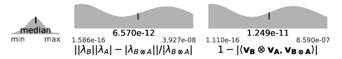
We provide additional MATLAB routines (and precomputed results) making use of Cui, Dai, and Nie (2014); Jaffe, Weiss, and Nadler (2018) as computational verification for theorem 3.3 with randomized symmetric tensors which are small enough to enumerate the entire spectrum of and . As expected, we found no counter examples with random dense symmetric tensors generated with the tensor toolbox Bader and Kolda (2008) where we sample the spectra with Cui et al.’s constrained polynomial optimization Cui, Dai, and Nie (2014) and Jaffe et al’s Newton correction method (and it’s orthogonal variant) Jaffe, Weiss, and Nadler (2018). We report the relative difference between largest magnitude z-eigenvalue found for , , and , and the inner product of the associated eigenvectors in figure 1. This identified no exceptions to our theorem up to computational tolerances.
4 Faster Higher Order Graph Alignment Methods via Kronecker Structure
We show how the tensor Kronecker product results from the previous section allow us to improve the higher-order network alignment algorithm TAME Mohammadi et al. (2017) in two ways. First, Lemma 3.2 is the key to understanding how to use the Kronecker structure to make the iteration from TAME faster when and is low-rank and the number of modes – equivalent to the size of the motif – is not too large. Second, when expanding to larger motifs, such as 9-cliques, we will need to rely on our new simpler algorithm -TAME (§4.3), which is built upon our novel decoupling result, Theorem 3.3.
4.1 Background on higher-order graph alignment
Higher-order graph alignment considers motifs, or small subgraphs, beyond edges Conte et al. (2004); Bayati et al. (2013); Singh, Xu, and Berger (2008) that are matched between a pair of networks. A motif is simply a graph – usually small, like a triangle – and an instance of a motif in a graph is simply an instance of an isomorphic induced subgraph Milo et al. (2002). From any graph we can induce a -regular hypergraph by identifying hyperedges with the presence of motifs with vertices Estrada and Rodríguez-Velázquez (2006); Klymko, Gleich, and Kolda (2014); Benson, Gleich, and Leskovec (2015); Mohammadi et al. (2017). Then the full edge set of the hypergraph involves enumerating all the instances of the motif. This can be computationally demanding to enumerate complicated motifs, but is fast for simple motifs like triangles and small cliques, and random sampling can make the process reasonable for larger cliques Jain and Seshadhri (2020). Analogously to the adjacency matrix, we use an adjacency tensor to denote the presence of these motifs, or equivalently, hyperedges. Formally,
Each permutation of the indices corresponds to a different orientation of the motif . Consequently, the adjacency tensor of a hypergraph is a symmetric, cubical tensor for the motifs we consider.
The higher-order graph alignment problem we consider is defined in terms of a matching between the vertices of two graphs Chertok and Keller (2010); Park, Park, and Hebert (2013); Mohammadi et al. (2017). For a pair of graphs and we characterize a matching between their vertex sets as a matrix.
Definition 4.1 (Matching Matrix).
Let and be two graphs of size and respectively, then we define the matching matrix such that
We suppose we are given a similarity tensor where entries can be indexed using a pair of tuples to represent the vertices of a motif in graph and to represent the vertices of motif from graph . The value indicates the similarity of the motif at indices in graph to the motif at indices in graph . A simple form of higher-order graph alignment problem is to optimize
The goal here is to find high-similarity entries where the vertices involved in the motifs are matched. This subsumes an edge-based alignment framework (such as Feizi et al. (2019)) because could have just been the pair .
We often find it convenient to write this objective as
where we convert the similarity tensor into a tensor indexed with the same order with the operator. This tensor to “operator for ” transformation is something we repeatedly use and write it as
| (6) |
This vec-form makes the eigenvector-heuristic inspiration clear because eigenvectors optimize the generalized Rayleigh quotient .
Many choices for give rise to tensors with Kronecker structure. In TAME Mohammadi et al. (2017), we set to if there is a triangle at both in and in . This idea gives Kronecker structure in . If we denoted the triangles of and in the triangle adjacency tensors and respectively, TAME’s similarity tensor would be . Though simple, this form is informative when given a matching , as
This also gives us a tensor . Again, this framework is highly flexible. For example, the computer vision algorithm HOFASM Park, Park, and Hebert (2013) approximates a similarity tensor between pairs of triplets of a image features with a tensor of the form . For simplicity, we define the following objective function that will guide our subsequent research.
Definition 4.2 (Global Graph Alignment).
Fix graphs and to have and vertices respectively, an prior weight matrix , and a motif with vertices. Let be a -mode similarity tensor where the entry denotes the similarity between the motifs induced by the vertices in graph and in graph . Then we wish to find a matching between the vertices in to the vertices in which optimizes
Equivalently, we let be the -mode “vec-operator” form of , i.e. or . Then the problem is
| (7) |
which makes the tensor-eigenvector inspiration clear (see Sec. 2.2).
The tensor will change depending on what structure we will consider for the higher order matching problem and we may adjust the weightings between the prior matrix and the affinity tensors (a similar edge based framework can be found Berg, Berg, and Malik (2005)). Note that is not required to be symmetric in permutations of the first entries, which are permutations of , but in the problems we consider in this paper, it will be. Likewise for permutations of the last entries for . Note that this means that is a symmetric tensor, although is not even cubical.
4.2 TAME and LowRankTAME
TAME is a spectral method that uses a tensor-eigenvector heuristic to guide an alignment. It arises from the network alignment literature in bioinformatics. The TAME method is a simple instance of the higher-order graph alignment framework (Definition 4.2) where, given two graphs and , we first enumerate triangles (or any motif of interest) in each, to build triangle adjacency tensors and . Then we set . For this choice, we have
| (8) |
This results in the following idealized optimization problem for TAME
| (9) |
Here the value arises because each triangle alignment gives 6 entries in due to symmetry. The weight matrix gives flexibility to bias the alignment towards certain nodes. When no prior matrix is available, we make use of a rank 1 matrix , which gives a uniform bias everywhere.
The heuristic procedure used in TAME is to deploy the SS-HOPM algorithm Kolda and Mayo (2011) to seek a tensor eigenvector, or near tensor eigenvector, of . We show the procedure in Algorithm 1. We present an affine-shift variant of the TAME method that includes the mixing parameter to re-mix in the original iterate whereas TAME Mohammadi et al. (2017) fixed . This choice sometimes helps boost performance a little bit.
Rounding with matching and scoring. At each iteration, we explicitly round the continuous valued and compute a matching using a max-weight matching algorithm. Then the procedure returns the best iterate with the highest downstream objective (triangle alignment, mixture, or some other combination). Returning the full iterate information is helpful for further refinement of the solution using a local search strategy described in §4.4. This max-weight matching step, which is executed at each iteration, becomes expensive after we optimize the linear algebra using the Kronecker theory.
Implicit multiplication. In TAME the authors make use of an implicit operation to compute the iterates of the tensor powers
| (10) |
without forming . This computation still takes work, where nnz is the number of non-zero entries in the sparse tensor. In the case of the uniform bias prior (), the first iterate is rank-1, so we could apply lemma 3.1 to decouple the operation. Because of the shift , however, subsequent iterations will not remain rank 1 as the following observation clarifies.
Our observation. Suppose that is rank 1 and we are dealing with a -mode tensor. Then lemma 3.2 applied to the TAME iteration, states that if is rank then the next iterate has rank at most . This follows from the number of combinations of vectors in the lemma combined with the addition of the rank factors for the previous iterate in the shift. Also can be reduced to for the symmetric case, but for simplicity we use the upper-bound .
While this observation explains a simplistic analysis for the worst case scenario for the rank growth of the iterates, in practice we find it extremely conservative. (See evidence in §5.2.) This means that there is a useful low-rank strategy to employ with our theory. Namely, use Lemma 3.2 to compute the components of the next iterate and then compute an exact low-rank factorization. As long as the rank does not get too big, this will be faster.
An exact low-rank TAME iteration. Let be the low-rank factors of the weight matrix and let be the rank of the initial matrix. The key idea of low-rank TAME, is to compute a rank factorization of the iterate and use lemma 3.2 to compute all the terms in the summation expansion to give us . (This is for triangle tensors.) The low rank terms of next iteration are found by running a rank revealing factorization (such as the SVD or rank-revealing QR) on and concatenated with the low rank terms of the previous iterations and initial iterate (scaled by the appropriate and .) The full procedure is detailed in Algorithm 2.
The dominant terms in the overall runtime of this approach for -node motifs is where RRF is the cost of the rank-revealing factorization. There are many options for the RRF, including randomized and tall-and-skinny approaches. In our codes and the pseudocode we use a rank-revealing method inspired by the R-SVD (which does a QR factorization before an SVD to reduce the work in the SVD) and the structure of our problem. More on the asymptotic runtime of the R-SVD vs SVD can be found in (Golub and van Loan, 2013, Figure 8.6.1). Representative values of the ranks are typically and are much smaller than or (see more discussion in §5.2).
The primary limitation to contracting with low rank components is how much memory explicitly computing the terms requires. When , then building and is preferable because finding the low rank components for the next iteration can be done more efficiently and accurately than a dense . (For accuracy, see §A.1). If then running the original TAME implicit multiplication procedure will be faster (as can be seen in the 7 clique results of figure 9). However when , then the matrices and become wide. In these cases, the low rank structure itself is only beneficial in reducing overall work. Thus, we can simply accumulate the results treat as accumulation parameter and update it with the outer product of the columns of and as we compute them. This can be made more efficient by computing batches of columns, but the best batch size will be system dependent and is a level of tuning we leave to end users.
4.3 -TAME
The inspiration for using SS-HOPM in TAME is that TAME’s objective function (9) is nearby the dominant eigenvector problem for . Given the observation in theorem 3.3 that the dominant eigenvector is built from the dominant eigenvectors of and , this suggests a new heuristic which can be run using only the tensor powers sequences of and independently, rather than combining them as is done in TAME. We then store each of the iterates into a pair of matrices and and use the information in and to derive the matching. There exist many possible ways to derive a matching from the iterates stored in and (see Nassar et al. (2018) for many low-rank ideas). We found that performing a max-weight matching on was the most accurate for downstream alignment tasks in our initial investigation. This is a heuristic choice. Our only ad-hoc justification is that, if these had been matrices, this would have been a set of inner-products among the Krylov basis. We discuss additional useful refinement of and in the next section. We call this method -TAME because it is inspired by our dominant Z-eigenvalue theorem.
Again, we adopted an affine-shift variant of the TAME method that includes an factor to reintroduce the original vector into the solution. This can be set to so that the iterates are exactly those from the SS-HOPM method, but there are cases where helps. In the algorithm, both and can be computed in time proportional to the number of non-zeros of their tensors times the total number of iterations. Like LowRankTAME, the computational bottleneck of this algorithm becomes the matching and refinement steps (see figure 7).
4.4 Matching Refinement
Refining the final matching is a necessary addition when using either TAME, LowRankTAME, and -TAME. For each method, the result is both a low-rank matrix , along with the rank factors , and a maximum weight matching computing on this matrix. In the original TAME method, the matrix was improved by computing a maximum weight bipartite matching and then by looking locally for potential match swaps which montonically increase triangles aligned. Another approach using with a low-rank method is to use the information and matching produced to initialize and guide a more expensive network alignment method, such as Klau’s algorithm Klau (2009), similar to what was done in Nassar et al. (2018).
TAME’s -matching local search refinement TAME’s refines its produced matching by constructing local neighborhoods of nodes and looking for substitutes in its current matchings that increase the number of triangles aligned (or increases the number of edges while maintaining the triangles aligned.) The authors construct a -matching from the matrix returned by TAME (using the 2-approximation algorithm Khan et al. (2016)) and search the found matchings along with neighbor substitutions as local neighborhoods. Each edge in the matching, in order of their edge weight, searches the set of alternative matches
for a possible replacement, and immediately makes changes which improve the alignment. The full procedure is outlined in (Mohammadi et al., 2017, section 4.5, Algo. 4). The original method ascribes weights the edges and triangles using the weights in the iterate returned by TAME, but our method doesn’t weight the triangles or edges when measuring the change in alignment quality. The greedy swapping procedure can be run multiple times, but improvements tend to stop after 5-10 successive sweeps over all matched edges.
A new nearest neighbor local search refinement. The low rank structure of , suggests that an alternative to -matching, for which even the 2-approximation is computationally costly on a large, dense matrix . Rather than -matching, we treat the low-rank structure as an embedding of each vertex where rows of give coordinates for each vertex in graph and rows of give coordinates for each vertex in graph . Then we consider nearby vertices as alternative matches. For this task, a nearest neighbors methodology applies. Each row of embeds , so the rows of which are close to in -norm distance define a natural neighborhood of . This leads us to construct sets of the form
to search for changes to the matchings. Ball-trees are particularly suitable for finding close neighbors of points in low dimensional spaces and are empirically faster than -matching with superior results.
Improving matchings with Klau’s algorithm. Klau’s algorithm Klau (2009) is an edge based graph matching / network alignment method that uses a sequence of maximum weighted matchings to iterate towards a better solution. It can, in some instances, identify optimal solutions of the NP-hard graph matching objective with a corresponding proof of optimality. The algorithm is built from a Lagrangian decomposition of a tight linear program relaxation of the graph matching IQP (a weighted form of Def. 4.2). A full explanation of the algorithm can be found in (Bayati et al., 2013, section 4.3). The primary input for Klau’s method are the graphs , and a weighted bipartite graph between the vertex set of and that restricts and biases the set of possible alignments. The adjacency matrix of this bipartite graph is and is called the link matrix or prior matrix. The method is most effective when has only a few choices for alignments between the graphs.
Thus, we use the results of LowRankTAME or -TAME to build . We include the matched edges within and then expand using the neighborhoods of the matched nodes (much like TAME’s local search). In Nassar et al. (2018), Klau’s method was more accurate when given expanded results of b-matching. Given the low rank structure of our methods, we further expand by including edges in the found matchings with the closest neighbors of in their respective embedding spaces and .
5 Empirical Comparisons in our Network Alignment application
The major demonstration of the new Kronecker product theory is in terms of its impact on network alignment algorithms described in the previous sections. We have implementations of TAME which compute contractions using the original implicit form and new versions using our and existing tensor Kronecker theory. These are all generalized to work with any order motif. We focus on cliques as the motif. We use TuranShadow Jain and Seshadhri (2017) to sample the network for cliques at random. Equivalently, we use cliques to induce a hypergraph where the nodes are the same and the cliques are hyperedges. Our codes are implemented in Julia and are available from https://www.cs.purdue.edu/homes/ccolley/project_pages/TensorKroneckerProducts.html. In this section, we validate the algorithms and show we can achieve similar results with greatly improved runtimes. Some highlights of our results:
-
1.
Iterates of TAME are low rank on real and synthetic data and LowRankTAME computes them an order of magnitude faster for small enough motifs (§5.2).
-
2.
The -TAME vector information can be produced quickly for any size motif.
-
3.
When the -TAME vector information is refined using the nearest neighbor information and Klau’s algorithm, it aligns more triangles and edges than the refined TAME information. Also, it has end to end runtimes 1-2 orders of magnitude faster than the C++ TAME implementation (§5.4).
We use all the same parameters as the original research where they were accessible and will discuss our reasoning for our choices for unlisted parameters. Our experiment environment uses Intel Xeon Platinum 8168 CPUs (@ 2.70GHz) processors with 24 cores, although none of our methods use multicore parallelism. We compare our methods against one another as well as LowRankEigenAlign Nassar et al. (2018). LowRankEigenAlign utilizes low rank structure discovered in the EigenAlign Feizi et al. (2019) algorithm and improves its scalability with minimal changes or even sometimes improvements to accuracy. LowRankEigenAlign has been tested on similar real world and synthetic alignment problems, and its low rank structure makes it a comparable method in terms of memory to -TAME. LowRankEigenAlign also gives a low rank embedding which allows us to refine its results in the manner similar to -TAME and LowRankTAME.
5.1 Data for network alignment experiments
There are two types of data that we use in evaluating the new network alignment algorithms. The first is a subset of the LVGNA Vijayan and Milenković (2017) protein-protein interaction (PPI) graph collection. Each pair of networks in this collection gives an alignment problem. Network statistics are in the supplemental materials (Table 1). Each vertex represents a protein and the edges represent interactions. The networks range in size from 2871 to 16060 vertices and all but the largest networks have fewer triangles than edges.
The second type of data involve synthetic random geometric (RG) graphs. To generate a RG graph, we randomly sample points in the unit square. Then each point adds undirected edges to the nearest neighbors, where is drawn from a log-normal distribution centered at with . We then create a pair of networks to align from this starting reference graph by independently perturbing them from a noise model. The two noise models we consider are (i) a microbiological inspired partial duplication procedure Bhan, Galas, and Dewey (2002); Chung et al. (2003); Hermann and Pfaffelhuber (2014) and (ii) the Erdős-Rényi (ER) noise model from (Feizi et al., 2019, section 3.4). When using the duplication noise mode, we incrementally duplicate 25% new nodes in the network, copying their existing edges with probability . For the ER noise we randomly delete edges with probability and randomly add in edges with probability , where is the density of the network. A few experiments have different choices for these parameters, which will be explicitly noted. We further randomize the permutation of the perturbed network to avoid any influences due to node order in what might happen in the presence of tied values. (Prior work and experience has shown a startlingly strong effect due to biases when this permutation step is not present.) Within each experiment, algorithms are always tested on exactly the same set of networks instead of separate draws from the same distribution.
5.2 Low-rank structure in TAME
For our first set of experiments, we want to show that the iterations from TAME (Algorithm 1) remain low rank when we start with a uniform, or unbiased iterate as the weight matrix: , which is rank 1. We further investigate this behavior on larger motifs. To do this, we report matrix rank using the LowRankTAME algorithm instead of the raw TAME algorithm, which are identical in exact arithmetic (see Aside 5.2).
Aside 1. This choice of exact LowRankTAME vs. TAME to evaluate rank is made both because it is faster to compute but also because preliminary experiments showed that TAME caused the finite precision rank to grow even when the result is mathematically rank 1 (, , by lemma 3.1). This is well-known to happen to finite precision computations, for instance in the power method. Details of this test are in the Supp. A.1.
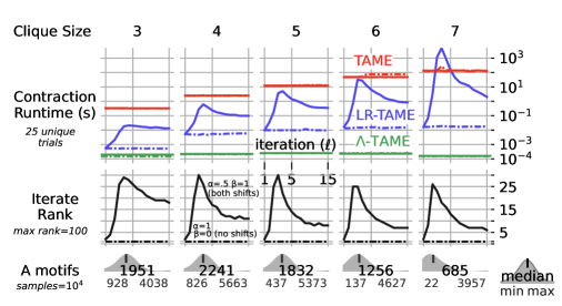
Given either a pair of networks from LVGNA or a synthetic alignment problem, we plot the maximum rank from any iteration on any trial ( running 15 iterations) as determined by the rank function in Julia, as we vary the parameter in the alignment problem. (See Figure 3.) These results, along with trendlines for the maximum rank over multiple repetitions of the synthetic experiments, show that the rank is often below even though the largest networks have 10k vertices.
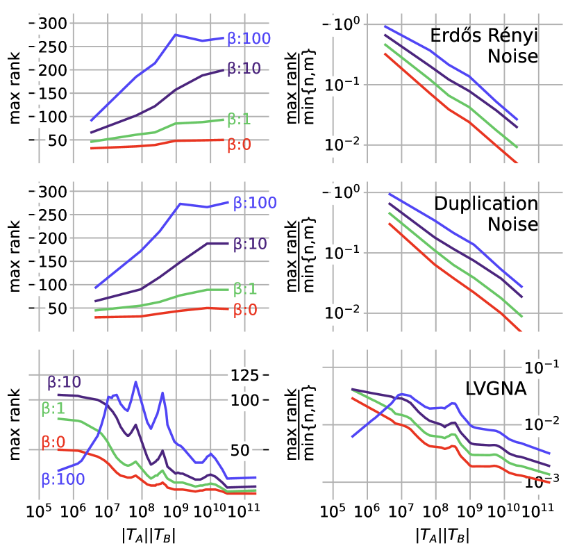
Our rank experiments show the synthetic problems have higher ranks than the LVGNA collection. For the LVGNA collection, large problems tend to have smaller rank, whereas we do see the rank grow with the size of the synthetic problems. For the synthetic problems, we also see that increasing produces higher ranks because these problems incorporate more of the previous iterate via an affine shift. The behavior with for the LVGNA collection is rather different, with many small dips. On further investigation, we found this occurs because is nearly an eigenvalue of these problems. We verified in subsequent experiments that shifting by the estimated eigenvalue gives very small rank, although we do not report these experiments in the interest of space.
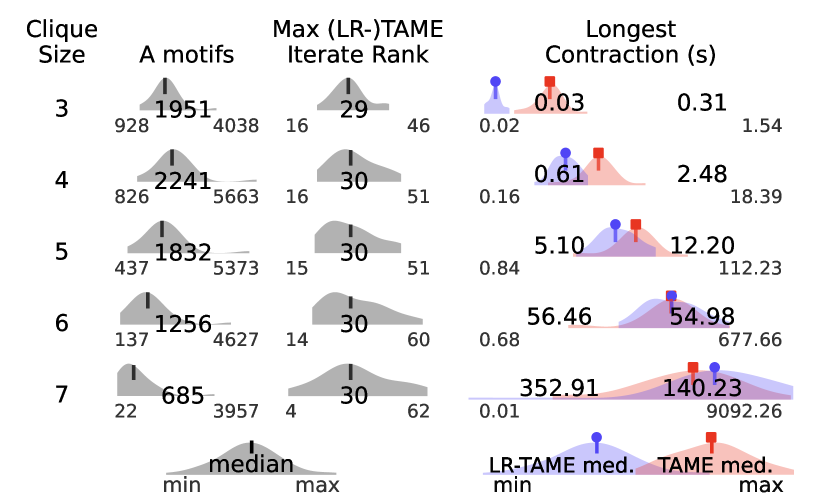
In Figure 3, we investigate rank behavior for larger clique motifs. We see that though the rank of iterates does not change dramatically (second column of density plots), the runtime of TAME and LowRankTAME consistently grows (blue and red density plots in third column), even when the number of motifs within the networks decline (first column of density plots). As the motif size grows, the time spent using the low rank contraction routines approaches the runtime of TAME’s implicit contraction. This becomes salient when memory constraints require a user to use the accumulation form of LowRankTAME, as then even the low rank components are found from a dense matrix , rather than being able to benefit from two R-SVD calls. In summary figure 3 indicates that for small motifs (less than size 6), we can improve the runtime and accuracy using the contraction theory shown in this paper, but those benefits are reduced or even eliminated for problems with larger motifs.
5.3 Alignment Accuracy in Synthetic Networks
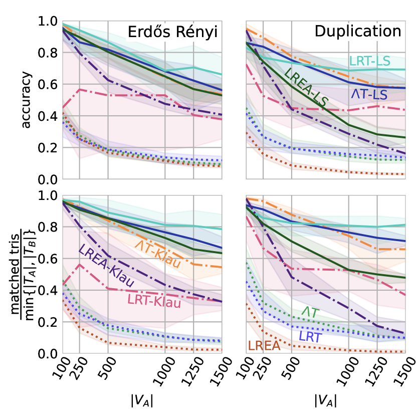
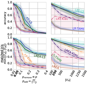
The next set of experiments transitions from runtime to accuracy where we test how well the best low rank results produced by the TAME method, -TAME, and LowRankEigenAlign can be refined by local search and Klau’s algorithm using the -nearest neighbor strategy. We focus on the synthetic problems where there is a single reference graph that is subject to two independent perturbations. The goal is to find the alignment between the vertices of the original reference graph, which we regard as the correct answer. Each combination of methods is compared using the accuracy
and their triangle alignment score (how many triangles they match compared to the maximum possible). We use max iterations , stopping tolerance , and throughout the experiments – except in figures where is varied. We focus on our experiments which vary the size of alignment problems. Additional parameters of our noise models are studied in the supplement S.4.2.
The first set of experiments focuses on triangles. These experiments show that all three methods require refinement to get practical results, especially as the problems get larger. (figure 5). These experiments show that LowRankTAME with the local search strategy -NN had the best performance for the largest problems, although -TAME with Klau’s refinement was slightly better at intermediate sized problems for the duplication noise model.
We can also see that triangles matched is a good proxy for the accuracy of the matchings, although depending on the noise models, there may be deviations.
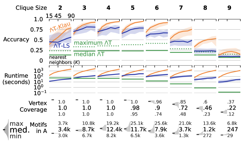
Moreover, with the -NN refinement and -TAME’s scalability, we can get fast accurate matchings for not only large networks, but also increasingly larger clique sizes (figure 5). Accuracy remains high when the vertex coverage, the fraction of the total vertex set involved in motifs, remains high. In contrast to the results with LowRankTAME (figure 3), using -TAME has a practical runtime for large cliques. Klau’s algorithm can offer an additional benefit if a longer runtime can be tolerated.
We also find that our default choice of gets good performance. Increasing can improve accuracy slightly, but Klau’s algorithm runtime is more sensitive to the sparsity of the input link matrix. Local search remains very fast with a modest increase in runtime as the local search neighborhoods are expanded. It’s unsurprising to see that Klau’s algorithm matches the fewest motifs given the objective function is focused on aligning edges between networks.
5.4 Biological Networks
We now turn our attention to considering the performance within real world networks from biology. We report the end to end runtime, triangles matched, and edges matched of each refined method relative to TAME, over pairs of alignment problems from LVGNA in figure 7 (see §S.4.3 for non-comparative results). We use max iterations , stopping tolerance , and nearest neighbors for refinement. We see that -TAME refined with local search aligns more triangles and edges and runs much faster than the original TAME. All methods tested align more edges than TAME, though improving with local search was much more likely to increase triangles matched. Methods using Klau’s algorithm or LowRankEigenAlign increased the number of edges aligned, but aligned fewer triangles. This was observed in the synthetic results in 5 and is unsurprising given each method’s focus on edges.
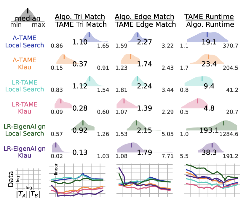
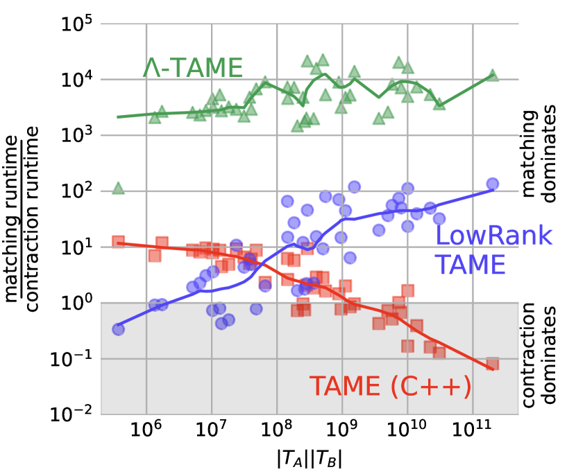
Returning to timing, we compare the fraction of time spent in the matching vs. matrix / tensor operations in figure 7. We can see that the Kronecker theory here makes the time to compute the contractions fast enough to change the primary bottleneck of the algorithm when using triangle adjacency tensors. Put simply, -TAME always spends more time on the bipartite matching and refinement and LowRankTAME spends more time there on the biggest problems. A primary reason for why -TAME and LowRankTAME spend so much time computing the matchings is that we cannot take advantage of the low rank structure. We compute the maximum matching using the Primal-Dual algorithm Dantzig, Ford Jr, and Fulkerson (1956), which must touch each entry of at least once, making it more efficient to form explicitly at the beginning of the algorithm. This suggests potential future research for new algorithms which can properly make use of the low rank structure, while still computing a maximum weighted matching.
6 Discussion
The major focus of our paper is on demonstrating how the theory on tensor Kronecker products in §3 enables us to accelerate the graph matching algorithm TAME (§4): (i) by making the same algorithm faster with LowRankTAME, (ii) by giving a new, faster algorithm (-TAME), and (iii) by providing new augmentations of TAME’s local search and Klau’s algorithm which can make use of the low rank structure within the iterates.
One interesting theory question we have not pursued is the opposite of the example from the introduction that shows diagonal tensors have eigenvectors that are not a Kronecker product. Put concretely, is there a class of tensors where no new eigenvectors emerge after taking a Kronecker product?
On the application side, the new method -TAME’s runtime is heavily dominated by the rounding and refinement procedures, as seen in figure 7. Our implementation uses the primal-dual algorithm which is an effective solution when is explicitly realized as a dense matrix. New matching methods which compute the maximum matching of while only using and would be useful to improve scalability (even if only an approximation). For large enough problems, there are also low-rank matching heuristics from Nassar et al. (2018) to consider for additional scalability, although the results from these methods were noticeably worse for our case compared with using the exact max-weight matching.
Low-rank structure offers a few benefits even beyond the reduced runtime. First, we are able to explicitly store a large number of TAME iterates as low-rank factorizations. Sending data is much faster to send between cores, which may offer footholds in known parallel matching challenges Sathe, Schenk, and Burkhart (2012); Bertsekas and Castañon (1991). Applying theorem 3.3 recursively suggests an immediate algorithm for multi-network alignments. Each network’s embeddings can be computed independently in a fashion similar to that used in Nassar et al. (2021). Furthermore, we also see opportunities to incorporate multiple network motifs within adjacency tensors. Smaller motifs could be encoded into in the off diagonal components (see Aside 6). Motif complexes could be encoded into the off diagonal components in a way that wouldn’t change contraction or eigenvector definitions.
Aside 2. Tensors can have more than one “diagonal” by grouping non-zeros by the multiplicity of their indices. In a triangle adjacency tensor the non-zeros are of the form for distinct vertices and the traditional diagonal is comprised of the indices . A third order tensor also has entries which only have two unique vertices, and the presence of an edge could be marked in an entry of the form or . These off diagonals are referred to as -multiplicity tensors in (Yan et al., 2015, Def. 2).
The fashion in which we construct the embeddings is also closely related to various graph kernels Vishwanathan et al. (2010); Kriege, Johansson, and Morris (2020) including the random walk kernel on a direct product graph. Graph kernels have long been used to align small chemicographs (graphs that represent small chemical molecules). In this case, we are able to generate a direct factorization of a graph kernel between vertices of two graphs into a product of features on each graph. This is a common paradigm Vishwanathan et al. (2010) involving matrix Kronecker products—although we are unaware of any research on this for higher order analogues of the graph kernels involving tensor Kronecker products that would be needed for our perspective. When viewed in this light, our research has the potential to open new directions in this space in terms of efficient graph kernels on hypergraphs.
In summary, our theory and experiments show how the computational demands of methods with tensor Kronecker products may be reduced by orders of magnitude with no change in quality, or accelerated even further with useful approximate results. We are excited about the future opportunities with tensor Kronecker products due to the widespread use of matrix Kronecker products, and suspect that these theorems, or alternative generalizations that use specific structure in novel problems, will be a key element in this future research.
Acknowledgments
We thank O. Eldaghar for the fruitful conversations when designing our figures and C. Cui for discussions on the code from Cui, Dai, and Nie (2014).
Appendix A Additional information
A.1 TAME rank-1 Singular Value Experiments
These experiments explain why we use the exact LowRankTAME iteration instead of the original TAME iteration to study rank when using triangle adjacency tensors. They show TAME produces iterates that would be detected as at least rank-2 even when the answer is provably rank-1, whereas LowRankTAME does not. Figure 8 plots the maximum second largest normalized singular values of , , of all 15 iterations for TAME and LowRankTAME of the rank 1 iteration case for the LVGNA and our synthetic alignments. Hollow points are values small enough to be considered zero (and hence, would be rank-1), and filled points are large enough to be measured as non-zero (and hence, would be rank-2). The LVGNA experiments align all pairs of distinct networks. The synthetic experiments are measured over 50 trials using random geometric graphs. Seeded networks are perturbed by both ER and Duplication noise models using default parameters.
A.2 PPI Graph Statistics
We use networks from the LVGNA project Meng, Striegel, and Milenković (2016), the statistics of which (unique edges and triangles) are in Table 1. These networks have been aligned with a variety of contemporary methods in Vijayan and Milenković (2017); Meng, Striegel, and Milenković (2016); Nassar et al. (2018), to make our results comparable with prior research. We remove any directional edges from the network before the enumerating triangles. As our methods are focused on triangle motifs, we only use networks with more than 150 triangles. We also include the largest sampled z-eigenvalue found, which – like the standard power method – is related to the behavior of the methods with shifts in §5.2.
| Graph Name | Vertices | Edges | Triangles | Sampled |
|---|---|---|---|---|
| worm_Y2H1 | 2871 | 5194 | 536 | 10.076 |
| worm_PHY1 | 3003 | 5501 | 692 | 12.664 |
| fly_Y2H1 | 7094 | 23356 | 2501 | 21.207 |
| yeast_Y2H1 | 3427 | 11348 | 9503 | 56.680 |
| human_Y2H1 | 9996 | 39984 | 15177 | 72.919 |
| human_PHY2 | 8283 | 19697 | 19190 | 50.872 |
| yeast_PHY2 | 3768 | 13654 | 26295 | 94.564 |
| fly_PHY1 | 7885 | 36271 | 58216 | 217.541 |
| yeast_PHY1 | 6168 | 82368 | 381812 | 454.921 |
| human_PHY1 | 16060 | 157649 | 525238 | 488.136 |
References
- Akoglu, McGlohon, and Faloutsos (2008) L. Akoglu, M. McGlohon, and C. Faloutsos. RTM: Laws and a recursive generator for weighted time-evolving graphs. In Proceedings of ICDM, pp. 701–706. 2008.
- Bader and Kolda (2008) B. W. Bader and T. G. Kolda. Efficient matlab computations with sparse and factored tensors. SIAM Journal on Scientific Computing, 30 (1), pp. 205–231, 2008.
- Batselier and Wong (2017) K. Batselier and N. Wong. A constructive arbitrary-degree kronecker product decomposition of tensors. Numerical Linear Algebra with Applications, 24 (5), p. e2097, 2017.
- Bayati et al. (2013) M. Bayati, D. F. Gleich, A. Saberi, and Y. Wang. Message-passing algorithms for sparse network alignment. ACM Trans. Knowl. Discov. Data, 7 (1), pp. 3:1–3:31, 2013. doi:10.1145/2435209.2435212.
- Bazaraa and Kirca (1983) M. Bazaraa and O. Kirca. A branch-and-bound-based heuristic for solving the quadratic assignment problem. Naval research logistics quarterly, 30 (2), pp. 287–304, 1983.
- Benson and Gleich (2019) A. R. Benson and D. F. Gleich. Computing tensor z-eigenvectors with dynamical systems. SIAM Journal on Matrix Analysis and Applications, 40 (4), pp. 1311–1324, 2019.
- Benson, Gleich, and Leskovec (2015) A. R. Benson, D. F. Gleich, and J. Leskovec. Tensor spectral clustering for partitioning higher-order network structures. In Proceedings of SDM, pp. 118–126. 2015. doi:10.1137/1.9781611974010.14.
- Berg, Berg, and Malik (2005) A. C. Berg, T. L. Berg, and J. Malik. Shape matching and object recognition using low distortion correspondences. In Proceedings of CVPR, pp. 26–33. 2005.
- Bertsekas and Castañon (1991) D. P. Bertsekas and D. A. Castañon. Parallel synchronous and asynchronous implementations of the auction algorithm. Parallel Comput., 17 (6-7), pp. 707–732, 1991. doi:10.1016/S0167-8191(05)80062-6.
- Bhan, Galas, and Dewey (2002) A. Bhan, D. J. Galas, and T. G. Dewey. A duplication growth model of gene expression networks. Bioinformatics, 18 (11), pp. 1486–1493, 2002.
- Blondel et al. (2004) V. D. Blondel, A. Gajardo, M. Heymans, P. Senellart, and P. Van Dooren. A measure of similarity between graph vertices: Applications to synonym extraction and web searching. SIAM review, 46 (4), pp. 647–666, 2004.
- Burkard, Dell’Amico, and Martello (2012) R. Burkard, M. Dell’Amico, and S. Martello. Assignment Problems, SIAM, revised edition, 2012. doi:10.1137/1.9781611972238.
- Cartwright and Sturmfels (2013) D. Cartwright and B. Sturmfels. The number of eigenvalues of a tensor. Linear Algebra Appl., 438 (2), pp. 942–952, 2013.
- Chertok and Keller (2010) M. Chertok and Y. Keller. Efficient high order matching. IEEE Trans. Pattern Anal. Mach. Intell., 32 (12), pp. 2205–2215, 2010.
- Chung et al. (2003) F. Chung, L. Lu, T. G. Dewey, and D. J. Galas. Duplication models for biological networks. Journal of computational biology, 10 (5), pp. 677–687, 2003.
- Conte et al. (2004) D. Conte, P. P. Foggia, C. Sansone, and M. Vento. Thirty years of graph matching in pattern recognition. Intern. J. Pattern. Recognit. Artif. Intell., 18 (3), pp. 265–298, 2004. doi:10.1142/S0218001404003228.
- Cui, Dai, and Nie (2014) C.-F. Cui, Y.-H. Dai, and J. Nie. All real eigenvalues of symmetric tensors. SIAM Journal on Matrix Analysis and Applications, 35 (4), pp. 1582–1601, 2014.
- Dantzig, Ford Jr, and Fulkerson (1956) G. B. Dantzig, L. R. Ford Jr, and D. R. Fulkerson. A primal–dual algorithm. Technical report, RAND CORP SANTA MONICA CA, 1956.
- De Lathauwer et al. (1995) L. De Lathauwer, P. Comon, B. De Moor, and J. Vandewalle. Higher-order power method. Nonlinear Theory and its Applications, NOLTA’95, 1, pp. 91–96, 1995.
- Eikmeier, Ramani, and Gleich (2018) N. Eikmeier, A. S. Ramani, and D. F. Gleich. The hyperkron graph model for higher-order features. In Proceedings of the International Conference on Data Mining (ICDM), pp. 941–946. 2018. doi:10.1109/ICDM.2018.00115.
- Estrada and Rodríguez-Velázquez (2006) E. Estrada and J. A. Rodríguez-Velázquez. Subgraph centrality and clustering in complex hyper-networks. Physica A: Statistical Mechanics and its Applications, 364, pp. 581–594, 2006.
- Feizi et al. (2019) S. Feizi, G. Quon, M. Mendoza, M. Medard, M. Kellis, and A. Jadbabaie. Spectral alignment of graphs. IEEE Transactions on Network Science and Engineering, 2019.
- Golub and van Loan (2013) G. H. Golub and C. van Loan. Matrix Computations, Johns Hopkins University Press, 2013.
- Hermann and Pfaffelhuber (2014) F. Hermann and P. Pfaffelhuber. Large-scale behavior of the partial duplication random graph. arXiv preprint arXiv:1408.0904, 2014.
- Jaffe, Weiss, and Nadler (2018) A. Jaffe, R. Weiss, and B. Nadler. Newton correction methods for computing real eigenpairs of symmetric tensors. SIAM Journal on Matrix Analysis and Applications, 39 (3), pp. 1071–1094, 2018.
- Jain and Seshadhri (2017) S. Jain and C. Seshadhri. A fast and provable method for estimating clique counts using turán’s theorem. In Proceedings of the 26th international conference on world wide web, pp. 441–449. 2017.
- Jain and Seshadhri (2020) ———. The power of pivoting for exact clique counting. In Proceedings of WSDM, pp. 268–276. 2020.
- Khan et al. (2016) A. Khan, A. Pothen, M. Mostofa Ali Patwary, N. R. Satish, N. Sundaram, F. Manne, M. Halappanavar, and P. Dubey. Efficient approximation algorithms for weighted b-matching. SIAM Journal on Scientific Computing, 38 (5), pp. S593–S619, 2016.
- Klau (2009) G. W. Klau. A new graph-based method for pairwise global network alignment. BMC Bioinform., 10 (1), p. S59, 2009.
- Klymko, Gleich, and Kolda (2014) C. Klymko, D. Gleich, and T. G. Kolda. Using triangles to improve community detection in directed networks. arXiv preprint arXiv:1404.5874, 2014.
- Kolda and Mayo (2011) T. G. Kolda and J. R. Mayo. Shifted power method for computing tensor eigenpairs. SIAM Journal on Matrix Analysis and Applications, 32 (4), pp. 1095–1124, 2011.
- Kolda and Mayo (2014) ———. An adaptive shifted power method for computing generalized tensor eigenpairs. SIAM Journal on Matrix Analysis and Applications, 35 (4), pp. 1563–1581, 2014.
- Kollias, Mohammadi, and Grama (2011) G. Kollias, S. Mohammadi, and A. Grama. Network similarity decomposition (NSD): A fast and scalable approach to network alignment. IEEE Trans. Knowl. Data Eng., 24 (12), pp. 2232–2243, 2011.
- Koopmans and Beckmann (1957) T. C. Koopmans and M. Beckmann. Assignment problems and the location of economic activities. Econometrica: journal of the Econometric Society, pp. 53–76, 1957.
- Kriege, Johansson, and Morris (2020) N. M. Kriege, F. D. Johansson, and C. Morris. A survey on graph kernels. Applied Network Science, 5 (1), 2020. doi:10.1007/s41109-019-0195-3.
- Lawler (1963) E. L. Lawler. The quadratic assignment problem. Management science, 9 (4), pp. 586–599, 1963.
- Lim (2005) L.-H. Lim. Singular values and eigenvalues of tensors: a variational approach. In 1st Intl. Workshop on Computational Advances in Multi-Sensor Adaptive Processing, pp. 129–132. 2005.
- Malod-Dognin and Pržulj (2015) N. Malod-Dognin and N. Pržulj. L-graal: Lagrangian graphlet-based network aligner. Bioinformatics, 31 (13), pp. 2182–2189, 2015.
- Meng, Striegel, and Milenković (2016) L. Meng, A. Striegel, and T. Milenković. Local versus global biological network alignment. Bioinformatics, 32 (20), pp. 3155–3164, 2016.
- Milo et al. (2002) R. Milo, S. Shen-Orr, S. Itzkovitz, N. Kashtan, D. Chklovskii, and U. Alon. Network motifs: simple building blocks of complex networks. Science, 298 (5594), pp. 824–827, 2002.
- Mohammadi et al. (2017) S. Mohammadi, D. F. Gleich, T. G. Kolda, and A. Grama. Triangular alignment TAME: A tensor-based approach for higher-order network alignment. IEEE/ACM Trans. Comput. Biol. Bioinform., 14 (6), pp. 1446–1458, 2017.
- Nassar et al. (2021) H. Nassar, G. Kollias, A. Grama, and D. F. Gleich. Scalable algorithms for multiple network alignment. SIAM J. Scientific Computing, 43 (5), pp. S592–S611, 2021. doi:10.1137/20m1345876.
- Nassar et al. (2018) H. Nassar, N. Veldt, S. Mohammadi, A. Grama, and D. F. Gleich. Low rank spectral network alignment. In Proceedings of the 2018 World Wide Web Conference, pp. 619–628. 2018.
- Park, Park, and Hebert (2013) S. Park, S.-K. Park, and M. Hebert. Fast and scalable approximate spectral matching for higher order graph matching. IEEE Trans. Pattern Anal. Mach. Intell., 36 (3), pp. 479–492, 2013.
- Patro and Kingsford (2012) R. Patro and C. Kingsford. Global network alignment using multiscale spectral signatures. Bioinformatics, 28 (23), pp. 3105–3114, 2012.
- Phan et al. (2012) A. H. Phan, A. Cichocki, P. Tichavskỳ, D. P. Mandic, and K. Matsuoka. On revealing replicating structures in multiway data: A novel tensor decomposition approach. In Proceedings of LVA/ICA, pp. 297–305. 2012.
- Phan et al. (2013) A. H. Phan, A. Cichocki, P. Tichavskỳ, R. Zdunek, and S. Lehky. From basis components to complex structural patterns. In 2013 IEEE International Conference on Acoustics, Speech and Signal Processing, pp. 3228–3232. 2013.
- Qi (2005) L. Qi. Eigenvalues of a real supersymmetric tensor. Journal of Symbolic Computation, 40 (6), pp. 1302–1324, 2005.
- Qi and Luo (2017) L. Qi and Z. Luo. Tensor analysis: spectral theory and special tensors, Siam, 2017.
- Qi (2018) Y. Qi. A very brief introduction to nonnegative tensors from the geometric viewpoint. Mathematics, 6 (11), p. 230, 2018.
- Ragnarsson-Torbergsen (2012) S. Ragnarsson-Torbergsen. Structured tensor computations: Blocking, symmetries and kronecker factorizations. 2012.
- Sathe, Schenk, and Burkhart (2012) M. Sathe, O. Schenk, and H. Burkhart. An auction-based weighted matching implementation on massively parallel architectures. Parallel Computing, 38 (12), pp. 595–614, 2012. doi:10.1016/j.parco.2012.09.001.
- Shao (2013) J.-Y. Shao. A general product of tensors with applications. Linear Algebra and its applications, 439 (8), pp. 2350–2366, 2013.
- Shen et al. (2018) T. Shen, Z. Zhang, Z. Chen, D. Gu, S. Liang, Y. Xu, R. Li, Y. Wei, Z. Liu, Y. Yi, et al. A genome-scale metabolic network alignment method within a hypergraph-based framework using a rotational tensor-vector product. Scientific reports, 8 (1), pp. 1–16, 2018.
- Singh, Xu, and Berger (2008) R. Singh, J. Xu, and B. Berger. Global alignment of multiple protein interaction networks with application to functional orthology detection. Proc. Natl. Acad. Sci. U.S.A., 105 (35), pp. 12763–12768, 2008.
- Stark et al. (2006) C. Stark, B.-J. Breitkreutz, T. Reguly, L. Boucher, A. Breitkreutz, and M. Tyers. Biogrid: a general repository for interaction datasets. Nucleic acids research, 34 (suppl_1), pp. D535–D539, 2006.
- Sun et al. (2016) L. Sun, B. Zheng, C. Bu, and Y. Wei. Moore–penrose inverse of tensors via einstein product. Linear and Multilinear Algebra, 64 (4), pp. 686–698, 2016.
- Sun, Chen, and So (2018) W. Sun, Y. Chen, and H. C. So. Tensor completion using kronecker rank-1 tensor train with application to visual data inpainting. IEEE Access, 6, pp. 47804–47814, 2018.
- Vijayan and Milenković (2017) V. Vijayan and T. Milenković. Multiple network alignment via multimagna++. IEEE/ACM Trans. Comput. Biol. Bioinform., 15 (5), pp. 1669–1682, 2017.
- Vishwanathan et al. (2010) S. V. N. Vishwanathan, N. N. Schraudolph, R. Kondor, and K. M. Borgwardt. Graph kernels. The Journal of Machine Learning Research, 11, pp. 1201–1242, 2010.
- Yan et al. (2015) J. Yan, C. Zhang, H. Zha, W. Liu, X. Yang, and S. M. Chu. Discrete hyper-graph matching. In Proceedings of the IEEE conference on computer vision and pattern recognition, pp. 1520–1528. 2015.
- Zass and Shashua (2008) R. Zass and A. Shashua. Probabilistic graph and hypergraph matching. In Proceedings of CVPR, pp. 1–8. 2008.
- Zhang, Ling, and Qi (2012) X. Zhang, C. Ling, and L. Qi. The best rank-1 approximation of a symmetric tensor and related spherical optimization problems. SIAM J. Matrix Anal. Appl., 33 (3), pp. 806–821, 2012.
Supplemental Materials
In our supplement we include proofs to lemmas 3.1 & 3.2 in S.3 and additional experiments to provide more context for our discussed results in section 5. Our figures include:
-
1.
a full plot of the iterate runtimes and ranks of the experiments in figure 3,
-
2.
additional experiments for all the parameters in our synthetic alignment noise models put alongside our scaling experiments in figure 5, and
-
3.
the full breakdown of the runtimes and triangle match scores of the LVGNA alignment experiments, with additional results from other comparable alignment algorithms.
S.3 Proofs
Here we include our own proofs of lemmas 3.1 & 3.2. The rank-1 tensor vector contraction lemma is proved inductively whereas our other proof is a more standard algebraic proof. We repeat the lemma statements for readability.
S.3.1 Rank 1 contraction
Lemma S.1.
Given two -mode, cubical tensors and of dimension and , respectively, and the rank 1 matrix , then for ,
| (11) |
Proof S.2.
First note that for any symmetric tensor , we have in our notation for any . Our proof simply uses induction. The base case is . Here, we split the multi-index (for ) into its first component and tail , and do the same for the for . Then
The remainder of the argument is as follows. Assume the result holds for up to some value of , then we can show it holds for via
Note that and are both symmetric, so we can apply the previous result (or the inductive hypothesis). Inductively, now, we have and thus we are done using our initial note.
S.3.2 Rank r contraction
Lemma S.3.
Given two -mode, cubical tensors and of dimension and , respectively, and the matrix with the rank decomposition , then
where is the identity matrix.
Proof S.4.
We show this directly on each element, starting with the first line. Let and . Then
This gets us the second line after we convert to the Kronecker product. To get the last line, we can convert the summation over into a double summation multiplied by an indicator. Essentially, we use . Note that because we have the matrix satisfies . Then
This final result is then just the element of .
S.4 Further Experiments and Additional Results
S.4.1 Maximum Rank
Here we show a breakdown of the runtime and ranks of each of the TAME iterates used for our results in figure 3. We’re able to see that the rank behavior peaks at the earlier iterates of the method and slowly converge to a lower rank iterate (when using both shifts). This is notable as in the original TAME work, the authors observed that the highest quality alignments occurred within the first few iterations Mohammadi et al. (2017, section 5.6). In our experiments we didn’t find that iteration rank was a better proxy for alignment accuracy than triangles align in synthetic experiments.
S.4.2 Random Graph Models
In figure 5 we presented out synthetic alignment results as the reference network’s size was varied, without discussion of our perturbation model’s parameters. Here we include experiments where we vary the remaining modes for Erdős-Rényi and the partial duplication perturbation models. The Erdős-Rényi model from Feizi et al. (2019) removes (and adds) edges as a function of . The partial duplication model randomly duplicates an existing node and uniformly retains each edge with probability . We additionally may vary how long we run the procedure to control how many more vertices are introduced. Our full results are reported in figure 10 along side the original network size experiments for easier comparison.
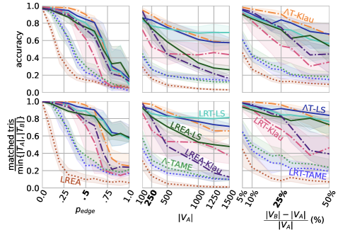
Overall we see similar performance to the size scaling experiments for the other modes, though refined LowRankEigenAlign does better for the additional parameters in the duplication noise models. A notable difference from just the size scaled experiments is that for the and parameters of each noise model, the triangle match rate is much higher than the accuracy. Though the relative performance between the methods is still maintained, this seems to detract a little from it’s role as proxy for accuracy. However this is reasonable given that for the inflation only occurs for the largest amounts of noise used. For the duplication noise, the largest values of is 100% which means that all new duplicated nodes are isomorphic to their original nodes. When permuted, it’s unreasonable to expect an unsupervised algorithm to be able to determine between the original and duplicated node. An analogous problem will occur for the largest values of . Removing and adding in 40% of the potential edges in a network is an extreme perturbation.
S.4.3 LVGNA Alignments
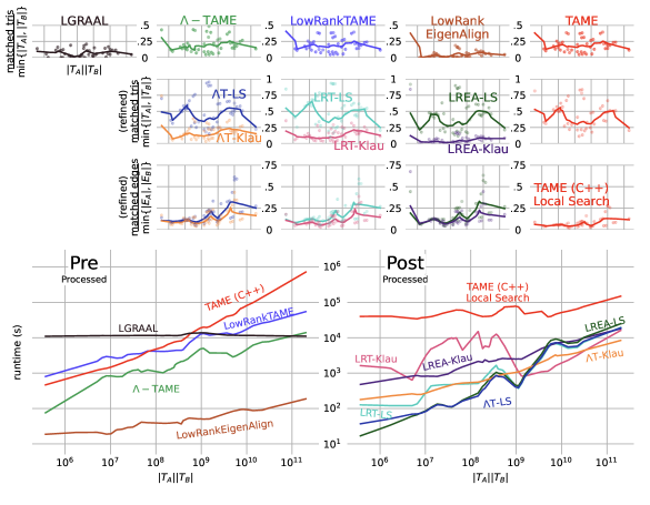
Here we include the full results of the alignment algorithms tested on the LVGNA networks, instead of the relative performance of each algorithm compared to TAME (reported in figure 7). These results show that LowRankTAME is roughly an order of magnitude faster than the implementation of TAME in C++ from Mohammadi et al. (2017) for the largest experiments. -TAME is about two orders of magnitude faster. Given what we see in the bottlenecks demonstrated in figure 7 we can attribute the growth in runtime to growing cost of solving for the maximum weighted matchings instead of the tensor operations. In addition to the previously discussed methods, we also include results using LGRAAL Malod-Dognin and Pržulj (2015). L-GRAAL computes graphlet degrees to guide alignments (similar to other GRAAL methods) and uses Lagrangian relaxations to seed and extend its matchings. L-GRAAL was one of the higher quality, but longer running algorithms in the original TAME paper (Mohammadi et al., 2017, Figure 1,2). We did not find that LGRAAL aligned a sufficient amount of triangles (this is likely due to the objective function focusing on aligning edges). Additionally LGRAAL doesn’t provide an output that we can refine like we can for LowRankEigenAlign or the TAME methods. We include it’s runtime for an additional comparison point to our methods. Its relatively constant runtime is due to the method consistently hitting it’s maximum runtime limit before converging to a solution. We see that LowRankEigenAlign is the fastest method, and when refined provides more edges aligned, but the triangles aligned are not as competitive as the refined LowRankTAME or -TAME embeddings (as was seen in figure 7). We also see that with the exception of the largest alignment problems, the refining runtime is eclipsed by the runtime of the TAME methods. LowRankEigenAlign was the only method to be faster than the refinement. It should also be noted that though the LowRankTAME and TAME triangle matching rates look identical, there are small differences which amount due how ties are broken in the rounding procedures of LowRankTAME and TAME. Edges in TAME’s C++ primal dual implementation are traversed using a row major formatting, whereas our julia implementation uses a column major formatting.