A convergent structure-preserving finite-volume scheme for the Shigesada-Kawasaki-Teramoto population system

Abstract.

An implicit Euler finite-volume scheme for an $n$-species population cross-diffusion system of Shigesada–Kawasaki–Teramoto-type in a bounded domain with no-flux boundary conditions is proposed and analyzed. The scheme preserves the formal gradient-flow or entropy structure and preserves the nonnegativity of the population densities. The key idea is to consider a suitable mean of the mobilities in such a way that a discrete chain rule is fulfilled and a discrete analog of the entropy inequality holds. The existence of finite-volume solutions, the convergence of the scheme, and the large-time asymptotics to the constant steady state are proven. Furthermore, numerical experiments in one and two space dimensiona for two and three species are presented. The results are valid for a more general class of cross-diffusion systems satisfying some structural conditions.

1. Introduction

The population model of Shigesada, Kawasaki, and Teramoto (SKT) describes the segregation of two competing species [32]. It consists of quasilinear parabolic equations for the population densities with a generally nonsymmetric and not positive semidefinite diffusion matrix. To overcome the lack of positive definiteness, it was suggested in [11, 20] to use so-called entropy variables that yield a transformed diffusion system with a positive semidefinite diffusion matrix. In particular, the SKT cross-diffusion system of [32] has a formal gradient-flow or entropy structure. This approach can be generalized to an arbitrary number of species [13]. It is important to design a general easy-to-implement numerical scheme that preserves this structure and that can be proven to be convergent. Previous works like [2, 3, 33] propose numerical approximations that satisfy some of these properties but not all of them. In this paper, we suggest a finite-volume scheme for $n$-species SKT-type population systems, preserving the entropy structure and the nonnegativity of densities and conserving the mass (in the absence of source terms). In fact, our results are even valid for a more general class of cross-diffusion systems satisfying some structural conditions.

More precisely, we consider the cross-diffusion system

(1) $$\partial_{t}u_{i}-\operatorname{div}\bigg{(}\sum_{j=1}^{n}A_{ij}(u)\nabla u_{j}\bigg{)}=f_{i}(u)\quad\mbox{in }\Omega,\ t>0,\ i=1,\ldots,n,$$

where $\Omega\subset{\mathbb{R}}^{d}$ ($d\geq 1$) is a bounded domain, $u=(u_{1},\ldots,u_{n})$ is the vector of population densities, with the diffusion coefficients

(2) $$A_{ij}(u)=\delta_{ij}\bigg{(}a_{i0}+\sum_{k=1}^{n}a_{ik}u_{k}\bigg{)}+a_{ij}u_{i},\quad i,j=1,\ldots,n,$$

and the Lotka–Volterra source terms,

(3) $$f_{i}(u)=u_{i}\bigg{(}b_{i0}-\sum_{j=1}^{n}b_{ij}u_{j}\bigg{)},\quad i=1,\ldots,n,$$

where we assume that $a_{ii}>0$, $b_{ii}>0$ for $i=1,\ldots,n$ and $a_{ij}\geq 0$ and $b_{ij}\geq 0$ for $i\neq j$. We prescribe no-flux boundary and initial conditions:

(4) $$\sum_{j=1}^{n}A_{ij}(u)\nabla u_{j}\cdot\nu=0\quad\mbox{on }\partial\Omega,\ t>0,\quad u_{i}(0)=u_{i}^{0}\quad\mbox{in }\Omega,\quad i=1,\ldots,n,$$

where $\nu$ denotes the exterior unit normal vector to $\partial\Omega$. When $n=2$, we recover the SKT system of [32] without environmental potentials. Our analysis also works when we include the corresponding drift terms (see Section 8.4).

Let $h:[0,\infty)^{n}\to[0,\infty)$ be a convex function and set $H[u]=\int_{\Omega}h(u)dx$. The entropy inequality is derived, for suitable source terms, by choosing $h^{\prime}(u)$ formally as a test function in the weak formulation of (1), leading to

(5) $$\frac{dH}{dt}+\int_{\Omega}\nabla u:h^{\prime\prime}(u)A(u)\nabla udx\leq C(T),\quad 0<t<T,$$

where $h^{\prime\prime}(u)$ is the Hessian of $h$, “:” is the Frobenius matrix product, and $C(T)>0$ comes from the source terms. We call $H$ an entropy and $h$ an entropy density if $h^{\prime\prime}(u)A(u)$ is positive (semi-) definite. This typically provides gradient estimates and moreover, if $C(T)=0$, then $H$ is a Lyapunov functional along the solutions to (1).

In the case of the $n$-species SKT model, the entropy density is given by

(6) $$h(u)=\sum_{i=1}^{n}\pi_{i}\big{(}u_{i}(\log u_{i}-1)+1\big{)},\quad u\in[0,\infty)^{n},$$

where the numbers $\pi_{i}>0$ are assumed to satisfy $\pi_{i}a_{ij}=\pi_{j}a_{ji}$ for $i\neq j$. This can be recognized as the detailed-balance condition for the time-continuous Markov chain associated to $(a_{ij})$, and the vector $(\pi_{i})$ is the corresponding invariant measure [13]. It turns out that $\nabla u:h^{\prime\prime}(u)A(u)\nabla u$ is bounded from below by $\sum_{i=1}^{n}a_{ii}|\nabla u_{i}|^{2}$, which yields $H^{1}(\Omega)$ estimates. Moreover, it can be shown that the solutions $u_{i}$ are nonnegative and the mass $\int_{\Omega}u_{i}(t)dx$ is constant in time if $f_{i}=0$. Our aim is to preserve this structure on the discrete level.

In the literature, there are already various numerical schemes for the SKT model. Up to our knowledge, the first numerical simulations, based on a finite-difference scheme in one space dimension, were performed in [19]. A convergence result for an implicit Euler approximation, which preserves the nonnegativity of the densities, was proved in [20], but the space variable was not discretized. Based on the entropy structure found in [11, 20], a convergent entropy-dissipative finite-element approximation was proposed in [3]. The entropy structure is preserved by defining an approximation of a certain mean function. For this, the authors of [3] need an approximated entropy and an approximated diffusion matrix, which complicates the numerical scheme. Moreover, their scheme does not preserve the nonnegativity of the densities. A convergent finite-volume scheme that preserves the nonnegativity was suggested in [2], but the analysis is valid only for positive definite diffusion matrices $(A_{ij}(u))$, which requires strong conditions on $a_{ij}$. Another idea was developed in [30], by considering a linear finite-volume scheme and proving unconditional stability and convergence, but without structure-preserving properties. A discontinuous Galerkin scheme was used in [33], which preserves the formal gradient-flow structure and nonnegativity of the densities, but no convergence analysis was performed. Finally, operator-splitting techniques were also applied to the SKT model [4, 22].

Compared to the literature, our finite-volume scheme (i) preserves the entropy structure of the $n$-species model under the detailed-balance condition, (ii) preserves the nonnegativity of $u_{i}\geq 0$, and (iii) conserves the mass when the source terms vanish. We design and analyze in fact a finite-volume scheme for a general cross-diffusion model of the form (1) and (4), satisfying some structural conditions specified in Section 2. For this scheme, we prove the existence of discrete finite-volume solutions and show that a subsequence converges to the solutions to (1) and (4). In Section 3, we apply the results obtained in the general framework to the SKT model (1)-(4).

The derivation of the entropy inequality (5) is based on the chain rule $h^{\prime\prime}(u)\nabla u=\nabla h^{\prime}(u)$. The difficulty is to formulate this identity on the discrete level. Let $\Omega$ be the union of cells $K$ and let $\sigma=K|L$ be the edge between two neighboring cells $K$ and $L$. The finite-volume density $u_{i}$ is constant on each cell, and we write $u_{i,K}$ for its value and set $u_{K}=(u_{1,K},\ldots,u_{n,K})$. A discrete analog of the chain rule is the vector-valued identity

$$h^{\prime\prime}(\widetilde{u}_{\sigma})(u_{L}-u_{K})=h^{\prime}(u_{L})-h^{\prime}(u_{K}),$$

where $\widetilde{u}_{\sigma}$ is a mean vector. This approach resembles the discrete-gradient method [25, Section V.5]. However, the mean-value theorem for vector-valued functions can be formulated only as

$$\bigg{(}\int_{0}^{1}h^{\prime\prime}(su_{L}+(1-s)u_{K})ds\bigg{)}(u_{L}-u_{K})=h^{\prime}(u_{L})-h^{\prime}(u_{K}),$$

and in general, a mean vector $\widetilde{u}_{\sigma}$ cannot be found. Therefore, we assume that the entropy density is the sum of entropy densities for each species, $h(u)=\sum_{i=1}^{n}h_{i}(u_{i})$. Then the Hessian of $h$ is diagonal, and the standard mean-value theorem can be applied componentnwise. Fortunately, the entropy (6) of the SKT model satisfies this condition. In this case, the mean vector is computed by

$$\widetilde{u}_{i,\sigma}=\frac{u_{i,L}-u_{i,K}}{\log u_{i,L}-\log u_{i,K}}\quad\mbox{for }\sigma=K|L\mbox{ if }u_{i,K}\neq u_{i,L}.$$

This corresponds to the logarithmic mean, used in, e.g., [29]. General mean functions are defined in, e.g., [7, 18, 24]. In order to achieve a discrete analog of the entropy inequality (5), the diffusion matrix has to be evaluated at the mean vector $\widetilde{u}_{\sigma}$, i.e., the fluxes of the finite-volume scheme along the edge $\sigma=K|L$ have to be discretized according to

$$\mathcal{F}_{i,K,\sigma}=-\sum_{j=1}^{n}\tau_{\sigma}A_{ij}(\widetilde{u}_{\sigma})(u_{j,L}-u_{j,K}),\quad i=1,\ldots,n,$$

where $\tau_{\sigma}$ is the transmissibility constant defined in (7) below.

The paper is organized as follows. The numerical scheme and our main results (existence of discrete solutions, convergence of the scheme, and large-time behavior) are introduced in Section 2. Examples that satisfy our general assumptions, including the SKT model, are presented in Section 3. In Section 4, we prove the existence of discrete solutions. Uniform estimate are derived in Section 5, and Section 6 is devoted to the proof of the convergence of the scheme. The large-time asymptotics is shown in Section 7. Finally, we present in Section 8 some numerical examples for the two- and three-species SKT system.

2. Numerical scheme and main results

2.1. Notation and definitions

We present the discretization of the domain $\Omega_{T}=\Omega\times(0,T)$. We consider only two-dimensional domains $\Omega$, but the generalization to higher space dimensions is straightforward. Let $\Omega\subset{\mathbb{R}}^{2}$ be a bounded, polygonal domain. An admissible mesh of $\Omega$ is given by (i) a family ${\mathcal{T}}$ of open polygonal control volumes (or cells), (ii) a family ${\mathcal{E}}$ of edges, and (iii) a family ${\mathcal{P}}$ of points $(x_{K})_{K\in{\mathcal{T}}}$ associated to the control volumes and satisfying Definition 9.1 in [16]. This definition implies that the straight line $\overline{x_{K}x_{L}}$ between two centers of neighboring cells is orthogonal to the edge $\sigma=K|L$ between two cells. For instance, Voronoï meshes satisfy this condition [16, Example 9.2]. The size of the mesh is denoted by $\Delta x=\max_{K\in{\mathcal{T}}}\operatorname{diam}(K)$. The family of edges ${\mathcal{E}}$ is assumed to consist of interior edges ${\mathcal{E}}_{\rm int}$ satisfying $\sigma\in\Omega$ and boundary edges $\sigma\in{\mathcal{E}}_{\rm ext}$ satisfying $\sigma\subset\partial\Omega$. For given $K\in{\mathcal{T}}$, ${\mathcal{E}}_{K}$ is the set of edges of $K$, and it splits into ${\mathcal{E}}_{K}={\mathcal{E}}_{{\rm int},K}\cup{\mathcal{E}}_{{\rm ext},K}$. For any $\sigma\in{\mathcal{E}}$, there exists at least one cell $K\in{\mathcal{T}}$ such that $\sigma\in{\mathcal{E}}_{K}$.

We need the following definitions. For $\sigma\in{\mathcal{E}}$, we introduce the distance

$${\operatorname{d}}_{\sigma}=\begin{cases}{\operatorname{d}}(x_{K},x_{L})&\quad\mbox{if }\sigma=K|L\in{\mathcal{E}}_{{\rm int},K},\\ {\operatorname{d}}(x_{K},\sigma)&\quad\mbox{if }\sigma\in{\mathcal{E}}_{{\rm ext},K},\end{cases}$$

where d is the Euclidean distance in ${\mathbb{R}}^{2}$, and the transmissibility coefficient

(7) $$\tau_{\sigma}=\frac{\operatorname{m}(\sigma)}{{\operatorname{d}}_{\sigma}},$$

where $\operatorname{m}(\sigma)$ denotes the Lebesgue measure of $\sigma$. The mesh is assumed to satisfy the following regularity assumption: There exists $\zeta>0$ such that for all $K\in{\mathcal{T}}$ and $\sigma\in{\mathcal{E}}_{K}$,

(8) $${\operatorname{d}}(x_{K},\sigma)\geq\zeta{\operatorname{d}}_{\sigma}.$$

Let $T>0$, let $N_{T}\in{\mathbb{N}}$ be the number of time steps, and introduce the step size $\Delta t=T/N_{T}$ as well as the time steps $t_{k}=k\Delta t$ for $k=0,\ldots,N_{T}$. We denote by ${\mathcal{D}}$ the admissible space-time discretization of $\Omega_{T}$ composed of an admissible mesh ${\mathcal{T}}$ and the values $(\Delta t,N_{T})$.

We also introduce suitable function spaces for the numerical scheme. The space of piecewise constant functions is defined by

$$\mathcal{H}_{\mathcal{T}}=\bigg{\{}v:\Omega\to{\mathbb{R}}:\exists(v_{K})_{K\in{\mathcal{T}}}\subset{\mathbb{R}},\ v(x)=\sum_{K\in{\mathcal{T}}}v_{K}\mathbf{1}_{K}(x)\bigg{\}},$$

where $\mathbf{1}_{K}$ is the characteristic function on $K$. In order to define a norm on this space, we first introduce the notation

$$v_{K,\sigma}=\begin{cases}v_{L}&\quad\mbox{if }\sigma=K|L\in{\mathcal{E}}_{{\rm int},K},\\ v_{K}&\quad\mbox{if }\sigma\in{\mathcal{E}}_{{\rm ext},K},\end{cases}$$

for $K\in{\mathcal{T}}$, $\sigma\in{\mathcal{E}}_{K}$ and the discrete operators

$$\textrm{D}_{K,\sigma}v:=v_{K,\sigma}-v_{K},\quad\textrm{D}_{\sigma}v:=|\mathrm{D}_{K,\sigma}v|.$$

Let $q\in[1,\infty)$ and $v\in\mathcal{H}_{\mathcal{T}}$. The discrete $W^{1,q}$ seminorm and discrete $W^{1,q}$ norm on $\mathcal{H}_{\mathcal{T}}$ are given by

$$|v|_{1,q,{\mathcal{T}}}^{q}=\sum_{\sigma\in{\mathcal{E}}}\operatorname{m}(\sigma)\,{\operatorname{d}}_{\sigma}\bigg{|}\frac{\textrm{D}_{\sigma}v}{{\operatorname{d}}_{\sigma}}\bigg{|}^{q},\quad\|v\|_{1,q,{\mathcal{T}}}^{q}=|v|^{q}_{1,q,{\mathcal{T}}}+\|v\|^{q}_{0,q,{\mathcal{T}}},$$

respectively, and $\|v\|_{0,q,{\mathcal{T}}}$ denotes the $L^{q}$ norm i.e. $\|v\|_{0,q,{\mathcal{T}}}=(\sum_{K\in{\mathcal{T}}}\operatorname{m}(K)|v_{K}|^{q})^{1/q}$. For given $q>1$, we associate to these norms a dual norm with respect to the $L^{2}$ inner product,

$$\|v\|_{-1,q^{\prime},{\mathcal{T}}}=\sup\bigg{\{}\int_{\Omega}vwdx:w\in\mathcal{H}_{\mathcal{T}},\ \|w\|_{1,q,{\mathcal{T}}}=1\bigg{\}},$$

where $1/q+1/q^{\prime}=1$. Then

$$\bigg{|}\int_{\Omega}vwdx\bigg{|}\leq\|v\|_{-1,q^{\prime},{\mathcal{T}}}\|w\|_{1,q,{\mathcal{T}}}\quad\mbox{for }v,w\in\mathcal{H}_{\mathcal{T}}.$$

Finally, we introduce the space $\mathcal{H}_{{\mathcal{T}},\Delta t}$ of piecewise constant in time functions with values in $\mathcal{H}_{\mathcal{T}}$,

$$\mathcal{H}_{{\mathcal{T}},\Delta t}=\bigg{\{}v:\overline{\Omega}\times[0,T]\to{\mathbb{R}}:\exists(v^{k})_{k=1,\ldots,N_{T}}\subset\mathcal{H}_{\mathcal{T}},\ v(x,t)=\sum_{k=1}^{N_{T}}v^{k}(x)\mathbf{1}_{(t_{k-1},t_{k}]}(t)\bigg{\}},$$

equipped, for $1\leq p,q<\infty$, with the discrete $L^{p}(0,T;W^{1,q}(\Omega))$ norm

$$\bigg{(}\sum_{k=1}^{N_{T}}\Delta t\|v^{k}\|_{1,q,{\mathcal{T}}}^{p}\bigg{)}^{1/p}.$$

2.2. Numerical scheme

We define now the finite-volume scheme for the cross-diffusion model (1) and (4), where we consider a general diffusion matrix $A(u)$ and an entropy density $h$ given by $h(u)=\sum_{i=1}^{n}h_{i}(u_{i})$. We first approximate the initial functions by

(9) $$u_{i,K}^{0}=\frac{1}{\operatorname{m}(K)}\int_{K}u_{i}^{0}(x)dx\quad\mbox{for }K\in{\mathcal{T}},\ i=1,\ldots,n.$$

Let $u^{k-1}=(u_{1}^{k-1},\ldots,u_{n}^{k-1})$ be given. Then the values $u_{i,K}^{k}$ are determined by the implicit Euler finite-volume scheme

(10) $$\operatorname{m}(K)\frac{u_{i,K}^{k}-u_{i,K}^{k-1}}{\Delta t}+\sum_{\sigma\in{\mathcal{E}}_{K}}\mathcal{F}_{i,K,\sigma}^{k}=\operatorname{m}(K)f_{i}(u^{k}_{K}),$$

where the fluxes $\mathcal{F}_{i,K,\sigma}^{k}$ are given by

(11) $$\mathcal{F}_{i,K,\sigma}^{k}=-\sum_{j=1}^{n}\tau_{\sigma}A_{ij}(u^{k}_{\sigma})\textrm{D}_{K,\sigma}u^{k}_{j}\quad\mbox{for }K\in{\mathcal{T}},\ \sigma\in{\mathcal{E}}_{K},$$

and $\tau_{\sigma}$ is defined by (7). By the definition of the discrete gradient $\textrm{D}_{K,\sigma}$, the discrete fluxes vanish on the boundary edges, guaranteeing the no-flux boundary conditions. In (11), we have introduced the mean value

(12) $$u^{k}_{i,\sigma}=\begin{cases}\widetilde{u}_{i,\sigma}^{k}\quad&\mbox{if }u^{k}_{i,K}>0,\ u^{k}_{i,K,\sigma}>0,\mbox{ and }u^{k}_{i,K}\neq u^{k}_{i,K,\sigma},\\ u^{k}_{i,K}&\mbox{if }u^{k}_{i,K}=u^{k}_{i,K,\sigma}>0,\\ 0&\mbox{else},\end{cases}$$

where $\widetilde{u}_{i,K}^{k}\in(0,\infty)$ is the unique solution to

(13) $$h_{i}^{\prime\prime}(\widetilde{u}_{i,\sigma}^{k})\textrm{D}_{K,\sigma}u_{i}^{k}=\textrm{D}_{K,\sigma}h_{i}^{\prime}(u_{i}^{k})\quad\mbox{for }K\in{\mathcal{T}},\ \sigma\in{\mathcal{E}}_{K}.$$

Since $h^{\prime}_{i}$ is assumed to be strictly concave (see Hypothesis (H4) below), the definition $u_{i,\sigma}^{k}=0$ if $u_{i,K}^{k}=0$ or $u_{i,K,\sigma}^{k}=0$ is consistent with (13), and the existence of a unique value $\widetilde{u}_{i,\sigma}^{k}$ follows from the mean-value theorem. The strict concavity of $h_{i}^{\prime}$ (which implies that $h_{i}^{\prime\prime}$ is strixtly decreasing) and

$$h_{i}^{\prime\prime}(\min\{u_{i,K}^{k},u_{i,K,\sigma}^{k}\})\leq h_{i}^{\prime\prime}(u_{i,\sigma}^{k})\leq h_{i}^{\prime\prime}(\max\{u_{i,K}^{k},u_{i,K,\sigma}^{k}\})$$

lead to the bounds

(14) $$\min\{u_{i,K}^{k},u_{i,K,\sigma}^{k}\}\leq\widetilde{u}_{i,\sigma}^{k}\leq\max\{u_{i,K}^{k},u_{i,K,\sigma}^{k}\}.$$

2.3. Main results

Our hypotheses are as follows.

(A44)

Domain: $\Omega\subset{\mathbb{R}}^{2}$ is a bounded polygonal domain.

Discretization: $\mathcal{D}$ is an admissible discretization of $\Omega_{T}$ satisfying (8).

Initial data: $u^{0}=(u^{0}_{1},\ldots,u_{n}^{0})\in L^{1}(\Omega;[0,\infty)^{n})$ with $\int_{\Omega}h(u^{0})dx<\infty$.

Entropy density: $h(u)=\sum_{i=1}^{n}h_{i}(u_{i})$, where $h_{i}\in C^{2}((0,\infty);(0,\infty))\cap C^{0}([0,\infty);$ $[0;\infty))$ is convex, $h_{i}^{\prime}:(0,\infty)\to{\mathbb{R}}$ is invertible and strictly concave, and there exists $c_{h}>0$ such that $h_{i}(s)\geq c_{h}(s-1)$ for all $s\geq 0$, $i=1,\ldots,n$.

Diffusion matrix: $A\in C^{0,1}([0,\infty)^{n};{\mathbb{R}}^{n\times n})$ and there exists $c_{A}>0$ such that for all $z\in{\mathbb{R}}^{n}$ and $u\in(0,\infty)^{n}$,

$$z^{\top}h^{\prime\prime}(u)A(u)z\geq c_{A}|z|^{2}.$$

Source terms: $f_{i}\in C^{0}([0,\infty))$, and there exist two constants $C_{f}>0$ and $C^{\prime}_{f}>0$ such that for all $u\in[0,\infty)^{n}$,

$$\sum_{i=1}^{n}f_{i}(u)h^{\prime}_{i}(u_{i})\leq C_{f}(1+h(u)),\quad\sum_{i=1}^{n}|f_{i}(u)|\leq C^{\prime}_{f}\bigg{(}1+\sum_{i=1}^{n}|u_{i}|^{2}\bigg{)}.$$

Let us discuss these hypotheses. The convexity of $h_{i}$ and the invertibility of $h_{i}^{\prime}$ in Hypothesis (H4) are natural conditions for the entropy method, see [26, 27]. The strict convexity or concavity of $h^{\prime}_{i}$ is required to define properly the mean value $\widetilde{u}^{k}_{i,\sigma}$ in (12). The lower bound for $h_{i}$ allows us to conclude $L^{1}(\Omega)$ estimates. We assume in Hypothesis (H5) that the matrix $h^{\prime\prime}(u)A(u)$ is positive definite. This condition can be relaxed, at least for the existence proof, to the “degenerate” positive definiteness assumption $z^{\top}h^{\prime\prime}(u)A(u)z\geq c_{A}\sum_{i=1}^{n}u_{i}^{2m-2}z_{i}^{2}$ for $m\geq 1/2$, but this requires certain growth conditions on the nonlinearities, which we wish to avoid to simplify the presentation. The Lipschitz continuity of $A_{ij}$ is needed to estimate the difference $|A_{ij}(u_{\sigma}^{k})-A_{ij}(u_{K}^{k})|$ in the convergence proof. It is not needed to show the existence of discrete solutions. The first bound in Hypothesis (H6) is a natural growth condition needed in the entropy method, while the second bound is used to estimate the discrete time derivative; see the proof of Lemma 8.

We introduce the discrete entropy

(15) $$H[u^{k}]=\sum_{K\in{\mathcal{T}}}\operatorname{m}(K)h(u_{K}^{k})\quad\mbox{for }k\geq 0.$$

Theorem 1 (Existence of discrete solutions).

Let Hypotheses (H1)–(H6) hold and let $\Delta t$ $<1/C_{f}$. Then there exists a solution $u^{k}=(u_{1}^{k},\ldots,u_{n}^{k})\in\mathcal{H}_{\mathcal{T}}^{n}$ to scheme (9)–(12) satisfying $u_{i,K}^{k}\geq 0$ for all $K\in{\mathcal{T}}$, $k\geq 1$, and $i=1,\ldots,n$, and it holds that

(16) $$(1-C_{f}\Delta t)H[u^{k}]+c_{A}\Delta t\sum_{i=1}^{n}\sum_{\sigma\in{\mathcal{E}}}\tau_{\sigma}(\mathrm{D}_{\sigma}u_{i}^{k})^{2}\leq H[u^{k-1}]+C_{f}\Delta t\operatorname{m}(\Omega),\quad k\geq 1.$$

The proof of Theorem 1 is based on a topological degree argument. For this, we linearize and “regularize” scheme (9)–(12). The regularization is needed since we are working in the entropy variables $w_{i}=h^{\prime}_{i}(u_{i})$ and the diffusion operator in these variables is only positive semidefinite. Then we establish an entropy inequality associated to the approximate scheme and perform the limit when the regularization parameter vanishes.

For the convergence result, we need some notation. For $K\in{\mathcal{T}}$ and $\sigma\in{\mathcal{E}}_{K}$, we define the cell $T_{K,\sigma}$ of the dual mesh:

• If $\sigma=K|L\in{\mathcal{E}}_{{\rm int},K}$, then $T_{K,\sigma}$ is that cell (“diamond”) whose vertices are given by $x_{K}$, $x_{L}$, and the end points of the edge $\sigma$.

• If $\sigma\in{\mathcal{E}}_{{\rm ext},K}$, then $T_{K,\sigma}$ is that cell (“triangle”) whose vertices are given by $x_{K}$ and the end points of the edge $\sigma$.

The cells $T_{K,\sigma}$ define a partition of $\Omega$. It follows from the property that the straight line $\overline{x_{K}x_{L}}$ between two neighboring centers of cells is orthogonal to the edge $\sigma=K|L$ that

$$\operatorname{m}(\sigma){\operatorname{d}}(x_{K},x_{L})=2\operatorname{m}(T_{K,\sigma})\quad\mbox{for }\sigma=K|L\in{\mathcal{E}}_{\rm int}.$$

The approximate gradient of $v\in\mathcal{H}_{{\mathcal{T}},\Delta t}$ is then defined by

$$\nabla^{\mathcal{D}}v(x,t)=\frac{\operatorname{m}(\sigma)}{\operatorname{m}(T_{K,\sigma})}(\mathrm{D}_{K,\sigma}v^{k})\nu_{K,\sigma}\quad\mbox{for }x\in T_{K,\sigma},\ t\in(t_{k-1},t_{k}],$$

where $\nu_{K,\sigma}$ is the unit vector that is normal to $\sigma$ and points outwards of $K$.

We introduce a family $(\mathcal{D}_{m})_{m\in{\mathbb{N}}}$ of admissible space-time discretizations of $\Omega_{T}$ indexed by the size $\eta_{m}=\max\{\Delta x_{m},\Delta t_{m}\}$ of the mesh, satisfying $\eta_{m}\to 0$ as $m\to\infty$. We denote by ${\mathcal{T}}_{m}$ the corresponding meshes of $\Omega$ and by $\Delta t_{m}$ the corresponding time step sizes. Finally, we set $\nabla^{m}:=\nabla^{\mathcal{D}_{m}}$.

Theorem 2 (Convergence of the scheme).

Let the assumptions of Theorem 1 hold, let $(\mathcal{D}_{m})_{m\in{\mathbb{N}}}$ be a family of admissible meshes satisfying (8) uniformly in $m\in{\mathbb{N}}$, and assume that $\Delta t_{m}<1/C_{f}$ for $m\in{\mathbb{N}}$. Let $(u_{m})_{m\in{\mathbb{N}}}$ be a family of finite-volume solutions to (9)–(12) constructed in Theorem 1. Then there exists a function $u=(u_{1},\ldots,u_{n})\in L^{2}(0,T;H^{1}(\Omega;{\mathbb{R}}^{n}))$ satisfying $u_{i}\geq 0$ in $\Omega_{T}$, $i=1,\ldots,n$,

$$u_{i,m}\to u_{i} \quad\mbox{strongly in }L^{2}(\Omega_{T}),$$

$$\nabla^{m}u_{i,m}\rightharpoonup\nabla u_{i} \quad\mbox{weakly in }L^{2}(\Omega_{T}),\mbox{ as }m\to\infty,$$

up to a subsequence, and $u$ is a weak solution to (1) and (4), i.e., for all $\psi_{i}\in C_{0}^{\infty}(\Omega\times[0,T))$, it holds that

$$\int_{0}^{T} \int_{\Omega}u_{i}\partial_{t}\psi_{i}dxdt+\int_{\Omega}u_{i}^{0}(0)\psi_{i}(0)dx$$

$$=\int_{0}^{T}\int_{\Omega}\sum_{j=1}^{n}A_{ij}(u)\nabla u_{j}\cdot\nabla\psi_{i}dxdt+\int_{0}^{T}\int_{\Omega}f_{i}(u)\psi_{i}dxdt,\quad i=1,\ldots,n.$$

The proof is based on suitable estimates uniform with respect to $\Delta x$ and $\Delta t$, derived from the entropy inequality (16) and the discrete Gagliardo–Nirenberg inequality, as well as a version of the Aubin–Lions lemma obtained in [21]. This yields the a.e. convergence of a sequence $(u_{m})$ of solutions to scheme (9)–(12). The final step is the identification of the limit function as a weak solution to (1) and (4).

The last result is the convergence of the discrete solutions, as $k\to\infty$, to a constant stationary solution when the source terms vanish. For this, let $\bar{u}_{i}=\operatorname{m}(\Omega)^{-1}\int_{\Omega}u_{i}^{0}dx$ for $i=1,\ldots,n$ and $\bar{u}=(\bar{u}_{1},\ldots,\bar{u}_{n})$. We introduce for every $k\geq 1$ the discrete relative entropy

$$H[u^{k}|\bar{u}]=\sum_{i=1}^{n}\sum_{K\in{\mathcal{T}}}\operatorname{m}(K)h_{i}\bigg{(}\frac{u_{i}^{k}}{\bar{u}_{i}}\bigg{)}\bar{u}_{i}.$$

Observe that since $H[u^{k}|\bar{u}]$ distinguishes from $H[u^{k}]$ only by linear terms, so the entropy inequality (16) also holds for the relative entropy.

Theorem 3 (Discrete large-time asymptotics).

Let $u^{k}\in\mathcal{H}_{\mathcal{T}}^{n}$ be a finite-volume solution to (9)–(12) for $k\geq 1$. Then

$$\sum_{i=1}^{n}\|u_{i}^{k}-\bar{u}_{i}\|^{2}_{0,2,{\mathcal{T}}}\to 0\quad\mbox{as }k\to\infty.$$

If the entropy density is defined by (6) and the entropy inequality is given by

(17) $$H[u^{k}|\bar{u}]+\Delta t\sum_{i=1}^{n}\sum_{\sigma\in{\mathcal{E}}}\tau_{\sigma}\big{(}c_{A}(\mathrm{D}_{\sigma}u^{k}_{i})^{2}+4c_{A}^{\prime}(\mathrm{D}_{\sigma}(u^{k}_{i})^{1/2})^{2}\big{)}\leq H[u^{k-1}|\bar{u}],$$

where $c^{\prime}_{A}>0$, then there exist constants $\kappa>0$ (depending on $u^{0}$) and $\lambda>0$ (depending on $c^{\prime}_{A}$, $u^{0}$, and $\zeta$) such that

$$\sum_{i=1}^{n}\pi_{i}\|u_{i}^{k}-\bar{u}_{i}\|^{2}_{0,1,{\mathcal{T}}}\leq\kappa H[u^{0}|\bar{u}]e^{-\lambda t_{k}}\quad\mbox{for all }k\geq 1.$$

The proof of Theorem 3 is based on the entropy inequality (17) and some discrete functional inequalities and is rather standard. Inequality (17) follows if we assume that the matrix $A(u)$ satisfies for all $z\in{\mathbb{R}}^{n}$ and $u\in(0,\infty)^{n}$,

(18) $$z^{\top}h^{\prime\prime}(u)A(u)z\geq c_{A}|z|^{2}+c^{\prime}_{A}\sum_{i=1}^{n}\frac{z_{i}^{2}}{u_{i}}.$$

This can be seen by slightly modifying the proof of Theorem 1; see Remark 6. All the assumptions of the theorem are fulfilled by the SKT model if $a_{i0}>0$ for all $i=1,\ldots,n$ [13, Lemma 4, Lemma 6]. When the Lotka–Volterra terms do not vanish, nonconstant steady states are possible, and we present some numerical illustrations in this direction in Section 8.3.

3. Examples

We present several examples for which Hypotheses (H4)–(H6) are satisfied. The examples include the SKT model.

3.1. The $n$-species SKT cross-diffusion system

Consider system (1)–(4). The entropy density defined by (6) satisfies Hypothesis (H4). Hypothesis (H5) is satisfied if $a_{ii}>0$ for all $i=1,\ldots,n$ and the detailed-balance condition

(19) $$\pi_{i}a_{ij}=\pi_{j}a_{ji}\quad\mbox{for all }i\neq j,$$

holds, or if self-diffusion dominates cross-diffusion in the sense

(20) $$\eta_{0}:=\min_{i=1,\ldots,n}\bigg{(}a_{ii}-\frac{1}{4}\sum_{j=1}^{n}\big{(}\sqrt{a_{ij}}-\sqrt{a_{ji}}\big{)}^{2}\bigg{)}>0$$

and $\pi_{i}=1$ for $i=1,\ldots,n$; see Lemmas 4 and 6 in [13]. In the former case, $c_{A}=\min_{i}\pi_{i}a_{ii}>0$ and in the latter case, $c_{A}=2\eta_{0}>0$. The Lotka–Volterra source terms (3) satify Hypothesis (H6) with $C_{f}$ given by

(21) $$C_{f}=\frac{2}{\log 2}\max_{i=1,\ldots,n}\bigg{(}b_{i0}+\frac{1}{e\pi_{i}}\sum_{j=1}^{n}\pi_{j}b_{ji}\bigg{)}$$

(see Appendix A for a proof). The existence of a constant $C^{\prime}_{f}>0$ such that

$$\sum_{i=1}^{n}|f_{i}(u)|\leq C^{\prime}_{f}\bigg{(}1+\sum_{i=1}^{n}|u_{i}|^{2}\bigg{)}$$

is clear since $f_{i}$ is growing at most as $u_{j}^{2}$. This shows that Hypotheses (H4)–(H6) are fulfilled, and we have the following result.

Corollary 4.

Let $a_{ii}>0$, $b_{ii}>0$ for $i=1,\ldots,n$ and let the diffusion matrix, source terms, and entropy density be defined by (2), (3), and (6), respectively. We assume that (19) or (20) holds and that $\Delta t<1/C_{f}$. Then there exists a finite-volume solution to scheme (9)–(12) satisfying (16). Under the assumptions of Theorem 2, the solutions associated to the meshes $(\mathcal{D}_{m})$ converge to a solution to (1)–(4), up to a subsequence.

3.2. A cross-diffusion system for fluid mixtures

It was shown in [12] that the mean-field limit in a stochastic interacting particle system leads to the cross-diffusion system (1) with diffusion coefficients

$$A_{ij}=\delta_{ij}a_{i0}+a_{ij}u_{i},\quad i,j=1,\ldots,n,$$

where $a_{ij}\geq 0$, and with vanishing source terms, $f_{i}=0$. This system is similar to the $n$-species SKT-type model, but the diagonal diffusion is smaller. We choose the entropy density (6) with $\pi_{i}$ satisfying the detailed-balance condition (19) and assume that the matrix $(\pi_{i}a_{ij})$ is positive definite with smallest eigenvalue $\lambda_{0}>0$. Then Hypothesis (H5) is satisfied since

$$z^{\top}h^{\prime\prime}(u)A(u)z=\sum_{i=1}^{n}\frac{\pi_{i}}{u_{i}}z_{i}^{2}+\sum_{i,j=1}^{n}(\pi_{i}a_{ij})z_{i}z_{j}\geq\lambda_{0}|z|^{2},$$

for all $z=(z_{1},\dots,z_{n})\in{\mathbb{R}}^{n}$. Thus, Hypotheses (H4)–(H5) are fulfilled. A finite-volume scheme for this system has been already analyzed in [28]. However, the design and the analysis of the scheme are based on a weighted quadratic entropy, i.e. an entropy not of the form $\sum_{i=1}^{n}h_{i}(u_{i})$.

3.3. A cross-diffusion model for seawater intrusion

The seawater intrusion model analyzed in [1] describes the evolution of the height $u_{1}$ of freshwater and the height $u_{2}$ of saltwater in a porous medium. The asymptotic limit of vanishing aspect ratio between the thickness and the horizontal length of the porous medium in a Darcy transport model leads to the cross-diffusion system (1) with diffusion coefficients

$$A(u)=\begin{pmatrix}\delta u_{1}&\delta u_{1}\\ \delta u_{2}&u_{2}\end{pmatrix},$$

where $\delta\in(0,1)$ is the ratio of the freshwater and saltwater density, and with no source terms. The original model contains a variable bottom $b(x)$ of the porous medium; we assume for simplicity that the bottom is flat, $b(x)=0$. Our arguments also hold for nonconstant functions $b(x)$ if $\nabla b\in L^{\infty}(\Omega)$. The entropy density is given by

$$h(u)=\frac{1}{\delta}\big{(}u_{1}(\log u_{1}-1)+1\big{)}+\big{(}u_{2}(\log u_{2}-1)+1\big{)},$$

and a computation shows that

$$z^{\top}h^{\prime\prime}(u)A(u)z=\frac{1}{2}(1-\delta)(z_{1}^{2}+z_{2}^{2})+\frac{1}{2}(1+\delta)(z_{1}+z_{2})^{2}\geq\frac{1}{2}(1-\delta)|z|^{2},$$

for $z\in{\mathbb{R}}^{2}$. We infer that Hypotheses (H4)–(H5) are fulfilled.

An entropy-dissipating finite-volume scheme, based on a two-point approximation with upwind mobilities, was already suggested and analyzed in [1] using similar techniques as in our paper. However, our analysis allows us to recast this model in a more general framework.

3.4. A Keller–Segel system with additional cross-diffusion

It is well known that the parabolic-parabolic Keller–Segel model may lead to finite-time blow-up of weak solutions [6]. Adding cross-diffusion in the equation for the chemical signal allows for global weak solutions, which may help to approximate the Keller–Segel system close to the blow-up time. The evolution of the cell density $u_{1}$ and the chemical concentration $u_{2}$ is governed by equations (1) in two space dimensions with $f_{1}(u)=0$ and $f_{2}(u)=u_{1}-u_{2}$ and with the diffusion matrix (take $m=2$ and $n=1$ in [9])

$$A(u)=\begin{pmatrix}2u_{1}&-u_{1}\\ \delta&1\end{pmatrix},$$

where $\delta>0$ describes the strength of cross-diffusion (and can be arbitrarily small). The associated entropy density given by

$$h(u)=h_{1}(u_{1})+h_{2}(u_{2})=\big{(}u_{1}(\log u_{1}-1)+1\big{)}+\frac{1}{2\delta}u_{2}^{2}$$

does not satisfy Hypothesis (H4), since $h^{\prime}_{2}:(0,\infty)\to{\mathbb{R}}$, $h^{\prime}_{2}(u_{2})=u_{2}/\delta$, is not invertible, but it satisfies Hypothesis (H5):

$$z^{\top}h^{\prime\prime}(u)A(u)=2z_{1}^{2}+\delta^{-1}z_{2}^{2}\geq\min\{2,\delta^{-1}\}|z|^{2}\quad\mbox{for }z\in{\mathbb{R}}^{2}.$$

Hypothesis (H6) is satisfied since the elementary inequalities $u_{1}\log u_{2}\leq u_{1}\log u_{1}-u_{1}+u_{2}$ for $u_{1}$, $u_{2}>0$ and $-u_{2}\log u_{2}\leq e^{-1}$ imply that $f_{2}(u)\log u_{2}\leq C(1+h(u))$. Although, formally, we cannot apply the results of the previous section, the technique still applies by defining $h_{2}^{\prime}$ as a function from ${\mathbb{R}}$ to ${\mathbb{R}}$. We note that $u_{2}$ cannot be proven to be nonnegative, even not on the continuous level. However, the concentration $u_{2}$ becomes nonnegative in the limit $\delta\to 0$.

4. Proof of Theorem 1

We prove Theorem 1 by induction. If $k=0$, we have $u_{i,K}^{0}\geq 0$ for all $K\in{\mathcal{T}}$, $i=1,\ldots,n$ by assumption (H3). Assume that there exists a solution $u^{k-1}$ to (10)–(12) satisfying $u_{i,K}^{k-1}\geq 0$ for $K\in{\mathcal{T}}$, $i=1,\ldots,n$. The construction of $u^{k}$ is split into several steps.

Step 1: Definition of a linearized problem. Let $R>0$ and $\varepsilon>0$. We define the set

$$Z_{R}=\big{\{}w=(w_{1},\ldots,w_{n})\in\mathcal{H}_{\mathcal{T}}^{n}:\|w_{i}\|_{1,2,{\mathcal{T}}}<R\mbox{ for }i=1,\ldots,n\big{\}},$$

and the mapping $F_{\varepsilon}:Z_{R}\to{\mathbb{R}}^{n\theta}$, $F_{\varepsilon}(w)=w^{\varepsilon}$, with $\theta=\#{\mathcal{T}}$ and $w^{\varepsilon}=(w^{\varepsilon}_{1},\ldots,w^{\varepsilon}_{n})$ is the solution to the linear problem

(22) $$\varepsilon\sum_{\sigma\in{\mathcal{E}}_{K}}\tau_{\sigma}\text{D}_{K,\sigma}w_{i}^{\varepsilon}-\varepsilon\operatorname{m}(K)w^{\varepsilon}_{i,K}=\frac{\operatorname{m}(K)}{\Delta t}(u_{i,K}-u_{i,K}^{k-1})+\sum_{\sigma\in{\mathcal{E}}_{K}}\mathcal{F}_{i,K,\sigma}-\operatorname{m}(K)f_{i}(u_{K}),$$

for $K\in{\mathcal{T}}$ and $i=1,\ldots,n$, where $\mathcal{F}_{i,K,\sigma}$ is defined in in (11) and $u_{i,K}=(h_{i}^{\prime})^{-1}(w_{i,K})>0$ is a function of $w$. The existence of a unique solution $w^{\varepsilon}$ to this problem is a consequence of the proof of [16, Lemma 9.2].

Step 2: Continuity of $F_{\varepsilon}$. We fix $i\in\{1,\ldots,n\}$, multiply (22) by $w_{i,K}^{\varepsilon}$, sum over $K\in{\mathcal{T}}$, and apply discrete integration by parts:

$$\varepsilon\|w^{\varepsilon}_{i}\|^{2}_{1,2,{\mathcal{T}}} =-\sum_{K\in{\mathcal{T}}}\frac{\operatorname{m}(K)}{\Delta t}(u_{i,K}-u_{i,K}^{k-1})w^{\varepsilon}_{i,K}+\sum_{\begin{subarray}{c}\sigma\in{\mathcal{E}}_{\mathrm{int}}\\ \sigma=K|L\end{subarray}}\mathcal{F}_{i,K,\sigma}\text{D}_{K,\sigma}w_{i}^{\varepsilon}$$

(23) $$\phantom{xx}{}+\sum_{K\in{\mathcal{T}}}\operatorname{m}(K)f_{i}(u_{K})w^{\varepsilon}_{i,K}=:J_{1}+J_{2}+J_{3}.$$

By the Cauchy–Schwarz inequality and definition (11) of $\mathcal{F}_{i,K,\sigma}$, we find that

$$J_{1} \leq\frac{1}{\Delta t}\|u_{i}-u_{i}^{k-1}\|_{0,2,{\mathcal{T}}}\|w_{i}^{\varepsilon}\|_{0,2,{\mathcal{T}}},$$

$$J_{2} \leq\bigg{(}\sum_{j=1}^{n}\sum_{\sigma\in{\mathcal{E}}}\tau_{\sigma}A_{ij}(u_{\sigma})(\text{D}_{\sigma}u_{j})^{2}\bigg{)}^{1/2}\bigg{(}\sum_{\sigma\in{\mathcal{E}}}\tau_{\sigma}(\text{D}_{\sigma}w_{i}^{\varepsilon})^{2}\bigg{)}^{1/2},$$

$$J_{3} \leq\|f_{i}(u)\|_{0,2,{\mathcal{T}}}\|w_{i}^{\varepsilon}\|_{0,2,{\mathcal{T}}}.$$

Since $w\in Z_{R}$ is bounded, so does $u\in\mathcal{H}_{\mathcal{T}}^{n}$. Thus, there exists a constant $C(R)>0$ independent of $w^{\varepsilon}$ such that $J_{i}\leq C(R)\|w_{i}^{\varepsilon}\|_{1,2,{\mathcal{T}}}$. We deduce from (23) that

$$\varepsilon\|w_{i}^{\varepsilon}\|_{1,2,{\mathcal{T}}}\leq C(R).$$

We now turn to the proof of continuity of $F_{\varepsilon}$. Let $(w^{m})_{m\in{\mathbb{N}}}\in Z_{R}$ be such that $w^{m}\to w$ as $m\to\infty$. The previous bound shows that $w^{\varepsilon,m}=F_{\varepsilon}(w^{m})$ is uniformly bounded. By the theorem of Bolzano–Weierstraß, there exists a subsequence of $(w^{\varepsilon,m})$, which is not relabeled, such that $w^{\varepsilon,m}\to w^{\varepsilon}$ as $m\to\infty$. Passing to the limit in scheme (22) and taking into account the continuity of the nonlinear functions, we see that $w_{i}^{\varepsilon}$ is a solution to (22) for all $i=1,\ldots,n$, and it holds that $w^{\varepsilon}=F_{\varepsilon}(w)$. Because of the uniqueness of the limit function, the whole sequence converges, which proves the continuity.

Step 3: Existence of a fixed point. We claim that $F_{\varepsilon}$ admits a fixed point. We use a topological degree argument [15, Chap. 1], i.e., we prove that $\operatorname{deg}(I-F_{\varepsilon},Z_{R},0)=1$, where $\operatorname{deg}$ is the Brouwer topological degree. Since $\operatorname{deg}$ is invariant by homotopy, it is sufficient to prove that any solution $(w^{\varepsilon},\rho)\in\overline{Z}_{R}\times[0,1]$ to the fixed-point equation $w^{\varepsilon}=\rho F_{\varepsilon}(w^{\varepsilon})$ satisfies $(w^{\varepsilon},\rho)\not\in\partial Z_{R}\times[0,1]$ for sufficiently large values of $R>0$. Let $(w^{\varepsilon},\rho)$ be a fixed point and $\rho\neq 0$ (the case $\rho=0$ is clear). Then $w^{\varepsilon}$ solves

(24) $$\varepsilon\sum_{\sigma\in{\mathcal{E}}_{K}}\tau_{\sigma}\text{D}_{K,\sigma}w_{i}^{\varepsilon}-\varepsilon\operatorname{m}(K)w^{\varepsilon}_{i,K}=\rho\bigg{(}\frac{\operatorname{m}(K)}{\Delta t}(u^{\varepsilon}_{i,K}-u_{i,K}^{k-1})+\sum_{\sigma\in{\mathcal{E}}_{K}}\mathcal{F}^{\varepsilon}_{i,K,\sigma}-\operatorname{m}(K)f_{i}(u^{\varepsilon}_{i,K})\bigg{)},$$

for all $K\in{\mathcal{T}}$ and $i=1,\ldots,n$, where $u^{\varepsilon}_{i,K}=(h_{i}^{\prime})^{-1}(w^{\varepsilon}_{i,K})>0$ and $\mathcal{F}_{i,K,\sigma}^{\varepsilon}$ is defined as in (11) with $u$ replaced by $u^{\varepsilon}$. The following discrete entropy inequality is the key argument.

Lemma 5 (Discrete entropy inequality).

Let the assumptions of Theorem 1 hold, let $0<\rho\leq 1$, $\varepsilon>0$, and let $u^{\varepsilon}$ be a solution to (24). Then

$$\rho(1-C_{f}\Delta t)H[u^{\varepsilon}] +\varepsilon\Delta t\sum_{i=1}^{n}\|w_{i}^{\varepsilon}\|_{1,2,{\mathcal{T}}}^{2}$$

(25) $${}+\rho c_{A}\Delta t\sum_{i=1}^{n}\sum_{\sigma\in{\mathcal{E}}}\tau_{\sigma}(\mathrm{D}_{\sigma}u_{i}^{\varepsilon})^{2}\leq\rho H[u^{k-1}]+\rho C_{f}\Delta t\operatorname{m}(\Omega).$$

Proof.

We multiply (24) by $\Delta tw_{i,K}^{\varepsilon}$ and sum over $i=1,\ldots,n$ and $K\in{\mathcal{T}}$. Then, after a discrete integration by parts,

$$\varepsilon\Delta t\sum_{i=1}^{n}\|w_{i}^{\varepsilon}\|^{2}_{1,2,{\mathcal{T}}}+J_{4}+J_{5}+J_{6}=0,\quad\mbox{where}$$

$$J_{4}=\rho\sum_{i=1}^{n}\sum_{K\in{\mathcal{T}}}\operatorname{m}(K)(u_{i,K}^{\varepsilon}-u_{i,K}^{k-1})w_{i,K}^{\varepsilon},$$

$$J_{5}=\rho\Delta t\sum_{i,j=1}^{n}\sum_{\begin{subarray}{c}\sigma\in{\mathcal{E}}_{\rm int}\\ \sigma=K|L\end{subarray}}\tau_{\sigma}A_{ij}(u^{\varepsilon}_{\sigma})\text{D}_{K,\sigma}u_{j}^{\varepsilon}\text{D}_{K,\sigma}w_{i}^{\varepsilon},$$

$$J_{6}=\rho\Delta t\sum_{i=1}^{n}\sum_{K\in{\mathcal{T}}}\operatorname{m}(K)f_{i}(u^{\varepsilon}_{K})w^{\varepsilon}_{i,K}.$$

Since $h_{i}$ is assumed to be convex, we have

$$J_{4} =\rho\sum_{i=1}^{n}\sum_{K\in{\mathcal{T}}}\operatorname{m}(K)(u_{i,K}^{\varepsilon}-u_{i,K}^{k-1})h_{i}^{\prime}(u_{i,K}^{\varepsilon})$$

$$\geq\rho\sum_{i=1}^{n}\sum_{K\in{\mathcal{T}}}\operatorname{m}(K)\big{(}h_{i}(u_{i,K}^{\varepsilon})-h_{i}(u_{i,K}^{k-1})\big{)}=\rho\big{(}H[u^{\varepsilon}]-H[u^{k-1}]\big{)}.$$

We deduce from $w_{i}^{\varepsilon}=h_{i}^{\prime}(u_{i}^{\varepsilon})$, the discrete chain rule (13), and Hypothesis (H5) that

$$J_{5} =\rho\Delta t\sum_{i,j=1}^{n}\sum_{\begin{subarray}{c}\sigma\in{\mathcal{E}}_{\rm int}\\ \sigma=K|L\end{subarray}}\tau_{\sigma}A_{ij}(u_{\sigma}^{\varepsilon})\text{D}_{K,\sigma}(u_{j}^{\varepsilon})\text{D}h_{i}^{\prime}(u_{i}^{\varepsilon})$$

$$=\rho\Delta t\sum_{i,j=1}^{n}\sum_{\begin{subarray}{c}\sigma\in{\mathcal{E}}_{\rm int}\\ \sigma=K|L\end{subarray}}\tau_{\sigma}h^{\prime\prime}_{i}(u_{i,\sigma}^{\varepsilon})A_{ij}(u_{\sigma}^{\varepsilon})\text{D}_{K,\sigma}u_{i}^{\varepsilon}\text{D}_{K,\sigma}u_{j}^{\varepsilon}$$

$$\geq\rho c_{A}\Delta t\sum_{i=1}^{n}\sum_{\sigma\in{\mathcal{E}}}\tau_{\sigma}(\text{D}_{\sigma}u_{i}^{\varepsilon})^{2}.$$

Finally, by Hypothesis (H6),

$$J_{6}\geq-\rho C_{f}\Delta t\sum_{K\in{\mathcal{T}}}\operatorname{m}(K)(1+h(u_{K}^{\varepsilon}))=-\rho C_{f}\Delta tH[u^{\varepsilon}]-\rho C_{f}\Delta t\operatorname{m}(\Omega).$$

This completes the proof. ∎

We proceed with the topological degree argument. Set

$$R=\frac{1}{\sqrt{\varepsilon\Delta t}}\big{(}H[u^{k-1}]+C_{f}\Delta t\operatorname{m}(\Omega)\big{)}^{1/2}+1.$$

The previous lemma implies that

$$\varepsilon\Delta t\sum_{i=1}^{n}\|w_{i}^{\varepsilon}\|^{2}_{1,2,{\mathcal{T}}}\leq\rho\big{(}H[u^{k-1}]+C_{f}\Delta t\operatorname{m}(\Omega)\big{)}\leq\varepsilon\Delta t(R-1)^{2},$$

which gives $\sum_{i=1}^{n}\|w_{i}^{\varepsilon}\|^{2}_{1,2,{\mathcal{T}}}<R^{2}$. We conclude that $w^{\varepsilon}\not\in\partial Z_{R}$ and $\operatorname{deg}(I-F_{\varepsilon},Z_{R},0)=1$. Thus, $F_{\varepsilon}$ admits at least one fixed point.

Step 4: Limit $\varepsilon\to 0$. We deduce from Hypothesis (H4), Lemma 5, and $\Delta t<1/C_{f}$ that for any $K\in{\mathcal{T}}$ and $i=1,\ldots,n$,

$$c_{h}\operatorname{m}(K)(u^{\varepsilon}_{i,K}-1)\leq\operatorname{m}(K)h_{i}(u_{i,K}^{\varepsilon})\leq H[u^{\varepsilon}]\leq\frac{H[u^{k-1}]+C_{f}\Delta t\operatorname{m}(\Omega)}{1-C_{f}\Delta t}.$$

This shows that $(u_{i,K}^{\varepsilon})$ is bounded uniformly in $\varepsilon$. Therefore, there exists a subsequence (not relabeled) such that $u_{i,K}^{\varepsilon}\to u_{i,K}$ as $\varepsilon\to 0$. Lemma 5 implies the existence of a subsequence such that $\varepsilon w_{i,K}^{\varepsilon}\to 0$. Hence, performing the limit $\varepsilon\to 0$ in (24), we deduce the existence of a solution to (9)–(12). Passing to the limit $\varepsilon\to 0$ in (25) yields the entropy inequality (16), which finishes the proof of Theorem 1.

Remark 6.

If we assume that (18) holds then, arguing as for $J_{5}$ in the proof of Lemma 5, we obtain an additional term of the form

$$\rho c^{\prime}_{A}\Delta t\sum_{i=1}^{n}\sum_{\sigma\in{\mathcal{E}}}\tau_{\sigma}\frac{(\mathrm{D}_{\sigma}u^{\varepsilon}_{i})^{2}}{u^{\varepsilon}_{i,\sigma}}.$$

This expression is well defined since it holds that $u^{\varepsilon}_{i,K}>0$ for all $K\in{\mathcal{T}}$ and $i=1,\ldots,n$ and consequently $u_{i,\sigma}^{\varepsilon}>0$. We deduce from the elementary inequality $(x-y)(\log x-\log y)\geq 4(\sqrt{x}-\sqrt{y})^{2}$ for all $x$, $y>0$ that

$$\rho c^{\prime}_{A}\Delta t\sum_{i=1}^{n}\sum_{\sigma\in{\mathcal{E}}}\tau_{\sigma}\frac{(\mathrm{D}_{\sigma}u^{\varepsilon}_{i})^{2}}{u^{\varepsilon}_{i,\sigma}}\geq 4\rho c^{\prime}_{A}\Delta t\sum_{i=1}^{n}\sum_{\sigma\in{\mathcal{E}}}\tau_{\sigma}\big{(}\mathrm{D}_{\sigma}(u^{\varepsilon}_{i})^{1/2}\big{)}^{2}.$$

Thus, if assumption (18) holds, we conclude that for every $\varepsilon>0$,

$$\rho(1-C_{f}\Delta t)H[u^{\varepsilon}] +\varepsilon\Delta t\sum_{i=1}^{n}\|w_{i}^{\varepsilon}\|_{1,2,{\mathcal{T}}}^{2}+\rho c_{A}\Delta t\sum_{i=1}^{n}\sum_{\sigma\in{\mathcal{E}}}\tau_{\sigma}(\mathrm{D}_{\sigma}u_{i}^{\varepsilon})^{2}$$

$${}+4\rho c^{\prime}_{A}\Delta t\sum_{i=1}^{n}\sum_{\sigma\in{\mathcal{E}}}\tau_{\sigma}\big{(}\mathrm{D}_{\sigma}(u^{\varepsilon}_{i})^{1/2}\big{)}^{2}\leq\rho H[u^{k-1}]+\rho C_{f}\Delta t\operatorname{m}(\Omega).$$

Finally, applying similar arguments as at the end of the proof of Theorem 1 and since the relative entropy $H[\cdot|\bar{u}]$ distinguishes from the entropy (15) only by linear terms, we obtain the entropy inequality (17).

5. A priori estimates

We establish some a priori estimates uniform in $\Delta x$ and $\Delta t$ for the solutions to (9)–(12).

Lemma 7 (Discrete space estimates).

Let the assumptions of Theorem 1 hold and let $\Delta t<1/C_{f}$. Then there exists a constant $C>0$ independent of $\Delta x$ and $\Delta t$ such that for $i=1,\ldots,n$,

$$\max_{k=1,\ldots,N_{T}}\|u_{i}^{k}\|_{0,1,{\mathcal{T}}}+\sum_{k=1}^{N_{T}}\Delta t\|u_{i}^{k}\|_{1,2,{\mathcal{T}}}^{2}+\sum_{k=1}^{N_{T}}\Delta t\|u_{i}^{k}\|_{0,3,{\mathcal{T}}}^{3}\leq C.$$

Proof.

Let $i\in\{1,\ldots,n\}$ be fixed. After summing (16) over $K\in{\mathcal{T}}$ and applying the discrete Gronwall inequality, Hypothesis (H4) shows that

$$\max_{k=1,\ldots,N_{T}}\|u_{i}^{k}\|_{0,1,{\mathcal{T}}}+\sum_{k=1}^{N_{T}}\Delta t|u_{i}^{k}|_{1,2,{\mathcal{T}}}^{2}\leq C.$$

By the discrete Poincaré–Wirtinger inequality [5, Theorem 3.6], we infer the bound

$$\sum_{k=1}^{N_{T}}\Delta t\|u_{i}^{k}\|^{2}_{0,2,{\mathcal{T}}}\leq C.$$

Consequently, $\sum_{k=1}^{N_{T}}\Delta t\|u_{i}^{k}\|_{1,2,{\mathcal{T}}}^{2}\leq C$. In order to show the remaining bound, we apply the discrete Gagliardo–Nirenberg inequality with $\theta=2/3$ [5, Theorem 3.4]:

$$\|u_{i}^{k}\|_{0,3,{\mathcal{T}}}\leq C\zeta^{-\theta/2}\|u_{i}^{k}\|_{1,2,{\mathcal{T}}}^{\theta}\|u_{i}^{k}\|_{0,1,{\mathcal{T}}}^{1-\theta}\leq C\zeta^{-1/3}\Big{(}\max_{\ell=1,\ldots,N_{T}}\|u_{i}^{\ell}\|_{0,1,{\mathcal{T}}}^{1/3}\Big{)}\|u_{i}^{k}\|_{1,2,{\mathcal{T}}}^{2/3}.$$

Summing over $k=1,\ldots,N_{T}$ gives

$$\sum_{k=1}^{N_{T}}\Delta t\|u_{i}^{k}\|_{0,3,{\mathcal{T}}}^{3}\leq C\zeta^{-1}\max_{\ell=1,\ldots,N_{T}}\|u_{i}^{\ell}\|_{0,1,{\mathcal{T}}}\sum_{k=1}^{N_{T}}\Delta t\|u_{i}^{k}\|_{1,2,{\mathcal{T}}}^{2}\leq C.$$

This ends the proof. ∎

The the previous proof, we use the fact that the domain $\Omega$ is two-dimensional. We can derive a uniform estimate for $u_{i}^{k}$ in $L^{8/3}(\Omega_{T})$ in three-dimensional domains. This bound is sufficient subject to an adaption of the space for the following estimate. Let the discrete time derivative of a function $v\in\mathcal{H}_{{\mathcal{T}},\Delta t}$ be given by

$$\partial_{t}^{\Delta t}v^{k}=\frac{v^{k}-v^{k-1}}{\Delta t},\quad k=1,\ldots,N_{T}.$$

Lemma 8 (Discrete time estimate).

Let the assumptions of Theorem 1 hold and let $\Delta t<1/C_{f}$. Then there exists a constant $C>0$ independent of $\Delta x$ and $\Delta t$ such that for $i=1,\ldots,n$,

$$\sum_{k=1}^{N_{T}}\Delta t\|\partial_{t}^{\Delta t}u_{i}^{k}\|_{-1,6/5,{\mathcal{T}}}\leq C.$$

Proof.

Let $k\in\{1,\ldots,N_{T}\}$ and $i\in\{1,\ldots,n\}$ be fixed and let $\phi\in\mathcal{H}_{\mathcal{T}}$ be such that $\|\phi\|_{1,6,{\mathcal{T}}}=1$. We multiply (10) by $\phi_{K}$, sum over $K\in{\mathcal{T}}$, and apply discrete integration by parts:

$$\sum_{K\in{\mathcal{T}}}\operatorname{m}(K)\frac{u^{k}_{i,K}-u^{k-1}_{i,K}}{\Delta t}\phi_{K} =-\sum_{j=1}^{n}\sum_{\begin{subarray}{c}\sigma\in{\mathcal{E}}_{{\rm int}}\\ \sigma=K|L\end{subarray}}\tau_{\sigma}A_{ij}(u^{k}_{\sigma})\text{D}_{K,\sigma}u^{k}_{j}\text{D}_{K,\sigma}\phi+\sum_{K\in{\mathcal{T}}}\operatorname{m}(K)f_{i}(u^{k}_{K})\phi_{K}$$

(26) $$=J_{7}+J_{8}.$$

The Hölder inequality and definition of $\tau_{\sigma}$ imply that

(27) $$|J_{7}|\leq\sum_{j=1}^{n}\bigg{(}\sum_{\begin{subarray}{c}\sigma\in{\mathcal{E}}_{{\rm int}}\\ \sigma=K|L\end{subarray}}\operatorname{m}(\sigma){\operatorname{d}}_{\sigma}|A_{ij}(u_{\sigma}^{k})|^{3}\bigg{)}^{1/3}|u_{j}^{k}|_{1,2,{\mathcal{T}}}|\phi|_{1,6,{\mathcal{T}}}.$$

If $u_{i,K}^{k}\neq u_{i,K,\sigma}^{k}$, we have $u_{i,\sigma}^{k}=\widetilde{u}_{i,\sigma}^{k}$ and $\widetilde{u}_{i,\sigma}^{k}$ solves (13). Then Hypothesis (H4) implies (14) and in particular $0\leq u_{i,\sigma}^{k}\leq u_{i,K}^{k}+u_{i,L}^{k}$. By Hypothesis (H5), the diffusion coefficients $A_{ij}$ grow at most linearly. Consequently, for $\sigma=K|L$,

$$|A_{ij}(u_{\sigma}^{k})|^{3}\leq C\sum_{\ell=1}^{n}\big{(}1+|u_{\ell,K}^{k}|^{3}+|u_{\ell,L}^{k}|^{3}\big{)}.$$

Hence, taking into account the mesh regularity (8),

$$\sum_{\begin{subarray}{c}\sigma\in{\mathcal{E}}_{{\rm int}}\\ \sigma=K|L\end{subarray}}\operatorname{m}(\sigma){\operatorname{d}}_{\sigma}|A_{ij}(u_{\sigma}^{k})|^{3}\leq C\sum_{K\in{\mathcal{T}}}(1+|u_{i,K}^{k}|^{3})\sum_{\sigma\in{\mathcal{E}}_{{\rm int},K}}\operatorname{m}(\sigma)\zeta^{-1}{\operatorname{d}}(x_{K},\sigma).$$

Using the property [17, (1.10)]

$$\sum_{K\in{\mathcal{T}}}\sum_{\sigma\in{\mathcal{E}}_{{\rm int},K}}\operatorname{m}(\sigma){\operatorname{d}}(x_{K},\sigma)\leq 2\sum_{K\in{\mathcal{T}}}\operatorname{m}(K)=2\operatorname{m}(\Omega)$$

(the constant on the right-hand side slightly changes in three space dimensions), we conclude from (27) that

$$|J_{7}|\leq C\zeta^{-1}\bigg{(}1+\sum_{j=1}^{n}\|u_{j}^{k}\|^{3}_{0,3,{\mathcal{T}}}\bigg{)}^{1/3}\sum_{j=1}^{n}|u_{j}^{k}|_{1,2,{\mathcal{T}}}|\phi|_{1,6,{\mathcal{T}}}.$$

Next, in view of Hypothesis (H6),

$$|J_{8}|\leq\sum_{K\in{\mathcal{T}}}\operatorname{m}(K)|f_{i}(u_{K}^{k})|\,|\phi_{K}|\leq C^{\prime}_{f}\bigg{(}\|\phi\|_{0,1,{\mathcal{T}}}+\sum_{i=1}^{n}\|(u_{i}^{k})^{2}\phi\|_{0,1,{\mathcal{T}}}\bigg{)}.$$

We apply Hölder’s inequality to conclude that there exists a constant $C>0$ independent of $\Delta x$ and $\Delta t$ such that

$$|J_{8}|\leq C\bigg{(}\|\phi\|_{0,6,{\mathcal{T}}}+\sum_{i=1}^{n}\|u^{k}_{i}\|^{2}_{0,3,{\mathcal{T}}}\|\phi\|_{0,3,{\mathcal{T}}}\bigg{)}.$$

Moreover, thanks to the discrete Poincaré-Sobolev inequality obtained in [5, Theorem 3], we have $\|\phi\|_{0,3,{\mathcal{T}}}\leq C\zeta^{-5/6}\|\phi\|_{1,6,{\mathcal{T}}}$, which implies the existence of a constant, still denoted by $C>0$, such that

$$|J_{8}|\leq C\bigg{(}1+\sum_{i=1}^{n}\|u^{k}_{i}\|^{2}_{0,3,{\mathcal{T}}}\bigg{)}\|\phi\|_{1,6,{\mathcal{T}}}.$$

Inserting the estimates for $J_{7}$ and $J_{8}$ into (26) and using Lemma 7 gives

$$\sum_{k=1}^{N_{T}} \Delta t\bigg{\|}\frac{u_{i}^{k}-u_{i}^{k-1}}{\Delta t}\bigg{\|}_{-1,6/5,{\mathcal{T}}}=\sup_{\|\phi\|_{1,6,{\mathcal{T}}}=1}\sum_{k=1}^{N_{T}}\Delta t\bigg{|}\sum_{K\in{\mathcal{T}}}\operatorname{m}(K)\frac{u_{i}^{k}-u_{i}^{k-1}}{\Delta t}\phi_{K}\bigg{|}$$

$$\leq C\bigg{(}\sum_{k=1}^{N_{T}}\Delta t\bigg{(}1+\sum_{j=1}^{n}\|u_{j}^{k}\|_{0,3,{\mathcal{T}}}^{3}\bigg{)}\bigg{)}^{1/3}\bigg{(}\sum_{k=1}^{N_{T}}\Delta t\sum_{j=1}^{n}\|u_{j}^{k}\|_{1,2,{\mathcal{T}}}^{2}\bigg{)}^{1/2}$$

$$\phantom{xx}{}+CT+C\sum_{i=1}^{n}\sum_{k=1}^{N_{T}}\Delta t\|u_{i}^{k}\|_{0,3,{\mathcal{T}}}^{2}$$

$$\leq C\bigg{(}\sum_{k=1}^{N_{T}}\Delta t\bigg{(}1+\sum_{j=1}^{n}\|u_{j}^{k}\|_{0,3,{\mathcal{T}}}^{3}\bigg{)}\bigg{)}^{1/3}\bigg{(}\sum_{k=1}^{N_{T}}\Delta t\sum_{j=1}^{n}\|u_{j}^{k}\|_{1,2,{\mathcal{T}}}^{2}\bigg{)}^{1/2}$$

$$\phantom{xx}{}+CT+CT^{1/3}\sum_{i=1}^{n}\bigg{(}\sum_{k=1}^{N_{T}}\Delta t\|u_{i}^{k}\|_{0,3,{\mathcal{T}}}^{3}\bigg{)}^{2/3}\leq C.$$

This concludes the proof. ∎

6. proof of Theorem 2

Before we prove the theorem, we show some compactness properties.

6.1. Compactness properties

Let $(\mathcal{D}_{m})_{m\in{\mathbb{N}}}$ be a sequence of admissible meshes of $\Omega_{T}$ satisfying the mesh regularity (8) uniformly in $m\in{\mathbb{N}}$ and let $\Delta t_{m}<1/C_{f}$. We claim that the estimates from Lemmas 7 and 8 imply the strong convergence of a subsequence of $(u_{i,m})$.

Proposition 9 (Strong convergence).

Let the assumptions of Theorem 2 hold and let $(u_{m})_{m\in{\mathbb{N}}}$ be a sequence of discrete solutions to (9)–(12) constructed in Theorem 1. Then there exists a subsequence of $(u_{m})$, which is not relabeled, and $u=(u_{1},\ldots,u_{n})\in L^{3}(\Omega_{T})$ such that for any $p<3$ and $i=1,\ldots,n$,

$$u_{i,m}\to u_{i}\quad\mbox{strongly in }L^{p}(\Omega_{T})\mbox{ as }m\to\infty.$$

Proof.

The idea is to apply the discrete version of the Aubin–Lions lemma obtained in [21, Theorem 3.4]. Because of the estimates

$$\sum_{k=1}^{N_{T}}\Delta t\|u_{i}^{k}\|_{1,2,{\mathcal{T}}}^{2}+\sum_{k=1}^{N_{T}}\Delta t\|\partial_{t}^{\Delta t}u_{i}^{k}\|_{-1,6/5,{\mathcal{T}}}\leq C,$$

it remains to show that the discrete norms $\|\cdot\|_{1,2,{\mathcal{T}}}$ and $\|\cdot\|_{-1,6/5,{\mathcal{T}}}$ verify the following assumptions:

• For any sequence $(v_{m})_{m\in{\mathbb{N}}}\subset\mathcal{H}_{{\mathcal{T}}_{m}}$ such that there exists $C>0$ with $\|v_{m}\|_{1,2,{\mathcal{T}}_{m}}\leq C$ for all $m\in{\mathbb{N}}$, there exists $v\in L^{2}(\Omega)$ satisfying, up to a subsequence, $v_{m}\to v$ strongly in $L^{2}(\Omega)$.

• If $v_{m}\to v$ strongly in $L^{2}(\Omega)$ and $\|v_{m}\|_{-1,6/5,{\mathcal{T}}_{m}}\to 0$ as $m\to\infty$, then $v=0$.

Property (1) is a direct consequence of [17, Lemma 5.6]. For property (2), let $\phi\in C_{0}^{\infty}(\Omega)$ and set $\phi_{K}=\phi(x_{K})$ for $K\in{\mathcal{T}}_{m}$ and

$$\phi_{m}(x)=\sum_{K\in{\mathcal{T}}_{m}}\phi_{K}\mathbf{1}_{K}(x),\quad x\in\Omega.$$

Then $\phi_{m}\in\mathcal{H}_{{\mathcal{T}}_{m}}$ and, in view of the definition of $\|\cdot\|_{1,6,{\mathcal{T}}_{m}}$,

$$\|\phi\|^{6}_{1,6,{\mathcal{T}}_{m}}\leq\operatorname{m}(\Omega)\|\phi\|^{6}_{\infty}+\|\nabla\phi\|^{6}_{L^{\infty}(\Omega)}\sum_{K\in{\mathcal{T}}}\sum_{\sigma\in{\mathcal{E}}_{{\rm int},K}}\operatorname{m}(\sigma){\operatorname{d}}_{\sigma}.$$

Hence, using [17, (1.10)] this implies that $\|\phi_{m}\|_{1,6,{\mathcal{T}}_{m}}\leq C(\zeta,\Omega)\|\phi\|_{W^{1,\infty}(\Omega)}$ and consequently,

(28) $$\bigg{|}\int_{\Omega}v_{m}(x)\phi_{m}(x)dx\bigg{|}\leq C(\Omega,\zeta)\|v_{m}\|_{-1,6/5,{\mathcal{T}}_{m}}\|\phi\|_{W^{1,\infty}(\Omega)}.$$

Now, if we assume that $v_{m}\to v$ strongly in $L^{2}(\Omega)$ as $m\to\infty$, we have

$$\int_{\Omega}v_{m}(x)\phi_{m}(x)dx\to\int_{\Omega}v(v)\phi(x)dx,$$

since also $\phi_{m}\to\phi$ strongly in $L^{2}(\Omega)$. Hence, if $\|v_{m}\|_{-1,6/5,{\mathcal{T}}_{m}}\to 0$, we deduce from (28) that $\int_{\Omega}v(x)\phi(x)dx=0$, which yields $v=0$. This proves property (2).

We conclude from [21, Theorem 3.4] that, up to a subsequence, $u_{m}\to u$ strongly in $L^{1}(0,T;L^{2}(\Omega))$. Then the uniform $L^{3}(\Omega_{T})$ bound obtained in Lemma 7 and the dominated convergence theorem show that $u_{m}\to u$ strongly in $L^{p}(\Omega_{T})$ for any $p<3$. ∎

Lemma 10 (Convergence of the gradient).

Under the assumptions of Proposition 9, there exists a subsequence of $(u_{m})_{m\in{\mathbb{N}}}$ such that, as $m\to\infty$,

$$\nabla^{m}u_{i,m}\rightharpoonup\nabla u_{i}\quad\mbox{weakly in }L^{2}(\Omega_{T}),\quad i=1,\ldots,n,$$

where $\nabla^{m}$ is defined in Section 2.3.

Proof.

Lemma 7 implies that $(\nabla^{m}u_{i,m})$ is bounded in $L^{2}(\Omega_{T})$. Thus, for a subsequence, $\nabla^{m}u_{i,m}\rightharpoonup v_{i}$ weakly in $\Omega_{T}$ as $m\to\infty$. It is shown in [10, Lemma 4.4] that $v_{i}=\nabla u_{i}$. ∎

6.2. Convergence of the scheme

To finish the proof of Theorem 2, we need to show that the function $u$ obtained in Proposition 9 is a weak solution to (1) and (4). To this end, we follow the strategy of [10]. Let $i\in\{1,\ldots,n\}$ be fixed, let $\psi_{i}\in C_{0}^{\infty}(\Omega\times[0,T))$ be given, and let $\eta_{m}=\max\{\Delta x_{m},\Delta t_{m}\}$ be sufficiently small such that $\operatorname{supp}(\psi_{i})\subset\{x\in\Omega:{\operatorname{d}}(x,\partial\Omega)>\eta_{m}\}\times[0,T)$. For the limit, we introduce the following notation:

$$F_{10}^{m} =-\int_{0}^{T}\int_{\Omega}u_{i,m}\partial_{t}\psi_{i}dxdt-\int_{\Omega}u_{i,m}(x,0)\psi_{i}(x,0)dx,$$

$$F_{20}^{m} =\sum_{j=1}^{n}\int_{0}^{T}\int_{\Omega}A_{ij}(u_{m})\nabla^{m}u_{j,m}\cdot\nabla\psi_{i}dxdt,$$

$$F_{30}^{m} =-\int_{0}^{T}\int_{\Omega}f_{i}(u_{m})\psi_{i}dxdt.$$

The convergence results of Proposition 9 and Lemma 10, the continuity of $A_{ij}$ and $f_{i}$, and the assumption on the initial data show that, as $m\to\infty$,

$$F_{10}^{m}+F_{20}^{m}+F_{30}^{m} \to-\int_{0}^{T}\int_{\Omega}u_{i}\partial_{t}\psi_{i}dxdt-\int_{\Omega}u_{i}^{0}(x)\psi_{i}(x,0)dx$$

$$\phantom{nm}{}+\sum_{j=1}^{n}\int_{0}^{T}\int_{\Omega}A_{ij}(u)\nabla u_{j}\cdot\nabla\psi_{i}dxdt-\int_{0}^{T}\int_{\Omega}f_{i}(u)\psi_{i}dxdt.$$

We proceed with the limit $m\to\infty$ in scheme (10). For this, we set $\psi_{i,K}^{k}:=\psi_{i}(x_{K},t_{k})$, multiply (10) by $\Delta t_{m}\psi_{i,K}^{k-1}$, and sum over $K\in{\mathcal{T}}_{m}$ and $i=1,\ldots,n$, leading to

(29) $$F_{1}^{m}+F_{2}^{m}+F_{3}^{m}=0,\quad\mbox{where}$$

$$F_{1}^{m}=\sum_{k=1}^{N_{T}}\sum_{K\in{\mathcal{T}}}\operatorname{m}(K)\big{(}u_{i,K}^{k}-u_{i,K}^{k-1}\big{)}\psi_{i,K}^{k-1},$$

$$F_{2}^{m}=-\sum_{j=1}^{n}\sum_{k=1}^{N_{T}}\Delta t_{m}\sum_{K\in{\mathcal{T}}}\sum_{\sigma\in{\mathcal{E}}_{{\rm int},K}}\tau_{\sigma}A_{ij}(u^{k}_{\sigma})\text{D}_{K,\sigma}u^{k}_{j}\psi_{i,K}^{k-1},$$

$$F_{3}^{m}=-\sum_{k=1}^{N_{T}}\Delta t_{m}\sum_{K\in{\mathcal{T}}}\operatorname{m}(K)f_{i}(u^{k}_{K})\psi_{i,K}^{k-1}.$$

The aim is to show that $F_{j0}^{m}-F_{j}^{m}\to 0$ as $m\to\infty$ for $j=1,2,3$. Then (29) shows that $F_{10}^{m}+F_{20}^{m}+F_{30}^{m}\to 0$, which finishes the proof.

It is proved in [10, Theorem 5.2], using the $L^{1}(\Omega_{T})$ bound for $u_{m}$ and the regularity of $\phi$, that $F_{10}^{m}-F_{1}^{m}\to 0$. Furthermore,

$$|F_{30}^{m}-F_{3}^{m}| \leq\bigg{|}\sum_{k=1}^{N_{T}}\sum_{K\in{\mathcal{T}}}f_{i}(u^{k}_{K})\int_{K}\int_{t_{k-1}}^{t_{k}}\big{(}\psi_{i,K}^{k-1}-\psi_{i}(x,t)\big{)}dxdt\bigg{|}$$

$$\leq\eta_{m}\|\psi_{i}\|_{C^{1}(\overline{\Omega}_{T})}\bigg{(}\sum_{k=1}^{N_{T}}\Delta t_{m}\sum_{K\in{\mathcal{T}}}\operatorname{m}(K)|f_{i}(u^{k}_{K})|\bigg{)}.$$

We deduce from the growth condition for $f_{i}$ in Hypothesis (H6) and Lemma 7 that

$$|F_{30}^{m}-F_{3}^{m}|\leq C\eta_{m}\|\psi_{i}\|_{C^{1}(\overline{\Omega}_{T})}\bigg{(}T\operatorname{m}(\Omega)+\sum_{j=1}^{n}\sum_{k=1}^{N_{T}}\Delta t_{m}\|u_{j}^{k}\|_{0,2,{\mathcal{T}}_{m}}^{2}\bigg{)}\leq C\eta_{m}\to 0.$$

The proof of $F_{20}^{m}-F_{2}^{m}\to 0$ is more involved. First, we apply discrete integration by parts and split $F_{2}^{m}=F_{21}^{m}+F_{22}^{m}$ into two parts with

$$F_{21}^{m} =\sum_{j=1}^{n}\sum_{k=1}^{N_{T}}\Delta t_{m}\sum_{K\in{\mathcal{T}}}\sum_{\sigma\in{\mathcal{E}}_{{\rm int},K}}\tau_{\sigma}A_{ij}(u^{k}_{K})\text{D}_{K,\sigma}u^{k}_{j}\text{D}_{K,\sigma}\psi_{i}^{k-1},$$

$$F_{22}^{m} =\sum_{j=1}^{n}\sum_{k=1}^{N_{T}}\Delta t_{m}\sum_{K\in{\mathcal{T}}}\sum_{\sigma\in{\mathcal{E}}_{{\rm int},K}}\tau_{\sigma}\big{(}A_{ij}(u^{k}_{\sigma})-A_{ij}(u^{k}_{K})\big{)}\text{D}_{K,\sigma}u_{j}^{k}\text{D}_{K,\sigma}\psi_{i}^{k-1}.$$

The definition of the discrete gradient $\nabla^{m}$ in Section 2.3 gives

$$|F_{20}^{m}-F_{21}^{m}| \leq\sum_{j=1}^{n}\sum_{k=1}^{N_{T}}\sum_{K\in{\mathcal{T}}}\sum_{\sigma\in{\mathcal{E}}_{{\rm int},K}}\operatorname{m}(\sigma)|A_{ij}(u^{k}_{K})||\text{D}_{K,\sigma}u^{k}_{j}|$$

$$\phantom{xx}{}\times\bigg{|}\int_{t_{k-1}}^{t_{k}}\bigg{(}\frac{\text{D}_{K,\sigma}\psi_{i}^{k-1}}{{\operatorname{d}}_{\sigma}}-\frac{1}{\operatorname{m}(T_{K,\sigma})}\int_{T_{K,\sigma}}\nabla\psi_{i}\cdot\nu_{K,\sigma}dx\bigg{)}dt\bigg{|}.$$

It is shown in the proof of [10, Theorem 5.1] that there exists a constant $C_{0}>0$ such that

$$\bigg{|}\int_{t_{k-1}}^{t_{k}}\bigg{(}\frac{\text{D}_{K,\sigma}\psi_{i}^{k-1}}{{\operatorname{d}}_{\sigma}}-\frac{1}{\operatorname{m}(T_{K,\sigma})}\int_{T_{K,\sigma}}\nabla\psi_{i}\cdot\nu_{K,\sigma}dx\bigg{)}dt\bigg{|}\leq C_{0}\Delta t_{m}\eta_{m}.$$

Hence, by the Cauchy–Schwarz inequality,

$$|F_{20}^{m}-F_{21}^{m}| \leq C_{0}\eta_{m}\sum_{j=1}^{n}\sum_{k=1}^{N_{T}}\Delta t_{m}\sum_{K\in{\mathcal{T}}}\sum_{\sigma\in{\mathcal{E}}_{{\rm int},K}}\operatorname{m}(\sigma)|A_{ij}(u^{k}_{K})|\,|\text{D}_{K,\sigma}u^{k}_{j}|$$

$$\leq C_{0}\eta_{m}\sum_{j=1}^{n}\sum_{k=1}^{N_{T}}\Delta t_{m}\|u_{j}^{k}\|_{1,2,{\mathcal{T}}_{m}}\bigg{(}\sum_{K\in{\mathcal{T}}}|A_{ij}(u^{k}_{K})|^{2}\sum_{\sigma\in{\mathcal{E}}_{{\rm int},K}}\operatorname{m}(\sigma){\operatorname{d}}_{\sigma}\bigg{)}^{1/2}.$$

It follows from the mesh regularity (8) and [17, (1.10)] that

$$\sum_{\sigma\in{\mathcal{E}}_{{\rm int},K}}\operatorname{m}(\sigma){\operatorname{d}}_{\sigma}\leq\zeta^{-1}\sum_{\sigma\in{\mathcal{E}}_{{\rm int},K}}\operatorname{m}(\sigma){\operatorname{d}}(x_{K},\sigma)\leq 2\zeta^{-1}\operatorname{m}(K).$$

Therefore, applying the Cauchy–Schwarz inequality again, we obtain

$$|F_{20}^{m}-F_{21}^{m}| \leq C(\zeta)\eta_{m}\sum_{j=1}^{n}\sum_{k=1}^{N_{T}}\Delta t_{m}\|u_{j}^{k}\|_{1,2,{\mathcal{T}}_{m}}\bigg{(}\sum_{K\in{\mathcal{T}}}\operatorname{m}(K)|A_{ij}(u^{k}_{K})|^{2}\bigg{)}^{1/2}$$

$$\leq C(\zeta)\eta_{m}\bigg{(}\sum_{j=1}^{n}\sum_{k=1}^{N_{T}}\Delta t_{m}\|u_{j}^{k}\|_{1,2,{\mathcal{T}}_{m}}^{2}\bigg{)}^{1/2}\bigg{(}\sum_{j=1}^{n}\sum_{k=1}^{N_{T}}\Delta t_{m}\|A_{ij}(u^{k})\|_{0,2,{\mathcal{T}}_{m}}^{2}\bigg{)}^{1/2}.$$

Since $A_{ij}(u^{k})$ grows at most linearly,

$$|F_{20}^{m}-F_{21}^{m}|\leq C(\zeta)\eta_{m}\bigg{(}\sum_{j=1}^{n}\sum_{k=1}^{N_{T}}\Delta t_{m}\|u_{j}^{k}\|_{1,2,{\mathcal{T}}_{m}}^{2}\bigg{)}^{1/2}\bigg{(}\sum_{j=1}^{n}\sum_{k=1}^{N_{T}}\Delta t_{m}\big{(}1+\|u_{j}^{k}\|_{0,2,{\mathcal{T}}_{m}}^{2}\big{)}\bigg{)}^{1/2}.$$

(Here, we see that the $L^{8/3}(\Omega_{T})$ estimate of $u_{i}^{k}$ for three-dimensional domains is sufficient.) The uniform estimates in Lemma 7 then imply that $|F_{20}^{m}-F_{2}^{m}|\leq C(\zeta)\eta_{m}\to 0$ as $m\to\infty$.

Finally, we estimate $F_{22}^{m}$ according to

(30) $$|F_{22}^{m}|\leq C\eta_{m}\|\psi_{i}\|_{C^{1}(\overline{\Omega}_{T})}G^{m},\quad\mbox{where}$$

$$G^{m}=\sum_{j=1}^{n}\sum_{k=1}^{N_{T}}\Delta t_{m}\sum_{K\in{\mathcal{T}}}\sum_{\sigma\in{\mathcal{E}}_{{\rm int},K}}\tau_{\sigma}|A_{ij}(u^{k}_{\sigma})-A_{ij}(u^{k}_{K})|\,|\text{D}_{K,\sigma}u_{j}^{k}|.$$

Since $A_{ij}$ is assumed to be Lipschitz continuous in Hypothesis (H5) and $u_{m,i,\sigma}^{k}\leq u_{m,i,K}^{k}+u_{m,i,L}^{k}$ for $\sigma\in{\mathcal{E}}_{\rm int}$ (see (14)), we deduce from the Cauchy–Schwarz inequality that

$$G^{m} \leq C\sum_{j,\ell=1}^{n}\sum_{k=1}^{N_{T}}\Delta t_{m}\sum_{K\in{\mathcal{T}}}\sum_{\sigma\in{\mathcal{E}}_{{\rm int},K}}\tau_{\sigma}|u_{\ell,\sigma}^{k}-u_{\ell,K}^{k}|\,|\text{D}_{K,\sigma}u_{j}^{k}|$$

$$\leq C\bigg{(}\sum_{\ell=1}^{n}\sum_{k=1}^{N_{T}}\Delta t_{m}\sum_{\sigma\in{\mathcal{E}}}\tau_{\sigma}(\text{D}_{\sigma}u_{\ell}^{k})^{2}\bigg{)}^{1/2}\bigg{(}\sum_{j=1}^{n}\sum_{k=1}^{N_{T}}\Delta t_{m}\sum_{\sigma\in{\mathcal{E}}}\tau_{\sigma}(\text{D}_{\sigma}u_{j}^{k})^{2}\bigg{)}^{1/2}.$$

By Lemma 7, the right-hand side is bounded uniformly in $m$. Thus, we infer from (30) that $|F_{22}^{m}|\leq C\eta_{m}\to 0$ and eventually, $|F_{20}^{m}-F_{2}^{m}|\leq|F_{20}^{m}-F_{21}^{m}|+|F_{22}^{m}|\to 0$. This finishes the proof.

7. Proof of Theorem 3

We see from scheme (10) after summation over $K\in{\mathcal{T}}$ that $u_{i}^{k}$ and $u_{i}^{0}$ have the same mass and hence, $\|u_{i}^{k}\|_{0,1,{\mathcal{T}}}=\bar{u}_{i}$ for $i=1,\ldots,n$. Summing the entropy inequality (16) with $C_{f}=0$ over $k\geq 1$ gives

$$c_{A}\Delta t\sum_{k=1}^{\infty}\sum_{i=1}^{n}|u_{i}^{k}|_{1,2,{\mathcal{T}}}^{2}=c_{A}\Delta t\sum_{k=1}^{\infty}\sum_{i=1}^{n}\sum_{\sigma\in{\mathcal{E}}}\tau_{\sigma}(\textrm{D}_{\sigma}u_{i}^{k})^{2}\leq H[u^{0}].$$

This shows that the sequence $k\mapsto\sum_{i=1}^{n}|u_{i}^{k}|_{1,2,{\mathcal{T}}}^{2}$ converges to zero as $k\to\infty$. The first statement of the theorem then follows from the discrete Poincaré–Wirtinger inequality [5, Theorem 3.6],

$$\|u_{i}^{k}-\bar{u}_{i}\|_{0,2,{\mathcal{T}}}\leq C_{1}\zeta^{-1/2}|u_{i}^{k}|_{1,2,{\mathcal{T}}}\to 0\quad k\to\infty.$$

For the second statement, we deduce from the modified entropy inequality (17) that

$$H[u^{k}|\bar{u}]+4c^{\prime}_{A}\Delta t\sum_{i=1}^{n}\sum_{\sigma\in{\mathcal{E}}}\tau_{\sigma}(\textrm{D}_{\sigma}(u_{i}^{k})^{1/2})^{2}\leq H[u^{k-1}|\bar{u}].$$

By the discrete logarithmic Sobolev inequality [7, Prop. 5.3],

$$H[u^{k}|\bar{u}]\leq C_{2}(u^{0})\zeta^{-2}\sum_{i=1}^{n}\sum_{\sigma\in{\mathcal{E}}}\tau_{\sigma}(\textrm{D}_{\sigma}(u_{i}^{k})^{1/2})^{2},$$

we find that

$$\bigg{(}1+\frac{4c^{\prime}_{A}\zeta^{2}}{C_{2}(u^{0})}\Delta t\bigg{)}H[u^{k}|\bar{u}]\leq H[u^{k-1}|\bar{u}].$$

Setting $\lambda=4c^{\prime}_{A}\zeta^{2}/C_{2}(u^{0})$ and solving the recursion yields

$$H[u^{k}|\bar{u}]\leq(1+\lambda\Delta t)^{-k}H[u^{0}|\bar{u}]\leq(1+\lambda t_{k}/k)^{-k}H[u^{0}|\bar{u}]\leq e^{-\lambda t_{k}}H[u^{0}|\bar{u}].$$

Finally, we apply the discrete Csiszár–Kullback–Pinsker inequality

$$\sum_{i=1}^{n}\pi_{i}\|u_{i}^{k}-\bar{u}_{i}\|_{0,1,{\mathcal{T}}}^{2}\leq C_{3}H[u^{k}|\bar{u}],$$

where $C_{3}=2\max_{i=1,\ldots,n}\bar{u}_{i}$. The proof of this inequality follows exactly the proof of [27, Theorem A.3] (just replace integration over $\Omega$ by summation over $K$). This finishes the proof.

8. Numerical results

We present in this section some numerical experiments for the SKT model (1)–(4) in one and two space dimensions and for two and three species. For the two-species SKT model, some of our test cases are inspired by [19, 22].

8.1. Implementation of the scheme

The finite-volume scheme (9)–(12) is implemented in MATLAB. Since the numerical scheme is implicit in time, we have to solve a nonlinear system of equations at each time step. In the one-dimensional case, we use Newton’s method. Starting from $u^{k-1}=(u^{k-1}_{1},u^{k-1}_{2})$, we apply a Newton method with precision $\varepsilon=10^{-10}$ to approximate the solution to the scheme at time step $k$. In the two-dimensional case, we use a Newton method complemented by an adaptive time-stepping strategy to approximate the solution of the scheme at time $t_{k}$. More precisely, starting again from $u^{k-1}=(u^{k-1}_{1},u^{k-1}_{2})$, we launch a Newton method. If the method does not converge with precision $\varepsilon=10^{-8}$ after at most $50$ steps, we halve the time step size and restart the Newton method. At the beginning of each time step, we double the previous time step size. Moreover, we impose the condition $10^{-8}\leq\Delta t_{k-1}\leq 10^{-2}$ with an initial time step size $\Delta t_{0}=10^{-5}$.

8.2. Test case 1: Rate of convergence in space

In this section, we illustrate the order of convergence in space for the two-species SKT model in one space dimension with $\Omega=(-\pi,\pi)$. We choose the coefficients $a_{i0}=0.05$ and $a_{ii}=2.5\cdot 10^{-5}$ for $i=1,2$, $a_{12}=1.025$ and $a_{21}=0.075$. We take rather stiff values of the Lotka–Volterra constants as in [22, Section 3.3], $b_{10}=59.7$, $b_{20}=49.75$, $b_{11}=24.875$, and $b_{12}=b_{21}=b_{22}=19.9$. Finally, we impose the initial datum

$$u_{1}^{0}(x,y)=2+0.31f(x-0.25)+0.31f(x-0.75),\quad u_{2}^{0}(x,y)=0.5,$$

$$\mbox{where }f(x)=\max\{1-8^{2}x^{2},0\}.$$

Since exact solutions to the SKT model are not explicitly known, we compute a reference solution on a uniform mesh composed of $5120$ cells and with $\Delta t=(1/5120)^{2}$. We use this rather small value of $\Delta t$ because the Euler discretization in time exhibits a first-order convergence rate, while we expect, as observed for instance in [8], a second-order convergence rate in space for scheme (9)-(12), due to the logarithmic mean used to approximate the mobility coefficients in the numerical fluxes. We compute approximate solutions on uniform meshes made of $40$, $80$, $160$, $320$, $640$, and $1280$ cells, respectively. In Table 1, we present the $L^{2}(\Omega)$ norm of the difference between the approximate solutions and the average of the reference solution $u_{\rm ref}$ at the final time $T=10^{-3}$. As expected, we observe a second-order convergence rate in space.

cells	$u_{1}$		$u_{2}$
	$L^{2}$ error	order	$L^{2}$ error	order
40	8.2518e-04		2.6979e-05
80	2.1542e-04	1.94	1.2174e-05	1.15
160	5.5456e-05	1.96	4.2493e-06	1.52
320	1.3889e-05	2.00	1.0963e-06	1.95
640	3.4352e-06	2.02	2.7278e-07	2.01
1280	8.1811e-07	2.07	6.5056e-08	2.07

Table 1. $L^{2}(\Omega)$ norm of the difference $u_{i}-u_{{\rm ref},i}$ in space at final time $T=10^{-3}$.

8.3. Test case 2: Pattern formation

We illustrate the formation of spatial pattern exhibited by the two-species SKT model in the two-dimensional domain $\Omega=(0,1)^{2}$ with a mesh composed of $3584$ triangles. The diffusion and Lotka–Volterra coefficients are chosen as in test case 1. For these values, the stable equilibrium for the Lotka–Volterra ODE system is given by $u^{*}=(2,0.5)$ (see, e.g., [34]). The initial datum is a perturbation of the constant equilibrium:

$$u_{1}^{0}(x,y)=2+0.31g(x-0.25,y-0.25)+0.3g(x-0.75,y-0.75),\quad u_{2}^{0}(x,y)=0.5,$$

(31) $$\mbox{where }g(x,y)=\max\{1-8^{2}x^{2}-8^{2}y^{2},0\}.$$

In Figure 1, we show the evolution of the densities $u_{1}$ and $u_{2}$ at different times. At time $t=0.5$, the solution $(u_{1},u_{2})$ seems to converge towards the constant equilibrium state $u^{*}$. However, due to the cross-diffusion terms, we observe after this transient time the formation of spatial patterns, which indicate that the state $(2,0.5)$ is unstable for the PDE system.

Indeed, it is proved in [34, Theorem 3.1] that the constant linearly stable equilibrium $u^{*}$ for the Lotka–Volterra system is unstable for the SKT model if certain conditions are satisfied. To this end, we introduce the matrices

$$D^{*}=\begin{pmatrix}a_{10}+2a_{11}u_{1}^{*}+a_{12}u_{2}^{*}&a_{12}u_{1}^{*}\\ a_{21}u_{2}^{*}&a_{20}+a_{21}u_{1}^{*}+2a_{22}u_{2}^{*}\end{pmatrix},\quad J^{*}=\nabla_{u}f(u^{*}).$$

The conditions are as follows: (i) $\operatorname{trace}(D^{*})>0$, (ii) $\det(D^{*})>0$, (iii) $\det(D^{*})+\det(J^{*})>0$, (iv) there exists at least one positive eigenvalue $\mu$ of the Neumann problem $-\Delta v=\mu v$ in $\Omega$, $\nabla v\cdot\nu=0$ on $\partial\Omega$ such that $0<k_{-}\leq\mu\leq k_{+}$, where $k_{\pm}$ are the solutions to the quadratic equation

$$\det(D^{*})k^{2}+(\det(J^{*})+\det(D^{*}))k+\det(J^{*})=0.$$

With our chosen values, we have $\operatorname{trace}(J^{*})\approx-59.7<0$, $\det(J^{*})\approx 99.0025>0$ (this implies that $u^{*}$ is stable for the Lotka–Volterra system) and $\operatorname{trace}(D^{*})\approx 0.7626>0$, $\det(D^{*})\approx 0.00357>0$. The eigenvalues of the Neumann problem on $(0,1)^{2}$ are given by $\mu_{p}=(p_{1}\pi)^{2}+(p_{2}^{2}\pi)^{2}$ for $p=(p_{1},p_{2})\in{\mathbb{N}}^{2}$ [23, Section 3.1]. A computation shows that $k_{+}\approx 129.82$ and $k_{-}\approx 1$. The assumptions of [34, Theorem 3.1] are satisfied and therefore, $u^{*}$ is an unstable equilibrium for the SKT model. Moreover, because of

$$\frac{b_{10}}{b_{11}}<\frac{b_{20}}{b_{21}}\quad\mbox{and}\quad\frac{b_{20}}{b_{22}}<\frac{b_{10}}{b_{12}},$$

the two species coexist [31, Section 6.2]. These theoretical results confirm our numerical outcome.

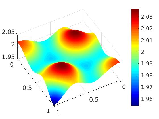
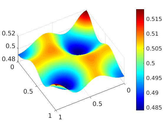
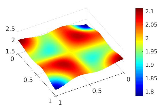
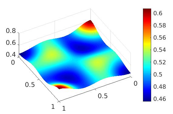
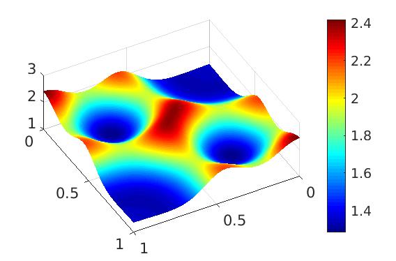
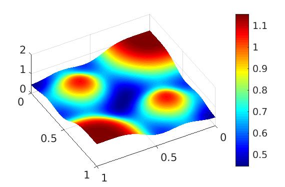
Figure 1. Test case 2: Evolution of the densities $u_{1}$ (left column) and $u_{2}$ (right column) at times $t=0.5$, $1$, $2$ and $4$ (from top to bottom).

8.4. Test case 3: Spatial niche and repulsive potential

In this section, we consider the two-species SKT model with environmental potential, i.e., we add to equation (1) a smooth function $\phi(x)$,

$$\partial_{t}u_{i}-\operatorname{div}\bigg{(}\sum_{j=1}^{n}A_{ij}(u)\nabla u_{j}-d_{i}u_{i}\nabla\phi\bigg{)}=f_{i}(u)\quad\mbox{in }\Omega,\ t>0,\ i=1,\ldots,n,$$

where $d_{i}>0$ and $A_{ij}(u)$ is given by (2) for $i$, $j=1,\ldots,n$. We adapt the definition of the finite-volume scheme (9)–(12) by defining the fluxes as

$$\mathcal{F}_{i,K,\sigma}^{k}=-\bigg{(}\sum_{j=1}^{n}\tau_{\sigma}A_{ij}(u^{k}_{\sigma})\textrm{D}_{K,\sigma}u^{k}_{j}-d_{i}u^{k}_{i,\sigma}\textrm{D}_{K,\sigma}\phi\bigg{)}\quad\mbox{for }K\in{\mathcal{T}},\ \sigma\in{\mathcal{E}}_{K},$$

where

$$\phi_{K}=\frac{1}{\operatorname{m}(K)}\int_{K}\phi(x)\,dx\quad\mbox{for }K\in{\mathcal{T}}.$$

By adapting the proof of Theorem 1, we obtain the following discrete entropy inequality:

$$(1- C_{f}\Delta t)H[u^{k}]+\frac{c_{A}}{2}\Delta t\sum_{i=1}^{n}\sum_{\sigma\in{\mathcal{E}}}\tau_{\sigma}(\mathrm{D}_{\sigma}u_{i}^{k})^{2}$$

$$\leq H[u^{k-1}]+\frac{\Delta t}{2c_{A}}\sum_{i=1}^{n}d_{i}^{2}\sum_{\sigma\in{\mathcal{E}}}\tau_{\sigma}(\mathrm{D}_{\sigma}\phi)^{2}+C_{f}\Delta t\operatorname{m}(\Omega),\quad k\geq 1.$$

This estimate ensures the existence of a nonnegative solution to the scheme and its convergence to the continuous model.

Now we consider a mesh of $\Omega=(0,1)^{2}$ composed of $3584$ triangles and choose the same values for the diffusion and Lotka–Volterra constants as in Section 8.3. Furthermore, we take $d_{1}=d_{2}=2$ and the environmental potential

$$\phi(x,y)=\exp\big{(}-2\big{(}(x-0.5)^{2}+(y-0.5)^{2}\big{)}\big{)}.$$

The inital data is defined according to

$$u_{1}^{0}(x,y) =2+0.31g(x-0.25,y-0.25)+0.31g(x-0.75,y-0.75),$$

$$u_{2}^{0}(x,y) =0.5+0.2g(x-0.5,y-0.5),$$

where the function $g$ is given by (31).

In Figure 2 we illustrate the creation of an ecological niche. We observe that species 2 creates a niche around the point $(0.5,0.5)$ to avoid extinction even when dominated by species 1. This figure can be seen as a two-dimensional variant of the numerical experiments done in [22, Section 3.2, case I].

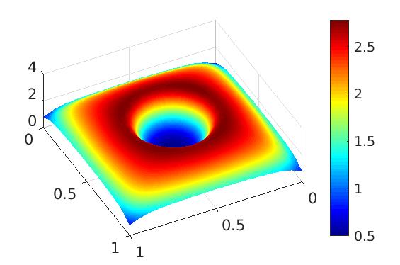
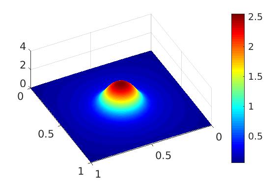
Figure 2. Test case 3: Density $u_{1}$ (left) and $u_{2}$ (right) at time $t=0.5$.

8.5. Test case 4: Convergence to a constant steady state

In this last numerical experiment, we illustrate Theorem 3. In particular, we consider the SKT model with three species and without source terms. We choose the values $a_{10}=1$, $a_{20}=5$, $a_{30}=7$, $a_{11}=a_{21}=a_{31}=1$, $a_{12}=3$, $a_{22}=2$, $a_{32}=1$, $a_{13}=4$, $a_{23}=4/3$, $a_{33}=2$, with $\pi_{1}=1$, $\pi_{2}=3$ and $\pi_{3}=4$ and the initial datum

$$u_{1}^{0}(x,y) =0.5\mathbf{1}_{(0.2,0.4)^{2}}(x,y),$$

$$u_{2}^{0}(x,y) =0.7\mathbf{1}_{(0.6,0.8)\times(0.2,0.4)}(x,y),$$

$$u_{3}^{0}(x,y) =\mathbf{1}_{(0.4,0.6)\times(0.6,0.8)}(x,y).$$

In Figure 3, we present in semilogarithmic scale the behavior of the relative Boltzmann entropy

$$H[u^{k}|\bar{u}]=\sum_{i=1}^{n}\sum_{K\in{\mathcal{T}}}\operatorname{m}(K)\pi_{i}\bigg{(}u^{k}_{i,K}\log\bigg{(}\frac{u^{k}_{i,K}}{\bar{u}_{i}}\bigg{)}+\bar{u}_{i}-u^{k}_{i,K}\bigg{)},$$

where $\bar{u}_{i}=\operatorname{m}(\Omega)^{-1}\int_{\Omega}u^{0}_{i}(x)\,dx$ for $i=1,\ldots,n$, and the squared weighted $L^{1}$ norm

$$\sum_{i=1}^{n}\pi_{i}\|u^{k}_{i}-\bar{u}_{i}\|^{2}_{0,1,{\mathcal{T}}},$$

versus time (with final time $T=1$) for a mesh of $\Omega=(0,1)^{2}$ composed of $3584$ triangles. As proved in Theorem 3, we observe an exponential convergence rate of the solutions to the scheme towards the constant steady state.

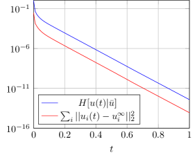
Figure 3. Test case 4: Evolution of the relative Boltzmann entropy and the squared weighted $L^{1}$ norm in semilogarithmic scale.

Appendix A Computation of the constant $C_{f}$ given by (21)

We claim that the Lotka–Volterra terms (3) satisfy Hypothesis (H6) with $C_{f}$ given by (21). For this, define $g(s)=s(\log s-1)+1$ for $s\geq 0$. Then, for $u=(u_{1},\ldots,u_{n})\in(0,\infty)^{n}$, using $-u_{i}\log u_{i}\leq e^{-1}$, we have

$$\sum_{i=1}^{n}f_{i}(u)\pi_{i}\log(u_{i}) \leq\sum_{i=1}^{n}\pi_{i}b_{i0}g(u_{i})+\sum_{i=1}^{n}\pi_{i}b_{i0}u_{i}-\sum_{i=1}^{n}\pi_{i}u_{i}\log(u_{i})\sum_{j=1}^{n}b_{ij}u_{j}$$

$$\leq h(u)\max_{i=1,\ldots,n}b_{i0}+\sum_{i=1}^{n}\pi_{i}b_{i0}u_{i}+\frac{1}{e}\sum_{i=1}^{n}\pi_{i}\sum_{j=1}^{n}b_{ij}u_{j}.$$

Reordering the terms in the last sum yields

$$\sum_{i=1}^{n}f_{i}(u)\pi_{i}\log(u_{i}) \leq h(u)\max_{i=1,\ldots,n}b_{i0}+\sum_{i=1}^{n}\pi_{i}u_{i}\bigg{(}b_{i0}+\frac{1}{e\pi_{i}}\sum_{j=1}^{n}\pi_{j}b_{ji}\bigg{)}$$

$$\leq h(u)\max_{i=1,\ldots,n}b_{i0}+\max_{i=1,\ldots,n}\bigg{(}b_{i0}+\frac{1}{e\pi_{i}}\sum_{j=1}^{n}\pi_{j}b_{ji}\bigg{)}\sum_{i=1}^{n}\pi_{i}u_{i}.$$

Now, we simply notice that the inequality $s\leq(1+g(s))/\log 2$ holds true for all $s\geq 0$. Then, for $s=\sum_{i=1}^{n}\pi_{i}u_{i}$, we infer that

$$\sum_{i=1}^{n}f_{i}(u)\pi_{i}\log(u_{i}) \leq(1+h(u))\max_{i=1,\ldots,n}b_{i0}+\frac{1+h(u)}{\log 2}\max_{i=1,\ldots,n}\bigg{(}b_{i0}+\frac{1}{e\pi_{i}}\sum_{j=1}^{n}\pi_{j}b_{ji}\bigg{)}$$

$$\leq\frac{2}{\log 2}\max_{i=1,\ldots,n}\bigg{(}b_{i0}+\frac{1}{e\pi_{i}}\sum_{j=1}^{n}\pi_{j}b_{ji}\bigg{)}(1+h(u))=C_{f}(1+h(u)).$$

which shows the claim.

References

- [1] A. A. H. Oulhaj. Numerical analysis of a finite volume scheme for a seawater intrusion model with cross-diffusion in an unconfined aquifer. Numer. Meth. Partial Diff. Eqs. 34 (2018), 857–880.
- [2] B. Andreianov, M. Bendahmane, and R. Ruiz Baier. Analysis of a finite volume method for a cross-diffusion model in population dynamics. Math. Models Meth. Appl. Sci. 21 (2011), 307–344.
- [3] J. Barrett and J. Blowey. Finite element approximation of a nonlinear cross-diffusion population model. Numer. Math. 98 (2004), 195–221.
- [4] M. Beauregard and J. Padget. A variable nonlinear splitting algorithm for reaction diffusion systems with self- and cross-diffusion. Numer. Meth. Partial Diff. Eqs. 35 (2019), 597–614.
- [5] M. Bessemoulin-Chatard, C. Chainais-Hillairet, and F. Filbet. On discrete functional inequalities for some finite volume schemes. IMA J. Numer. Anal. 35 (2015), 1125–1149.
- [6] A. Blanchet, J. Dolbeault, and B. Perthame. Two-dimensional Keller–Segel model: Optimal critical mass and qualitative properties of the solutions. Electron. J. Diff. Eqs. 2006 (2006), article 44, 32 pages.
- [7] C. Cancès, C. Chainais-Hillairet, M. Herda, and S. Krell. Large time behavior of nonlinear finite volume schemes for convection-diffusion equations. SIAM J. Numer. Anal. 58 (2020), 2544–2571.
- [8] C. Cancès and B. Gaudeul. A convergent entropy diminishing finite volume scheme for a cross-diffusion system. SIAM J. Numer. Anal. 58(5) (2020), 2684–2710.
- [9] J. A. Carrillo, S. Hittmeir, and A. Jüngel. Cross-diffusion and nonlinear diffusion preventing blow up in the Keller–Segel model. Math. Models Meth. Appl. Sci. 22 (2012), 1250041, 25 pages.
- [10] C. Chainais-Hillairet, J.-G. Liu, and Y.-J. Peng. Finite volume scheme for multi-dimensional drift-diffusion equations and convergence analysis. ESAIM Math. Model. Numer. Anal. 37 (2003), 319–338.
- [11] L. Chen and A. Jüngel. Analysis of a multi-dimensional parabolic population model with strong cross-diffusion. SIAM J. Math. Anal. 36 (2004), 301–322.
- [12] L. Chen, E. Daus, and A. Jüngel. Rigorous mean-field limit and cross-diffusion. Z. Angew. Math. Phys. 70 (2019), no. 122, 21 pages.
- [13] X. Chen, E. Daus, and A. Jüngel. Global existence analysis of cross-diffusion population systems for multiple species. Arch. Ration. Mech. Anal. 227 (2018), 715–747.
- [14] D. Clark. Short proof of a discrete Gronwall inequality. Discrete Appl. Math. 16 (1987), 279–281.
- [15] K. Deimling. Nonlinear Functional Analysis. Springer, Berlin, 1985.
- [16] R. Eymard, T. Gallouët, and R. Herbin. Finite volume methods. In: P. G. Ciarlet and J.-L. Lions (eds.). Handbook of Numerical Analysis 7 (2000), 713–1018.
-
[17]
R. Eymard, T. Gallouët, and R. Herbin.
Finite Volume Methods.
Schemes and Analysis. Course at the University of Wroclaw. Lecture notes, 2008.
Available at
http://www.math.uni.wroc.pl/~olech/courses/skrypt_Roberta_wroclaw.pdf. - [18] F. Filbet and M. Herda. A finite volume scheme for boundary-driven convection-diffusion equations with relative entropy structure. Numer. Math. 137 (2017), 535–577.
- [19] G. Galiano, M. Garzón, and A. Jüngel. Analysis and numerical solution of a nonlinear cross-diffusion system arising in population dynamics. RACSAM Rev. R. Acad. Cien. Ser. A 95 (2001), 281–295.
- [20] G. Galiano, M. Garzón, and A. Jüngel. Semi-discretization in time and numerical convergence of solutions of a nonlinear cross-diffusion population model. Numer. Math. 93 (2003), 655–673.
- [21] T. Gallouët and J.-C. Latché. Compactness of discrete approximate solutions to parabolic PDEs – Application to a turbulence model. Commun. Pure Appl. Anal. 11 (2012), 2371–2391.
- [22] G. Gambino, M. Lombardo, and M. Sammartino. A velocity-diffusion method for a Lotka–Volterra system with nonlinear cross and self-diffusion. Appl. Numer. Math. 59 (2009), 1059–1074.
- [23] D. Grebenkov and B.-T. Nguyen. Geometrical structure of Laplacian eigenfunctions. SIAM Rev. 55 (2013), 601–667.
- [24] G. Grün and M. Rumpf. Nonnegativity preserving convergent schemes for the thin film equation. Numer. Math. 87 (2000), 113–152.
- [25] E. Hairer, C. Lubich, and G. Wanner. Geometric Numerical Integration. Second edition. Springer, Berlin, 2006.
- [26] A. Jüngel. The boundedness-by-entropy method for cross-diffusion systems. Nonlinearity 28 (2015), 1963–2001.
- [27] A. Jüngel. Entropy Methods for Diffusive Partial Differential Equations. BCAM Springer Briefs, Springer, 2016.
- [28] A. Jüngel and A. Zurek. A finite-volume scheme for a cross-diffusion model arising from interacting many-particle population systems. In: R. Klöfkorn, E. Keilegavlen, F. Radu, and J. Fuhrmann (eds.). Finite Volumes for Complex Applications IX. Springer, Cham, 2020, pp. 223-231.
- [29] A. Mielke. Geodesic convexity of the relative entropy in reversible Markov chains. Calc. Var. Partial Diff. Eqs. 48 (2013), 1–31.
- [30] H. Murakawa. A linear finite volume method for nonlinear cross-diffusion systems. Numer. Math. 136 (2017), 1–26.
- [31] N. Shigesada and K. Kawazaki. Biological Invasions: Theory and Practise. Oxford University Press, 1997.
- [32] N. Shigesada, K. Kawasaki, and E. Teramoto. Spatial segregation of interacting species. J. Theor. Biol. 79 (1979), 83–99.
- [33] Z. Sun, J. A. Carrillo, and C.-W. Shu. An entropy stable high-order discontinuous Galerkin method for cross-diffusion gradient flow systems. Kinetic Related Models 12 (2019), 855–908.
- [34] C. Tian, Z. Lin, and M. Pedersen. Instability induced by cross-diffusion in reaction-diffusion systems. Nonl. Anal. Real World Appl. 11 (2010), 1036–1045.