Generalized Posteriors in Approximate Bayesian Computation

Abstract

Complex simulators have become a ubiquitous tool in many scientific disciplines, providing high-fidelity, implicit probabilistic models of natural and social phenomena. Unfortunately, they typically lack the tractability required for conventional statistical analysis. Approximate Bayesian computation (abc) has emerged as a key method in simulation-based inference, wherein the true model likelihood and posterior are approximated using samples from the simulator. In this paper, we draw connections between abc and generalized Bayesian inference (gbi). First, we re-interpret the accept/reject step in abc as an implicitly defined error model. We then argue that these implicit error models will invariably be misspecified. While abc posteriors are often treated as a necessary evil for approximating the standard Bayesian posterior, this allows us to re-interpret abc as a potential robustification strategy. This leads us to suggest the use of gbi within abc, a use case we explore empirically.

1 Introduction

Approximate Bayesian computation (abc) is a family of techniques for computing approximate Bayesian posteriors in the presence of intractable likelihoods (see e.g. Beaumont et al., 2002; Fan and Sisson, 2018; Beaumont, 2019). Accordingly, such methods are particularly attractive when one is confronted with complex physical simulators. Suppose we are given a probabilistic simulator $f(\cdot\mid\theta)$ parameterized by $\theta\in\Theta$ and defining a probability distribution on $\mathcal{X}$. Assuming that $\int_{\mathcal{X}}f(x\mid\theta)\,\mathrm{d}x=1$, this simulator also defines a likelihood. If we have observations $y$ and a prior belief $p(\theta)$, the standard Bayesian approach is to update our belief according to Bayes’ rule, rCl p(θ∣y) & ∝ f(y ∣θ)p(θ). Clearly, this approach is infeasible for general simulation engines. While we can sample $x\sim f(\cdot\mid\theta)$ for any $\theta\in\Theta$, evaluating $f(y\mid\theta)$ for a given $y$ and $\theta$ is in general not possible. The picture is further complicated by misspecification: the simulator $f(\cdot\mid\theta)$ will seldom describe the true data generating process $y\sim p^{*}(\cdot)$ perfectly. While many approaches exist for tackling this intractable likelihood problem (see e.g. Cranmer et al., 2020, for a recent overview), almost all of them rely on the assumption that the likelihood model defined through the simulator is correctly specified. In the following, we will show how generalized Bayesian inference (gbi) can be used to design abc algorithms robust to misspecification.

Operationally, abc describes the following algorithm: first, sample $\theta\sim p(\theta)$; next, sample $x\mid\theta\sim f(x\mid\theta)$ by running the simulator with parameter $\theta$; lastly, weight the disagreement between $x$ and the observed data $y$ by comparing low-dimensional summary statistics, $\eta(x)$ and $\eta(y)$, as judged by some probability kernel function $K_{h}(\|\eta(x)-\eta(y)\|)$ with bandwidth $h$. This induces an augmented distribution $p(\theta,x\mid y)$, a marginal of which yields an approximation to the Bayesian posterior rCl p(θ∣y) ≈p_abc(θ∣y) :=∫p(θ, x ∣y)   dx ∝∫K_h(∥η(x)-η(y)∥)f(x—θ)p(θ)   dx. The logic in (1) is immediate: the smaller the bandwidth $h$ of the kernel, the more accurate our approximation to the true posterior will be. On the other hand, smaller bandwidths result in down-weighting or discarding more of the simulator outputs. Further, one needs to choose a summary statistic $\eta$ that is “as sufficient as possible” to optimally use all information in the data. This tension between the theoretically optimal and the practically feasible is a recurrent theme within the literature on abc (e.g. Blum et al., 2013).

In the current paper, we use recent insights from gbi (see e.g. Grünwald, 2012; Bissiri et al., 2016; Jewson et al., 2018; Guedj, 2019; Knoblauch et al., 2019) to form a new perspective on these issues. The first key step is the reinterpretation of the kernel $K_{h}$ as the measurement error model for the true data $y$. Unlike the standard interpretation of $K_{h}$ in abc, this suggests that larger bandwidths $h$ could actually be beneficial for more robust inferences. More precisely, when the simulator is a poor description of $y$ for any value of $\theta$, an explicit model of the noise may robustify inference. As the noise models themselves will also be misspecified, we further draw a natural connection to gbi: using generalizations of the Bayesian principle, one can circumvent the drawbacks of having a substantially misspecified noise model. In summary, rather than treating abc as a necessary evil for approximating the standard Bayesian posterior, we re-interpret it as a flexible robustification strategy.

2 Bayesian calibration of stochastic simulators

Traditional approaches for calibrating stochastic simulators assume that the model is well-specified, inherent in the commonly stated aim to approximate the posterior of the simulator

$$p(\theta\mid y)\propto f(y\mid\theta)p(\theta).$$

However, if $y$ is a real-world observation, it is rarely safe to assume it is drawn from the simulator. On the contrary, it is reasonable to assume that the simulator is misspecified to a significant degree—either because of measurement error in the data collection process or because of the modelling challenge of capturing the true dynamics. The latter is of particular importance in the simulation of e.g. social dynamics and economic models, where any simulation-based method can at best provide a simplified view of real-world processes. Consequently, we suggest augmenting the simulation model to incorporate measurement error in $y$. Formally, we assume that there exists a measurement error (or noise) model $g$ such that the true data generating process $p^{*}\in\{p(\cdot\mid\theta);\theta\in\Theta\}$ is given by

$$p(y\mid\theta)=\int_{\mathcal{X}}g(y\mid x)f(x\mid\theta)\,\mathrm{d}x\quad\text{and}\quad p(\theta\mid y)\propto p(y\mid\theta)p(\theta).$$ (1)

While the error model $g$ could in principle depend on $\theta$ as well, we do not consider this case in the remainder. In practice of course, the “true” error distribution $g$ is also unknown, so that relatively coarse approximations will have to be used instead. For this reason we advocate the use of generalized Bayesian inference (gbi) (e.g. Bissiri et al., 2016, and Appendix A) within abc to obtain robust posterior inference.

2.1 A general view on likelihood-free inference

gbi extends the logic of Bayesian belief updating from a likelihood function to an arbitrary loss $\ell$. Its main practical use lies in addressing robustness and misspecification (see e.g. Hooker and Vidyashankar, 2014; Ghosh and Basu, 2016; Jewson et al., 2018; Knoblauch et al., 2018). Replacing the measurement error distribution with a general loss $\ell$ and plugging it into the relevant abc formulation yields

$$p_{\ell}(\theta\mid y)\propto\int\exp{\{-w\cdot{\ell}(y;x)\}}f(x\mid\theta)p(\theta)\,\mathrm{d}x.$$ (2)

The above generalizes standard abc: instead of a probability kernel $K_{h}$, one may now use any loss function $\ell$ to assess the discrepancy between $x$ and $y$. The weight $w>0$ can be chosen to adjust the influence of a given loss on the posterior, and we illustrate this in LABEL:fig:weights using a toy example which is described below in Section 3.

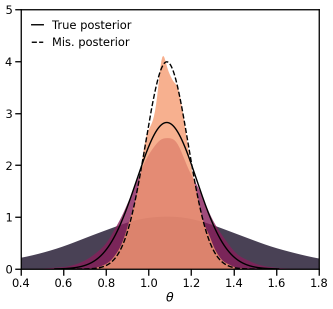
fig:weights [Soft-threshold abc ]    [Wasserstein abc        ]

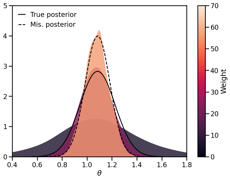
Figure 1: Abc posteriors targeting (2) using a soft-threshold loss based on sufficient statistics $\eta(x)$, and a Wasserstein distance loss on the full model output $x$.

2.2 Links to approximate Bayesian computation

If the error distribution $g(y\mid x)$ of (1) is identical to the kernel $K_{h}(\|\eta(x)-\eta(y)\|)$, the corresponding abc algorithm recovers the correct posterior based on the likelihood $p(y\mid\theta)$ (rather than $f(y\mid\theta)$). While this argument for interpreting the usual abc kernels as error distributions was previously made by Wilkinson (2013), it seems implausible that the correct measurement error of a complex simulator can be expressed in terms of a difference of low-dimensional summary statistics via $K_{h}$. Regardless, under this assumption one can substitute into (2) the unit weight $w=1$ and the likelihood

$$\ell(y;x)=-\log K_{h}(\lVert\eta(x)-\eta(y)\rVert)$$ (3)

to recover not only the abc posterior $p_{\lx@glossaries@gls@link{acronym}{abc}{\leavevmode\textsc{abc}}}(\theta\mid y)$, but also the correct posterior based on the likelihood $p(y\mid\theta)$ of (1). Doing so also demonstrates that the set of possible gbi posteriors in (2) contains all standard as well as a range of new and generalized abc posteriors, suggesting the traditional form (1) of abc posteriors is an artificial restriction.

Some popular abc kernels gain new interpretations viewed through this lens. For example, $K_{h}$ is often taken to be a Gaussian kernel, implying through (3) the loss ${\ell}(y;x)\propto\frac{1}{2h^{2}}\lVert\eta(x)-\eta(y)\rVert^{2}$. This is a reasonable choice for $\ell$ whenever the (additive) observation noise on the summary statistics is at least approximately $\mathcal{N}(0,h^{2})$ distributed. On the other hand, if $\mathcal{N}(0,h^{2})$ is a poor description of the error model, then gbi robustification strategies could be deployed within abc (e.g. Knoblauch et al., 2018; Boustati et al., 2020). In contrast, the appeal of many popular abc kernels is greatly reduced when viewed in this light. For example, hard-threshold kernels given by indicator functions such as $K_{\varepsilon}(x,y)=\mathbbm{1}\{\lVert\eta(x)-\eta(y)\rVert<\varepsilon\}$ would correspond to a compactly supported and discontinuous noise model $g(y\mid x)=K_{\varepsilon}(x,y)$. In virtually any other application, this choice of error model would be unconventional—yet it is commonplace in abc.

We submit that abc can elegantly address misspecification by leveraging gbi: Under the gbi paradigm, we make more reasonable choices for $K_{h}$—choices that more accurately reflect the measurement error $g(y\mid x)$—that would be unnatural or even forbidden by the functional form of $K_{h}$ within standard abc. While some pre-existing work on abc has taken small steps towards special cases of this generalization, these approaches do not consider the framework in its full generality (see e.g. Park et al., 2016; Ridgway, 2017).

2.3 Sampling from ABC posteriors

Given a choice of loss $\ell(y;x)$, gbi requires us to compute expectations with respect to the posterior (2). The most common approaches are sampling algorithms based on the pseudo-marginal method (Beaumont, 2003; Andrieu et al., 2009). Such samplers follow a Markov chain Monte Carlo (mcmc) approach: given a point $\{\theta,\ell(y;x)\}$, propose $\theta^{\prime}\sim\mathcal{N}(\cdot;\theta,\lambda)$—a Gaussian centered at $\theta$ with variance $\lambda$—and $\ell(y;x^{\prime})$ with $x^{\prime}\sim f(\cdot\mid\theta)$ and accept with probability

$$a(\theta,\theta^{\prime})=\min\left\{1,\frac{e^{-w\cdot{\ell}(y;x^{\prime})}p(\theta^{\prime})}{e^{-w\cdot{\ell}(y;x)}p(\theta)}\right\},$$

otherwise remain in the same state. An important result in mcmc theory is that the respective Markov chain will indeed converge to the desired target distribution (2). The resulting algorithm can be seen as a generalization of the abc-mcmc scheme of Marjoram et al. (2003).

While we restrict our attention to mcmc methods, the suggested gbi target (2) is amenable to other popular abc algorithms, e.g. importance sampling as proposed by Park et al. (2016) or smc-abc (Sisson et al., 2007) using, for instance, the methods of Fearnhead et al. (2008); Schmon et al. (2019).

3 Simulation Study

Throughout, we study the toy example of Frazier, David T. and Robert, Christian P. and Rousseau, Judith (2020). In this example, we assume that the true generative model comes from the family with likelihood $p(x\mid\theta)=\mathcal{N}(x;\theta,2)$, that is, a Gaussian density with mean $\theta$ and variance $2$. We generate 100 data points according to an unobserved $\theta^{*}=1$, i.e. $p^{*}(y)=p(y\mid\theta^{*})$, where our prior beliefs about this parameter are given by $p(\theta)=\mathcal{N}(\theta;0,25)$. Instead of reflecting the correct likelihood model, our simulator is misspecified and assumes that $y$ was generated from $f(\cdot\mid\theta)=\mathcal{N}(x;\theta,1)$. Note that this means the true error has a distribution given by $g(y\mid x)=\mathcal{N}(y;x,1)$.

Our aim is to investigate the impact of the loss function on performance, as a judicious choice can not only help target the true posterior distribution, but may also substantially reduce the computational burden. This highlights the use of gbi within abc for improved robustness and computational efficiency as outlined in Section 2.2.

Throughout, we focus on abc-mcmc algorithms (see e.g. Fan and Sisson, 2018) with soft-threshold losses, as we found this approach to perform very reliably. Where summary statistics are used, we employ the mean and variance $\eta=(\eta_{1},\eta_{2})$, which are sufficient for the normal distribution. The losses we consider take the form $\ell(y;x)=\frac{1}{M}\sum_{i=1}^{M}\tilde{\ell}(y;x_{i})$ where $x_{i}\overset{iid}{\sim}f(\cdot\mid\theta)$ and $M$ denotes the number of simulator draws or particles. For $\tilde{\ell}$, we consider: the squared 2-norm applied to a difference of sufficient statistics, i.e. $\lVert\eta(x_{i})-\eta(y)\rVert^{2}$, which we call st-abc; the maximum mean discrepancy (mmd) loss as used in k2-abc (Park et al., 2016); and the Wasserstein distance, which we call w-abc (note that our approach differs from that of Bernton et al., 2019).

3.1 Solving the exact problem

Formulating simulation-based inference as a latent variable model as we propose in (1) might suggest that the aim of abc lies in an accurate modelling of the error distribution $g(y\mid x)$, i.e. finding $w\cdot\ell(y;x)\approx-\log g(y\mid x)$. However, in practice considerations such as computational cost and robustness may well trump the benefits of modelling $g(y\mid x)$ exactly. In order to test this hypothesis, we leverage the fact that the true error distribution in our toy model is known and employ a pseudo-marginal algorithm (Beaumont, 2003; Andrieu et al., 2009) to sample exactly from the correct posterior $p(\theta\mid y)$.

We tune this algorithm so as to maximize the effective sample size (ess) (using the ess function from the ArviZ library, Kumar et al. 2019) given a fixed budget of draws from the simulator. In particular, we choose the number of draws per iteration (this turns out to be more efficient than taking just a single sample, see e.g. Pitt et al., 2012; Doucet et al., 2015; Schmon et al., 2020) so that the acceptance rate is around $25\%$ (Schmon et al., 2020). As a comparison we take the st-abc algorithm described above. The abc algorithm uses an average of losses based on 15 samples, which improves the ess for a given number of calls to the simulator (see LABEL:fig:robust_ess_experiment), and is tuned so that it approximately targets the true posterior, as shown in LABEL:fig:abc_pmcmc in Appendix C. Further, we carry out a two sample Kolmogorov–Smirnov test on a subset of samples obtained from both methods, which demonstrates no significant difference between the distributions. Given a budget of 1.5 million simulator calls, we compute the ess of both the pseudo-marginal chain and the abc chain. While the pseudo-marginal algorithm achieves an ess of $\approx 2723$, abc-mcmc results in an ess of more than $11080$—making it more than four times as efficient. This has an important implication: while modelling the error distribution exactly may target the correct posterior, computational considerations may still favour alternative approaches.

3.2 General loss functions

The generalized posterior (2) allows for consideration of a wide variety of losses with diverse properties. We compare a selection of losses against the following criteria:

• Computational cost. Calls to most simulators of interest are expensive. Algorithms should make efficient use of simulations, perhaps through use of $M>1$ particles.
  

• Misspecification robustness. Algorithms offering stable performance under high degrees of misspecification are to be preferred.
  

Criterion i) is addressed in Figure 2. In this experiment, each algorithm run draws 3 million samples from the simulator, effectively fixing the computational cost. Those samples are spent on 3 million mcmc iterations with $M=1$ particle, 1.5 million mcmc iterations with $M=2$ particles, and so on. Finally, the efficiency is measured by the ess of the mcmc chain generated. For low numbers of particles, k2-abc and w-abc are vastly more efficient than the more conventional st-abc. Both k2-abc and w-abc lose efficiency through any amount of loss-averaging. In contrast, the ess of st-abc is maximised at around 15-25 particles. Turning to criterion ii), in Figure 2 we explore the behaviour of the algorithms under misspecification. Here, we have assumed that the true data generating process is $\mathcal{N}(1,\sigma^{2})$ and report the posterior mean of the abc-mcmc samples of each algorithm. Further details are provided in Appendix B. In agreement with Figure 2, st-abc produces posterior means of a far higher variance than the other losses, even using $M=2$ particles (see Appendix B). Using 64 particles improves performance for st-abc—and yet, both k2-abc and w-abc still outperform it at every level of misspecification using only a single particle.

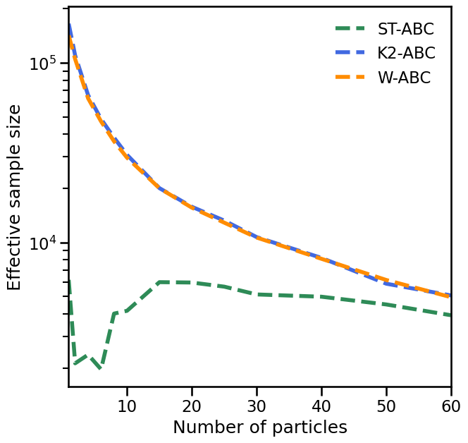
fig:robust_ess_experiment [The effective sample size as a function of $M$, the number of particles.]     [The posterior mean as a function of the degree of misspecification of the model.]

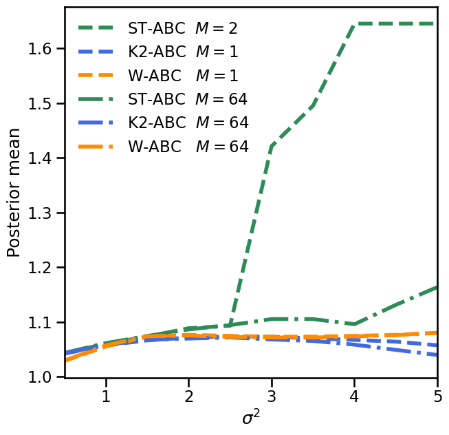
Figure 2: Two comparisons of abc algorithms with a soft-threshold loss (st-abc), an mmd loss (k2-abc), and a Wasserstein loss (w-abc).

4 Discussion

We have introduced a unifying view for likelihood-free inference methods by relating approximate Bayesian computation (abc) to generalized Bayesian inference (gbi). Using the full expressivity of arbitrary loss functions allows us to re-interpret existing methods, but also suggests new promising directions for future research on abc. We believe that this approach will broaden the scope of applicability for abc algorithms, particularly in applications where simulators are known to be inexact representations of the real world data-generating mechanism for $y$.

JK is funded by the EPSRC grant EP/L016710/1 as part of the Oxford-Warwick Statistics Programme (OxWaSP). JK is additionally funded by the Facebook Fellowship Programme and the London Air Quality project at the Alan Turing Institute for Data Science and AI as part of the Lloyd’s Register Foundation programme on Data Centric Engineering. This work was furthermore supported by The Alan Turing Institute for Data Science and AI under EPSRC grant EP/N510129/1 in collaboration with the Greater London Authority.

Appendix A Generalized Bayesian Inference

Generalized Bayesian inference (gbi) is a family of Bayes-like methods based around Gibbs posteriors. These methods can be justified from multiple angles, including the PAC-Bayesian perspective (see Guedj, 2019, for a recent survey), the so-called Safe Bayes motivation of Grünwald (2012), a discrepancy-based perspective on Bayesian inference (see Jewson et al., 2018) as well as an optimization-centric view (see Knoblauch et al., 2019). Perhaps most in line with the traditional Bayesian view is the conceptual justification of Bissiri et al. (2016). Under a restrictive definition of coherent belief updates, the authors show that a Bayes-like update rule is a valid inferential device for general loss functions. In particular, given a loss function $\ell:\Theta\times\mathcal{X}\to\mathbb{R}$ with parameter space $\Theta$ and a prior belief $p(\theta)$ over $\Theta$, one can show that a coherent belief update in the presence of an observation $y\in\mathcal{X}$ is given by the Bayes-like operation

$$p_{\ell}(\theta\mid y)\propto\exp(-\ell(y;\theta))p(\theta).$$

Here, $p_{\ell}(\theta\mid y)$ is a coherent belief whenever the normalization constant $\int\exp(-\ell(y;\theta))p(\theta)\mathrm{d}\theta$ is finite. This framework is appealing as it provides a new conceptual justification for belief distributions that have been studied elsewhere, particularly in the PAC-Bayesian literature.

Appendix B Further details to simulation study

In Figure 2 the true data generating process is a $\mathcal{N}(1,\sigma^{2})$, while the model is $\mathcal{N}(\theta,1)$. Each experiment comprises drawing a new observation $y_{\sigma^{2}}=1+\sigma\xi$, where $\xi\sim\mathcal{N}(0,1)$; the seed is held fixed so that $\xi$ is constant across observations. Then $3\times 10^{6}$ Markov chain Monte Carlo (mcmc) samples are generated from the respective sampler. The dashed lines show the performance for a single particle, with the exception of soft-threshold approximate Bayesian computation (abc), which exhibited too high variance in the effective sample size (ess) estimate with only a single particle and so two particles were used. Even with two particles, for reasonable levels of misspecification ($\sigma^{2}>2.5$) the ess for st-abc diminished extremely quickly. Thus, not only do the posterior means drift further from the true value as misspecification increases, but the algorithm itself ceases to function reliably. This shortcoming was not present in any other algorithm tested.

In advance of running the experiments in LABEL:fig:robust_ess_experiment, each algorithm was tuned by setting its weight to approximately target the true posterior. In that way, every algorithm tested could have been used to perform the same inferential task. Once the weights were set, to verify the algorithms were producing samples approximately from the same distribution, sub-samples of length 150 were randomly sampled from each posterior chain and compared using a two-sample Kolmogorov–Smirnov test. As the null hypothesis was not rejected at the 0.1 level for 5 different observations $y$, we found the posteriors satisfactorily close.

fig:abc_pmcmc

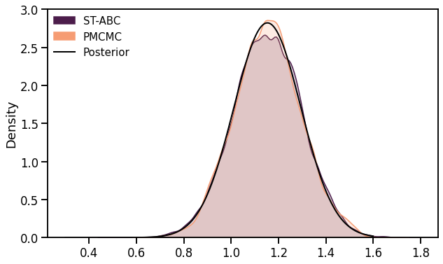
Figure 3: Abc and a pseudo-marginal algorithm compared to the true posterior. The sampled posteriors are very close to the intended target distribution.

Appendix C Links to hidden Markov models

The view of a latent variable model with measurement error is one that is commonly used in the field of hidden Markov models. Following our previous notation, models consist of a hidden Markov chain evolving according to

$$x_{i}\mid x_{i-1}\sim f(\cdot\mid x_{i-1},\theta),\quad y_{o,i}\mid x_{i}\sim g(\cdot\mid x_{i},\theta).$$ (4)

Denote the observed time series $y=(y^{(1)},\ldots,y^{(n)})$, we can then recover expression (2) by setting

$$p(\theta\mid y)=\int_{\mathcal{X}}g_{\theta}(y\mid x)f(x\mid\theta)\mathrm{d}x\,p(\theta),$$

with $f_{1}(x^{(1)}\mid x^{(0)},\theta)=f_{1}(x^{(1)}\mid\theta)$ and

$$f(x\mid\theta)=\prod_{i=1}^{n}f_{i}(x^{(i)}\mid x^{(i-1)},\theta),\quad g_{\theta}(y\mid x)=\prod_{i=1}^{n}g_{i}(y^{(i)}\mid x^{(i)},\theta).$$

Particle Markov chain Monte Carlo algorithms (Andrieu et al., 2010) are then designed to target posteriors like (1). Accordingly, they are a possible solution for inference with gbi posteriors whenever the simulator is formulated as a hidden Markov model with known error.

It is noteworthy that for dynamic models particle Markov chain Monte Carlo (pmcmc) and abc are often competitors for solving the same task (e.g. Fasiolo et al., 2016). However, it seems unreasonable to assume that the simulator is well-specified when employing one set of techniques (e.g. abc) while assuming a measurement error model (e.g. pmcmc). In this sense, we suggest to decompose abc analogously to hidden Markov models into signal and noise and to consider abc with appropriately chosen loss as a robust inference method. This is also in line with the results of Fasiolo et al. (2016) who find that pmcmc performs better when the model and noise are well-specified, but may underperform under model misspecification. Perhaps this could be alleviated using robust loss functions in the vein of (2) on their individual noise contributions as proposed Boustati et al. (2020).

References

- Andrieu et al. (2009) Christophe Andrieu, Gareth O Roberts, et al. The pseudo-marginal approach for efficient Monte Carlo computations. The Annals of Statistics, 37(2):697–725, 2009.
- Andrieu et al. (2010) Christophe Andrieu, Arnaud Doucet, and Roman Holenstein. Particle markov chain monte carlo methods. Journal of the Royal Statistical Society: Series B (Statistical Methodology), 72(3):269–342, 2010.
- Beaumont (2003) Mark A Beaumont. Estimation of population growth or decline in genetically monitored populations. Genetics, 164(3):1139–1160, 2003.
- Beaumont (2019) Mark A Beaumont. Approximate Bayesian computation. Annual review of statistics and its application, 6:379–403, 2019.
- Beaumont et al. (2002) Mark A Beaumont, Wenyang Zhang, and David J Balding. Approximate Bayesian computation in population genetics. Genetics, 162(4):2025–2035, 2002.
- Bernton et al. (2019) Espen Bernton, Pierre E. Jacob, Mathieu Gerber, and Christian P. Robert. Approximate Bayesian computation with the Wasserstein distance. Journal of the Royal Statistical Society: Series B (Statistical Methodology), 81(2):235–269, Feb 2019. ISSN 1369-7412. 10.1111/rssb.12312. URL http://dx.doi.org/10.1111/rssb.12312.
- Bissiri et al. (2016) Pier Giovanni Bissiri, Chris C Holmes, and Stephen G Walker. A general framework for updating belief distributions. Journal of the Royal Statistical Society. Series B, Statistical methodology, 78(5):1103, 2016.
- Blum et al. (2013) M. G. B. Blum, M. A. Nunes, D. Prangle, and S. A. Sisson. A Comparative Review of Dimension Reduction Methods in Approximate Bayesian Computation. Statistical Science, 28(2):189–208, May 2013. ISSN 0883-4237. 10.1214/12-sts406. URL http://dx.doi.org/10.1214/12-STS406.
- Boustati et al. (2020) Ayman Boustati, Ömer Deniz Akyildiz, Theodoros Damoulas, and Adam Johansen. Generalized Bayesian Filtering via Sequential Monte Carlo. arXiv preprint arXiv:2002.09998, 2020.
- Cranmer et al. (2020) Kyle Cranmer, Johann Brehmer, and Gilles Louppe. The frontier of simulation-based inference. Proceedings of the National Academy of Sciences, 2020.
- Doucet et al. (2015) Arnaud Doucet, Michael K Pitt, George Deligiannidis, and Robert Kohn. Efficient implementation of Markov chain Monte Carlo when using an unbiased likelihood estimator. Biometrika, 102(2):295–313, 2015.
- Fan and Sisson (2018) Y Fan and SA Sisson. ABC samplers. arXiv preprint arXiv:1802.09650, 2018.
- Fasiolo et al. (2016) Matteo Fasiolo, Natalya Pya, and Simon N Wood. A comparison of inferential methods for highly nonlinear state space models in ecology and epidemiology. Statistical Science, pages 96–118, 2016.
- Fearnhead et al. (2008) Paul Fearnhead, Omiros Papaspiliopoulos, and Gareth O Roberts. Particle filters for partially observed diffusions. Journal of the Royal Statistical Society: Series B (Statistical Methodology), 70(4):755–777, 2008.
- Frazier, David T. and Robert, Christian P. and Rousseau, Judith (2020) Frazier, David T. and Robert, Christian P. and Rousseau, Judith. Model misspecification in approximate bayesian computation: consequences and diagnostics. Journal of the Royal Statistical Society: Series B (Statistical Methodology), 82(2):421–444, 2020. https://doi.org/10.1111/rssb.12356. URL https://rss.onlinelibrary.wiley.com/doi/abs/10.1111/rssb.12356.
- Ghosh and Basu (2016) Abhik Ghosh and Ayanendranath Basu. Robust Bayes estimation using the density power divergence. Annals of the Institute of Statistical Mathematics, 68(2):413–437, 2016.
- Grünwald (2012) Peter Grünwald. The safe Bayesian. In International Conference on Algorithmic Learning Theory, pages 169–183. Springer, 2012.
- Guedj (2019) Benjamin Guedj. A primer on PAC-Bayesian learning. arXiv preprint arXiv:1901.05353, 2019.
- Hooker and Vidyashankar (2014) Giles Hooker and Anand N Vidyashankar. Bayesian model robustness via disparities. Test, 23(3):556–584, 2014.
- Jewson et al. (2018) Jack Jewson, Jim Q Smith, and Chris Holmes. Principles of Bayesian inference using general divergence criteria. Entropy, 20(6):442, 2018.
- Knoblauch et al. (2018) Jeremias Knoblauch, Jack Jewson, and Theodoros Damoulas. Doubly Robust Bayesian Inference for Non-Stationary Streaming Data with -Divergences. In Advances in Neural Information Processing Systems, pages 64–75, 2018.
- Knoblauch et al. (2019) Jeremias Knoblauch, Jack Jewson, and Theodoros Damoulas. Generalized variational inference: Three arguments for deriving new posteriors. arXiv preprint arXiv:1904.02063, 2019.
- Kumar et al. (2019) Ravin Kumar, Colin Carroll, Ari Hartikainen, and Osvaldo A. Martin. ArviZ a unified library for exploratory analysis of Bayesian models in Python. The Journal of Open Source Software, 2019. 10.21105/joss.01143. URL http://joss.theoj.org/papers/10.21105/joss.01143.
- Marjoram et al. (2003) Paul Marjoram, John Molitor, Vincent Plagnol, and Simon Tavaré. Markov chain Monte Carlo without likelihoods. Proceedings of the National Academy of Sciences, 100(26):15324–15328, 2003.
- Park et al. (2016) Mijung Park, Wittawat Jitkrittum, and Dino Sejdinovic. K2-ABC: Approximate Bayesian Computation with Kernel Embeddings. volume 51 of Proceedings of Machine Learning Research, pages 398–407. PMLR, 2016.
- Pitt et al. (2012) Michael K Pitt, Ralph dos Santos Silva, Paolo Giordani, and Robert Kohn. On some properties of Markov chain Monte Carlo simulation methods based on the particle filter. Journal of Econometrics, 171(2):134–151, 2012.
- Ridgway (2017) James Ridgway. Probably approximate Bayesian computation: nonasymptotic convergence of ABC under misspecification. arXiv preprint arXiv:1707.05987, 2017.
- Schmon et al. (2020) S M Schmon, G Deligiannidis, A Doucet, and M K Pitt. Large-sample asymptotics of the pseudo-marginal method. Biometrika, 07 2020. ISSN 0006-3444. 10.1093/biomet/asaa044. URL https://doi.org/10.1093/biomet/asaa044.
- Schmon et al. (2019) Sebastian M. Schmon, Arnaud Doucet, and George Deligiannidis. Bernoulli Race Particle Filters. In Kamalika Chaudhuri and Masashi Sugiyama, editors, Proceedings of Machine Learning Research, volume 89 of Proceedings of Machine Learning Research, pages 2350–2358. PMLR, 16–18 Apr 2019. URL http://proceedings.mlr.press/v89/schmon19a.html.
- Sisson et al. (2007) Scott A Sisson, Yanan Fan, and Mark M Tanaka. Sequential monte carlo without likelihoods. Proceedings of the National Academy of Sciences, 104(6):1760–1765, 2007.
- Wilkinson (2013) Richard David Wilkinson. Approximate Bayesian computation (ABC) gives exact results under the assumption of model error. Statistical applications in genetics and molecular biology, 12(2):129–141, 2013.