Adiabatic theory of the polaron spectral function

Abstract

An analytic theory for the spectral function of electrons coupled with phonons is formulated in the adiabatic limit. In the case when the chemical potential is large and negative $\mu\to-\infty$ the ground state does not have the adiabatic deformation and the spectral function is defined by the standard perturbation theory. In this limit, we use the diagram technique in order to formulate an integral equation for the renormalized vertex. The spectral function was evaluated by solving Dyson’s equation for the self-energy with the renormalized vertex. The moments of the spectral function satisfy the exact sum rules up to the 7th moment. In the case when the chemical potential is pinned at the polaron binding energy the spectral function is defined by the ground state with a nonzero adiabatic deformation. We calculate the spectral function with the finite polaron density in the adiabatic limit. We also demonstrate how the sum rules for higher moments may be evaluated in the adiabatic limit. Contrary to the case of zero polaron density the spectral function with the finite polaron concentration has some contributions which are characteristic for polarons.

I Introduction

The properties of different types of polarons were well studied a long time ago. A number of review articles (see for example AustinMott ; Elliott ; AlexandrovMott ; AlexandrovKrebs ; Mishchenko ; DevreeseAlexandrov ; Klinger1 ) and textbooks Pekar ; KuperWhitfield ; Appel ; AlexandrovDevreese ; AlexandrovMott2 ; Emin is available, which describe the spectroscopic, thermodynamic, kinetic, and other physical properties of polarons. Usually, the polaron theory is used in order to describe electric transport in low mobility crystalline or organic semiconductors (see review article of I. G. Austin, N. F. Mott AustinMott and references therein or more recent papers on organic semiconductors Coropceanu ). It was also successfully used in order to describe equilibrium and photo-induced mid-infrared optical absorption spectra of high-T_c superconductors at low doping Zamboni ; Mihailovic ; Falk ; Calvani . The description is based on the well developed theory of polaron optical absorption Eagles ; Klinger2 ; Reik ; Emin1993 ; AKR_physicaC . The small Jahn-Teller polarons Hock are also found in colossal magnetoresistance manganites Tokura ; Millis .

Permanent interest in polaron physics is not only related to the fact that polarons are found in many advanced functional materials. Interest in this field has recently gone through a vigorous revival because the polaron theory represents a very interesting testing ground for different numerical techniques such as exact diagonalization calculations RanningerThibblin ; AlexandrovKabanovRay ; Bonca1 ; Wellein ; Capone ; Alvermann2010 , Quantum Monte Carlo simulations Raedt ; Pasha1 ; Pasha2 ; Mishchenko2 , and others Romero ; Jeckelmann ; Berciu ; Paganelli2006 .

Note that until recently most investigations were related to the ground state properties of polaronic systems, such as polaron binding energy, effective mass, transport properties as well as mid-infrared absorption. The development of angle resolved photoemission spectroscopy (ARPES) demands the analysis of the whole spectral function of polaron systems AlexandrovRanninger . This problem was successfully addressed by a number of different numerical techniques RanningerThibblin ; AlexandrovKabanovRay ; Bonca1 ; Berciu ; Hohenadler2003 ; Filippis2005 ; Cataudella2008 ; Vidmar2010 ; Goodvin2010 ; Bonca2 . Nevertheless, most of these techniques are restricted to studying the so called Holstein model Holstein of molecular crystals, where both the electron-phonon coupling constant and the phonon frequency is momentum independent. The spatial dispersion of the electron-phonon interaction leads to a substantial increase in the number of nonzero matrix elements in the Hamiltonian and poses substantial restrictions for this type of calculation. For the same reason, calculations are usually performed in the non-realistic limit for crystalline materials when the phonon frequency $\omega_{0}$ is of the order of the hopping integral $t$ for electrons AlexandrovKabanovRay ; Wellein ; Capone ; Bonca1 ; Hohenadler2003 ; Filippis2005 ; Bonca2 . Moreover, the calculations are usually restricted by a 1D finite system. The system size is usually restricted by $N\sim 10$ Bonca2 leading to poorly controllable finite size effects. On the other hand, it is well known that the polaron formation crucially depends on the dimension of the system Emin ; Kabanov .

The investigation of the polaron spectral function was stimulated when the exact sum rules for dilute electron-phonon systems were formulated by Kornilovitch Pasha3 (see also Ref.Berciu ). It was shown that the spectral function proposed in Ref.AlexandrovRanninger satisfies only the zero order sum rule. On the other hand, the numerical calculations in Ref.Bonca2 obey the sum rules derived for the limit of zero polaron density $n=0$. In Ref.Berciu an uncontrollable approximation of the polaron Greens function which neglects all momentum dependence of the self-energy was proposed.

Here we present an adiabatic theory for the spectral function of the Holstein model. The theory is based on equations, formulated for the case of the Holstein model Holstein in Ref.Kabanov . These equations are similar to that, derived by Pekar for the polaron in polar crystals Pekar . The equations have two different sets of solutions Kabanov . Near the trivial solution in the limit of zero polaron density $n=0$ (chemical potential $\mu\to-\infty$) we derive an equation for the self-energy. Vertex in this equation is found from an equation that accurately takes into account threshold effects. This theory corresponds to the summation of infinite series of diagrams where each phonon line has not more than three crossings. The theory takes into account exactly all diagrams up to 6th order. As a result, the spectral function obeys the sum rules up to the 7th order and has accuracy better than 3% for $\lambda\leq 3$ in the adiabatic limit. Here $\lambda$ is dimensionless electron-phonon coupling constant. It is interesting to note that the polaron contribution to the spectral function is at least exponentially small $\sim\exp{(-const\sqrt{M/m})}$ where $m$ is the effective mass of the electron and $M$ is the ionic mass. As it was mentioned in Ref.Berciu these small terms are absent in the sum rules for the spectral function at zero polaron density, indicating that contributions from the polaron state to the spectral function are negligible. For the case when the chemical potential is pinned to the polaron binding energy and small but finite concentration of polarons $n\neq 0$, the ground state has nonzero adiabatic deformation. In this limit, we derive the spectral function which obeys the exact known sum rules for finite polaron density.

The paper is organized as follows. In the next section, we briefly discuss some important details of the polaron theory, and then in the section ”Results” we discuss the polaron spectral function and the sum rules in the limit of zero and finite polaron density.

II Polaron theory

II.1 Electron-phonon interaction Hamiltonian

The Hamiltonian of interacting electrons and phonons has the form:

$$H = \sum_{\mathbf{k}}\epsilon(\mathbf{k})c^{{\dagger}}_{\mathbf{k}}c_{\mathbf{k}}+\frac{1}{\sqrt{N}}\sum_{\mathbf{k},\mathbf{q}}\gamma(\mathbf{q})\omega_{\mathbf{q}}(c^{{\dagger}}_{\mathbf{k}}c_{\mathbf{k}-\mathbf{q}}b_{\mathbf{q}}+h.c.)+\sum_{\mathbf{q}}\omega_{\mathbf{q}}(b^{{\dagger}}_{\mathbf{q}}b_{\mathbf{q}}+1/2),$$ (1)

where $c_{\mathbf{k}}$ and $b_{\mathbf{q}}$ are the electron and phonon annihilation operators with momentum $\mathbf{k}$ and $\mathbf{q}$ respectively, $\epsilon(\mathbf{k})$ and $\omega_{\mathbf{q}}$ are the electron band energy and the phonon frequency, and $N$ is the number of sites in the lattice. We also assume here that $\hbar=1$. In the following, we consider dispersionless phonons with $\omega_{\mathbf{q}}=\omega_{0}$. The dimensionless matrix element of the electron-phonon interaction $\gamma(\mathbf{q})$ has different $\mathbf{q}$ dependence for different types of crystals. In ionic crystals (the Fröhlich model Frelich ) with strong dispersion of the dielectric permittivity in the long wavelength limit $|\gamma(\mathbf{q})|^{2}=4\pi e^{2}/2\varkappa\omega_{0}a^{3}q^{2}$, where $e$ is the elementary charge, $\varkappa^{-1}=\varepsilon^{-1}_{\infty}-\varepsilon^{-1}_{0}$, $\varepsilon_{0},\varepsilon_{\infty}$ are the static and the high frequency dielectric constants, and $a$ is the lattice constant. In the case of molecular crystals the Holstein model is valid and $\gamma(\mathbf{q})=g$ is momentum independent.

For the vast majority of crystalline solids, the adiabatic approximation is validZiman . It means that the ratio of the electron band mass to the ionic mass is a small parameter. Indeed, except for compounds with heavy fermions, the effective mass of electrons or holes is of the order of the free electron mass. Ion masses are at least 1700 times larger. In organic solids, the applicability of the adiabatic approximation may be questionable. Indeed, organic materials which contain large molecules may have relatively small hopping integrals $t\sim$ 0.1 eV because the molecular orbitals are spread over the whole molecule. On the other hand, intramolecular vibrations may be as hard as 0.1-0.2 eV because of the presence of light atoms in the molecule.

Let us estimate the matrix elements in Hamiltonian Eq.(1) in the Fröhlich model Frelich . The interaction between ions is dominated by the Coulomb attraction $V(r)\sim e^{2}/\varepsilon_{\infty}r$. The phonon frequency is determined by the second derivative of $V(r)$ at $r=a$, $\omega_{0}\sim e/\varepsilon^{1/2}_{\infty}a^{3/2}M^{1/2}$. The value of $\gamma(q)\omega_{0}\sim\frac{t}{\sqrt{\varkappa}qa}\bigl{(}\frac{e^{2}ma}{\varepsilon_{\infty}}\bigr{)}^{1/2}\bigl{(}\frac{m}{M}\bigr{)}^{1/4}$. Here we use that $t\approx 1/ma^{2}$. It is easy to see that the ratio $\frac{e^{2}ma}{\varepsilon_{\infty}}\approx$1. It means that everywhere in the Brillouin zone except the close vicinity of $q=0$ point we have the following hierarchy $t:\gamma(\mathbf{q})\omega_{0}:\omega_{0}\sim 1:(\frac{m}{M}\bigr{)}^{1/4}:(\frac{m}{M}\bigr{)}^{1/2}$. This hierarchy is also valid in the case of the Holstein model. The electron-phonon matrix element in the Hamiltonian is always smaller than the kinetic energy of electrons. Nevertheless, from the second and the third terms in Hamiltonian (1) we can construct adiabatic (i.e. ion mass independent) energy

$$E_{p}=\frac{1}{N}\sum_{\mathbf{q}}|\gamma(\mathbf{q})|^{2}\omega_{0},$$ (2)

which is called the polaron binding energy or the polaron shift. This energy does not depend on ionic mass and may be as large as $t$ or even larger. If following the works of Eliashberg Eliashberg we define the Eliashberg function and determine the dimensionless electron-phonon coupling constant it is determined exactly by Eq. (2) $\lambda=E_{p}/zt$ ($z$ is the number of nearest neighbors in the lattice).

One can apply perturbation theory to Hamiltonian (1). In the continuum approximation of the Fröhlich model when $t\to\infty$ $a\to 0$ keeping the effective mass $1/ta^{2}$ constant the perturbation theory is the expansion in the dimensionless parameter $\alpha={e^{2}\over{\varkappa}}\sqrt{m\over{2\omega_{0}}}$ Frelich ; Smondyrev . In the lattice Holstein model the self energy represents the expansion in the dimensionless parameter $g^{2}\omega_{0}^{2}/t^{2}\propto\sqrt{m/M}$ Barisic . Some diagrammatic expansions for the polaron self energy were used in the past in order to identify the instability associated with the polaron formation AlexandrovKabanovRay ; AlexandrovKabanov1996 . Nevertheless, within the standard perturbation theory the clear instability was not found.

II.2 Translation symmetry broken ground state equations in the adiabatic limit $M\to\infty$

The adiabatic theory was initially formulated for the Holstein model Eq.(1) with $\gamma(\mathbf{k})=g$ in Ref.Holstein . Later the theory was reformulated using the field theory in the vicinity of nonzero classical solutions Rajaraman in Ref.Kabanov . This theory allows also us to analyze the nonadiabatic corrections to the adiabatic solutions. In Ref.Kabanov the equations which describe the saddle points of the adiabatic potential were derived. The central equation in the adiabatic theory is the Schrödinger equation for an electron moving in the external potential of the lattice deformation. In the discrete lattice case (the tight binding approximation) it has the form Kabanov :

$$-\sum_{{\mathbf{m}}\neq 0}t\psi_{\mathbf{n+m}}^{l}+\sqrt{2}g\omega_{0}\varphi_{\mathbf{n}}\psi_{\mathbf{n}}^{l}=E_{l}\psi_{\mathbf{n}}^{l}.$$ (3)

Here $\psi_{\mathbf{n}}$ is the electronic wave function on the site ${\mathbf{n}}$, $\varphi_{\mathbf{n}}$ is the deformation at the site ${\bf n}$, $l$ describes the quantum numbers of the problem, and the summation over ${\mathbf{m}}$ is taken over the nearest neighbours. The important assumption of the adiabatic approximation is that the deformation field is very slow and we assume that $\varphi_{\mathbf{n}}$ is time independent, $\partial\varphi/\partial t=0$ in Eq.(3). Therefore, $\omega_{0}\propto M^{-1/2}\to 0$ and $g^{2}\propto M^{1/2}\to\infty$ but the polaron shift $g^{2}\omega_{0}=E_{p}$ is finite. The equation for $\varphi_{\mathbf{n}}$ has the form Kabanov :

$$\varphi_{\mathbf{n}}=-\sqrt{2}g|\psi_{\mathbf{n}}^{l}|^{2}.$$ (4)

After substitution of Eq.(4) to Eq.(3) we obtain:

$$-\sum_{{\mathbf{m}}\neq 0}t\psi_{\mathbf{n+m}}^{l}-2E_{p}|\psi_{\mathbf{n}}^{l}|^{2}\psi_{\mathbf{n}}^{l}=E_{l}\psi_{\mathbf{n}}^{l}.$$ (5)

Similar equations may be formulated in the case of Fröhlich model Frelich . In the continuum case, it was done by Pekar Pekar and later for the discrete lattice (see for example Refs.Kusmartsev ; AlexandrovKabanov ). The first equation represents the Schrödinger equation for an electron in the potential $\phi_{\mathbf{n}}$ generated by the displaced ions:

$$-\sum_{{\mathbf{m}}\neq 0}t\psi_{\mathbf{n+m}}^{l}-\sqrt{2}e\phi_{\mathbf{n}}\psi_{\mathbf{n}}^{l}=E_{l}\psi_{\mathbf{n}}^{l}.$$ (6)

The equation for the potential $\phi_{\bf n}$ reads:

$$\varkappa\sum_{{\mathbf{m}}\neq 0}[\phi_{\mathbf{n}}-\phi_{\mathbf{n+m}}]=4\sqrt{2}\pi e|\psi_{\mathbf{n}}^{l}|^{2}.$$ (7)

Note that the left hand side of Eq.(7) represents the discrete version of the Laplacian $\triangle$. If we solve Eq.(7) and substitute the solution back in to the Schrödinger equation we obtain exactly the equation derived by Pekar Pekar . Note, that Eqs.(3,6) define the energy spectrum of the electron in the deformation $\varphi_{\mathbf{n}}$ or polarization $\phi_{\mathbf{n}}$ fields. The total energy must include the positive energy of the deformation and the polarization itself. In the case of the Holstein model the deformation energy is defined as $E_{def}=\omega_{0}\sum_{\mathbf{n}}|\varphi_{\mathbf{n}}|^{2}/2$.

Equation (5) has two types of solutions. The first solution breaks the translation invariance and corresponds to the self-trapped state. This is the solution that has nonzero deformation when the electron occupies the ground state level. The properties of the self-trapped solutions depend strongly on the system dimensionality. In the 1D case, the self-trapped solution exists at any value of the polaron shift $E_{p}$. Therefore, the polaron is always stable in 1D. In 2D and 3D, the self-trapped solution exists only when the electron-phonon coupling constant $\lambda>\lambda_{c}$, where $\lambda_{c}$ is of the order of 1 and depends on the system dimensionality. The self-trapping may occur with or without barrier formation depending on the value of the coupling constant $\lambda$ and the system dimensionality Emin ; EminHolstein ; Kabanov .

The first correction to the adiabatic solution describes the renormalization of the local phonon mode. The electron self-trapping causes an increase of the local density near the polaron center and leads to the shift of the local vibrational frequency. In the strong coupling limit $E_{p}\gg t$ the renormalized mode has the frequency Kabanov :

$$\omega=\omega_{0}\sqrt{1-zt^{2}/2E^{2}_{p}},$$ (8)

here $z$ is the number of nearest neighbours.

The second nonadiabatic correction describes the tunneling of self-trapped polarons. The tunneling splitting was first derived by Holstein in Ref.Holstein . A more comprehensive formula was derived in Ref.AlexandrovKabanovRay (see also Ref.Pasha4 ). In the adiabatic limit the polaron tunneling is exponentially suppressed, $t_{eff}\propto\sqrt{E_{p}\omega_{0}}\exp{(-g^{2})}\propto E_{p}(m/M)^{1/4}\exp{(-const\sqrt{M/m})}$ (see Eq. (9) of Ref.AlexandrovKabanovRay ).

The second type of solution preserves translation invariance and represents itinerant band states. The deformation around the electron is absent $\varphi_{\mathbf{n}}=0$ therefore all nonadiabatic corrections to this solution may be described in terms of ordinary perturbation theory and are described by the standard diagram technique, taking into account that $m/M$ is small.

II.3 The spectral function.

As it follows from the previous section the eigenvalues and eigenstates of Hamiltonian (1) in the adiabatic limit $m/M\to 0$ are determined by the two sets of states. The first one is determined by a nonzero lattice deformation in the ground state and represents all eigenstates of the Hamiltonian in the presence of this deformation. This type of eigenstate corresponds to a isystem with one polaron in the ground state of the grand-canonical Hamiltonian. The second set of eigenstates is the eigenstates of the Hamiltonian without any lattice deformation. These states describe the empty system and electrons may appear in the system only due to an external perturbation like photoexcitation or due to an injection. The parameter which controls the density of carriers is the chemical potential $\mu$. The spectral function is defined as BonchBruevich ; AGD :

$$A({\mathbf{k}},\omega) = {1\over{2\pi}}\Im\bigl{(}G_{A}({\mathbf{k}},\omega)-G_{R}({\mathbf{k}},\omega)\bigr{)}=$$ (9)

$$-{1\over{\pi}}\Im G_{R}({\mathbf{k}},\omega),$$

here $G_{R}({\mathbf{k}},\omega)$, $G_{A}({\mathbf{k}},\omega)$ is the retarded and advanced Green’s functions of an electron. Using the Lehmann representation the spectral function may be written asAGD ; Mahan ; Fetter :

$$A({\mathbf{k}},\omega) = {2\pi\over{\cal Z}}\sum_{n,m}|\langle n|c^{{\dagger}}_{\mathbf{k}}|m\rangle|^{2}\delta(\omega+{\cal E}_{m}-{\cal E}_{n})$$ (10)

$$\bigl{(}\exp{(-\beta{\cal E}_{n})}+\exp{(-\beta{\cal E}_{m})}\bigr{)},$$

where $|i\rangle$ represents the eigenstates of the grand-canonical Hamiltonian $H^{{}^{\prime}}=H-\mu N$ , with the eigenvalues ${\cal E}_{i}$, $H$ is defined in Eq.(1), $N=\sum_{\mathbf{k}}c^{{\dagger}}_{\mathbf{k}}c_{\mathbf{k}}$ is the particle number operator and $\mu$ is the chemical potential. ${\cal Z}=\sum_{n}\exp{(-\beta{\cal E}_{n})}$ is the grand-canonical statistical sum, $\beta=1/k_{B}T$ ($k_{B}$ is the Boltzmann constant and $T$ is temperature). The zero temperature limit of this formula has a direct physical meaning:

$$A({\mathbf{k}},\omega) = 2\pi\sum_{n}\bigl{[}|\langle n|c^{{\dagger}}_{\mathbf{k}}|0\rangle|^{2}\delta(\omega+{\cal E}_{0}-{\cal E}_{n})$$ (11)

$$+|\langle n|c_{\mathbf{k}}|0\rangle|^{2}\delta(\omega+{\cal E}_{n}-{\cal E}_{0})\bigr{]},$$

here $|0\rangle$ and ${\cal E}_{0}$ are the ground state and the ground state energy of the grand-canonical Hamiltonian $H^{{}^{\prime}}$. The first term in Eq.(11) describes the inverse photo-emission spectrum, when the number of electrons in the ground state is increased by 1. Contrary, the second term describes the direct photo-emission spectrum, when the number of electrons is reduced by 1.

Very often only the first term in Eq.(11) is calculated AlexandrovKabanovRay ; Bonca1 ; Berciu ; Bonca2 assuming that the chemical potential is large and negative ($\mu<0$). Indeed, in that case, $|0\rangle$ is the phonon vacuum without any electrons, and therefore the second term in Eq.(11) is equal to zero. Calculating eigenstates and eigenvalues of Hamiltonian Eq.(1) with 1 electron it is easy to evaluate Eq.(11). On the other hand, the calculation of the spectral function at arbitrary $\mu$ requires diagonalization of many-body grand-canonical Hamiltonian $H^{{}^{\prime}}$ with an arbitrary number of electrons, which is quite difficult task even for the exact diagonalization calculations AlexandrovKabanovRay ; Bonca1 ; Bonca2 .

Note that the spectral density, calculated with the large negative chemical potential is not sensitive to the polaron states, which are described by the solutions of Eq.(5) with a nonzero lattice deformation in the ground state of the grand-canonical Hamiltonian. Indeed, the overlap of the wave functions with and without the polaron deformation is exponentially small $\propto\exp{(-const\sqrt{M/m})}$. That is the reason why the sum rules for the spectral density do not contain any adiabatic and nonadiabatic contributions, related to the polaron formation. To find polaronic features in this spectral function it is necessary to perform calculations with exponential accuracy in the adiabatic parameter $m/M$.

In the next section, we present the calculations of the spectral function in the limit of large and negative chemical potential. Then we assume that chemical potential is fixed in close vicinity to the polaron level in the way that the ground state has exactly one polaron. Here we consider spinless electrons and assume, that bipolaron formation is suppressed.

III Results.

III.1 The spectral function for $\mu\to-\infty$ and the sum rules.

In this section, we construct the spectral function for the Holstein modelHolstein in 1D, where the polaron represents the excited state of the grand canonical Hamiltonian and the spectral function is given by the first term in Eq.(11). Here we neglect all exponentially small terms, i.e. the overlap between the wave functions with zero and nonzero lattice deformation is neglected. Therefore, only terms with $\varphi_{\mathbf{n}}=0$ give nonzero contributions to the spectrum, given by Eq.(3). This theory corresponds to the so-called sudden approximation. Note that it is exactly the reason why the sum rules do not have any contribution associated with the polaron formation as mentioned in Ref.Berciu . Solution of Eq.(3) with $\varphi_{\mathbf{n}}=0$ in 1D case gives the spectrum $\epsilon(k)=-2t\cos{(ka)}$, where $k$ is the electron momentum. Therefore, the spectral function in the adiabatic limit is given by the formula:

$$A(k,\omega)=\delta(\omega-\epsilon(k)).$$ (12)

This spectral function satisfies the sum rules $M_{n}=\int_{-\infty}^{\infty}\omega^{n}A(k,\omega)d\omega$ for $n=0,1$, derived by Kornilovich for the case of zero polaron density $n\to 0$ Pasha3 . Here we do not write the chemical potential explicitly and absorb it to the definition of $\omega$. Note that all higher moments of the spectral function contain explicitly the terms proportional to the electron-phonon coupling constant and are proportional to some powers of $(m/M)$. To demonstrate that, we write the third sum rule $M_{3}=\epsilon(k)^{3}+2\epsilon(k)g^{2}\omega_{0}^{2}+g^{2}\omega_{0}^{3}$. Taking into account that $E_{p}=g^{2}\omega_{0}$ is independent of the ion mass $M$ we conclude that the second term in the expression for $M_{3}$ is proportional to $(m/M)^{1/2}$ and the third term $\propto(m/M)$. Higher order moments $M_{n}$ have the mass independent term $\epsilon(k)^{n}$ and the sum of $\sqrt{m/M}$ terms of powers $l$ where $1\leq l\leq n-1$. Therefore, if we neglect all nonadiabatic terms Eq.(12) satisfies all sum rules.

We can demonstrate that the spectral function of the Holstein model is indeed represented by the single $\delta$-function in the adiabatic limit by plotting in Fig. 1 the spectral function of the two-site Hamiltonian $A(k=0,\omega)$ (See for example Ref.RanningerThibblin ). This figure demonstrates that when $\omega_{0}/t\to 0$ the spectral density at $k=0$ is represented by a single peak centered at $-t$. At $k=\pi/a$ the spectral function is converging to a single peak at $\omega=t$. The width of this peak is decreasing to 0 when $\omega_{0}/t\to 0$. Since $M_{0}=1$, this corresponds to the definition of the $\delta$-function.

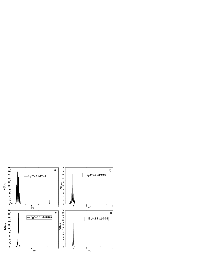
Figure 1: The spectral function of the two-site Holstein model at $k=0$. When $\omega_{0}/t\to 0$ the spectral function converges to a single $\delta$-function.

In the case when the ground state does not have polarons the solution of Eq.(4) is trivial $\varphi_{\mathbf{n}}=0$. The nonadiabatic correction to the spectral function may be calculated by the standard perturbation theory. The dimensionless parameter, which determines the perturbation series is $g\omega_{0}/2t=\sqrt{\lambda\omega_{0}/2t}\propto(m/M)^{1/4}$. Therefore, the perturbation theory may be considered as an expansion in series over the adiabatic parameter $(m/M)^{1/2}$ because the expansion contains only even powers of the coupling constant. In order to calculate the spectral function with the given accuracy $\delta$ it is necessary to calculate all irreducible diagrams for the self-energy up to the order $n$ which satisfies the inequality $(g\omega_{0}/2t)^{n}=(\lambda\omega_{0}/2t)^{n/2}<\delta$. If we consider realistic parameters for crystalline materials $\omega_{0}/2t\leq 0.1$ for required accuracy better than $\delta=10$% for $\lambda\leq 3$ we have to take into account fourth order diagrams for the self-energy. Indeed, $\lambda^{2}(\omega_{0}/2t)^{2}\leq 0.09<0.1$.

Nevertheless, in the 1D Holstein model, the self-energy diverges near the threshold of the phonon emission. This divergence becomes even more pronounced in higher orders of the perturbation theory. It is easy to see by the comparison of the contribution of the second-order and the fourth-order diagrams for the self-energy. The second order contribution diverges near the threshold as $|x|^{-1/2}$ while the fourth order contribution diverges as $|x|^{-3/2}$, here $x=1-(\epsilon-\omega_{0})/2t$ describes the deviation from the threshold. It demonstrates that in order to describe the behaviour of the self-energy correctly the summation of all diagrams which contain the same divergencies should be performed LevinsonRashba ; Pitaevskii .

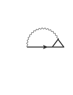
Figure 2: Diagrammatic representation of Dyson equation with renormalized vertex.

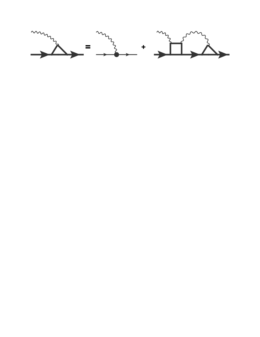
Figure 3: Diagrammatic representation of the integral equation for the vertex. The kernel of the equation is defined by the square with two external electronic lines and with two external phonon lines.

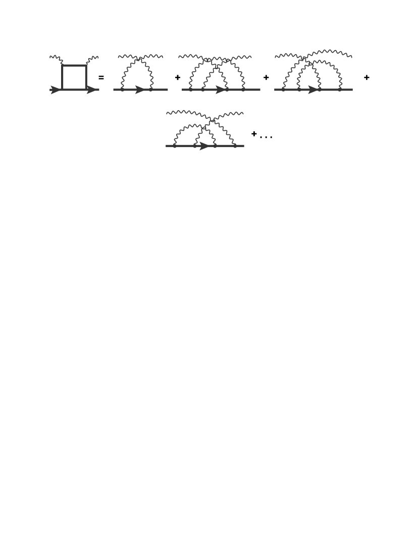
Figure 4: Diagrammatic representation of the perturbation expansion for the square. This expansion is exact up to the sixth order in perturbation theory and correctly accounting for the threshold effects.

Following the procedure LevinsonRashba ; Pitaevskii we formulate Dyson’s equation for the electron self-energy $\Sigma(\epsilon,k)$ (Fig.(2) where the vertex part $\Gamma(\epsilon,k,q)$ satisfies the equation schematically represented in Fig.(3). The kernel $K(\epsilon,k,q,x)$ of the integral equation for the vertex part $\Gamma(\epsilon,k,q)$ is represented by the square, which contains all irreducible diagrams with one incoming and one outcoming electron lines and one incoming and one outcoming phonon lines. The kernel may be evaluated by perturbation theory, schematically represented in Fig.(4). If we sum all diagrams contributing to this kernel we present the exact solution of the problem with $\varphi_{\mathbf{n}}=0$. The exponentially small terms corresponding to the overlap of the states with and without deformation cannot be evaluated in this procedure because of the non-analytic nature of these terms. The diagrams shown in Fig.(4) allow evaluating vertex (Fig.(3) which is exact in sixth order of perturbation expansion and correctly describes the threshold effects. Finally, the solution of Dyson’s equation (Fig.(2)) with the vertex defined by Fig.(3) and with the kernel defined by diagrams, plotted in Fig.(4) represents the summation of all diagrams, where the number of crossings in each phonon line is less than four. This theory is accurate up to the sixth order in the dimensionless parameter $(\lambda\omega_{0}/2t)^{1/2}\propto(m/M)^{1/4}$ and correctly describes the behaviour of the self-energy near the phonon emission threshold. Therefore, the accuracy of our calculations for $\lambda<3$ and $\omega_{0}\leq 0.2t$ is better than 3%.

After integration over energies Dyson’s equation represented in Fig.(2) and the equation for the vertex part represented in Fig.(3) have the form:

$$\Sigma(\epsilon,k)={g\omega_{0}\over{2\pi}}\int_{-\pi}^{\pi}\Gamma(\epsilon,k,q)G(\epsilon-\omega_{0},k-q)dq,$$ (13)

and

$$\Gamma(\epsilon,k,q)=g\omega_{0}+\int_{-\pi}^{\pi}K(\epsilon,k,q,x)G(\epsilon-\omega_{0},k-x)\Gamma(\epsilon,k,x){dx\over{2\pi}}.$$ (14)

The kernel $K(\epsilon,k,q,x)$ calculated up to the sixth order in perturbation theory (Fig.(4)) is represented by the equation:

$$K(\epsilon,k,q,x)=(g\omega_{0})^{2}G(\epsilon-2\omega_{0},k-q-x)+(g\omega_{0})^{4}\int_{-\pi}^{\pi}G(\epsilon-3\omega_{0},k-q-x-y)\times\Bigl{(}$$

$$G(\epsilon-2\omega_{0},k-q-y)G(\epsilon-2\omega_{0},k-x-y)+G(\epsilon-2\omega_{0},k-q-x)G(\epsilon-2\omega_{0},k-x-y)+$$

$$G(\epsilon-2\omega_{0},k-q-y)G(\epsilon-2\omega_{0},k-q-x)\Bigr{)}{dy\over{2\pi}}.$$ (15)

Here the electron Green’s function is defined as:

$$G(\epsilon,k)={1\over{\epsilon+2t\cos{(k)}-\Sigma(\epsilon,k)}}.$$ (16)

As a result, the problem of calculation of the spectral function is reduced to a solution of two integral equations for the self-energy Eq.(13) and for the vertex part Eq.(14) with the kernel, defined by Eq.(15). Here we present the numerical solution to these equations. We also propose an accurate approximation for the vertex part and compare the numerical solution with the approximate solution.

In order to solve Eqs.(13,14) the energy was defined in 3001 points on the interval $-6t<\epsilon<6t$. The momentum was defined in 101 points of the Brillouin zone $-\pi<k<\pi$ with the step $\Delta h=2\pi/100$. The integration was performed by the trapezoidal rule with the accuracy $\sim(\Delta h)^{2}$ better than 1%. As a staring point of the iteration procedure, we introduce the vertex and the self-energy which are averaged over momenta and represent the solution of Eqs.(13,14) averaged over momenta

$$\Gamma_{av}(\epsilon)=g\omega_{0}/\Bigl{[}1-{{g^{2}\omega_{0}^{2}\over{t^{2}}}(1+{{g^{2}\omega_{0}^{2}\over{t^{2}}}\over{[(z_{2}-z_{2}^{-1})(z_{3}-z_{3}^{-1})]}})\over{[(z_{1}-z_{1}^{-1})(z_{2}-z_{2}^{-1})]}}\Bigr{]}.$$ (17)

Here $z_{n}$ is the smallest ($|z_{n}|\leq 1$) root of the quadratic equation $z^{2}+\epsilon_{n}/tz+1=0$, and $\epsilon_{n}=\epsilon-n\omega_{0}-\Sigma(\epsilon-n\omega_{0})$. The self-energy $\Sigma(\epsilon)$ is defined from Eq.(13) with approximate vertex $\Gamma_{av}(\epsilon)$. Note, that the Green’s function Eq.(16) with this self-energy satisfies the sum rules up to the seventh order.

The approximate self-energy and vertex part are used as a starting point to solve Eqs.(13,14) iteratively. The iteration procedure looks as follows. On every step the self-energy is calculated from Eq.(13) with the vertex from the previous step. Then the new self-energy is used to obtain the new vertex from Eq. (14). Dyson’s equation Eq. (13) was solved by iterations. On the other hand, the standard routine for the solution of the system of the linear equation from the NAG library was used in every step of the iteration. Usually, only a few iterations are necessary to obtain solutions for the vertex part and the self-energy Eqs.(13,14). The results of calculations are presented in Fig(5a).

To construct an approximate solution for the vertex $\Gamma(\epsilon,k,q)$ we notice first, that the main contribution to the integral in Eq.(14) comes from the vicinity of $x=k$ point. Note, that $k-x=0$ point represents the Van Hove singularity in Eq. (14), because at this point group velocity is equal to 0. Therefore, we may take out the vertex part $\Gamma(\epsilon,k,k)$ from the integral. As a result, we obtain:

$$\Gamma_{app}(\epsilon,k,q)=g\omega_{0}+\Gamma_{app}(\epsilon,k,k)F(\epsilon,k,q),$$ (18)

where $F(\epsilon,k,q)=\int_{-\pi}^{\pi}K(\epsilon,k,q,x)G(\epsilon-\omega_{0},k-x){dx\over{2\pi}}$ Rewriting this equation at $q=k$ and then solving equation for $\Gamma(\epsilon,k,k)$, we obtain approximation for the vertex:

$$\Gamma_{app}(\epsilon,k,q)=g\omega_{0}+g\omega_{0}F(\epsilon,k,q)/(1-F(\epsilon,k,k)).$$ (19)

Integrals in formula for $F(\epsilon,k,q)$ may be calculated analytically (See Appendix A). Substituting this vertex with analytic formulae for $F(\epsilon,k,q)$ Eqs.(29,30,31,32) to Dyson equation Eq.(13) we calculate spectral function, presented in Fig.(5b). Comparison of spectral functions presented in Fig.(5a) and Fig.(5b) demonstrates that indeed the main contribution to the vertex $\Gamma(\epsilon,k,q)$ is coming from the vicinity of the Van Hove singularity in Eq.(14). Therefore, there is very good agreement between numerical solution of Eqs.(13,14,15) and approximate results for the spectral function. Note, that both spectral functions satisfy the sum rules up to the seventh moment (Fig(6)).

Fig.(5) clearly demonstrates that the lowest energy band has minimum at $\epsilon=\epsilon(k=0)\propto(E^{2}_{p}\omega^{2}_{0}/t)^{1/3}\sim(m/M)^{1/3}$. With increasing $k$ the energy disperses relatively quick up to the energy of the order of $\epsilon(k)=\epsilon(k=0)+\omega_{0}$ at $k\approx\sqrt{2m\omega_{0}}$ and then remains unchanged with further increase of $k$ up to the Brillouin zone edge. This effect is well known in literature LevinsonRashba and called the threshold phenomenon. Note that the threshold phenomena were first discussed in connection with the excitation spectrum of the superfluid $He$ by Pitaevskii Pitaevskii . In the case of the 1D Holstein model, the anomaly in the self-energy belongs to type ”c” as discussed by Levinson and Rashba LevinsonRashba and more recently by Goodvin and Beciu Goodvin2010 . The self-energy shows a strong divergence $-(-2t+\omega_{0}-\epsilon)^{-1/2}$ when $\epsilon\to-2t+\omega_{0}-0$. This first branch of the spectrum does not have any damping, because any inelastic scattering of electrons is forbidden by the conservation of energy. The anomalies similar to the threshold effect are also present at higher energies because the higher order diagrams have additional divergence at $-2t+n\omega_{0}$, $n=1,2,3,...$. These anomalies are much less pronounced because of the finite imaginary part of the self-energy at these energies. And finally, there is an increase of $A(k,\omega)$ near $ka=\pi$ and $\omega>2t$. This peak is less pronounced than the peak at the bottom of the band, because it has finite damping.

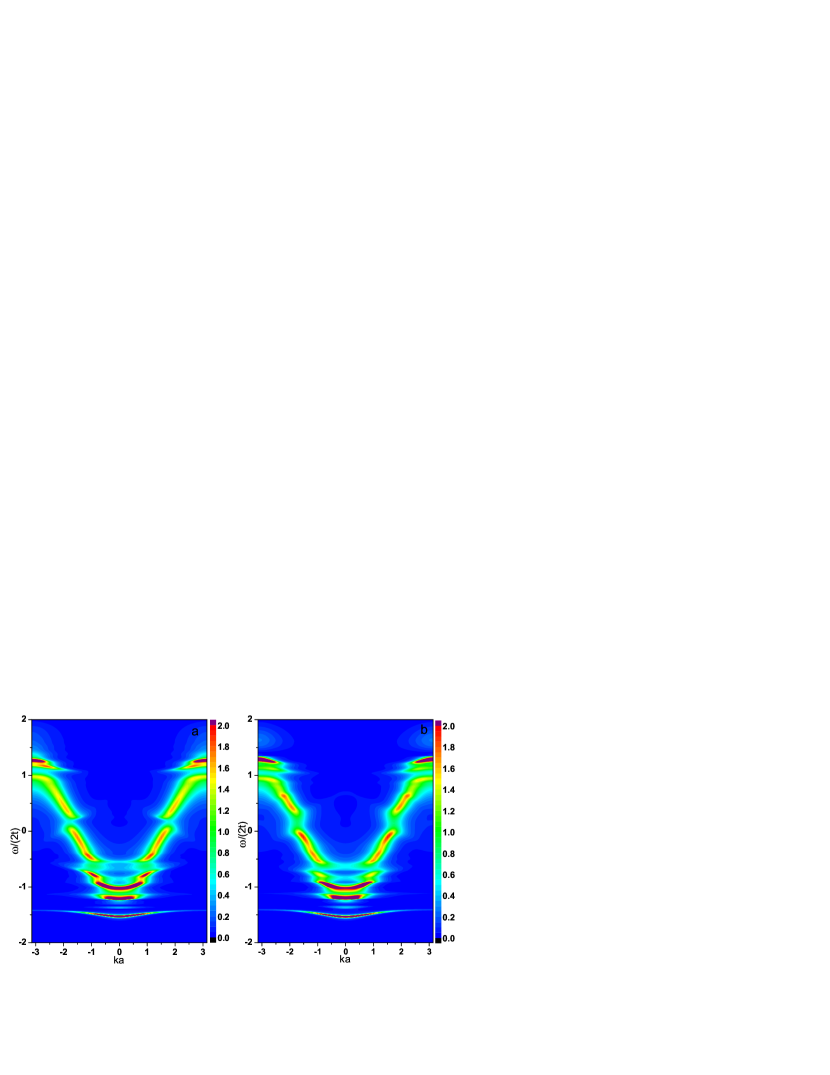
Figure 5: 2D plot of the spectral function of the 1D Holstein model in the limit $\mu\to-\infty$. $E_{p}/2t=2.5$ and $\omega/2t=0.1$. Colors represent the value of the spectral function at given energy and momentum. Exact numerical solution of Eqs.(13,14) (a), and approximation Eq.(19) for the vertex part (b).

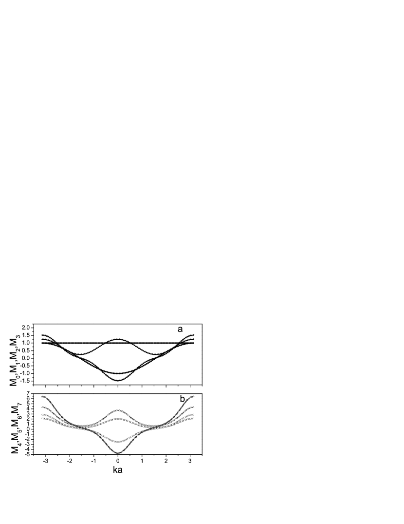
Figure 6: Moments of the spectral function calculated numerically (symbols) in comparison with exact sum rules (lines) for a) $M_{0}$ full squares, $M_{1}$ full circles, $M_{2}$ full triangles, $M_{3}$ full stars, b) $M_{4}$ empty squares, $M_{5}$ empty circles, $M_{6}$ empty triangles, and $M_{7}$ empty stars.

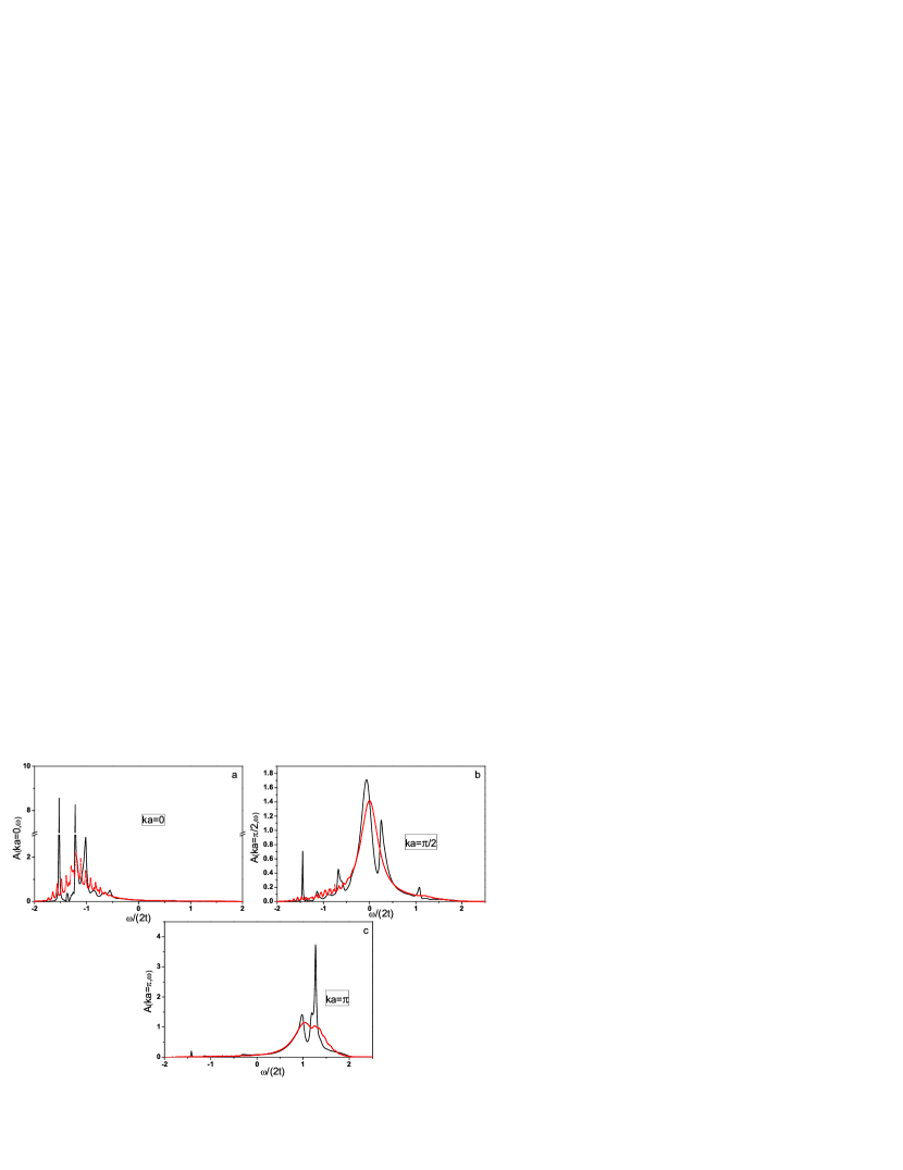
Figure 7: The spectral function of the 1D Holstein model in the limit $\mu\to-\infty$ at different points of the Brillouin zone. Dotted lines represent the spectral function calculated within the momentum averaged approximation with corrections of level two. $E_{p}/2t=2.5$ and $\omega/2t=0.1$.

Now let us compare the present theory, which takes into account all diagrams up to the sixth order and represents the partial summation of infinite perturbation series with the momentum average approximation, proposed in Ref.(Berciu ). This theory is accurate in the second-order approximation. The fourth-order contribution in this theory is approximated by the self-energy contribution:

$$\Sigma_{4}(k,\epsilon)\approx 2{g^{4}\omega_{0}^{4}\over{(2t)^{3}}}I^{2}(z_{1})I(z_{2}),$$ (20)

which is equal to an averaged over $k$ fourth order diagram with phonon lines crossings (22), and $I(z)=2/(z-z^{-1})$. This expression should be compared with the exact forth order contribution $\Sigma_{4}(k,\epsilon)=\Sigma_{4}^{NC}(k,\epsilon)+\Sigma_{4}^{C}(k,\epsilon)$, where

$$\Sigma_{4}^{NC}(k,\epsilon)=4{g^{4}\omega_{0}^{4}\over{(2t)^{3}}}{z_{1}+1/z_{1}\over{(z_{1}-1/z_{1})^{3}}}I(z_{2}),$$ (21)

$$\Sigma_{4}^{C}(k,\epsilon)={g^{4}\omega_{0}^{4}\over{(2t)^{3}}}{2(1-z_{1}^{4}z_{2}^{2})\over{z_{1}^{4}z_{2}^{2}+1-2z_{1}^{2}z_{2}cos(k)}}I(z_{1})^{2}I(z_{2}),$$ (22)

here $z_{1}$ and $z_{2}$ ($|z_{1,2}|<1$) roots of quadratic equations, defined after Eq.(17) and are calculated with $\Sigma_{B}(\omega)=-i\delta$. Comparing these results we conclude that momentum average approximation is rather poor because it provides the self-energy which is functionally different from the perturbation theory. Therefore, momentum average approximation is accurate only in the second order in coupling constant. There were few attempts to improve this approximation BerciuGoodvin . The first step of corrections leads to the correct expression for fourth order noncrossing diagram $\Sigma_{4}^{NC}(k,\omega)$ Eq.(21) but fails to take into account $k$-dependence of the diagram with crossing of phonon lines $\Sigma_{4}^{C}(k,\epsilon)$. The next and the last level of corrections leads to some infinite system of inhomogeneous equations, which was solved by truncation. This procedure is not well justified because the coefficient in this equation does not fall with the increasing of the system size. Nevertheless, the solution of this system expanding in powers of the coupling constant may be performed analytically and we recover the correct expression for the fourth-order diagrams. Higher order diagrams require the next level of corrections which were not discussed in Ref.BerciuGoodvin . Therefore, we conclude that momentum average approximation with the corrections of levels 1 and 2 is accurate up to the fourth order in perturbation theory.

In Fig.(7) the spectral function is plotted for three different $ka=0,\pi/2,\pi$. In the same graphs, the spectral functions calculated within momentum average approximations with the corrections of level 2 BerciuGoodvin are presented. There is quite good agreement between spectral functions calculated within these approaches at large momenta ($ka=\pi/2,\pi$). At $ka=0$ the incoherent part of the spectrum is also quite similar in both cases. Nevertheless, the present theory shows much sharper peaks. These spectral functions satisfy the sum rules up to 7th moment (Fig(6)).

III.2 The spectral function in the polaron state

In order to describe the spectral function of the system where the ground state of the grand canonical Hamiltonian $H^{{}^{\prime}}$ corresponds to a finite polaron density, we have to tune the chemical potential close to the single polaron level. The requirement is that the lowest energy state of the grand canonical Hamiltonian $H^{{}^{\prime}}$ with at least one polaron should be lower than the lowest energy level of the Hamiltonian without polarons. In order to prevent bipolaron formation, we consider the spinless fermions and assume that bipolarons represent an excited state on the grand canonical Hamiltonian when the chemical potential is pinned near the polaron level.

The spectral function Eq. (11) has two terms. The first term describes the creation of an additional carrier in the ground state of the grand canonical Hamiltonian $H^{{}^{\prime}}$ with one polaron which is proportional to $1-n$, where $n=1/N$ is the polaron density. More important is the second term which describes the emission of the electron from the ground state which is proportional to $n=1/N$. Importantly, exactly this term is measured in direct photoemission spectroscopy. Note that the second term carries information about polaron formation. This was pointed out in Ref.Pasha3 where the exact formula for the first moment of the spectral function was derived. This first moment has the contribution, which is proportional to the adiabatic polaron shift $2nE_{p}$. Therefore, this term may be derived from the adiabatic theory without involving nonadiabatic corrections.

In the adiabatic approximation, the polaron state is the self-trapped state localized in the translation symmetry broken deformation field $\varphi_{\mathbf{n}}$. This state is degenerate because the polaron energy does not depend on the polaron position and is described by the solution of Eq.(5) $\psi_{\mathbf{n}}^{0}$ with the lowest energy $E_{0}$. Within the sudden approximation the second term in Eq.(11) is proportional to the square of the Fourier transform of the $F_{k}=\sum_{n}\exp{(ikn)}\psi_{\mathbf{n}}^{0}/\sqrt{N}$. Therefore, Eq.(11) is given by a single $\delta$ function:

$$A_{-}({\mathbf{k}},\omega) = 2\pi\sum_{l}|\langle l|c_{\mathbf{k}}|0\rangle|^{2}\delta(\omega+{\cal E}_{l}-{\cal E}_{0})$$ (23)

$$= 2\pi|F_{k}|^{2}\delta(\omega-E_{0}+\mu).$$

Since the polaron wave function is localized $F_{k}\propto 1/N^{1/2}$ the spectral function $A_{-}(k,\omega)$ is proportional to polaron density $N^{-1}$ (one polaron per $N$ sites). The chemical potential $\mu$ is pinned to the polaron energy $\mu=E_{0}+E_{p}\sum_{n}|\psi_{n}^{0}|^{4}$ Kabanov which is the sum of the lowest eigenvalue of Eq(5) and the deformation energy caused by the polaron. In the strong coupling limit $\mu=-E_{p}-t^{2}/E_{p}$ therefore the peak of the spectral function $A(k,\omega)$ is at energy $\omega=-E_{p}+t^{2}/E_{p}$. Note, that the spectral function is equal to 0 at the chemical potential ($\omega=0$). This is because the overlap of the wave functions with and without polaron deformation is exponentially small and the annihilation of the polaron together with the deformation is forbidden due to the Franck-Condon principle. The part of the spectral function associated with the inverse photo-emission is given by the first part of Eq.(11) and may be written as

$$A_{+}({\mathbf{k}},\omega) = 2\pi\sum_{n}|\langle n|c_{\mathbf{k}}^{\dagger}|0\rangle|^{2}\delta(\omega+{\cal E}_{0}-{\cal E}_{n})$$ (24)

$$= 2\pi\sum_{l\neq 0}|F_{k}^{l}|^{2}\delta(\omega-E_{l}+\mu),$$

where $F_{k}^{l}=\sum_{n}\exp{(ikn)}\psi_{\mathbf{n}}^{l}/\sqrt{N}$ is the Fourier transform of the wave function which represents the $l$-th eigenstate of Eq.(3) where $\varphi_{\mathbf{n}}$ is determined by Eq.(4) with $\psi_{\mathbf{n}}^{l}=\psi_{\mathbf{n}}^{0}$. Here the sum does not include $l=0$ because the absorption of electron directly to the polaronic state is proportional to the overlap of the lattice wave functions with zero and nonzero deformation which is exponentially small $\propto\exp{(-\sqrt{M/m})}$. As in the photoemission case this process is forbidden due to the Franck-Condon principle. Note that the spectrum has a clear pseudogap, which corresponds to $|E_{0}|-2t\approx 2E_{p}-2t$. The physics of this pseudogap is simple. The probability to remove polaron from the Fermi level or the probability to add polaron to the Fermi level is exponentially suppressed and these processes are too weak to observe them experimentally. Therefore, the main features of the spectral function are shifted from the Fermi energy because of the Franck-Condon principle.

In Fig.(8) the spectral function of the polaron is plotted for the 1D system with 100 sites with periodic boundary conditions in the adiabatic limit for the polaron binding energy $E_{p}=2.5t$ Fig.(8a) and for $E_{p}=0.5t$ Fig.(8b). The main spectral features repeat the free electron spectrum except that the presence of polaron deformation breaks the translation invariance. Therefore, the linewidth has finite broadening due to the scattering of a free electron on the polaron deformation. As expected, this spectral density satisfies the zero $M_{0}=1$ and the first $M_{1}=-2tcos(ka)-2nE_{p}$ sum rules, $a$ is the lattice constant and $n=1/N$ is the polaron density.

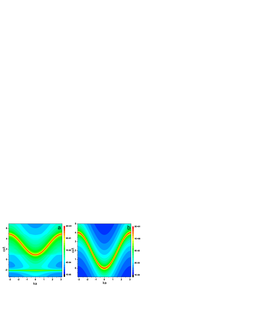
Figure 8: 2D plot of the polaron spectral function in the adiabatic limit for 1D chain with $N=100$ and periodic boundary conditions. Polaron density is therefore $n=0.01$. Colors represent the value of the spectral function at given energy and momentum. a) $E_{p}=2.5t$, $E_{0}=-4.9808t$ and $\mu$ is pinned by polaron level at $-2.9087t$. b) $E_{p}=0.5t$, $E_{0}=-2.0633t$ and the chemical potential $\mu=-2.0210t$.

In the limit when the polaron size is larger than the lattice constant Eqs.(3,4,5) have analytic solutions for both the localized and itinerant part of the spectrum (See Appendix B). Using these solutions the matrix elements $F_{k}$ and $F_{k}^{l}$ in Eqs.(23,24) may be evaluated analytically:

$$F_{k}=\pi\sqrt{t\over{E_{p}N}}{1\over{\cosh{(\pi kat/E_{p})}}},$$ (25)

$$F_{k}^{l} = i(({2lat\over{E_{p}}})^{2}+1-{4t\over{NE_{p}}})^{-1/2}$$ (26)

$$\Bigl{[}-({4lat\over{E_{p}}}){\sin{(\kappa aN/2)}\over{\kappa aN}}+{4\sin^{2}{(\kappa aN/4)}\over{\kappa aN}}+$$

$$- {2\over{\kappa aN}}+{2\pi t\over{E_{p}N}}{1\over{sinh{(\pi\kappa at/E_{p})}}}\Bigr{]}.$$

Here $a$ is the lattice constant, $N$ is the number of sites in the system, $\kappa=l-k$, where $l$ represents the solutions of Eq.(38) $k=2\pi n/Na$ where $n=0,1,2,.,N-1$. These two expressions substituted to Eqs.(23,24) with $E_{0}=-2t-E_{p}^{2}/4t$, $E_{l}=-2t+tl^{2}a^{2}$, and the chemical potential $\mu=-2t-E_{p}^{2}/12t$ provides the analytic description of the spectral function which is accurate up to the nonadiabatic corrections which are small as $\sqrt{m/M}$. Note that this analytic expression satisfies the exact sum rules (i.e. $M_{0}$ and $M_{1}$)Pasha3 when the polaron density is finite.

The spectral function $A(k,\omega)$ calculated on the basis of Eqs.(24,23) using Eqs.(25,26) for two different momenta is plotted in Fig.9. As expected the results are very similar to that plotted in Fig.8. There is a weak spectral intensity at $E_{0}-\mu$. This intensity is proportional to the polaron density and is suppressed quickly when momentum moves away from the $k=0$ point. Main intensity is centered at $\omega=E_{p}^{2}/12t+tk^{2}a^{2}$. Because the exact wave functions Eq.(37) are not plane waves there is a natural broadening of the spectral line due to the scattering of an electron on the polaron deformation. Therefore, the line, corresponding to an almost free electron has finite width in energy. This broadening is very important because it compensates the contribution from the polaron state at negative energies in the sum rules. Therefore, the exact sum rules $M_{0}=1$ and $M_{1}=-2nE_{p}+tk^{2}a^{2}+E_{p}^{2}/12t$ Pasha3 are satisfied.

Note that in Ref. (Pasha3 ) the sum rule $M_{2}$ for the spectral function was derived (See Eq.(15) in Pasha3 ). This moment contains averages of $\langle\varphi_{n}\rangle$ and $\langle\varphi_{n}^{2}\rangle$, which cannot be evaluated exactly. Nevertheless, within the adiabatic approximation, these averages may be easily evaluated. Indeed, Eq.(4), defines the deformation field at site $\mathbf{n}$. Therefore, integration of this equation with $\psi^{0}(x)$ defined by Eq.(34) leads to the result, obtained in Pasha3 $\langle\varphi\rangle=-\sqrt{2}g$ which corresponds to the case of one polaron per $N$ sites. This immediately leads to the correct equation for the momentum $M_{1}$. Similarly, $\langle\varphi^{2}\rangle=2g^{2}\sum_{n}|\psi_{n}^{0}|^{4}$. Calculation of the sum leads to the following result $\langle\varphi^{2}\rangle=g^{2}E_{p}/3t$ in the weak coupling case $E_{p}<<t$ and $\langle\varphi^{2}\rangle=g^{2}(1-t^{2}/E_{p}^{2})$. Therefore, the second moment of the spectral function has the form:

$$M_{2}=(\epsilon(k)-\mu)^{2}-4nE_{p}(\epsilon(k)-\mu)+\begin{cases}2nE_{p}^{3}/3t&\textrm{if $E_{p}<<t$}\\ 4n(E_{p}^{2}-t^{2})&\textrm{if $E_{p}>>t$}\end{cases}+{\cal O}(\sqrt{m/M}).$$ (27)

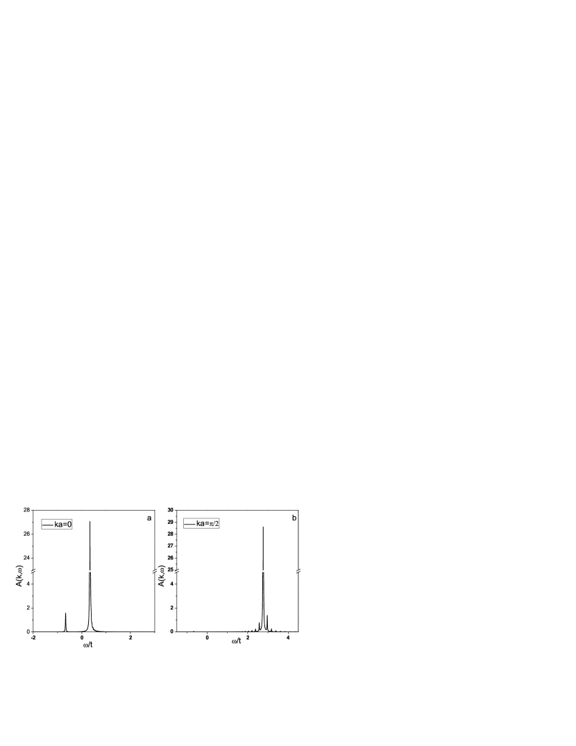
Figure 9: The polaron spectral function in the adiabatic limit for the 1D chain with $N=100$ in the continuous limit and the polaron density $n=0.01$. $E_{p}=2t$ and the chemical potential $\mu=-2t-t/3$ and the polaron binding energy $E_{0}=-3t$ a) $ka=0$. b) $ka=\pi/2$.

In Fig.10 the calculated sum rule $M_{2}$ is plotted as a function of momentum $k$ in comparison with expression Eq.(27). The calculations are performed for the tight binding model (Eq.(3,4)) and for analytic differential equation (35). In both cases the results perfectly match the analytic formula Eq.(27).

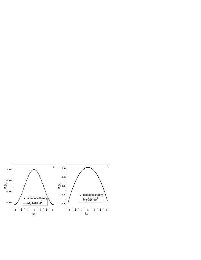
Figure 10: The second moment of the spectral function as a function of the momentum $k$ calculated in the adiabatic limit. a) Tight binding calculations with $E_{p}=0.4t$ and $\mu=-2.0134t$. b) Analytic solution of Eq.(35) with $E_{p}=2t$ and $\mu=-2.3333t$.

IV Conclusion

We formulate the analytic theory for the spectral function of the electron-phonon system in the adiabatic limit. In the limit of the dilute polaron system where the polaron density $n\to 0$ and when the chemical potential is large and negative $\mu\to-\infty$ the polaron deformation is absent and the spectrum of electrons coupled to phonons is defined by the standard perturbation theory. Using the diagram technique with an accurate account of threshold effects we were able to formulate an integral equation for the vertex, which takes into account all diagrams up to the sixth order. Then we solve Dyson’s equation for the self-energy with the renormalized vertex and calculate the polaron spectral function in 1D with an accuracy better than 3% for $\lambda\leq 3$ in the adiabatic limit. The moments of the spectral function satisfy the exact sum rules up to the 7th moment.

For the system with a finite polaron density when the chemical potential is pinned at the polaron level the ground state has nonzero adiabatic deformation due to the presence of polarons. In this case, the spectral function is calculated in the adiabatic limit without any non-adiabatic corrections. We also show how the adiabatic terms, proportional to the polaron density $n$, may be evaluated for higher-order moments. The spectral function shows weak spectral intensity at $E_{0}-\mu$, which is proportional to $n$. At the Fermi level in the adiabatic limit the spectral density is absent. Continuous spectrum starts at $-\mu-2t>0$. Therefore, the spectrum has a gap, which is proportional to the polaron binding energy $E_{0}$. Contrary to the case of $n=0$ the spectral function with a finite polaron density has some adiabatic contributions which are characteristic of the polaron formation.

V ACKNOWLEDGMENTS

The author thanks D. Mihailovic, T. Mertelj and especially P.E. Kornilovitch for very helpful and enlightening discussions and acknowledges the financial support from the Slovenian Research Agency Program No. P1-0040.

Appendix A Appendix A

A.1 Derivation of analytical formula for approximate vertex.

The integrals in the expression for function $F(\epsilon,k,q)$ may be evaluated analytically. After the substitution $z=\exp{(ik)}$ the integral becomes $\int_{-\pi}^{\pi}dk/2\pi\to\oint_{|z|=1}dz/2i\pi z$ and is determined by the poles of the integrand within the unite circle $|z|=1$. The residues are determined by the quadratic equation: $z^{2}-\epsilon_{n}z/t+1=0$, which has two roots $z_{n}$ ($|z_{n}|\leq 1$) and $1/z_{n}$. Therefore, all integrals for $F(\epsilon,k,q)$ are expressed in terms of $z_{n}$. Here $\epsilon_{n}=\epsilon-n\omega_{0}-\Sigma(\epsilon-n\omega_{0})$ and $\Sigma(\epsilon)$ is the solution of Dyson equation (13) determined with $\Gamma_{av}(\epsilon)$ Eq.(17).

$$F(\epsilon,k,q) = F_{2}(\epsilon,k,q)+F_{4,1}(\epsilon,k,q)+$$ (28)

$$F_{4,2}(\epsilon,k,q)+F_{4,3}(\epsilon,k,q),$$

where $F_{2}$ represents second order contribution, and $F_{4,i}$, $i=1,2,3$ represent three contributions of forth order in accordance with Eq.(15)

The second-order contribution has the form:

$$F_{2}(\epsilon,k,q)={4g^{2}\omega_{0}^{2}\over{(z_{1}-z_{1}^{-1})(z_{2}-z_{2}^{-1})}}\Big{[}{z_{1}z_{2}\over{\mu-z_{1}z_{2}}}-{z_{1}^{-1}z_{2}^{-1}\over{\mu-z_{1}^{-1}z_{2}^{-1}}}\Big{]}.$$ (29)

Three fourth order terms after cumbersome calculations have the following form:

$$F_{3,1}(\epsilon,k,q) = {16g^{4}\omega_{0}^{4}\over{(z_{1}-z_{1}^{-1})(z_{2}-z_{2}^{-1})^{2}(z_{3}-z_{3}^{-1})}}\Big{[}{\eta z_{2}z_{3}\over{\mu-z_{2}z_{3}}}\big{(}{z_{1}z_{2}^{2}\over{\mu-\eta z_{1}z_{2}^{2}}}+{1\over{\eta-z_{1}z_{2}z_{3}}}\big{)}+{\eta z_{1}z_{2}z_{3}\over{(\eta-z_{1}z_{2}z_{3})(\eta-\mu z_{1}z_{2}^{2})}}$$ (30)

$$+{\eta z_{2}^{-1}z_{3}^{-1}\over{\mu-z_{2}^{-1}z_{3}^{-1}}}\big{(}{z_{1}^{-1}z_{2}^{-2}\over{\mu-\eta z_{1}^{-1}z_{2}^{-2}}}+{1\over{\eta-z_{1}^{-1}z_{2}^{-1}z_{3}^{-1}}}\big{)}+{\eta z_{1}^{-1}z_{2}^{-1}z_{3}^{-1}\over{(\eta-z_{1}^{-1}z_{2}^{-1}z_{3}^{-1})(\eta-\mu z_{1}^{-1}z_{2}^{-2})}}\Big{]},$$

$$F_{3,2}(\epsilon,k,q) = {16g^{4}\omega_{0}^{4}\over{(z_{1}-z_{1}^{-1})(z_{2}-z_{2}^{-1})^{2}(z_{3}-z_{3}^{-1})}}\Big{[}{z_{1}z_{2}z_{3}\over{\eta-z_{1}z_{2}z_{3}}}\big{(}{z_{1}z_{2}\over{\mu-z_{1}z_{2}}}+{\eta\over{\eta-\mu z_{2}^{2}z_{3}}}\big{)}+{\mu z_{1}z_{2}\over{(\mu-z_{1}z_{2})(\mu-\eta z_{2}^{2}z_{3})}}$$ (31)

$$+{z_{1}^{-1}z_{2}^{-1}z_{3}^{-1}\over{\eta-z_{1}^{-1}z_{2}^{-1}z_{3}^{-1}}}\big{(}{z_{1}^{-1}z_{2}^{-1}\over{\mu-z_{1}^{-1}z_{2}^{-1}}}+{\eta\over{\eta-\mu z_{2}^{-2}z_{3}^{-1}}}\big{)}+{\mu z_{1}^{-1}z_{2}^{-1}\over{(\mu-z_{1}^{-1}z_{2}^{-1})(\mu-\eta z_{2}^{-2}z_{3}^{-1})}}\Big{]},$$

$$F_{3,3}(\epsilon,k,q) = {16g^{4}\omega_{0}^{4}\over{(z_{1}-z_{1}^{-1})(z_{2}-z_{2}^{-1})^{2}(z_{3}-z_{3}^{-1})}}\big{[}{z_{2}z_{3}\over{\mu-z_{2}z_{3}}}-{z_{2}^{-1}z_{3}^{-1}\over{\mu-z_{2}^{-1}z_{3}^{-1}}}\big{]}\big{[}{z_{1}z_{2}\over{\mu-z_{1}z_{2}}}-{z_{1}^{-1}z_{2}^{-1}\over{\mu-z_{1}^{-1}z_{2}^{-1}}}\big{]}.$$ (32)

Here $\mu=\exp{(iq)}$ and $\eta=\exp{(ik)}$.

Appendix B Appendix B

B.1 Derivation of the spectral function in the continuous limit.

Eq.(5) in 1D in the weak coupling limit $t>>E_{p}$ when the polaron radius is much larger than the lattice constant has an analytic solution. In that limit Eq.(5) may be rewritten in a differential form. Indeed, expanding $\psi_{\mathbf{n+m}}$ in a Taylor series up to the second order in the lattice constant Eq.(5) has the form:

$$-ta^{2}{d^{2}\psi(x)\over{dx^{2}}}-2E_{p}|\psi(x)|^{2}\psi(x)=(E+2t)\psi(x).$$ (33)

It is easy to check that the function

$$\psi^{0}(x)=({E_{p}\over{4t}})^{1/2}{1\over{\cosh{(E_{p}x/2at)}}}$$ (34)

is the solution of Eq.(33) corresponding to the bound state energy $E_{0}=-2t-E_{p}^{2}/4t$. Therefore, Eq.(3) with deformation field $\varphi^{0}(x)$ from Eq.(4) may be rewritten as:

$$-ta^{2}{d^{2}\psi(x)\over{dx^{2}}}-{E_{p}^{2}\over{2t}}{\psi(x)\over{\cosh^{2}{(E_{p}x/2at)}}}=(E+2t)\psi(x).$$ (35)

Rescaling the spatial variable $E_{p}x/2at\to x$ this equation is reduced to the well known equation KabanovAlexandrov2008 :

$$-{d^{2}\psi(x)\over{dx^{2}}}-{2\psi(x)\over{\cosh^{2}{(x)}}}=\epsilon\psi(x).$$ (36)

This equation is integrable and has analytic eigenfunctions. Therefore, the excited states of Eq.(35) have the following form:

$$\psi(x)=\Bigl{(}{2ikat\over{E_{p}}}-\tanh{({E_{p}x\over{2at}})}\Bigr{)}\exp{(ikx)}$$ (37)

with the excited state energies $E_{k}=-2t+tk^{2}a^{2}$. These wave functions satisfy the periodic boundary conditions when

$$ka\tan{(kL/2)}+{E_{p}\over{2t}}tanh{({E_{p}L\over{4ta}})}=0,$$ (38)

where $L=Na$. This equation has $N-1$ roots for corresponding to $N-1$ itinerant states, because one state splits to localised polaron level $E_{0}$. These values of $k$ together with $\psi^{0}(x)$ (Eq.(34)) define the complete set of eigenfunctions of Eq.(35). The Fourier transform of these eigenfunctions defines the matrix elements Eqs.(25,26) which determine the polaron spectral function.

References

- (1) I. G. Austin, N. F. Mott, Advances in Physics, 18, 41 (1969).
- (2) S.R. Elliott, Advances in Physics, 36, 135 (1987).
- (3) A.S. Alexandrov, N.F. Mott, Rep. Prog. Phys. 57, 1197 (1994).
- (4) A.S. Alexandrov, A.B. Krebs, Sov. Phys. Usp. 35, 345 (1992).
- (5) A.S Mishchenko, Sov. Phys. Usp. 48, 887 (2005).
- (6) J. T. Devreese, A. S. Alexandrov, Rep. Prog. Phys. 72, 066501 (2009).
- (7) M.I. Klinger, Sov. Phys. Usp. 28, 391 (1985).
- (8) S.I. Pekar, Research in Electron Theory of Crystals, AEC-tr-555, US Atomic Energy Commission (1963).
- (9) G.C. Kuper, G.D. Whitfield, eds. ”Polarons and Excitons”. Oliver and Boyd, Edinburgh (1963).
- (10) J. Appel ”Polarons”. In: Solid State Physics, F. Seitz, D. Turnbull, and H. Ehrenreich (eds.), Academic Press, New York. 21, 193 (1968).
- (11) A.S. Alexandrov, J.T. Devreese, Advances in Polaron Physics, Springer Series in Solid-State physics. 159. Heidelberg: Springer-Verlag.
- (12) A.S. Alexandrov, N. Mott, ”Polarons and Bipolarons”. World Scientific, Singapore (1996).
- (13) D.Emin, Polarons, Cambridge University Press, Cambridge (2013).
- (14) V. Coropceanu, J. Cornil, D.A. da Silva Filho, Y. Olivier, R. Silbey, and J.-L. Bredas, Chem. Rev. 107, 926, (2007); J.-L. Bredas, D. Beljonne, V. Coropceanu, J. Cornil, Chem. Rev. 104, 4971, (2004).
- (15) R. Zamboni, A.J. Pal, C. Taliani, Solid State Commun. 70, 813 (1989); C. Taliani, R. Zamboni, G. Ruani, F. C. Mataeotta, K. I. Pokhodnya, Solid State Commun. 66, 487 (1988).
- (16) D. Mihailovic, C.M. Foster, K. Voss, A.J. Heeger, Phys. Rev. B 42, 7989 (1990).
- (17) J.P. Falck, A. Levy, M.A. Kastner, R.J. Birgeneau, Phys. Rev. B 48, 4043 (1993).
- (18) P. Calvani, M. Capizzi, S. Lupi, P. Maselli, A. Paolone, R. Roy, S.W. Cheong, W. Sadowski, E. Walker, Solid State Commun. 91, 113 (1994).
- (19) D.M. Eagles, Phys. Rev. 130, 1381 (1963).
- (20) M.I. Klinger, Phys. Lett., 7, 102 (1963).
- (21) H.G. Reik, Solid State Commun. 1, 67 (1963).
- (22) D. Emin, Phys. Rev. B 48, 13691 (1993).
- (23) A.S. Alexandrov, V.V. Kabanov, D.K. Ray, Physica C 224, 247 (1994).
- (24) T.-H. Höck, H. Nickisch, H. Thomas, Helv. Phys. Acta, 56, 237 (1983).
- (25) Y. Tokura, Colossal Magnetoresistance Oxides, (Gordon and Breach, New York, 2000).
- (26) A.J. Millis, B.I. Shraiman, R. Mueller, Phys. Rev. Lett. 77, 175 (1996); A.J. Millis, R. Mueller, and B.I. Shraiman, Phys. Rev. B 54, 5405 (1996).
- (27) J. Ranninger and U. Thibblin, Phys. Rev. B 45, 7730 (1992).
- (28) A.S. Alexandrov, V.V. Kabanov, D.K. Ray, Phys. Rev. B 49, 9915 (1994).
- (29) J. Bonca, S.A. Trugman, I. Batistic, Phys. Rev. B 60, 1633 (1999).
- (30) G. Wellein, H. Roder, and H. Fehske, Phys. Rev. B 53, 9666 (1996).
- (31) M. Capone, W. Stephan, and M. Grilli, Phys. Rev. B 56, 4484 (1997).
- (32) A. Alvermann, H. Fehske, and S.A. Trugman, Phys. Rev. B 81, 165113 (2010).
- (33) H. De Raedt, A. Lagendijk, Phys. Rev. Lett. 49, 1522 (1982);Phys. Rev. B 27, 6097 (1983).
- (34) P.E. Kornilovitch, E.R. Pike, Phys. Rev. B 55, R8634 (1997).
- (35) P.E. Kornilovitch, Phys. Rev. Lett. 81, 5382 (1998).
- (36) A.S. Mishchenko, N.V. Prokof’ev, A. Sakamoto, B.V. Svistunov, Phys. Rev. B 62, 6317 (2000).
- (37) A.W. Romero, D.W. Brown, and K. Lindenberg, J. Chem. Phys. 109, 6540 (1998).
- (38) E. Jeckelmann, S.R. White, Phys. Rev. B 57, 6376 (1998).
- (39) M.Berciu, Phys. Rev. Lett., 97, 036402 (2006); G.L. Goodvin, M. Berciu, G.A. Sawatzky, Phys. Rev. B 74, 245104 (2006).
- (40) S. Paganelli and S. Ciuchi, J. Phys.: Condens. Matter 18, 7669 (2006).
- (41) A.S. Alexandrov, J. Ranninger, Phys. Rev. B 45, 13109 (1992).
- (42) M. Hohenadler, M. Aichhorn, and W. von der Linden, Phys. Rev. B 68, 184304 (2003).
- (43) G. De Filippis, V. Cataudella, V. Marigliano Ramaglia, and C. A. Perroni, Phys. Rev. B 72, 014307 (2005).
- (44) V. Cataudella, G. De Filippis, A. S. Mishchenko, and N. Nagaosa, Phys. Rev. Lett. 99, 226402 (2007).
- (45) L. Vidmar, J. Bonca, and S.A. Trugman, Phys. Rev. B 82, 104304 (2010).
- (46) G.L. Goodvin and M. Berciu, EPL, 92, 37006 (2010).
- (47) J. Bonca, S. A. Trugman, M. Berciu, Phys. Rev. B 100, 094307 (2019).
- (48) T. Holstein, Annals of Physics, 8, 325 (1959); Annals of Physics, 8, 343 (1959).
- (49) V.V. Kabanov, O.Yu. Mashtakov, Phys. Rev. B 47, 6060 (1993).
- (50) P.E. Kornilovitch, Europhys. Lett. 59, 735 (2002).
- (51) H. Fröhlich, Advances in Physics, 3, 325 (1954).
- (52) J.M. Ziman, Electrons and Phonons, Oxford University Press, (1960).
- (53) G. M. Eliashberg, Sov. Phys. JETP 11, 696 (1960); Sov. Phys. JETP 12, 1000 (1960).
- (54) M.A. Smondyrev Theor. Math. Phys. 68, 653 (1986).
- (55) O.S. Barisic, S. Barisic, Eur. Phys. J. B 54, 1 (2006).
- (56) A.S. Alexandrov, V.V. Kabanov, Phys. Rev. B 54, 3655 (1996).
- (57) R. Rajaraman, Solitons and Instantons: An Introduction in Solitons and Instantons in Quantum Field Theory (North-Holland, Amsterdam, 1982).
- (58) F.V. Kusmartsev, Phys. Rev. Lett. 84, 530 (2000); F.V. Kusmartsev, Phys. Rev. Lett. 84, 5026(E) (2000).
- (59) A.S. Alexandrov, V.V. Kabanov, JETP Lett., 72, 569 (2000).
- (60) D. Emin, T. Holstein, Phys. Rev. Lett., 36, 323 (1976).
- (61) P.E. Kornilovitch, Int. J. Mod. Phys. B, 30, 1650105 (2016).
- (62) V. L. Bonch-Bruevich,S. V. Tyablikov, The Green Function Method in Statistical Mechanics, North Holland Publishing Co (1962).
- (63) A.A. Abrikosov, L.P. Gorkov, I.E. Dzyaloshinski, Methods of Quantum Field Theory in Statistical Physics, Englewood Cliffs, Prentice-Hall (1963).
- (64) G.D. Mahan, Many Particle Physics (Plenum, New York, 1981).
- (65) A.L. Fetter, J.D. Walecka, Quantum Theory of Many-Particle Systems, San Francisco, McGraw-Hill, 1971.
- (66) Y.B. Levinson, E.I. Rashba, Rep. Prog. Phys. 36, 1499 (1973); Sov. Phys. Usp.,16, 892 (1974).
- (67) L.P. Pitaevskii, Sov. Phys. JETP, 36, 830 (1959).
- (68) M. Berciu, G.L. Goodvin, Phys. Rev. B, 76, 165109 (2007).
- (69) V.V. Kabanov, A.S. Alexandrov, Phys. Rev. B, 78, 174514 (2008).