The Case for Retraining of ML Models for IoT Device Identification at the Edge

Abstract.

Internet-of-Things (IoT) devices are known to be the source of many security problems, and as such they would greatly benefit from automated management. This requires robustly identifying devices so that appropriate network security policies can be applied. We address this challenge by exploring how to accurately identify IoT devices based on their network behavior, using resources available at the edge of the network.

In this paper, we compare the accuracy of five different machine learning models (tree-based and neural network-based) for identifying IoT devices by using packet trace data from a large IoT test-bed, showing that all models need to be updated over time to avoid significant degradation in accuracy. In order to effectively update the models, we find that it is necessary to use data gathered from the deployment environment, e.g., the household. We therefore evaluate our approach using hardware resources and data sources representative of those that would be available at the edge of the network, such as in an IoT deployment. We show that updating neural network-based models at the edge is feasible, as they require low computational and memory resources and their structure is amenable to being updated. Our results show that it is possible to achieve device identification and categorization with over 80% and 90% accuracy respectively at the edge.

1. Introduction

Internet-of-Things (IoT) devices are the source of a large number of security threats, particularly in domestic deployments (Alrawi et al., 2019). These devices and their platforms would benefit from active and, in particular, automated management – but automating such tasks requires robustly identifying devices to be able to apply appropriate policies, actions, and updates. In this environment, the natural way of identifying IoT devices is to analyze their network behavior at the home router: devices cannot hide behavior as, by definition, they must interact over the network in order to provide functionality. Performing analyses of network behavior at the home router is robust in terms of privacy, scalability and not relying on dependencies from manufacturer-provided cloud-services. Furthermore, there is already nascent support for summarizing such analyses’ results via the MUD standard (Lear et al., 2019). As such, several use cases for IoT device identification arise, summarized in Table 1.

Previous work has resorted to machine learning to carry out IoT device identification (§2). The usual approach entails training machine learning models offline or in a cloud environment (Miettinen et al., 2017; Hafeez et al., 2020; Sivanathan et al., 2019; Pashamokhtari et al., 2020), and run inference to identify the devices at the home routers. However, the training and validation of these models is done on a particular set of devices, and for a limited time period. As a consequence, these models have good accuracy only when the training and inference is run on the same dataset. This means that static, pre-trained models cannot be used for identification across different home IoT networks while ensuring good accuracy. Moreover, different users have different usage patterns, and their social behavior might evolve over time. For example, a user might have a certain routine while working and consequently interaction with their IoT devices, but interact differently with the devices while he is on holiday at home. Another example might be watching more TV when they stay indoors due to different factors (such as weather), while interacting less when the user is away from home for different reasons. Thus, it is paramount to update the models to take into account the user behaviour.

In this paper, we first evaluate five machine learning models (Random Forest Classifier, Decision Tree Classifier and three neural network-based models) for IoT device identification using data from a large scale test-bed with $43$ devices, and show that all models exhibit a degradation in accuracy over time. While this degradation diminishes if the models are trained over a longer period of time and if they are not used for prediction for an extensive period of time, properly counteracting it requires regular retraining of the model. We achieve this by updating the models with local test-bed data at the network gateway to maintain their accuracy over time. Model training can be centralized or decentralized, i.e., carried out in the cloud or at the edge. The former requires that details of traffic dynamics from deployed devices are reported to some central location. This is untenable due to both the scale of deployment anticipated for IoT and the privacy concerns inherent in reporting such traffic. As a result, we focus on training at the edge, where compute capability is limited. Based on our comparison of different models, we choose neural network-based models for edge deployment, since these models can be updated. Given the limited computational capabilities of available edge nodes, we show how to further reduce the computational cost of model update by freezing layers in the neural networks while quantifying the impact this step has on accuracy. Our methodology for updating models in the gateway enables identification of devices with over 80% accuracy and device categories with over 90% accuracy ($F_{1}$ score).

The main contributions of the paper are as follows:

• We compare five different types of machine learning models for IoT device classification in terms of their accuracy and show that in all five cases the accuracy decays over time. We analyze the possibility of keeping the models updated using data specific to a household, and the resources required to update the models at the edge.

• We show that models need to be updated using data specific to the household. A model updated using data from one household does not perform well on another household and vice versa.

• We demonstrate that updating the models through retraining or partial retraining at the edge of the network on a representative edge device (Raspberry Pi) is feasible.

The remainder of the paper is organized as follows. We first provide an overview of related work (§2). We then present five different machine learning models used in our work, our test-bed, and the set of experiments conducted (§3). We show that the accuracy of the models decays over time, but updating them improves device identification (§4). We demonstrate how models can be updated at the edge, and how they perform for device identification (§5). Finally, we discuss future challenges (§6) and conclude our work (§7).

Table 1. IoT device identification use cases

Use case	Example
Network management	Prioritisation depending on device purpose (medical devices data take precedence over weather app data)
Network security	Apply device policy based on MUD profiles
Behavioral analysis	Understand users behavior

2. Related Work

In the last decades, a vast number of machine learning-based network monitoring and Internet traffic classification techniques, both in a distributed and centralized manner, have been explored (Moore and Zuev, 2005; Pacheco et al., 2019; Nguyen and Armitage, 2008). However, not all methods are suitable for IoT, and some of these techniques are adopted and customized for IoT; therefore, in this section, we focus only on techniques used for analyzing IoT traffic.

Traffic Classification for IoT. Offline IoT network traffic analysis is used for understanding various IoT device or user behaviors (Ren et al., 2019; Apthorpe et al., 2016; Tahaei et al., 2020). For example, Yadav et al. (Yadav et al., 2019) studied traffic from a dozen IoT devices in a lab environment to understand network service (e.g., DNS, NTP) dependencies and robustness of device function when connectivity is disrupted. Apthorpe et al. (Apthorpe et al., 2016) analyzed the traffic rates of four IoT devices, showing that observations about user behavior can be inferred even from encrypted traffic. Similarly, traffic categorization using both statistical and machine learning techniques has been performed by Amar et al. (Amar et al., 2018).

Device Identification and Anomaly detection in IoT. The IoT device identification is the first step towards finding any malicious or unknown IoT device in the network. Generally, many IoT devices have a unique identifier assigned during manufacturing such as MAC address or hardware serial numbers. Even though these unique addresses could reveal some information about the device manufacturer, still the full identification of malicious/abnormal devices in the network using only these unique addresses is not possible. Thus, behavior-based IoT device identification methods, which use traffic classification mechanisms have gained attention recently (Meidan et al., 2017; Miettinen et al., 2017; Hafeez et al., 2020; Trimananda et al., 2020). The IoT applications, e.g., anomaly detection and prediction, require low latency and privacy at the edge, and traffic based behavior identification is needed to be done in the real-time at the gateway level for security and data privacy purpose (Yang et al., 2019; Magid et al., 2019; Kusupati et al., 2018).

Machine Learning for Device Identification. Machine Learning in IoT at the edge is still in its infancy, due to partly lack of available network data in the wild and lack of compact machine learning models. The recent uptake in resource-constrained machine learning (tfl, [n.d.]; Banbury et al., 2020; Painsky and Rosset, 2019; Feraudo et al., 2020) has led to a renewed interest in applying machine learning to IoT network-related problems, specifically network traffic classification (Ortiz et al., 2019; Sun et al., 2014; Feng et al., 2018), anomaly detection (Nguyen et al., 2019; Feraudo et al., 2020) and device identification (Meidan et al., 2017; Miettinen et al., 2017; Hafeez et al., 2020; Sivanathan et al., 2019). Sivanathan et al. (Sivanathan et al., 2019) used multi-stage classifiers (Naive Bayes Multinomial and Random Forest classifier) for IoT device classification and achieved accuracy from 99.28% to 99.76% with classifiers trained on 1 to 16 days data from 28 unique IoT devices. Nguyen et al. (Nguyen et al., 2019) trained Gated Recurrent Network (GRU) for federated learning for anomaly detection using 33 devices categorized in 27 categories and for evaluation, deployed 13 devices and found only 5 are vulnerable to the Mirai attack when the attack is injected in the local network. The attack was detected within 30 minutes. Many identification works train machine learning models offline or in a cloud environment (Miettinen et al., 2017; Hafeez et al., 2020; Sivanathan et al., 2019; Pashamokhtari et al., 2020) and run inference to identify IoT devices on local gateways. The training and evaluation is done only for a set of devices for a limited time period, thus inference achieves a good accuracy when testing data is similar to the training data. However, for real world scenarios, a pre-trained model on a small set of devices would not work on a large set of unknown IoT devices. The identification accuracy may drop when the inference data is different from the training dataset, therefore, requiring retraining of the model for the local setup. None of the works above have looked at or addressed this problem, therefore, in our work we investigate retraining requirements for maintaining high identification accuracy over an extended period of time.

3. Dataset and Models

In this section, we discuss the device types and categories in our test-bed, and the models used to classify them. Our evaluation focuses on two classification problems:

• device classification, i.e., assigning the network flow to a particular device that generated the flow;

• category classification, i.e., assigning the network flow to a category of devices (e.g., media, surveillance, or appliances).

For the purpose of evaluations we tagged all the network flows with a device ID and a category ID and used these tags to train each model. Our dataset consists of data collected during $d_{max}=21$ days. We denote the dataset as $D={d_{i}},1\leq i\leq d_{max}$. Each model is trained on data collected for a different number of consecutive days. We use sliding windows with different window lengths $w\in\langle 1\ldots 7\rangle$ days. Trained models are evaluated on all days ahead of the training days. If a model is trained on a dataset with a window length $w$ using data from days $\langle d_{x}\ldots d_{x+w}\rangle,x+w<d_{max}$, then the model is evaluated on prediction days $p$, using data from days $d_{x+w+p},1\leq p\leq p_{max},x+w+p_{max}\leq d_{max}$. For the evaluations, we use the upper limit of $p_{max}\leq 14$, i.e., we predict for the maximum length of two weeks.

We create and evaluate two groups of settings: (i) one model for all devices/categories;(ii) one model per device/category. In the first case, the model predicts to which device/category the given network flow belongs, i.e., the model performs multiclass classification. In the second case, the model predicts the probability with which the network flow was generated by the given device/category, i.e., the model performs binary classification.

In the rest of this paper we adopt the following taxonomy: the model group refers to whether we use one model for all devices/categories or one model per each device/category. The model type refers to which classifier was used, e.g., Random Forest Classifier or Convolutional Neural Network.

In the case of a single model for all devices/categories (referred to as all-device or all-category model) the inference part is rather simple as the model performs multiclass classification directly to given device/category. In the second case, a single model is created for each device/category (referred to as per-device or per-category) and performs binary classification. In order to find out which device/category generated the network flow, inference on all models needs to be executed. The model which predicts the device/category with the highest probability is chosen as the output. Therefore, for a single classification we need to run as many model inferences as the number of devices/categories. This could be further optimized using hierarchical model evaluation (Pashamokhtari et al., 2020).

Table 2. Categorized IoT devices in our test-bed.

Category	Device Name
Surveillance	Blink camera, Bosiwo camera, Spy camera, D-link camera, Ring doorbell, Wansview camera, Xiaomi camera, Yi camera
Media	Apple TV, Fire TV, Roku TV, Samsung TV
Audio	Allure speaker, Echodot, Echospot, Echoplus, Google mini, Google home
Hub	Insteon hub, Lightify hub, Philips hub, Sengled hub, Smartthings hub, Xiaomi hub, Switchbot hub
Appliance	Smart Kettle, Smarter coffee machine, Sousvide cooker, Xiaomi cleaner, Xiaomi rice cooker
Home automation	Honeywell thermostat, Nest thermostat, Netatmo weather station, TP-link bulb, TP-link plug, Wemo plug, Xiaomi plug, Yale door lock, LED strip, Smartlife remote

3.1. Dataset and Experiments

To capture data, we built two test-beds: (i) the large test-bed that currently comprises 43 different IoT devices and (ii) the small test-bed that contains a subset of 9 devices from the large one. We selected these devices to provide diversity within and between each category: surveillance, media, audio, hub, appliance, and home automation devices. Table 2 describes the devices in our test-beds, by category. Devices in blue are common for both test-beds.

In the large test-bed, in addition to the devices, a Linux server running Ubuntu 18.04 with two Wi-Fi cards for 2.4 GHz and 5 GHz connections, plus two 1 Gbps Ethernet connections for LAN and Internet connectivity are part of the setup. The server sits outside of any firewall and has a public IPv4 address. However, to match a regular home network environment, all IoT devices are behind a NAT setup and cannot be accessed directly from the Internet. A similar setup but with a Raspberry Pi Model 4 (4 GB RAM), with only one Wi-Fi card operating at 2.4 GHz and only one Ethernet connection is setup for the small test-bed. The monitoring software automatically detects the connection of a new device to the network, assigns it a local IP address, and starts capturing packets using tcpdump. Each device’s traffic is filtered by MAC address into separate files.

The IoT devices can usually be controlled via a companion device such as a smartphone application, an Alexa voice assistant, or a Google Home. Our test-bed allows us to perform manual and automated experiments on the IoT devices using these companion devices. In this case, the monitoring software captures the network traffic of both IoT and companion device into separate PCAP files. The test-bed allows us to capture several network traces for each device under different conditions:

Idle periods. The devices are not actively used by automated experiments, but they might be unknowingly activated by people present in the lab (e.g., motion or noise detected by a camera if a person is passing by) or rarely checked by a researcher to see whether the device is still connected to the Internet.

Automated experiments. Automated experiments can be carried out using a selected companion device from two Nexus 5X smartphones with Android 6.0.1, an iPhone 5S, an Amazon Echo Spot, and a Google Home. Using the companion device, our software automatically performs an action on the device such as switching light bulbs on and off either via scripted Android Debug Bridge (ADB) interactions with their control app (if the companion device is a smartphone) or synthesized voice commands (if the companion device is an Amazon Echo Spot or Google Home).

We collected data from the idle period of the large test-bed for the duration of 21 days. Additionally, we collected data form the automated experiments from both test-beds for 7 days. A list of all possible interactions with the test-beds was compiled and actions from this list were executed. The experiments followed three patterns:

light:

- simulating a single professional living alone. Several actions were executed in the morning (e.g., turning the lights on/off) and/or listening to the news, then an action during the day (e.g., checking the doorbell or a home camera), and several actions in the evening (turning the lights on/off or streaming TV from the Internet).

medium:

- simulating a single professional working from home where in addition to the light pattern, the number of actions was higher and several actions were added (e.g., streaming a music using a smart speaker).

heavy:

- simulating a family life over a weekend, where in addition to the medium the number of actions increases and smart speakers and smart TVs were used more often to stream content from the Internet.

All the actions performed on each test-bed were independent and the test-beds do not communicate with each other.

Table 3. List of features used for training of ML models.

Feature Name	Feature Description
src_port	source port
dest_port	destination port
bytes_out	number of bytes sent
bytes_in	number of bytes received
pkts_out	number of packets sent
pkts_in	number of packets received
ipt_mean	mean of inter-packet interval
ipt_std	standart deviation of inter-packet interval
ipt_var	variance of inter-packet interval
ipt_skew	skewness of inter-packet interval
ipt_kurtosis	kurtosis of inter-packet interval
b_mean	mean of packet sizes
b_std	standard deviation of packet sizes
b_var	variance of packet sizes
b_skew	skewness of packet sizes
b_kurtosis	kurtosis of packet sizes
duration	duration of the stream
protocol	protocol ID
domain	second and top level domain

3.2. Processing Traces

All the network traffic from both test-beds is stored locally on the computer acting as a router in a pcap format. These files are then processed by joy (joy, [n.d.]) utility which extracts the following features from each TCP/UDP network flow (summarized in Table 3): source and destination IP address, source and destination port number, number of packets sent and received, bytes of packets sent and received, starting and ending time of the flow. Additionally, joy extracts DNS request and replies which can be later analyzed. Flow features are extracted if the network flow is inactive for more than ten seconds, or if the network flow is active for more than 30 seconds. If the network flows continues, a new record is created. It means, that a set of features is extracted at latest after 30 seconds which allows us to perform near on-line device classification.

The extracted features contain also information about the first up to N packets. We used the default value of $N=50$. This information includes data about packet sizes and inter-packet intervals. Using information about packets, additional features are computed, i.e., duration of the flow, and for both, packet sizes and inter-packet intervals, mean, standard deviation, variance, skew, and kurtosis is computed. Each flow is assigned the device ID and the category ID.

The list of DNS responses is used to map IP addresses to domain names. We chose not to use IP addresses as a feature because they may not be consistent due to the nature of the services running in cloud. A virtual server may migrate to another physical server and its IP may change. Or a new server might be temporarily started to balance the load. Additionally, many large manufactures are using DNS load balancing where the same domain is translated to different IP addresses. Therefore, we decided to use the domain name as a feature. However, we noticed that many times the domain name differs on the third or further level. This is especially common when a content delivery network is contacted. Therefore, we decided to use only the second and top level domain name as a feature.

Dataset from the idle part of the large test-bed consisted of 6,452,100 network flows. Data collected during the active experiments on the large test-bed contained 4,691,596 flows (1,371,516 were from the devices common for both test-beds) and 1,177,765 flows from the small test-bed.

3.3. Model Types

We have selected five different learning algorithms from classic (supervised) Machine Learning (ML) and Neural Networks (NN) models to identify IoT devices and their categories. The decision of which machine learning algorithms to use is driven by memory footprint and inference time requirements.

Classical ML algorithms. We initially chose Decision Tree Classifier (DTC) (Safavian and Landgrebe, 1991) and Random Forest Classifier (RFC) (Breiman, 2001), as, according to previous work on network traffic analysis and classification (Pinheiro et al., 2019; Sivanathan et al., 2019), these models showed the highest accuracy among other widely-used classical ML methods (e.g., Gaussian Naive Bayes, K-Nearest Neighbors, or Support Vector Machines).

DTC makes a prediction by moving each data point through a tree-like structure of nodes and leaves. Each node in the decision tree contains conditions that will be checked in order to classify a data point. Each data point is passed through several decision nodes until it reaches the leaf which provides the final classification. The accuracy of DTC can be improved by increasing the number of decision nodes and adding more complex validation conditions.

RFC consists of multiple DTCs where each decision tree makes data point classification independently of others based on a randomly selected subset of features. The class with the most votes becomes the RFC model prediction.

Neural Networks (NN). We evaluated models based on three types of neural networks: (i) Fully-Connected (FC) NN (Goodfellow et al., 2016), (ii) Long Short-Term Memory (LSTM) networks (Hochreiter and Schmidhuber, 1997), and (iii) Convolutional Neural Networks (CNN) (LeCun and Bengio, 1995).

Fully-Connected (FC) NN are a type of feedforward networks that consist of series of fully-interconnected layers. Fully-connected NN are structure-agnostic, and thus applicable for analysis of any type of input data, including network traffic.

Long Short-Term Memory Networks (LSTM) are a type of Recurrent Neural Networks (RNN). Similar to RNN, LSTM consist of a chain of repeating learning modules, but the increased number of interacting layers (four instead of one) allow LSTM to learn long-term dependencies more effectively. This feature makes LSTM useful for traffic classification tasks where analysis of large long-term data is required. For example, previous works (Aceto et al., 2019; Lopez-Martin et al., 2017) applied LSTM combined with CNN for mobile and IoT traffic classification.

In CNN, unlike FC NN, not all neurons from two adjacent layers are interconnected. Having convolution layers allows CNN to activate specific filters that are the most important for a given learning task on a given intermediate layer. CNN are mostly used for classification of signals, images and videos, but recently CNN have also been used for network and mobile traffic classification tasks (Wang et al., 2017; Wang et al., 2020).

Comparing Classical ML against NN models. We found that the accuracy of DTC and RFC models is slightly higher when compared to neural networks used in our evaluation for IoT device classification. However, both classical ML and NN models lose accuracy over time and thus require frequent updates with new training data (§4). This is particularly problematic with RFC and DTC because their model sizes scale linearly with the number of the training set and can easily reach hundreds of MB (§4.4). Another disadvantage of decision-tree-based algorithms (in their original form) is the inability to update them with new data. Therefore, as new training data are received, the only viable solution is to merge them with the previously collected training data and retrain the models on the whole dataset. Although some modifications of decision-tree-based algorithms allow incremental training (Lakshminarayanan et al., 2014; Saffari et al., 2009), the observed model size in one of such implementations (Lakshminarayanan et al., 2014) tested by us was similarly large as the original RFC models.

On the other hand, the advantage of NN is two-fold: (i) the size of the model is rather small (varies from hundreds of kilobytes to very few megabytes) and (ii) it is possible to update them with new data, i.e., there is no need to keep historical data and new training data can be used to update the current models.

Detailed description of the models used throughout our evaluation is as follows:

RFC:

- maximum depth of the tree was set to 100, minimum number of samples per leaf was 1, minimum number of samples before a node can be split was set to 10, and the number of estimators was 3.

DTC:

- maximum depth of the tree was set to 100, minimum number of samples per leaf was 1, and the minimum number of samples before a node can be split was set to 10.

Fully Connected (FC) NN:

- consists of following layers (integer represents size of each layer): FC(32), FC(64), FC(128), FC(256), Output Layer.

LSTM:

- consists of following layers: LSTM(200), LSTM(100), LSTM(50), LSTM(25), Dropout(0.2), Output Layer.

Conv1D:

- is 1D CNN and consists of following layers: Conv1D(64, 3), Conv1D(64, 3), Dropout(0.2), MaxPooling1D(), Flatten(), FC(100), Output Layer.

(a) Fully connected model

(b) Long short-term memory model

(c) 1D convolutional model

(d) Random forest classifier

(e) Decision tree classifier

Figure 1. $F_{1}$ score of various classifiers. The x-axis shows the length of the training window $w$, the y-axis shows the prediction day $p$. The color at the given $(w\times p)$ coordinate corresponds to the $F_{1}$ score value. The darker the color, the more precise the classifier is.

The input size for all the models was the number of features (§3.2), i.e., 19. FC, LSTM and Conv1D layers used Rectified Linear Unit (ReLU) activation layer. For a single model for all devices or all categories, the Output Layer was a FC layer with the same number of classes as we tried to classify, i.e., 43 and 6 for device and category respectively, with SoftMax activation and categorical cross-entropy loss function. For a single model per device or category, the Output Layer was a single neuron with Sigmoid activation and binary cross-entropy loss function.

In the case of neural networks we trained the models for 5 epochs with batch size = 128. We have tried to train the models for the larger number of epochs, but it rarely led to an increase in accuracy by more than 1 percentage and the time spent on training was significantly higher.

In this paper our work focuses on on-line device classification, hence we focus on models which are simple and lightweight enough to run on an edge device, rather than the larger optimized models. Therefore, we use features which can be extracted almost immediately and we do not rely on statistical data from a long period of time (e.g., number of IP addresses contacted over an hour or a number of DNS requests).

4. Device/Category Classification

We used a standard evaluation metric (Hackeling, 2014), $F_{1}$ score for the overall measure of the models accuracy and is defined as:

$$F_{1}=2\times\frac{precision\times recall}{precision+recall},F_{1}\in\langle 0,1\rangle$$

It represents a harmonic mean of precision and recall.

4.1. Training Window vs. Prediction

We evaluated the $F_{1}$ score of more than 42,000 machine learning models and analyzed how the length of the training window size $w$ influence the $F_{1}$ score of classification of the network flow of prediction day $p$. Results for each model type can be seen in Figure 1. Each figure is split into four separate sub-figures, each depicting results for a different model group (all vs. per and device vs. category).

The x-axis shows the length of the training window $w\in\langle 1\ldots 7\rangle$, while the y-axis shows the prediction day $p$. The prediction day is capped at $p=14$, i.e., we evaluate prediction for up to 2 weeks ahead. The darkness of the dot at the corresponding coordinate shows the $F_{1}$ score for a given training length window $w$ and the prediction day $p$. We are omitting three data points in the top right corner, i.e., $p={13,14}$ where $w=7$ and $p=14$ where $w=6$ due to the lack of data-points to calculate an average. Because the number of days in our dataset $d_{max}=21$, in the case of $w=7$, we obtain a single data point for $p=14$ which we do not consider statistically confident.

Generally, three trends can be observed: (i) the color gets lighter (i.e., $F_{1}$ score decreases) with the decrease of the size of the training window $w$ (from right to left), (ii) the color gets lighter with the increase of the number of days of prediction $p$ (from bottom to top), and (iii) for predictions close to two weeks ahead the length of the window does not have an impact on the accuracy of the prediction (the color stays virtually the same for $p\geq 12$).

Analysis of the results shows that the largest difference in $F_{1}$ score is when $w$ increases from 1 to 2. Increasing the training window from one day to two increases the $F_{1}$ score on average by almost $0.05$. Further increase of the training window usually leads to higher $F_{1}$ score but the increase is not so dramatic. Increasing the training window from six to seven days improves the $F_{1}$ score on average by less than $0.01$

Generally, it can be observed that the $F_{1}$ score steadily decreases with the increase of the prediction day $p$. The rate at which the $F_{1}$ score decreases is determined by the length of the training window. It can be expected that the model trained on a larger dataset will perform better over a longer period of time. However, analysis shows that after 7 days, the $F_{1}$ score decreases more rapidly. This holds for all types of models. On average, the $F_{1}$ score decreases by $0.01$ per day for the first seven days, followed by the average decrease of $0.023$ per day for the following seven days. This trend is less visible for the models with shorter training window $w$ and more visible for models with longer training windows. For predictions for $p=14$ days, the $F_{1}$ score oscillates around $0.5$ for device and $0.6$ for the category classification, but there is no increasing or decreasing trend depending on the length of the window.

This suggests that none of the models can reliably classify devices more than two weeks ahead and therefore regular update of the model is required.

4.2. Model Types & Model Groups

We compare the $F_{1}$ score achieved by different model types (RFC, DTC, FC, LSTM, Conv1D) and model groups (all vs. per and device vs. category). For each model and each training window we average the $F_{1}$ score of predictions for one week ahead. Figure 2 shows the average of averaged $F_{1}$ score grouped by model group and model type.

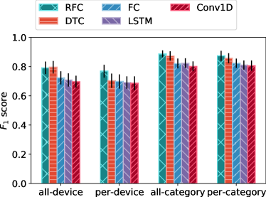
Figure 2. Average $F_{1}$ score of various models using a training window of various sizes (1-7) over the prediction of up to 7 days ahead.

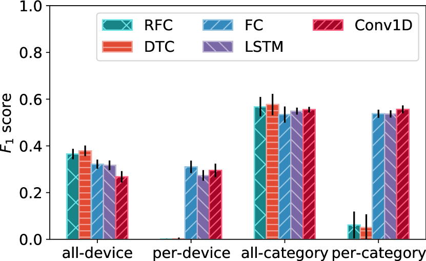
(a) Large Test-bed

(b) Small Test-bed

Figure 3. Average $F_{1}$ score of models trained on 7 day window of idle data and tested on active data of the large and the small test-bed.

The RFC and DTC model perform very similarly in all but the per-device model group. In all cases they slightly outperform the models based on neural networks. The average difference of $F_{1}$ score between the tree-based and the NN models is $0.06$

Generally speaking, all models perform better with the category classification than with the device classification. The average $F_{1}$ score for the category classification is $0.84$ and for the device classification is $0.73$

Multiclass classifiers overall slightly outperform multiple binary classifiers on average by $0.02$. However, the difference is slightly more visible in the case of device classification where the difference in $F_{1}$ score is $0.034$ compared to the category classification where the difference is $0.007$.

RFC and DTC models marginally outperform all models based on neural networks. The performance of neural network based models is essentially the same. Creating a single multi-classification model slightly outperforms an approach based on multiple binary classification models. This applies to both device and category classification.

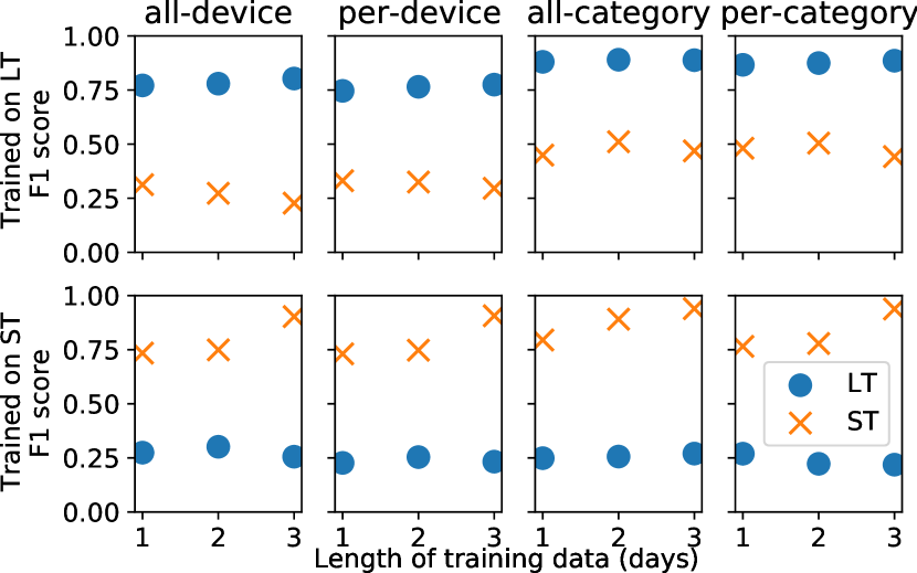
(a) Fully connected model

(b) LSTM model

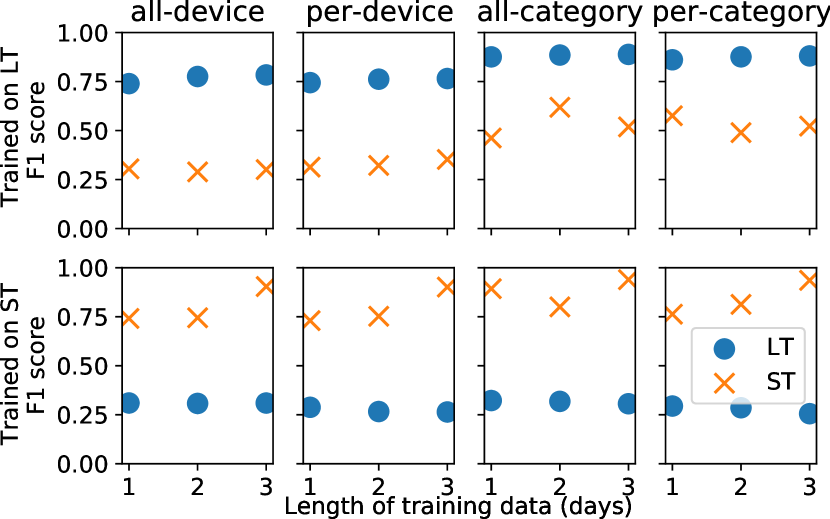
(c) 1D convolutional model

Figure 4. Comparison of $F_{1}$ score of base models (trained on idle data) and updated on the large test-bed (LT, top row) and the small test-bed (ST, bottom row). The mark shows the average $F_{1}$ score for device/category classification achieved over 7 days of active experiments. The x-axis shows how many days (1-3) of data were used to update the model. ◦ denotes score achieved on LT, while × denotes score achieved on ST.

4.3. Active Dataset

Models trained on the idle dataset show a reasonably high $F_{1}$ score suggesting that they can be used for on-line device/category classification of IoT devices in a home environment. Next, we evaluate these models on data collected over seven days of automated experiments on our two test-beds (§3.1): (i) the large test-bed (LT) and (ii) the small test-bed (ST). The active data consist of the mixture of light/medium/heavy usage patterns as described previously (§3.1). For the purpose of evaluation we chose the models which achieved the highest $F_{1}$ score on the idle data from the large test-bed. These models were trained on a seven day window $w=7$. We evaluated these models on active data from both the large and small test-bed. For the purpose of fair evaluation, we included only the devices that were in common in both test-beds.

Figure 3 shows the comparison of all five models on the large (Figure 3(a)) an the small (Figure 3(b)) test-bed. Two facts can be observed: (i) models trained on the idle data of the large test-bed achieve higher $F_{1}$ score on active data collected from the same test-bed rather than the small test-bed, despite containing the same type of devices, (ii) even if the models are trained on the data from the large test-bed, the device/category classification is significantly worse when compared to classification of idle data.

The $F_{1}$ score achieved by all three models based on neural networks was rather similar. The average score achieved on the large test-bed for device (category) classification was $.3$ ($0.54$, respectively). This score is significantly lower than the score achieved on idle data. However, when the same models were tested in the small test-bed, the $F_{1}$ score was halved to only $0.15$ for device classification and decreased to only $0.42$ for the category classification.

RFC and DTC models achieved slightly higher $F_{1}$ score when compared to models based on neural networks, but only in the case of a single model for all devices/categories. However, this score is still significantly lower than the score achieved on the idle dataset. Surprisingly, the per-* model group performed extremely badly when evaluated on the active data. We believe individual models were very fine-tuned for specific type of traffic and therefore achieved very low $F_{1}$ score on a different type of traffic.

This fact supports our argument that it is necessary to keep the models updated locally, with data collected from the household. The results also show that models updated in one household are not applicable in another household, even if the devices are the same.

Because RFC and DTC models do not support updating of the models with new data, we omit them from the further evaluation. As the models trained on the idle dataset performed so poorly on both of active datasets, we updated the models with the data collected during the active experiments. First, we chose the model that achieved on average the highest $F_{1}$ score on all dates of both test-beds. Unsurprisingly, it was a model trained on a 7 day window of data. We refer to this model as the base model. We also tested a model trained on the whole idle dataset. Surprisingly, this model achieved slightly lower average $F_{1}$ score than the best model trained on a 7 day window. This fact suggests overfitting of the model might be a problem and a smaller dataset might achieve higher $F_{1}$ score.

Next, we update the base model with one, two, or three days of data either from the large or the small test-bed. Figure 4 depicts the comparison between these updated models on both test-beds. Two important facts can be observed immediately: (i) updating the base model with active data from the test-bed significantly increases the $F_{1}$ score of device/category classification on the same test-bed and (ii) updating the base model with data from one test-bed increases the $F_{1}$ score of device/category classification of the other test-bed only marginally. These two facts can be observed for both test-beds.

Updating the base model with just one day of active data from the large test-bed increases the average $F_{1}$ score from just $0.3$ to $0.75$ for the device classification and from $0.54$ to $0.87$ for the category classification. Each additional day increases the $F_{1}$ score on average by $0.011$. On the other hand, when the same model is evaluated on the small test-bed, the $F_{1}$ score increases only from $0.15$ to $0.33$ for the device classification and from $0.42$ to $0.5$ for the category classification. Increasing the training dataset by additional days does not yield a better $F_{1}$ score.

Similarly, when the base model is updated with only one day worth of data from the small test-bed, the average $F_{1}$ score raises from just $0.15$ to $0.73$ for the device classification and from just $0.42$ to $0.82$ for the category classification. Adding one more day worth of data increases the $F_{1}$ score by additional $0.02$ in the case of device and $0.015$ in the case of category classification. Using data from all three days, a $F_{1}$ score as high as $0.9$ (up from just $0.15$) for device and $0.94$ (up from just $0.42$) for category classification is achieved. On the other hand, updating the model with the data from the small test-bed has very limited impact on the $F_{1}$ score of the large test-bed classification. The average $F_{1}$ score for the device and the category classification is only $0.27$, and it remains rather stable regardless of the number of days used to update the model.

Models trained on a dataset collected from an idle test-bed are not accurate and fail when are used on active data. Even a small amount of active data can significantly increase the accuracy of the models. However, a model retrained with active data from one test-bed is not applicable on the same type of data in another test-bed. It means that in order to achieve high accuracy, the model needs to be updated with local data.

4.4. Model sizes

The model size is an important factor for being able to run inference on an edge device, because such a device usually has limited main memory. During our first attempts, the RFC and DTC models did not fit into the main memory, hence inference could not be run at the edge device. Therefore, for these two cases, we performed a hyperparameter (e.g., the number of estimators or the depth of the tree) search to tune the model size while maintaining comparable accuracy.

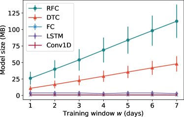
Figure 5. Average model sizes for different types of models for various training windows. The models are from the all-device group.

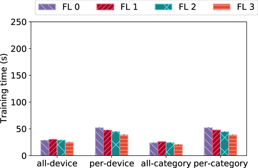
(a) Fully connected model

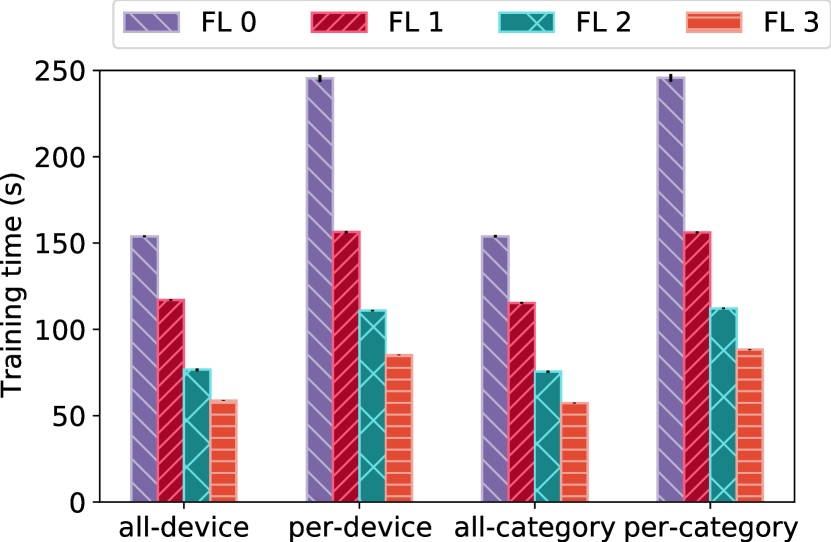
(b) LSTM model

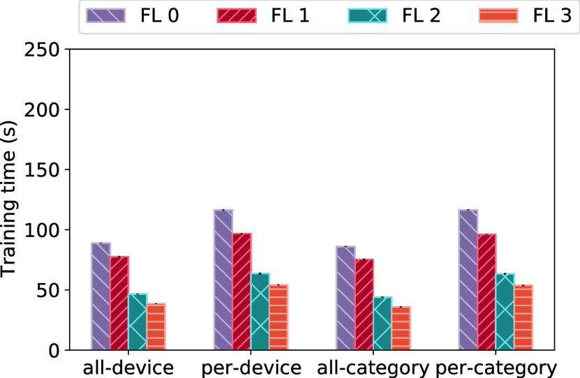
(c) 1D convolutional model

Figure 6. Average training time on RPi4 with different numbers of frozen layers (0, 1, 2 or 3 layers).

Figure 5 shows the sizes of the models in MB for all types of ML models depending on the length of the training window $w$. The figure shows the average size of the all-device group of models. The model sizes of RFC and DTC are increasing linearly with the length of the training window, as the size depends on the size of the training set. On the other hand, the size of the models based on neural networks remains constant. In this case, the type, size, and number of layers influence how many weights there are in the model, and this influences their final size.

The model size of RFC and DTC depends on the number of data points in the training dataset. As we have shown previously, the models need to be updated, and they need to updated locally. Therefore, solutions based on RFC or DTC are not scalable. On the other hand, models based on neural networks can be updated without training from scratch, and also their size remains constant. Therefore they are suitable for being deployed at the edge.

5. Training & Inference at the Edge

Since model accuracy decays over time, the models need to be updated frequently through retraining using new incoming data in order to maintain good accuracy. But retraining models in a centralized manner requires shipping data from home IoT networks to the cloud, which presents challenges in terms of scalability and, more importantly, privacy preservation. Instead, updating the model can take place at the edge of the network, on the home gateway device. This has the advantage of not only reducing the communication bandwidth and latency between the gateway device and the central server, but also preserving the user privacy. On the other hand, edge devices have constraints in terms of CPU and memory. In this section, we examine the impact of these constraints on the retraining of models explored in previous sections, and on running inference on an edge device. To reduce the computation overhead associated with retraining of the model, we reuse parts of the globally trained NN model by freezing layers of the model. Furthermore, we show that our models can run on a representative edge device, demonstrating that IoT devices can be identified at the edge.

As a representative edge device, we used Raspberry Pi model 4 with 4 GB of RAM. The Raspberry Pi is running the Ubuntu 19.04 operating system with Python 3.6, on which a traditional ML stack was installed (numpy, scipy, pandas, scikit-learn, tensorflow, and keras packages).

5.1. Speed of Model Retraining at the Edge

Given the fact that the $F_{1}$ score of the models decreases over time, we investigated the possibility of updating the model locally at the edge using new traffic data from that respective home IoT network. However, we did not start training from scratch, but we used the global model downloaded from a central server. Additionally, we evaluated how freezing different numbers of layers of the neural network (zero, one, two and three layers) influences the training time and $F_{1}$ score of the model. Freezing zero layers means updating the whole model, i.e., re-computing all weights, while freezing three layers means updating only the last layer, i.e., re-computing only a small fraction of weights. We use the idle dataset in our retraining experiments. Figure 6 presents the average running time for training the neural network models on the selected edge device (Raspberry Pi 4). In the case of the per-device models, we plot the training time for training a single model for a single device. We trained models for all of our devices, and the training time for each device is approximately the same. Training models for multiple devices on a Raspberry Pi in our testbed takes $43\times t_{per-device}$, where $t_{per-device}$ is the average training time for a single device. Similarly, we plot the training time for training a single model for a single category. As such, the total training time for our six categories is $6\times t_{per-category}$, where $t_{per-category}$ is the average training time for a single category.

For the FC models, in the case of all-device and all-category models, freezing one or two layers does not reduce the training time, while freezing three layers reduces the training time by $11.8\%$ and by $13.3\%$ respectively. This is probably caused by the structure of the FC model, where the number of neurons increases in each layer, i.e., most weights are in the last three layers. The average training time with three frozen layers is $25$ s for all-device, and $20$ s for all-category. On the other hand, in the case of LSTM and Conv1D models, the training time decreases with each additional frozen layer. For LSTM in the case of all-device models, one frozen layer lowers the training time by $24\%$, two frozen layers by $50.2\%$, and three frozen layers by $61.7\%$. The average training time using three frozen layers is $59$ s. For Conv1D all-device models, one frozen layer reduces the training time by $12.7\%$, two frozen layers by $47.6\%$, and the three frozen layers by $56.6\%$. The training time with three frozen layers is $38$ s. The results for all-category are just slightly smaller compared to all-device for both LSTM and Conv1D.

The training times are approximately the same for the per-device and per-category models for all three model types. For brevity we discuss only the per-device results. In the case of the FC models, freezing one layer reduces the training time by $8.5\%$, two layers by $14.1\%$, and three layers by $25.6\%$. The training time when freezing three layers is $38$ s. In the case of LSTM models, freezing one layer reduces the training time by $36.2\%$, two layers by $54.8\%$, and three layers by $65.2\%$. The average training time when freezing three layers is $85$ s. Lastly, for Conv1D models, freezing one layer reduces the training time by $16.7\%$, two layers by $45.3\%$, and three layers by $53.4\%$. The average training time using three frozen layers is $54$ s.

Model retraining is feasible at the edge for a common household for all types of models. The improvement in training time largely depends on the type and the architecture of the neural network. Layer freezing more than halves the training time for LSTM and Conv1D models, while for FC layer freezing reduces the training time modestly.

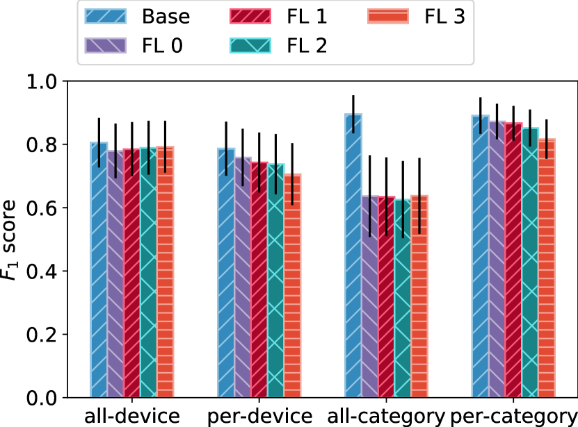
(a) Fully connected model

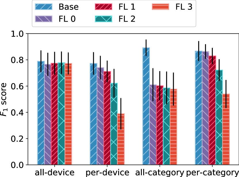
(b) LSTM model

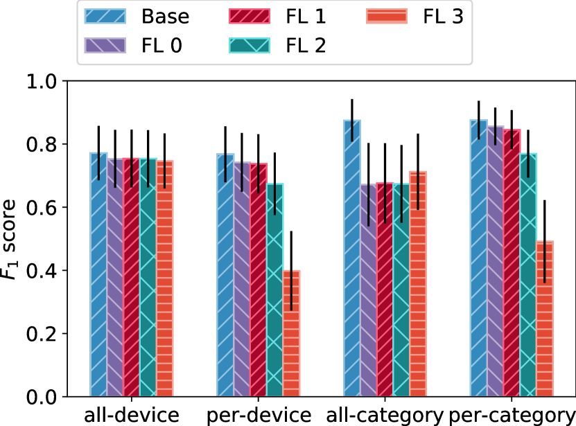
(c) 1D convolutional model

Figure 7. Comparison of $F_{1}$ score with various number of frozen layers.

5.2. $F_{1}$ Score of Retrained Models

To demonstrate how freezing of layers impacts model’s $F_{1}$ score we selected all models already trained on a four day window. The model was updated with the following three days of data while either not freezing any layer or freezing one to three layers. These updated models are effectively trained on seven days worth of data and therefore are compared with models trained on a seven day window. We refer to this model as the base model.

Figure 7 shows how freezing of different numbers of layers influences different types and groups of neural networks. In the case of a all-device classification, the $F_{1}$ score is on average between $0.016$ and $0.02$ lower for all types of neural networks. Surprisingly, the $F_{1}$ score remains virtually the same regardless of the number of frozen layers.

More surprising is the case of the all-category classification. In this case the $F_{1}$ score drops by $0.25$ in the case of FC network, $0.28$ in the case of LSTM, and $0.2$ in the case of Conv1D. Again, the number of frozen layers has a very limited impact on the $F_{1}$ score of the models. The reason for such a dramatic decrease is yet unknown and would require deeper inspection and analysis of the weight updates in the model, which is out of the scope of this paper.

While in the case of all-* group of models there was very little difference in $F_{1}$ score when different numbers of layers were frozen, in the case of per-* group of models, the number of frozen layers has significant influence on the $F_{1}$ score. The least visible impact is with the FC network, where freezing an additional layer decreases the $F_{1}$ score on average by $0.02$ in the case of per-device classification and $0.018$ in the case of per-category classification.

In the case of LSTM models, freezing layers has a much bigger influence on the $F_{1}$ score. Freezing between zero and three layers in the per-device group, decreases the $F_{1}$ score by $0.03,0.06,0.15$ and as much as $0.38$ when compared with the base model. Similarly, in the case of per-category group, freezing between zero and three layers leads to decrease of $0,0.4,0.14,\text{and }0.33$.

Similarly, in the case of Conv1D model, the influence of freezing different numbers of layers has a significant impact on the $F_{1}$ score. Not freezing any layer decreases the $F_{1}$ score by $0.02$ points in per-device and per-category groups when compared to the base scenario. Freezing one layer reduces $F_{1}$ score by $0.03$ (in both scenarios), two layers by $0.09$ and $0.1$ in per-device and per-category group respectively, and three layers by as much as $0.37$ and $0.38$ points.

Freezing layers can noticeably decrease the accuracy of the model. The decrease depends on the type and the structure of the model. In a real world scenario, the number of frozen layers could either be chosen by the entity (e.g., manufacturer) providing the base model, or by the edge device depending on its computational power and the number of models requiring updating.

5.3. Speed of Model Inference at the Edge

We run the model inference on the Raspberry Pi 4 to evaluate average inference running times. We use a lightweight version of the TensorFlow library called TensorFlow Lite (tfl, [n.d.]), specifically designed for edge devices. All models were converted to a format supported by this library. In the case of per-* models, the inference is executed on all models sequentially, and the model with the highest probability is selected as the output device/category. Therefore, the inference time depends on the number of devices/categories that we need to classify. Generally, the time scales linearly with the number of devices/categories.

We run inference using the three neural network models (FC, LSTM, Conv1D), as detailed in (§3). We first randomly select 1000, 10,000, and 100,000 samples (flows) from our dataset. We feed the samples to each model, and we measure how long inference takes for this number of samples. Figure 8 presents the results for average inference time of 100K samples. Results from our experiments show that the total time scales linearly depending on the number of samples. Therefore, we omit figures showing the inference time for 1K and 10K samples. The average inference time are very similar for all model groups. We discuss for brevity the results for the all-device group of models. The average inference time for FC network is $5.3$ s, for LSTM $697$ s, and for Conv1D is $10.8$ s.

The results for per-device and per-category models are presented for only one instance of the model being run. Thus, for inference  per-device or per-category, all the models for all of the devices are run sequentially to determine the device’s type or category. This means that inference takes in our case $43\times t_{per-device}$, where $t_{per-device}$ is the average inference time for a single device. Similarly, the total inference time for our six categories is $6\times t_{per-category}$, where $t_{per-category}$ is the average inference time for a single category.

The results are similar across the four groups of models for each type of neural network model. However, the inference time for LSTM models is considerably larger than in the case of FC network and Conv1D models, with FC being the fastest. LSTM inference time is approximately $140$ times larger than FC. Conv1D inference time is double the time of the FC models.

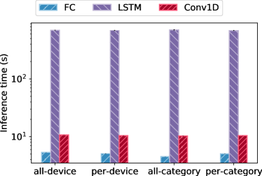
Figure 8. Average inference time on RPi4 of 100K samples using TensorFlow Lite.

6. Discussion & Limitations

Table 4. Classification of an unknown device into a category.

Surveillance		Media		Audio		Hub		Appliance		Home automation
Model	$F_{1}$ score	Model	$F_{1}$ score	Model	$F_{1}$ score	Model	$F_{1}$ score	Model	$F_{1}$ score	Model	$F_{1}$ score
RFC	0.444	RFC	0.176	RFC	0.616	RFC	0.084	RFC	0.119	RFC	0.405
DTC	0.407	DTC	0.168	DTC	0.617	DTC	0.085	DTC	0.120	DTC	0.409
FC	0.399	FC	0.154	FC	0.611	FC	0.090	FC	0.078	FC	0.458
LSTM	0.405	LSTM	0.135	LSTM	0.623	LSTM	0.099	LSTM	0.099	LSTM	0.462
Conv1D	0.338	Conv1D	0.191	Conv1D	0.620	Conv1D	0.134	Conv1D	0.065	Conv1D	0.471

There are a number of future directions that we would like to explore. An important parameter of online IoT device identification is how often do we need to retrain the models on the edge device. Training just one model for all devices/categories can be done in tens of seconds. Therefore, training for this type of models is not prohibitive and can be done often, for example during the night when the IoT gateway is less loaded due to lower network traffic. On the other hand, frequent updating of models for each device and category might not be feasible if the respective home IoT network has a considerable number of devices and categories. In our case, having tens of devices means that training a separate model for each device and category would take approximately four hours in the best case scenario. Retraining a separate model for each category would take approximately five minutes for six categories. As we have shown, the time it takes to retrain the models depends on the type of neural networks, and which part of the network is retrained, i.e., whether part of the model is frozen or not. There is a trade-off between the decay of model accuracy per day and the computation incurred by retraining the model.

In a scenario where a user connects a new device to their home network, we investigate and evaluate whether it is possible to infer the device category. For that purpose we trained all our models of different types and training lengths with data omitting exactly one IoT device. This process was repeated for every device in our test-bed. This led to training of more than 158,000 ML models. These models were evaluated using the data collected from the omitted IoT device.

Table 4 shows the average $F_{1}$ score over all window sizes for each model type. We see that different models perform similarly and there is no major outlier. The lowest score was achieved for the appliance and the hubs category. Surprisingly, the media category achieved a rather low score as well. On the other hand, surveillance and home-automation category achieved on average a rather high $F_{1}$ score of $40\%$ and $44\%$ respectively. The highest score was achieved by the audio category ($62\%$). However, this category contained only five devices, four of which were from the same manufacturer (Amazon Alexa device). Therefore, these devices have very similar network traffic which can lead to high category classification even if a device is omitted from the training set.

Our results show that accurate inference of the category of a newly connected device is hard and is an important direction for further research.

While we have explored the influence of freezing different parts of the model and its implications on the $F_{1}$ score of the model, we evaluated only the average change over all devices. It is possible that freezing of layers influence different devices in different way. Therefore, freezing of different numbers of layers depending on the device should be explored.

While a single model for all devices/categories can be trained faster and achieves higher $F_{1}$ score, given that every household is essentially unique with a different number and types of devices, it is impossible to create a model for every permutation of IoT devices. On the other hand, having a separate model for each device increases the training, as well as inference time. It also achieves lower $F_{1}$ score. Therefore, we plan to investigate the possibility of merging retrained binary classification models into a single multi-classification model at the edge.

Because we focus on online traffic classification, we rely on features that can be readily extracted from the current network flow. Other approaches, where historical data are included, e.g., number of IPs contacted in the last hour or DNS requests made, might be more reliable and lead to higher $F_{1}$ score. Therefore, we plan to investigate whether adding historical data as feature improves the classification accuracy.

We focus on three most common neural networks which are widely popular. We mostly use the same type of layer in the whole model in order to evaluate influence of the specific type of the network on the training and inference time, as well as on the $F_{1}$ score. A combination of several layer types might lead to higher classification accuracy.

We have shown that a single device might behave differently depending on the other devices in the network. This was demonstrated when a model trained on one test-bed achieved very low $F_{1}$ score on the other test-bed and vice versa. Therefore we would like to study dynamics of the networks and how the network profile of devices changes depending on adding or removing other devices from the network.

One possible fallacy of model retraining is the possibility of malicious devices being brought into the network. When retraining takes place, these might effectively “poison” the model, allowing their malicious behavior to go undetected. However, this can be mitigated through adding signatures or obfuscated code on the device (Celik et al., 2019), and it is out of scope for this work.

7. Conclusion

In this paper, we trained and evaluated over 200,000 different ML models for IoT device fingerprinting using full packet samples from a large number of IoT devices and categories, in active and idle mode. We showed that the accuracy of the model decays over time, irrespective of the size of the training set. A trained model used the following day achieves on average $78\%$ accuracy. This accuracy drops to $72\%$ after a week and only $52\%$ after two weeks of usage. We also showed that a model trained on one dataset performs poorly when tested on a different dataset even from the same test-bed. The accuracy of a model trained on idle dataset drops to only $30\%$ when evaluated on active data from the same test-bed and staggering $15\%$ when evaluated on a different test-bed contains a subset of IoT devices. We also show that even though retraining a model on an active dataset from one test-bed increases the accuracy on the said test-bed from $30\%$ to $78\%$, it has very little impact on the other test-bed, increasing accuracy from $15\%$ to only $33\%$. The similar results were obtained when models were retrained on the second test-bed and evaluated on the first one. Our results clearly demonstrate that models need to be regularly retrained locally at the edge.

To address these issues, we evaluated model retraining at the edge using a representative edge device (Raspberry Pi 4). We showed that it is feasible to update a globally trained model with local data and achieve comparable accuracy to the globally trained model. We also showed that it is possible to speed up the training by partially freezing the parts of a model, and evaluated the impact of freezing on the training time (can be cut by more than $66\%$, depending on the model) and the accuracy of the model (drop by less than $2\%$).

Our results clearly indicate that creating one general model is not a feasible solution for efficient IoT device identification at the edge due to the accuracy decay over time. The solution for this problem is to keep the model updated with local data and perform regular model retraining at the edge. In this way, the home gateway is capable of performing online IoT device classification, while retraining the models regularly during idle periods. Our findings can be a step towards accurate and real-time IoT anomaly detection and threat mitigation.

References

- (1)
- joy ([n.d.]) [n.d.]. A package for capturing and analyzing network flow data and intraflow data, for network research, forensics, and security monitoring. https://github.com/cisco/joy. [Online; accessed May 2020].
- tfl ([n.d.]) [n.d.]. TensorFlow Lite. https://www.tensorflow.org/lite. [Online; accessed Jan 2020].
- Aceto et al. (2019) G. Aceto, D. Ciuonzo, A. Montieri, and A. Pescapé. 2019. Mobile Encrypted Traffic Classification Using Deep Learning: Experimental Evaluation, Lessons Learned, and Challenges. IEEE Transactions on Network and Service Management 16, 2 (2019), 445–458.
- Alrawi et al. (2019) O. Alrawi, C. Lever, M. Antonakakis, and F. Monrose. 2019. SoK: Security Evaluation of Home-Based IoT Deployments. In 2019 IEEE Symposium on Security and Privacy (SP). IEEE Computer Society, Los Alamitos, CA, USA. https://doi.org/10.1109/SP.2019.00013
- Amar et al. (2018) Yousef Amar, Hamed Haddadi, Richard Mortier, Anthony Brown, James A. Colley, and Andy Crabtree. 2018. An Analysis of Home IoT Network Traffic and Behaviour. CoRR abs/1803.05368 (2018). arXiv:1803.05368 http://arxiv.org/abs/1803.05368
- Apthorpe et al. (2016) Noah Apthorpe, Dillon Reisman, and Nick Feamster. 2016. A Smart Home is No Castle: Privacy Vulnerabilities of Encrypted IoT Traffic. Workshop on Data and Algorithmic Transparency (DAT’16) (2016). http://arxiv.org/abs/1705.06805
- Banbury et al. (2020) Colby R. Banbury, Vijay Janapa Reddi, Max Lam, William Fu, Amin Fazel, Jeremy Holleman, Xinyuan Huang, Robert Hurtado, David Kanter, Anton Lokhmotov, David Patterson, Danilo Pau, Jae sun Seo, Jeff Sieracki, Urmish Thakker, Marian Verhelst, and Poonam Yadav. 2020. Benchmarking TinyML Systems: Challenges and Direction. In Proceedings of the 3rd MLSys Conference (Austin, TX, USA) (MLSys’20). arXiv:2003.04821
- Breiman (2001) Leo Breiman. 2001. Random Forests. Machine Learning 45, 1 (2001), 5–32. https://doi.org/10.1023/A:1010933404324
- Celik et al. (2019) Z. Berkay Celik, Gang Tan, and Patrick McDaniel. 2019. IoTGuard: Dynamic Enforcement of Security and Safety Policy in Commodity IoT. In Network and Distributed System Security Symposium (NDSS). San Diego, CA. https://www.ndss-symposium.org/wp-content/uploads/2019/02/ndss2019_07A-1_Celik_paper.pdf
- Feng et al. (2018) Xuan Feng, Qiang Li, Haining Wang, and Limin Sun. 2018. Acquisitional Rule-Based Engine for Discovering Internet-of-Thing Devices. In Proceedings of the 27th USENIX Conference on Security Symposium (Baltimore, MD, USA) (SEC’18). USENIX Association, USA, 327 – 341.
- Feraudo et al. (2020) Angelo Feraudo, Poonam Yadav, Vadim Safronov, Diana Andreea Popescu, Richard Mortier, Shiqiang Wang, Paolo Bellavista, and Jon Crowcroft. 2020. CoLearn: Enabling Federated Learning in MUD compliant IoT Edge Networks. In In 3rd International Workshop on Edge Systems, Analytics and Networking (EdgeSys’20). ACM, New York.
- Goodfellow et al. (2016) Ian Goodfellow, Yoshua Bengio, and Aaron Courville. 2016. Deep Learning. MIT Press. http://www.deeplearningbook.org.
- Hackeling (2014) Gavin Hackeling. 2014. Mastering Machine Learning With Scikit-Learn. Packt Publishing.
- Hafeez et al. (2020) I. Hafeez, M. Antikainen, A. Y. Ding, and S. Tarkoma. 2020. IoT-KEEPER: Detecting Malicious IoT Network Activity Using Online Traffic Analysis at the Edge. IEEE Transactions on Network and Service Management 17, 1 (2020), 45–59.
- Hochreiter and Schmidhuber (1997) Sepp Hochreiter and Jürgen Schmidhuber. 1997. Long Short-Term Memory. Neural Comput. 9, 8 (Nov. 1997), 1735–1780. https://doi.org/10.1162/neco.1997.9.8.1735
- Kusupati et al. (2018) Aditya Kusupati, Manish Singh, Kush Bhatia, Ashish Kumar, Prateek Jain, and Manik Varma. 2018. FastGRNN: A Fast, Accurate, Stable and Tiny Kilobyte Sized Gated Recurrent Neural Network. In Proceedings of the 32nd International Conference on Neural Information Processing Systems (Montréal, Canada) (NIPS’18). Curran Associates Inc., Red Hook, NY, USA, 9031–9042.
- Lakshminarayanan et al. (2014) Balaji Lakshminarayanan, Daniel M Roy, and Yee Whye Teh. 2014. Mondrian Forests: Efficient Online Random Forests. In Advances in Neural Information Processing Systems 27, Z. Ghahramani, M. Welling, C. Cortes, N. D. Lawrence, and K. Q. Weinberger (Eds.). Curran Associates, Inc., 3140–3148. http://papers.nips.cc/paper/5234-mondrian-forests-efficient-online-random-forests.pdf
- Lear et al. (2019) E. Lear, R. Droms, and D. Romascanu. 2019. Manufacturer Usage Description Specification. RFC 8520.
- LeCun and Bengio (1995) Yann LeCun and Yoshua Bengio. 1995. Convolutional Networks for Images, Speech, and Time Series. In The Handbook of Brain Theory and Neural Networks. MIT Press, Cambridge, MA, USA, 255–258.
- Lopez-Martin et al. (2017) M. Lopez-Martin, B. Carro, A. Sanchez-Esguevillas, and J. Lloret. 2017. Network Traffic Classifier With Convolutional and Recurrent Neural Networks for Internet of Things. IEEE Access 5 (2017), 18042–18050.
- Magid et al. (2019) S. Abdel Magid, F. Petrini, and B. Dezfouli. 2019. Image classification on IoT edge devices: profiling and modeling. Cluster Computing (2019). https://doi.org/10.1007/s10586-019-02971-9
- Meidan et al. (2017) Yair Meidan, Michael Bohadana, Asaf Shabtai, Juan David Guarnizo, Martín Ochoa, Nils Ole Tippenhauer, and Yuval Elovici. 2017. ProfilIoT: A Machine Learning Approach for IoT Device Identification Based on Network Traffic Analysis. In Proceedings of the Symposium on Applied Computing (Marrakech, Morocco) (SAC ’17). Association for Computing Machinery, New York, NY, USA, 506–509. https://doi.org/10.1145/3019612.3019878
- Miettinen et al. (2017) M. Miettinen, S. Marchal, I. Hafeez, N. Asokan, A. Sadeghi, and S. Tarkoma. 2017. IoT SENTINEL: Automated Device-Type Identification for Security Enforcement in IoT. In 2017 IEEE 37th International Conference on Distributed Computing Systems (ICDCS). 2177–2184.
- Moore and Zuev (2005) Andrew W. Moore and Denis Zuev. 2005. Internet Traffic Classification Using Bayesian Analysis Techniques. In Proceedings of the 2005 ACM SIGMETRICS International Conference on Measurement and Modeling of Computer Systems. Association for Computing Machinery, New York, NY, USA. https://doi.org/10.1145/1064212.1064220
- Nguyen et al. (2019) T. D. Nguyen, S. Marchal, M. Miettinen, H. Fereidooni, N. Asokan, and A. Sadeghi. 2019. DÏoT: A Federated Self-learning Anomaly Detection System for IoT. In 2019 IEEE 39th International Conference on Distributed Computing Systems (ICDCS). 756–767.
- Nguyen and Armitage (2008) T. T. T. Nguyen and G. Armitage. 2008. A survey of techniques for internet traffic classification using machine learning. IEEE Communications Surveys Tutorials 10, 4 (2008), 56–76.
- Ortiz et al. (2019) Jorge Ortiz, Catherine Crawford, and Franck Le. 2019. DeviceMien: Network Device Behavior Modeling for Identifying Unknown IoT Devices. In Proceedings of the International Conference on Internet of Things Design and Implementation (Montreal, Quebec, Canada) (IoTDI ’19). Association for Computing Machinery, New York, NY, USA, 106–117. https://doi.org/10.1145/3302505.3310073
- Pacheco et al. (2019) F. Pacheco, E. Exposito, M. Gineste, C. Baudoin, and J. Aguilar. 2019. Towards the Deployment of Machine Learning Solutions in Network Traffic Classification: A Systematic Survey. IEEE Communications Surveys Tutorials 21, 2 (2019), 1988–2014.
- Painsky and Rosset (2019) A. Painsky and S. Rosset. 2019. Lossless Compression of Random Forests. Journal of Computer Science and Technology 34 (2019), 494–506. https://doi.org/10.1007/s11390-019-1921-0
- Pashamokhtari et al. (2020) A. Pashamokhtari, H. H. Gharakheili, and V. Sivaraman. 2020. Progressive Monitoring of IoT Networks Using SDN and Cost-Effective Traffic Signatures. In 2020 Workshop on Emerging Technologies for Security in IoT (ETSecIoT). 1–6.
- Pinheiro et al. (2019) Antonio Pinheiro, Jeandro Bezerra, Caio Burgardt, and Divanilson Campelo. 2019. Identifying IoT devices and events based on packet length from encrypted traffic. Computer Communications 144 (05 2019), 8–17. https://doi.org/10.1016/j.comcom.2019.05.012
- Ren et al. (2019) Jingjing Ren, Daniel J. Dubois, David Choffnes, Anna Maria Mandalari, Roman Kolcun, and Hamed Haddadi. 2019. Information Exposure for Consumer IoT Devices: A Multidimensional, Network-Informed Measurement Approach. In Proc. of the Internet Measurement Conference (IMC).
- Safavian and Landgrebe (1991) S. R. Safavian and D. Landgrebe. 1991. A survey of decision tree classifier methodology. IEEE Transactions on Systems, Man, and Cybernetics 21, 3 (1991), 660–674.
- Saffari et al. (2009) A. Saffari, C. Leistner, J. Santner, M. Godec, and H. Bischof. 2009. On-line Random Forests. In 2009 IEEE 12th International Conference on Computer Vision Workshops, ICCV Workshops. 1393–1400.
- Sivanathan et al. (2019) A. Sivanathan, H. H. Gharakheili, F. Loi, A. Radford, C. Wijenayake, A. Vishwanath, and V. Sivaraman. 2019. Classifying IoT Devices in Smart Environments Using Network Traffic Characteristics. IEEE Transactions on Mobile Computing 18, 8 (2019), 1745–1759.
- Sun et al. (2014) Chong Sun, Narasimhan Rampalli, Frank Yang, and AnHai Doan. 2014. Chimera: Large-scale Classification Using Machine Learning, Rules, and Crowdsourcing. Proc. VLDB Endow. 7, 13 (Aug. 2014), 1529–1540. https://doi.org/10.14778/2733004.2733024
- Tahaei et al. (2020) Hamid Tahaei, Firdaus Afifi, Adeleh Asemi, Faiz Zaki, and Nor Badrul Anuar. 2020. The rise of traffic classification in IoT networks: A survey. Journal of Network and Computer Applications 154 (2020), 102538. https://doi.org/10.1016/j.jnca.2020.102538
- Trimananda et al. (2020) Rahmadi Trimananda, Janus Varmarken, Athina Markopoulou, and Brian Demsky. 2020. Packet-Level Signatures for Smart Home Device Events. In Network and Distributed Systems Security (NDSS) Symposium 2020. https://doi.org/10.14722/ndss.2020.24097
- Wang et al. (2017) W. Wang, M. Zhu, J. Wang, X. Zeng, and Z. Yang. 2017. End-to-end encrypted traffic classification with one-dimensional convolution neural networks. In 2017 IEEE International Conference on Intelligence and Security Informatics (ISI). 43–48.
- Wang et al. (2020) Xin Wang, Shuhui Chen, and Jinshu Su. 2020. Real Network Traffic Collection and Deep Learning for Mobile App Identification. Wireless Communications and Mobile Computing 2020 (19 Feb 2020), 4707909. https://doi.org/10.1155/2020/4707909
- Yadav et al. (2019) Poonam Yadav, Qi Li, Richard Mortier, and Anthony Brown. 2019. Network Service Dependencies in Commodity Internet-of-things Devices. In Proceedings of the International Conference on Internet of Things Design and Implementation (Montreal, Quebec, Canada) (IoTDI ’19). ACM, New York, NY, USA, 202–212. https://doi.org/10.1145/3302505.3310082
- Yang et al. (2019) C. Yang, W. Jiang, and Z. Guo. 2019. Time Series Data Classification Based on Dual Path CNN-RNN Cascade Network. IEEE Access 7 (2019), 155304–155312.