Solving Symmetric and Positive Definite Second-Order Cone Linear Complementarity Problem by A Rational Krylov Subspace Method

Abstract

The second-order cone linear complementarity problem (SOCLCP) is a generalization of the classical linear complementarity problem. It has been known that SOCLCP, with the globally uniquely solvable property, is essentially equivalent to a zero-finding problem in which the associated function bears much similarity to the transfer function in model reduction [SIAM J. Sci. Comput., 37 (2015), pp. A2046–A2075]. In this paper, we propose a new rational Krylov subspace method to solve the zero-finding problem for the symmetric and positive definite SOCLCP. The algorithm consists of two stages: first, it relies on an extended Krylov subspace to obtain rough approximations of the zero root, and then applies multiple-pole rational Krylov subspace projections iteratively to acquire an accurate solution. Numerical evaluations on various types of SOCLCP examples demonstrate its efficiency and robustness.

Key words. SOCLCP, second-order cone, globally uniquely solvable property, transfer function, rational Krylov subspace method

AMS subject classifications. 90C33, 65K05, 65F99, 65F15, 65F30, 65P99

1 Introduction

For a given symmetric and positive definite $M\in\mathbb{R}^{n\times n}$ and a vector $\boldsymbol{q}\in\mathbb{R}^{n}$, in this paper, we are concerned with the following second-order cone linear complementarity problem:

$$\operatorname{SOCLCP}({\mathbb{K}}^{n},M,\boldsymbol{q}):\quad{\rm find}~{}~{}\boldsymbol{x}\in{\mathbb{K}}^{n}\mbox{ such that}\quad\boldsymbol{q}+M\boldsymbol{x}\in{\mathbb{K}}^{n}\quad\mbox{and}\quad\boldsymbol{x}^{\operatorname{T}}(\boldsymbol{q}+M\boldsymbol{x})=0,$$ (1.1)

where ${\mathbb{K}}^{n}:=\Big{\{}[x_{1},\boldsymbol{x}_{2}^{\operatorname{T}}]^{\operatorname{T}}\in\mathbb{R}\times\mathbb{R}^{n-1}\,:\,\|\boldsymbol{x}_{2}\|_{2}\leq x_{1}\Big{\}}$ is the so-called second-order cone or the the Lorentz cone. The set of solutions of $\operatorname{SOCLCP}({\mathbb{K}}^{n},M,\boldsymbol{q})$ is denoted by $\operatorname{SOL}(M,{\mathbb{K}}^{n},\boldsymbol{q})$.

The $\operatorname{SOCLCP}({\mathbb{K}}^{n},M,\boldsymbol{q})$ is a generalization of the classical linear complementarity problem $\operatorname{SOCLCP}(\mathbb{R}_{+}^{n},M,\boldsymbol{q})$ [7] from the nonnegative cone $\mathbb{R}_{+}^{n}=\{\boldsymbol{x}\in\mathbb{R}^{n}|\boldsymbol{x}\geq 0\}$ to ${\mathbb{K}}^{n}.$ Solvability and many crucial properties of the set of solutions of $\operatorname{SOCLCP}({\mathbb{K}}^{n},M,\boldsymbol{q})$ have been established (see e.g., [4, 5, 6, 10, 15, 16, 31, 32, 35]), which provide foundations for many numerical methods. For example, the notion of globally uniquely solvable (GUS) property for $M$ which states that the linear complementarity problem has a unique solution for any given $\boldsymbol{q}\in\mathbb{R}^{n}$, plays an important role in both $\operatorname{SOCLCP}(\mathbb{R}_{+}^{n},M,\boldsymbol{q})$ [7] and $\operatorname{SOCLCP}({\mathbb{K}}^{n},M,\boldsymbol{q})$ [31]. In particular, for $\operatorname{SOCLCP}({\mathbb{K}}^{n},M,\boldsymbol{q})$, Yang and Yuan [31] proposed an important algebraic characterization of the GUS property. This provides new perspective on $\operatorname{SOCLCP}({\mathbb{K}}^{n},M,\boldsymbol{q})$ and also leads to several efficient numerical methods (see e.g., [31, 33, 34, 35]). A recent work [30] is an factorization-based numerical algorithm that is efficient for small- to medium-size problems. Specifically, the method is based on the full eigen-decomposition of matrix pencil $M-\lambda J$, where

$$J=\operatorname{diag}(1,-1,\ldots,-1),$$ (1.2)

and can be regarded as a direct method, as opposed to iterative methods previously, because computing the full eigen-decomposition, although iterative in nature, is mature enough to be widely considered as direct in applications [8, 12]. Nonetheless, for large scale and sparse problems, such an eigen-decomposition-based method is still very expensive or inapplicable.

The focus of this paper is on the efficient methods for large-scale $\operatorname{SOCLCP}({\mathbb{K}}^{n},M,\boldsymbol{q})$ with $M$ symmetric and positive definite. Our approach follows the same numerical framework of the Krylov subspace method in [35], which generally contains the following three steps:

• transform $\operatorname{SOCLCP}({\mathbb{K}}^{n},M,\boldsymbol{q})$ to a zero-finding problem [35],

• project the zero-finding problem to a much smaller scale problem by certain rational Krylov subspaces,

• solve the projected problem by an efficient zero-finding solver, e.g., the direct method of [30].

Our main contribution is on the second step in which we provide a more effective rational Krylov subspace to improve the performance of the algorithmic framework of [35]. Even though the method of [35] is applicable for more general $\operatorname{SOCLCP}({\mathbb{K}}^{n},M,\boldsymbol{q})$ where $M$ is not necessarily symmetric and positive definite, we will demonstrate that our new Krylov subspace method performs generally better than that of [35] whenever $M$ is symmetric and positive definite.

This paper is organized as follows. In Section 2, we summarize some preliminary theoretical results of $\operatorname{SOCLCP}({\mathbb{K}}^{n},M,\boldsymbol{q})$, most of which are from [35]. In Section 3, we propose our rational Krylov subspace projection method. The numerical approach for the reduced problem in step 3 is discussed in Subsection 3.2. Our numerical evaluation of the new method is carried out in Section 4, where we report our numerical experiments by comparing it with other algorithms. We draw our final remarks in Section 5.

Notation: Throughout this paper, all vectors are column vectors and are typeset in bold lower case letters. The identity matrix in $\mathbb{R}^{n\times n}$ will be denoted by $I_{n}\equiv[\boldsymbol{e}_{1},\boldsymbol{e}_{2},\dots,\boldsymbol{e}_{n}]$, where $\boldsymbol{e}_{i}$ is its $i$ column. For $A\in\mathbb{R}^{n\times m}$, $A^{\operatorname{T}}$ denotes its transpose. The labels ${\cal R}(A)$ and ${\cal N}(A)$ denote the range and kernel of $A$, respectively. Thus, ${\cal R}(A)^{\perp}={\cal N}(A^{\operatorname{T}}),$ where ${\cal R}(A)^{\perp}$ denotes the orthogonal complement of ${\cal R}(A)$. If $A$ is square, then we use $\operatorname{eig}(A)=\{\lambda_{i}(A)\}_{i=1}^{n}$ to represent the set of eigenvalues, and use $A\succ 0$ to indicate $A$ is symmetric and positive definite. Also, both ${\rm orth}(A)$ and ${\rm orth}({\cal R}(A))$ represent the orthonormal basis matrix of ${\cal R}(A)$. For convenience, we shall adopt MATLAB-like format: $\boldsymbol{x}_{(i)}$ is the $i$th element of $\boldsymbol{x}$ and $A_{(i,j)}$ is the $(i,j)$th entry of $A$, where $(i:j)$ stands for the set of integers from $i$ to $j$ inclusive, and $A_{(k:\ell,i:j)}$ is the submatrix of $A$ that consists of intersections from row $k$ to row $\ell$ and column $i$ to column $j$. The $\ell$th Krylov subspace generated by $A\in\mathbb{R}^{n\times n}$ on $\boldsymbol{x}\in\mathbb{R}^{n}$ is defined as

$${\cal K}_{\ell}(A,\boldsymbol{x})={\rm span}(\boldsymbol{x},A\boldsymbol{x},\dots,A^{\ell-1}\boldsymbol{x}).$$

When $A$ is also invertible, the $(\ell,k)$th extended Krylov subspace [18, 24] of $A$ on $\boldsymbol{x}$ is defined as

$${\cal K}_{\ell,k}^{\operatorname{ext}}(A,\boldsymbol{x})={\rm span}(\boldsymbol{x},A\boldsymbol{x},\dots,A^{\ell-1}\boldsymbol{x};A^{-1}\boldsymbol{x},A\boldsymbol{x},A^{-2}\boldsymbol{x},\dots,A^{k-1}\boldsymbol{x},A^{k}\boldsymbol{x}).$$

2 Preliminaries

In this section, we first briefly review preliminary results on $\operatorname{SOCLCP}({\mathbb{K}}^{n},M,\boldsymbol{q})$ (1.1). We begin with a characterization of the solution which describes three mutually exclusive cases for the solution of $\operatorname{SOCLCP}({\mathbb{K}}^{n},M,\boldsymbol{q})$.

Theorem 2.1 ([34]).

There are three mutually exclusive cases for the solution $\boldsymbol{x}\in\operatorname{SOL}({\mathbb{K}}^{n},M,\boldsymbol{q})$, namely:

• $\boldsymbol{q}\in{\mathbb{K}}^{n}$ (which implies that $\boldsymbol{x}=\mathbf{0}$ is the solution);

• $\operatorname{SOL}({\mathbb{K}}^{n},M,\boldsymbol{q})\supseteq\{\boldsymbol{x}\in{\mathbb{K}}^{n}\,:\,M\boldsymbol{x}+\boldsymbol{q}=\mathbf{0}\}\neq\varnothing$;

• there exists $s_{*}>0$ such that $M\boldsymbol{x}+\boldsymbol{q}=s_{*}J_{n}\boldsymbol{x}\in\partial({\mathbb{K}}^{n})$, where $\partial({\mathbb{K}}^{n})=\Big{\{}[x_{1},\boldsymbol{x}_{2}^{\operatorname{T}}]^{\operatorname{T}}\in\mathbb{R}\times\mathbb{R}^{n-1}\,:\,\|\boldsymbol{x}_{2}\|_{2}=x_{1}\Big{\}}$ denotes the boundary of ${\mathbb{K}}^{n}$, and $J_{n}$ is given in (1.2).

Note that the first case (C1) is trivially checkable. The second case (C2) can be handled by solving $M\boldsymbol{x}=-\boldsymbol{q}$. It is the third case (C3) that needs sophisticated treatments and leads to different numerical methods. For example, for (C3), [30, 35] consider transforming $\operatorname{SOCLCP}({\mathbb{K}}^{n},M,\boldsymbol{q})$ into a zero-finding problem. To see this, note that

$$\operatorname{eig}(MJ_{n})=\operatorname{eig}(J_{n}M)=\operatorname{eig}(M,J_{n}),$$

where $\operatorname{eig}(M,J_{n})$ denotes the eigenvalues of the matrix pencil $M-\lambda J_{n}$. In fact, $M-\lambda J_{n}=(MJ_{n}-\lambda I_{n})J_{n}=J_{n}(J_{n}M-\lambda I_{n})$ implies

$$\det(M-\lambda J_{n})=(-1)^{n-1}\det(MJ_{n}-\lambda I_{n})=(-1)^{n-1}\det(J_{n}M-\lambda I_{n}).$$

Theorem 2.2 ([35]).

Suppose $s\in\mathbb{R}$ is not an eigenvalue of $MJ_{n}$. Let

$$\boldsymbol{x}(s)\equiv\begin{bmatrix}x_{1}(s)\\ \boldsymbol{x}_{2}(s)\\ \end{bmatrix}:=-(M-sJ_{n})^{-1}\boldsymbol{q},$$

where $J_{n}$ is given by (1.2). Then $\boldsymbol{x}(s)\in\partial({\mathbb{K}}^{n})$ if and only if $x_{1}(s)>0$ and $h(s)=0$, where

$$h(s):=\boldsymbol{x}(s)^{\operatorname{T}}J_{n}\boldsymbol{x}(s)=\boldsymbol{q}^{\operatorname{T}}(M-sJ_{n})^{-\operatorname{T}}J_{n}(M-sJ_{n})^{-1}\boldsymbol{q}.$$ (2.1)

Returning the third case (C3) in Theorem 2.1, we have $(M-s_{*}J_{n})\boldsymbol{x}=-\boldsymbol{q}$ and $\boldsymbol{x}\in\partial({\mathbb{K}}^{n})$. Thus if $s_{*}$ is not an eigenvalue of $MJ_{n}$, then $h(s_{*})=0$, a zero-finding problem. The problem can be further simplified whenever $M$ admits the GUS property [31, 33, 34]. A complete algebraic-geometric characterization of $\operatorname{SOCLCP}({\mathbb{K}}^{n},M,\boldsymbol{q})$ (1.1) with such a property has been established in [31, 33, 34]. As one of the key results, it is proved that $MJ_{n}$ has exactly one positive eigenvalue $\tau$ in $[0,+\infty)$. The reader is referred to [35, Theorem 2.4] for more properties. As a summary, we provide basic facts of the location of the zero root $s_{*}$ in Corollary 2.1, Table 2.1 and Figure 2.1, and suggest [35] for a more detailed discussion.

Table 2.1: The sign of $h(s)$ on $(0,\infty)$ in terms of location of $\boldsymbol{q}$ [35].

cases	where is $\boldsymbol{q}$?	solution $x_{*}$ or $h(s)$
1	$\boldsymbol{q}\in{\mathbb{K}}^{n}$	$0=\boldsymbol{x}_{*}\in\operatorname{SOL}({\mathbb{K}}^{n},M,\boldsymbol{q})$
2	$\boldsymbol{q}\in-M{\mathbb{K}}^{n}$	$-M^{-1}\boldsymbol{q}=\boldsymbol{x}_{*}\in\operatorname{SOL}({\mathbb{K}}^{n},M,\boldsymbol{q})$
3	$\begin{array}[]{c}\boldsymbol{q}\in(-{\mathbb{K}}^{n})\backslash(-M{\mathbb{K}}^{n}),\\ \boldsymbol{q}\not\in{\cal R}(M-\tau J)\end{array}$	$h(s)=\left\{\begin{array}[]{cl}-&\mbox{for}\,\,s\in(0,s_{*}),\\ 0&\mbox{for}\,\,s=s_{*},\\ +&\mbox{for}\,\,s\in(s_{*},\tau),\\ +&\mbox{for}\,\,s\in(\tau,\infty).\end{array}\right.$
4	$\begin{array}[]{c}\boldsymbol{q}\in M{\mathbb{K}}^{n}\backslash{\mathbb{K}}^{n},\\ \boldsymbol{q}\not\in{\cal R}(M-\tau J)\end{array}$	$h(s)=\left\{\begin{array}[]{cl}+&\mbox{for}\,\,s\in(0,\tau),\\ +&\mbox{for}\,\,s\in(\tau,s_{*}),\\ 0&\mbox{for}\,\,s=s_{*},\\ -&\mbox{for}\,\,s\in(s_{*},\infty).\end{array}\right.$
5	$\begin{array}[]{c}\boldsymbol{q}\not\in(-M{\mathbb{K}}^{n})\cup M{\mathbb{K}}^{n}\cup{\mathbb{K}}^{n}\cup(-{\mathbb{K}}^{n}),\\ \boldsymbol{q}\not\in{\cal R}(M-\tau J)\end{array}$	$h(s)=\left\{\begin{array}[]{cl}-&\mbox{for}\,\,s\in(0,s_{*;1}),\\ 0&\mbox{for}\,\,s=s_{*;1},\\ +&\mbox{for}\,\,s\in(s_{*;1},\tau),\\ +&\mbox{for}\,\,s\in(\tau,s_{*;2}),\\ 0&\mbox{for}\,\,s=s_{*;2},\\ -&\mbox{for}\,\,s\in(s_{*;2},\infty).\end{array}\right.$

Figure 2.1: $h(s)$ corresponding to cases 3, 4, and 5 in Table 2.1 [35].

Corollary 2.1.

When $M$ has the GUS property, then the following statements hold:

1. $h(s)$ has a zero in $(0,\tau)$ if and only if $h(0)=\boldsymbol{q}^{\operatorname{T}}M^{-\operatorname{T}}J_{n}M^{-1}\boldsymbol{q}<0$;

2. $h(s)$ has a zero in $(\tau,\infty)$ if and only if $\boldsymbol{q}^{\operatorname{T}}J_{n}\boldsymbol{q}<0$.

The set of all symmetric and positive definite matrices is a subset of GUS [31]. For this special case, we further have more nice properties that can be used for finding the zero root $s_{*}$. In particular, for example, according to [30, Lemma 2.2] (see also Lemma 3.2 later), we know that there is a nonsingular matrix $V\in\mathbb{R}^{n\times n}$ such that

$$V^{\operatorname{T}}MV=\Omega\equiv\operatorname{diag}(\omega_{1},\omega_{2},\ldots,\omega_{n}),\quad V^{\operatorname{T}}J_{n}V=J_{n},$$

where $0<\omega_{1}=\tau$ and $0<\omega_{2}\leq\cdots\leq\omega_{n}$. In particular, $\operatorname{eig}(M,J_{n})=\{\omega_{1},-\omega_{i}\,\,\mbox{for $2\leq i\leq n$}\}$.

3 Rational Krylov Subspace Methods

The transformation from $\operatorname{SOCLCP}({\mathbb{K}}^{n},M,\boldsymbol{q})$ to a zero-finding problem $h(s_{*})=0$ finishes step 1 within the numerical framework of [35]. We next discuss techniques for step 2 to form proper Krylov subspaces onto which the large-scale $\operatorname{SOCLCP}({\mathbb{K}}^{n},M,\boldsymbol{q})$ can be projected and approximately solved.

3.1 Projection via Rational Krylov Subspaces

The motivation of using the rational Krylov subspace is the similarity of the function $h(s)$ (2.1) to transfer functions for certain time-invariant single-input-single-output (SISO) dynamical systems [2, 27]. Both are rational functions that involve the inversions of usually parameter dependent matrices, and it is $(M-sJ_{n})^{-1}$ in our case. In SISO dynamical systems, the transfer function usually has to be evaluated at a wide range of the parameter value, which requires very high computational costs. Model reduction techniques based on Krylov subspace projections [2, 27] are popular and efficient in mitigating high costs of such evaluations. The basic idea is to generate a suitable Krylov subspace and then project the transfer function onto the subspace to yield a reduced transfer function, effectively reduces the original dimension to a few tens or hundreds. The accuracy of approximation by the reduced transfer function is measured by the number of leading terms in its Taylor expansion at a point of interest that match those of the original transfer function in its Taylor expansion at the same point. In model order reduction area, rational Krylov subspace methods are demonstrated efficient in computing system’s $\cal{L}_{\infty}$ norm [1] or pseudospectral abscissa [20], and solving algebraic Riccati equations [25]. For more details, the reader is referred to, e.g., [2, 3, 9, 11, 21, 22, 23, 27] and references therein.

Inspired by the idea in the model reduction, [35] proposes a Krylov subspace method to find the zero $s_{*}$ of $h(s)$. It is an iterative method that can roughly be explained as follows. Suppose $0<s_{0}\in\mathbb{R}$ is a given approximation to $s_{*}$ and let

$$A_{s_{0}}=(M-s_{0}J_{n})^{-1}J_{n},\quad\boldsymbol{b}_{s_{0}}=-(M-s_{0}J_{n})^{-1}\boldsymbol{q}.$$

We have $\boldsymbol{x}(s)=-(M-sJ_{n})^{-1}\boldsymbol{q}=[I_{n}-(s-s_{0})A_{s_{0}}]^{-1}\boldsymbol{b}_{s_{0}}$, and

$$h(s)=\boldsymbol{x}(s)^{\operatorname{T}}J_{n}\boldsymbol{x}(s)=\boldsymbol{b}_{s_{0}}^{\operatorname{T}}[I_{n}-(s-s_{0})A_{s_{0}}]^{-\operatorname{T}}J_{n}[I_{n}-(s-s_{0})A_{s_{0}}]^{-1}\boldsymbol{b}_{s_{0}}.$$

Suppose $s_{0}$ is neither a pole nor a zero of $h(s)$ (in other words, $h(s_{0})\neq 0$ and is finite). This implies $h(s_{0})=\boldsymbol{b}_{s_{0}}^{\operatorname{T}}J_{n}\boldsymbol{b}_{s_{0}}\neq 0$. Let $Y_{\ell}\in\mathbb{R}^{n\times\ell}$ be an orthonormal basis matrix of the Krylov subspace ${\cal K}_{\ell}(A_{s_{0}},\boldsymbol{b}_{s_{0}})$, i.e., $Y_{\ell}^{\operatorname{T}}Y_{\ell}=I_{\ell}$ and ${\cal R}(Y_{\ell})={\cal K}_{\ell}(A_{s_{0}},\boldsymbol{b}_{s_{0}})$. Then the reduced $h(s)$ is given by

$$h_{\ell}(s)=\|\boldsymbol{b}_{s_{0}}\|_{2}^{2}\boldsymbol{e}_{1}^{\operatorname{T}}[I_{\ell}-(s-s_{0})H_{\ell}]^{-\operatorname{T}}Y_{\ell}^{\operatorname{T}}J_{n}Y_{\ell}[I_{\ell}-(s-s_{0})H_{\ell}]^{-1}\boldsymbol{e}_{1},$$

where $H_{\ell}=Y_{\ell}^{\operatorname{T}}A_{s_{0}}Y_{\ell}$. Both $Y_{\ell}$ and $H_{\ell}$ can be efficiently computed by the Arnoldi Process [35, Algorithm 1]. It is proved that [35]

$$h(s)=h_{\ell}(s)+{O}(|s-s_{0}|^{\ell}).$$ (3.1)

Indeed, an immediate implication of (3.1) is that the first $\ell$ leading terms of the Taylor expansions of $h(s)$ and $h_{\ell}(s)$ at $s_{0}$ match, or equivalently, the coefficients of $(s-s_{0})^{i}$ for $i=0,1,\ldots,\ell$, called moments in the expansions, are the same. A particular zero of $h_{\ell}(s)$ is then computed as the next approximation. Since $h_{\ell}(s)$ in general has many zeros, with the help of Table 2.1 and Figure 2.1, the method of [35] picks a particular positive one; conceivably, if $h_{\ell}(s)$ approximates $h(s)$ sufficiently well in the region of interest, a positive zero root exists and solving $h_{\ell}(s)=0$ can be done by equivalently transforming it into an $(\ell-1)\times(\ell-1)$ quadratic eigenvalue problem; the process repeats whenever the updated approximation is not within the given accuracy.

Our improvement of the rational Krylov subspace method over [35] begins with the following approximation theorem when $M\succ 0$.

Theorem 3.1.

If $M$ is symmetric, then

$$h(s)=h_{\ell}(s)+{O}(|s-s_{0}|^{2\ell-1}).$$ (3.2)

Proof.

Let $f(s)=q^{\operatorname{T}}(M-sJ)^{-1}q$ and $f_{\ell}(s)=\|\boldsymbol{b}_{s_{0}}\|_{2}^{2}\boldsymbol{e}_{1}^{\operatorname{T}}[I_{\ell}-(s-s_{0})H_{\ell}]^{-\operatorname{T}}\boldsymbol{e}_{1}$. It can be verified that

$$f^{\prime}(s)=h^{\prime}(s),\quad f_{\ell}^{\prime}(s)=h_{\ell}^{\prime}(s).$$ (3.3)

By [21, Theorem 3.3], we find $f(s)=f_{\ell}(s)+{O}(|s-s_{0}|^{2\ell})$. The equation (3.2) is a consequence of (3.3). ∎

We remark that the approximation accuracy as measured by moment matching given in (3.1) is the best possible when $M$ is in general non-symmetric. For a symmetric $M$, we see from Theorem 3.1 that the number of matched moments doubles.

Instead of [35]’s subspace

$${\cal K}_{\ell}(A_{s_{0}},\boldsymbol{b}_{s_{0}})\equiv{\cal K}_{\ell}((M-s_{0}J_{n})^{-1}J_{n},(M-s_{0}J_{n})^{-1}\boldsymbol{q}),$$

we propose to use a new rational Krylov subspaces to reduce $h(s)$, namely, the sum of several Krylov subspaces in the form of ${\cal K}_{\ell}(A_{s_{i}},\boldsymbol{b}_{s_{i}})$, each of which is expanded at a different point $s_{i}$. Specifically, let $U$ be the orthonormal matrix such that

$${\cal R}(U)=\sum_{i=1}^{j}{\cal K}_{\ell}((M-s_{i}J_{n})^{-1}J_{n},(M-s_{i}J_{n})^{-1}\boldsymbol{q}),$$ (3.4)

and we then reduce $h(s)$ to

$$\hat{h}(s)=\hat{\boldsymbol{q}}^{\operatorname{T}}(\widehat{M}-s\widehat{J})^{-\operatorname{T}}\widehat{J}(\widehat{M}-s\widehat{J})^{-1}\hat{\boldsymbol{q}},$$ (3.5a)

where

$$\widehat{M}=U^{\operatorname{T}}MU,\quad\widehat{J}=U^{\operatorname{T}}J_{n}U,\quad\hat{\boldsymbol{q}}=U^{\operatorname{T}}\boldsymbol{q}.$$ (3.5b)

By using various $s_{i}$ around $s_{*}$, it is hoped that the reduced function $\hat{h}(s)$ is able to qualitatively match better $h(s)$, and therefore, the overall convergence behavior can be improved.

3.2 Solve $\hat{h}(s)=0$

Next, we consider step 3 to solve the zero of the reduced $\hat{h}(s)=0$. We point out that the development in this subsection for $\hat{h}(s)=0$ of form (3.5) works for any $U\in\mathbb{R}^{n\times m}$ with full column rank, i.e., $\operatorname{rank}(U)=m$, not restricted in the basis from a rational Krylov subspace.

To utilize $\hat{h}(s)\approx h(s)$, we need the assumption

$$U^{\operatorname{T}}J_{n}U$$ has one positive eigenvalue and the rest of its eigenvalues are negative. (3.6)

When $U$ has orthonormal columns, this should hold as the number of columns of $U$ increases. In general, $U^{\operatorname{T}}J_{n}U$ has at most one positive eigenvalue.

Lemma 3.1.

Suppose that $U\in\mathbb{R}^{n\times m}$ has orthonormal columns, where $1\leq m<n$. Then $U^{T}J_{n}U$ has at most one positive eigenvalue.

Proof.

Let $U_{\bot}\in\mathbb{R}^{n\times(n-m)}$ such that $[U,U_{\bot}]$ is orthogonal. The eigenvalues of

$$[U,U_{\bot}]^{\operatorname{T}}J_{n}[U,U_{\bot}]=\begin{bmatrix}U^{\operatorname{T}}J_{n}U&U^{\operatorname{T}}J_{n}U_{\bot}\\ U_{\bot}^{\operatorname{T}}J_{n}U&U_{\bot}^{\operatorname{T}}J_{n}U_{\bot}\end{bmatrix}$$

are the same as $J_{n}$. Denote by $\mu_{1}\geq\mu_{2}\geq\cdots\geq\mu_{m}$ the eigenvalues of $U^{\operatorname{T}}J_{n}U$. It suffices to show all $\mu_{i}<0$ for $2\leq i\leq m$. By the Cauchy’s interlacing inequalities [17], we have

$$1\geq\mu_{1}\geq-1,\quad-1\geq\mu_{i}\geq-1\,\,\mbox{for $2\leq i\leq m$}$$

implying $\mu_{i}=-1<0$ for $2\leq i\leq m$, as expected. ∎

Now, we describe two methods for solving $\hat{h}(s)=0$: the first one closely follows the idea in [35] by turning it into a quadratic eigenvalue problem, and it works for both symmetric and nonsymmetric $M$; the second one is the method of [30] and it works for $M\succ 0$ only.

For the first method, we note that the direct transformation to a quadratic eigenvalue problem [35] should be modified to work on (3.5). In particular, suppose $\hat{\boldsymbol{q}}\in\mathbb{R}^{m}$ and $Q\in\mathbb{R}^{m\times m}$ is an orthogonal matrix (for example, the Householder matrix [8]) such that $Q^{T}\hat{\boldsymbol{q}}=\|\hat{\boldsymbol{q}}\|_{2}\boldsymbol{e}_{1}.$ We then can write $\hat{h}(s)$ as follows:

$$\hat{h}(s)=\|\hat{\boldsymbol{q}}\|_{2}^{2}\,\boldsymbol{e}_{1}^{\operatorname{T}}\Big{[}s^{2}Q^{\operatorname{T}}\widehat{J}Q-sQ^{\operatorname{T}}(\widehat{M}^{\operatorname{T}}+\widehat{M})Q+Q^{\operatorname{T}}\widehat{M}\widehat{J}^{-1}\widehat{M}^{\operatorname{T}}Q\Big{]}^{-1}\boldsymbol{e}_{1}.$$

With this preprocess, the method of [35, subsection 6.2] then is applicable.

For the second method related with [30], we need the next lemma which is a straightforward extension of [30, Lemma 2.2] and can be proved in a similar way.

Lemma 3.2.

Suppose $M\succ 0$ and assume (3.6) holds. Then there is a nonsingular matrix $\widehat{V}\in\mathbb{R}^{m\times m}$ such that

$$\widehat{V}^{\operatorname{T}}U^{\operatorname{T}}MU\widehat{V}=\widehat{\Omega}\equiv\operatorname{diag}(\hat{\omega}_{1},\hat{\omega}_{2},\ldots,\hat{\omega}_{m}),\quad\widehat{V}^{\operatorname{T}}U^{\operatorname{T}}J_{n}U\widehat{V}=J_{m},$$ (3.7)

where $0<\hat{\omega}_{1}$ and $0<\hat{\omega}_{2}\leq\cdots\leq\hat{\omega}_{m}$.

Proof.

Write $\widehat{M}=U^{\operatorname{T}}MU$ and $\widehat{J}_{m}=U^{\operatorname{T}}J_{n}U$. Since $\widehat{M}\succ 0$, it has a Cholesky decomposition $\widehat{M}=R^{\operatorname{T}}R$. Now notice that $R^{-\operatorname{T}}\widehat{J}_{m}R^{-1}\in\mathbb{R}^{m\times m}$ is symmetric and let its eigenvalues be $\{\mu_{i}\}_{i=1}^{m}$. Because $R^{-\operatorname{T}}\widehat{J}_{m}R^{-1}\in\mathbb{R}^{m\times m}$ has the same inertia as $J_{m}$, these eigenvalues can be ordered in such a way that

$$\mu_{m}\leq\cdots\leq\mu_{2}<0<\mu_{1}.$$ (3.8)

$R^{-\operatorname{T}}\widehat{J}_{m}R^{-1}$ has an eigendecomposition

$$R^{-\operatorname{T}}\widehat{J}_{m}R^{-1}=UDU^{\operatorname{T}},\quad D=\operatorname{diag}(\mu_{1},\mu_{2},\ldots,\mu_{m}),$$

where $U$ is an orthogonal matrix. Set $\hat{\omega}_{i}=1/|\mu_{i}|$ for $1\leq i\leq n$. We have

$$R^{-\operatorname{T}}\widehat{J}_{m}R^{-1}=UDU^{\operatorname{T}}=UJ_{m}\widehat{\Omega}^{-1}U^{\operatorname{T}}=U\widehat{\Omega}^{-1/2}J_{m}\widehat{\Omega}^{-1/2}U^{\operatorname{T}}.$$

Finally set $\widehat{V}=R^{-1}U\widehat{\Omega}^{1/2}$ to conclude the proof. ∎

Using the decompositions in (3.7), we have

$$\hat{h}(s) ={\widetilde{\boldsymbol{q}}}^{\operatorname{T}}(\widehat{\Omega}-sJ_{m})^{-1}J_{m}(\widehat{\Omega}-sJ_{m})^{-1}\widetilde{\boldsymbol{q}}$$

$$=\frac{\xi_{1}^{2}}{(s-\hat{\omega}_{1})^{2}}-\sum_{i=2}^{m}\frac{\xi_{i}^{2}}{(s+\hat{\omega}_{i})^{2}},$$ (3.9)

where $\xi_{i}$ for $1\leq i\leq m$ are the entries of $\widehat{V}^{\operatorname{T}}U^{\operatorname{T}}\boldsymbol{q}$, i.e.,

$$\widetilde{\boldsymbol{q}}=\widehat{V}^{\operatorname{T}}\hat{\boldsymbol{q}}=\widehat{V}^{\operatorname{T}}U^{\operatorname{T}}\boldsymbol{q}=[\xi_{1},\ldots,\xi_{m}]^{\operatorname{T}}.$$

This $\hat{h}(s)$ takes the same form as the one of [30, (3.1)], and has up to two positive zeros as indicated by Figure 2.1. Note that $\hat{\omega}_{1}$ plays the similar pole for $\hat{h}(s)$ as $\tau$ does for $h(s)$. We can use the efficient zero-finder there to find the zeros.

Remark 3.1.

In the process of forming $\hat{h}(s)$ in (3.9), as a by-product, we have also proved that the condition (3.6) holds. In fact, (3.6) is equivalent to (3.8), which is used in our implementation.

There is a subtle but important comment to make. Suppose $h(s)=0$ of $\operatorname{SOCLCP}({\mathbb{K}}^{n},M,\boldsymbol{q})$ has two positive zeros $s_{*;1}<s_{*;2}$ one of which corresponds to the solution (cf. Figure 2.1). Associated with $\hat{h}(s)=0$ is a reduced $\operatorname{SOCLCP}({\mathbb{K}}^{m},\widehat{\Omega},\widetilde{\boldsymbol{q}})$ with $\widehat{\Omega}\succ 0$, and $\hat{h}(s)$ may also have two positive zeros, say $\hat{s}_{*;1}<\hat{s}_{*;2}$, and suppose $\hat{s}_{*;1}$ corresponds to the solution of $\operatorname{SOCLCP}({\mathbb{K}}^{m},\widehat{\Omega},\widetilde{\boldsymbol{q}})$. However, we cannot ensure $s_{*;1}$ is the right one for the solution of $\operatorname{SOCLCP}({\mathbb{K}}^{n},M,\boldsymbol{q})$ (cf. Figure 2.1). This is observed in our numerical results. For that reason, we cannot simply exclude one of two zeros in $\hat{h}(s)=0$ based on $\operatorname{SOCLCP}({\mathbb{K}}^{m},\widehat{\Omega},\widetilde{\boldsymbol{q}})$, and thus have to compute both zeros. A more detailed procedure for determining the right zero in $\hat{h}(s)=0$ will be given in Figure 3.1.

3.3 Initial approximation subspace

Though Figure 2.1 clearly gives the location of $s_{*}$ relative to $\tau$, the only positive eigenvalue of $MJ_{n}$, it is still costly for computing $\tau$ when $n$ is large. Fortunately, we do not need to compute $\tau$. The algorithm is expected to start from an initial subspace, which can provide enough information, and are not expensively constructed.

Since the classical Lanczos method is able to approximate well the extreme eigenvalues of a square matrix [36], and $\tau$ is the only positive eigenvalue of $MJ_{n}$ (also of $J_{n}M$), we propose to initially build an extended Krylov subspace [18, 24] of $J_{n}M$ on $J_{n}\boldsymbol{q}$ as

$${\cal K}_{\ell_{0},k_{0}}^{\operatorname{ext}}(J_{n}M,J_{n}\boldsymbol{q})={\cal K}_{\ell_{0}}(J_{n}M,J_{n}\boldsymbol{q})+{\cal K}_{k_{0}}((J_{n}M)^{-1},(J_{n}M)^{-1}J_{n}\boldsymbol{q}).$$

Let $U$ be an orthonormal basis of ${\cal K}_{\ell_{0},k_{0}}^{\operatorname{ext}}(J_{n}M,J_{n}\boldsymbol{q})$, i.e., $U^{\operatorname{T}}U=I$ and ${\cal R}(U)={\cal K}_{\ell_{0},k_{0}}^{\operatorname{ext}}(J_{n}M,J_{n}\boldsymbol{q})$. We then form $U^{\operatorname{T}}MU$, $U^{\operatorname{T}}\boldsymbol{q}$, and $U^{\operatorname{T}}J_{n}U$ to give $\hat{h}(s)$ of (3.5). Note ${\cal K}_{k_{0}}((J_{n}M)^{-1},(J_{n}M)^{-1}J_{n}\boldsymbol{q})$ provides shift $s_{0}=0$ in (3.2). Thus, we get $h(0)=\hat{h}(0).$

There are two scenarios for the solution $\hat{h}(s)=0$. Case (1): when (3.6) is true, then the method described in subsection 3.2 is able to find the particular zero of $\hat{h}(s)=0$, which provides the next shift $s_{j}$. Case (2): when (3.6) fails, it suggests that the extended Krylov subspace is not big enough; as an economic treatment for the latter, by a fact $\tau\leq\|M\|_{1}$, we choose to set the approximations $s_{j}=\|M\|_{1}/10^{j}$ and add ${\cal K}_{\ell}((M-s_{j}J_{n})^{-1}J_{n},(M-s_{j}J_{n})^{-1}\boldsymbol{q})$ to the obtained space.

3.4 The main algorithm

With the initial extended Krylov subspace ${\cal K}_{\ell_{0},k_{0}}^{\operatorname{ext}}(J_{n}M,J_{n}\boldsymbol{q})$, we now describe our rational Krylov subspace methods (RKSM) for $\operatorname{SOCLCP}$ (1.1).

The main procedure of RKSM is to expand the rational Krylov subspace. Suppose that we have already generated $j$ approximations $s_{1},\ldots,s_{j}$, together with an orthonormal basis matrix $U$ of the rational Krylov subspace of (3.4). We solve the reduced problem $\hat{h}(s)=0$ for the next $s_{j+1},$ and add

$${\cal K}_{\ell}((M-s_{j+1}J_{n})^{-1}J_{n},(M-s_{j+1}J_{n})^{-1}\boldsymbol{q})$$

to obtain a new $U$.

As we remarked at the end of Section 3.2, computing the right zero of each reduced $\hat{h}(s)=0$ should be carefully treated. Let $\hat{\omega}_{1}$ be given by (3.7). Based on the facts revealed in Figure 2.1, we use the procedure in Figure 3.1. It is similar to the one in [30, Algorithm 5.1].

1:  if $\hat{h}(0)<0$ then

2:     compute the zero root $s_{*}$ of $\hat{h}(s)=0$ in $(0,\hat{\omega}_{1})$;   % case 3 or left of case 5

3:     $\boldsymbol{x}=-(M-s_{*}J)^{-1}\boldsymbol{q};$

4:     if $\boldsymbol{x}\in\partial({\mathbb{K}}^{n})$ then return; end if

5:  end if

6:  compute the zero root $s_{*}$ of $\hat{h}(s)=0$ in $(\hat{\omega}_{1},\infty)$;    % case 4 or right of case 5

7:  $\boldsymbol{x}=-(M-s_{*}J)^{-1}\boldsymbol{q};$

8:  if $\boldsymbol{x}\in\partial({\mathbb{K}}^{n})$ then return; end if

Figure 3.1: The strategy of finding zero(s) of $\hat{h}(s)=0.$

Finally, we outline RKSM in Algorithm 3.1. Note the eigenvalue $\tau$ is never computed in the algorithm.

Algorithm 3.1 RKSM for $\operatorname{SOCLCP}({\mathbb{K}}^{n},M,\boldsymbol{q})$

0:  $\boldsymbol{q}\in\mathbb{R}^{n}$, $M\in\mathbb{R}^{n\times n}$ (symmetric positive definite);

0:  $\boldsymbol{x}\in\operatorname{SOL}({\mathbb{K}}^{n},M,\boldsymbol{q})$.

1:  if $\boldsymbol{q}\in{\mathbb{K}}^{n}$ then $\boldsymbol{x}=0$, return;

2:  if $-M^{-1}\boldsymbol{q}\in{\mathbb{K}}^{n}$ then $\boldsymbol{x}=-M^{-1}\boldsymbol{q}$, return;

3:  form an orthonormal basis matrix of an initial subspace, $U={\rm orth}({\cal K}_{\ell_{0},k_{0}}^{\operatorname{ext}}(J_{n}M,J_{n}\boldsymbol{q}))$;

4:  $\widehat{M}=U^{\operatorname{T}}MU$, $\widehat{J}=U^{\operatorname{T}}J_{n}U$, $\hat{\boldsymbol{q}}=U^{\operatorname{T}}\boldsymbol{q}$;

5:  if $h(0)<0$ then

6:     for $j=1,2,\ldots,j_{\max}$ do

7:        if $\widehat{J}$ has no positive eigenvalue then

8:           $s_{j}:=\frac{\|M\|_{1}+\texttt{fix}(\frac{k}{16})}{10^{\texttt{mod}(j,16)}}$;

9:        else

10:           compute the (smaller) positive zero of $\hat{h}(s)$, called it $s_{j}$;

11:        end if

12:        $\boldsymbol{x}=-(M-s_{j}J_{n})^{-1}\boldsymbol{q};$

13:        $h=\boldsymbol{x}^{\operatorname{T}}J_{n}\boldsymbol{x};$ if $|h|<\epsilon_{1}\,\|\boldsymbol{x}\|_{2}^{2}$ then break; end if

14:        if $\chi_{\operatorname{rel}}(\boldsymbol{x})<\epsilon_{2}$ then return; end if

15:        $V={\rm orth}({\cal K}_{\ell}((M-s_{j}J_{n})^{-1}J_{n},(M-s_{j}J_{n})^{-1}\boldsymbol{q}))$;

16:        $U={\rm orth}([U,V])$;

17:        $\widehat{M}=U^{\operatorname{T}}MU$, $\widehat{J}=U^{\operatorname{T}}J_{n}U$, $\hat{\boldsymbol{q}}:=U^{\operatorname{T}}\boldsymbol{q}$;

18:     end for

19:     if $\boldsymbol{x}\in\partial({\mathbb{K}}^{n})$ then return; end if

20:  end if

21:  for $j=1,2,\ldots,j_{\max}$ do

22:     if $\widehat{J}$ has no positive eigenvalue then

23:        $s_{j}=(1.1)^{j-1}\times\|M\|_{1}$;

24:     else

25:        compute the (larger) positive zero of $\hat{h}(s)$, called it $s_{j}$;

26:     end if

27:     $\boldsymbol{x}=-(M-s_{j}J_{n})^{-1}\boldsymbol{q};$

28:     $h=\boldsymbol{x}^{\operatorname{T}}J_{n}\boldsymbol{x};$ if $|h|<\epsilon_{1}\,\|\boldsymbol{x}\|_{2}^{2}$ then break; end if

29:     if $\chi_{\operatorname{rel}}(\boldsymbol{x})<\epsilon_{2}$ then return; end if

30:     $V={\rm orth}({\cal K}_{\ell}((M-s_{j}J_{n})^{-1}J_{n},(M-s_{j}J_{n})^{-1}\boldsymbol{q}))$;

31:     $U={\rm orth}([U,V])$;

32:     $\widehat{M}=U^{\operatorname{T}}MU$, $\widehat{J}=U^{\operatorname{T}}J_{n}U$, $\hat{\boldsymbol{q}}=U^{\operatorname{T}}\boldsymbol{q}$;

33:  end for

34:  if $\boldsymbol{x}\in\partial({\mathbb{K}}^{n})$ then

35:     return;

36:  else

37:     Call [33, Algorithm 2] for the special case: $s_{*}$ is the positive eigenvalue of $MJ_{n}$.

38:  end if

Remark 3.2.

We now provide implementation details for Algorithm 3.1 and make comments.

1. Lines 1 and 2. Check Cases 1 and 2 in Table 2.1. The Cholesky factor of $M$ at Line 2 can be used for the following computations.

2. Line 3. Build orthonormal bases $U_{1}$ and $U_{2}$ for ${\cal K}_{\ell_{0}}(J_{n}M,J_{n}\boldsymbol{q})$ and ${\cal K}_{k_{0}}((J_{n}M)^{-1},(J_{n}M)^{-1}J_{n}\boldsymbol{q})$, respectively, by the Arnoldi process. The Cholesky factor of $M$ can be used for $U_{2}$. The orthonormalization for $U_{2}$ against $U_{1}$ is as follows

   $$U_{2}\leftarrow U_{2}-U_{1}(U_{1}^{\operatorname{T}}U_{2}),\quad U=[U_{1},{\rm orth}(U_{2})].$$

   An efficient procedure [24] can be employed for $k_{0}=\ell_{0}$ to form the orthonormal basis matrix.

3. Line 5. $h(0)=\boldsymbol{q}^{\operatorname{T}}M^{-\operatorname{T}}J_{n}M^{-1}\boldsymbol{q}$ is computed at marginal cost with $M^{-1}\boldsymbol{q}$ from Line 2. Here, we check whether $h(0)<0$ or not to conclude if $h(s)$ has a positive zero in $(0,\tau)$ (Corollary 2.1). Corresponding to the two cases, the for-loop from Line 6 to 18 computes the zero point in $(0,\tau)$, while the for-loop from Line 21 to 33 computes the zero point in $(\tau,\infty)$.

4. Lines 6 and 21. We set $J_{\max}=40$. If $h(0)<0$ at Line 5 and the algorithm doest not break out of the for-loop from Line 6 to 18, it indicates a failure in finding a zero point within the maximal number of iterations $J_{\max}=40$. The similar statement applies to Line 21.

5. Lines 7 and 22. Two scenarios of the reduced system $\hat{h}(s)=0$ (see Remark 3.1).

6. Line 8. Indicate that the reduced problem cannot generate positive the shifts, and then use shift $s_{j}=\|M\|_{1}/10^{j}$ instead. We choose $16$ as the maximal number of iterations because the shift in this case is closed to Matlab eps, for which the associated subspace becomes ineffectively. New shifts will be used after $16$ iterations.

7. Lines 10 and 25. Compute the positive zero by the method described in subsection 3.2. The smaller (larger) one is selected if there exist two zero points.

8. Lines 12 and 27. The LDL decomposition of $M-s_{j}J_{n}$ are kept for reuse at Lines 15 and 30 in building an orthonormal basis matrix $V$ by the Arnoldi process.

9. Lines 13 and 28. Stopping criteria for the zero-finding problem in the for-loop ($\epsilon_{1}=10^{-7}$ in our testing). This rule is based on the rounding error fact

   $$|\operatorname{fl}(\boldsymbol{x}^{\operatorname{T}}J_{n}\boldsymbol{x})-\boldsymbol{x}^{\operatorname{T}}J_{n}\boldsymbol{x}|\leq 2n\mathfrak{u}\|\boldsymbol{x}\|_{2}^{2},$$

   where $\operatorname{fl}(\boldsymbol{x}^{\operatorname{T}}J_{n}\boldsymbol{x})$ denotes the computed $\boldsymbol{x}^{\operatorname{T}}J_{n}\boldsymbol{x}$, given $\boldsymbol{x}$, and $\mathfrak{u}$ is the unit machine roundoff.

10. Lines 14, and 29. Check the relative error $\chi_{\operatorname{rel}}(\boldsymbol{x})<\epsilon_{2}$ (default $10^{-8}$ ) to stop the iteration. The total relative error $\chi_{\operatorname{rel}}(\boldsymbol{x})$ is defined by [35]

    $$\chi_{\operatorname{rel}}(\boldsymbol{x}) =\chi_{\operatorname{rel}_{1}}+\chi_{\operatorname{rel}_{2}}+\chi_{\operatorname{rel}_{3}},$$ (3.10)

    $$\chi_{\operatorname{rel}_{1}} =\frac{\max\{\|\boldsymbol{x}_{(2:n)}\|_{2}-x_{1},0\}}{\|\boldsymbol{x}\|_{2}},$$

    $$\chi_{\operatorname{rel}_{2}} =\frac{\max\{\|\boldsymbol{g}_{(2:n)}\|_{2}-g_{1},0\}}{\|M\|_{1}\|\boldsymbol{x}\|_{2}+\|\boldsymbol{q}\|_{2}},$$

    $$\chi_{\operatorname{rel}_{3}} =\frac{|\boldsymbol{x}^{\operatorname{T}}\boldsymbol{g}|}{\|\boldsymbol{x}\|_{2}(\|M\|_{1}\|\boldsymbol{x}\|_{2}+\|\boldsymbol{q}\|_{2})},$$

    where $\boldsymbol{g}=M\boldsymbol{x}+\boldsymbol{q}$. The rationality of these relative errors is explained in [35]. The cost of computing $\chi_{\operatorname{rel}}(\boldsymbol{x})$ is affordable.

11. Lines 16 and 31. Compute orthonormal basis matrix for the combined subspace by

    $$V\leftarrow V-U(U^{\operatorname{T}}V),\quad U=[U,{\rm orth}(V)].$$

12. Lines 19 and 34. Check the solution for (C3) of Theorem 2.1 on $\partial({\mathbb{K}}^{n})$. In particular, check if $x_{1}>0$ and $|x_{1}-\|\boldsymbol{x}_{(2:n)}\|_{2}|<\epsilon_{3}\,\|\boldsymbol{x}\|_{2}$ with defaulting setting $\epsilon_{3}=10^{-6}.$

13. Line 23. This can be executed only if $h(0)>0$. At this moment (case 4 in Figure 2.1), in order to span a more effective subspace, we introduce a shift $s_{j}:=(1.1)^{j-1}\times\|M\|_{1}$. It may happen that $h(s_{\check{j}})=\hat{h}(s_{\check{j}})<0$ for some $\check{j}$. In this case, because $\hat{h}(s)>0$ for $s$ near $\omega_{1}$, there is a zero point in $(\omega_{1},s_{\check{j}})\subset(0,s_{\check{j}})$. Thus, we can compute the positive point of $\hat{h}(s)=0$ in that interval. By Remark 3.1, we know that the condition at Line 22 will be true after we introduce some compulsory shifts.

14. Line 37. The treatment [33, Algorithm 2] for the special case (i.e. the assumption of Theorem 2.2 does not hold).

Finally, we remark that RKSM differs from LCPvA [35] in the following three aspects:

• We use an initial subspace (an extended Krylov subsapce) to obtain the approximates of the zero points, which can fasten the convergence;

• We accumulate all the computed subspaces bases, while LCPvA discards the previous subspaces bases. This could make RKSM more efficient and robust;

• Our strategy for solving $h(s)=0$ follows the one used in [30, Algorithm 5.1]: we first compute the zero point in $(0,\tau)$ and check whether it is the solution; if it is not, we do the similar process in $(\tau,\infty)$. LCPvA computes approximations of all zero roots, and choose one satisfying the stopping criterion $\chi_{\operatorname{rel}}(\boldsymbol{x})<10^{-7}$ (cf. (3.10)).

4 Numerical experiments

This section is devoted to the evaluation of our proposed RKSM. We carry out our numerical testings upon the Matlab2016a platform on a notebook (64 bits) with an Intel CPU i7-5500U and 8GB memory. The tests use a fixed q=ones(n,1) and various types of $M$.

4.1 Typical behavior of RKSM

We first use the following matrices to see the performance of RKSM.

Example 1. Set

$$R={\rm\texttt{sprandsym(n,density,rc},\texttt{kind)}},$$ (4.1)

with $\texttt{n}=3000,\texttt{desity}=0.005,\texttt{rc}=0.01,\texttt{kind}=2$ and $M=R^{\operatorname{T}}R\succ 0.$

Choose ${\cal K}_{3,3}^{\operatorname{ext}}(J_{n}M,J_{n}\boldsymbol{q})$ as initial subspace at line 3 in Algorithm 3.1. Note

$$\dim({\cal K}_{3,3}^{\operatorname{ext}}(J_{n}M,J_{n}\boldsymbol{q}))=6.$$

At lines $15$ and $30$, we let $\ell=1$, and set the stopping criterion at lines $13$ and $28$ as $\epsilon_{1}=10^{-8}$. To obtain a relatively high accurate solution, the stopping criterion at lines $14$ and $29$ is $\epsilon_{2}=10^{-12}$.

With a particular case of Example 1, we observed that the testing problem falls into case 5 in Figure 2.1. Also, the positive eigenvalue of $MJ$ is $\tau=0.107571187229409$. For the shifts used during the iteration, we list them in Table 4.1. Table 4.2 gives the quantities of $|s_{j}-s_{*;1}|$ and $\frac{|s_{j}-s_{*;1}|}{|s_{j-1}-s_{*;1}|^{2}}$ which reflects the order of the quadratic convergence. Note that both $s_{1}$ and $s_{2}$ are larger than $\tau$, but are not close enough to $s_{*;1}$.

Table 4.1: All of shifts of Example 1 .

initial subspace	${\cal K}_{3,3}^{\operatorname{ext}}(J_{n}M,J_{n}\boldsymbol{q})$
shifts $s_{j}$ at Line 10	1.3520	0.1997	0.1043	0.1034	0.1034
shifts $s_{j}$ at Line 25	0.111859222882879

Table 4.2: Shifts $s_{j}$ at line 10 converge to $s_{*;1}$ in Example 1.

iteration	shifts $s_{j}$	$|s_{j}-s_{*;1}|$	$\frac{|s_{j}-s_{*;1}|}{|s_{j-1}-s_{*;1}|^{2}}$
$1$	$1.352032867762176$	$1.2486e+00$	$-$
$2$	$0.199685173922384$	$9.6238e-02$	$6.1732e-02$
$3$	$0.104251405957903$	$8.0464e-04$	$8.6877e-02$
$4$	$0.103446765760274$	$3.8392e-09$	$5.9298e-03$
$5$	$0.103446769593154$	$0$	$0$

We use $s_{*;1}=s_{5}$.

To see the more detailed performance of RKSM, in Fig 4.1, we draw $h(s)$ near $s_{*;1}$, and depict $|h(s_{j})|$ when shifts ${s_{j(1:5)}}$ at Line 10 converges to $s_{*;1}$. One can see the fast convergence in Fig 4.1(b).

Figure 4.1: Behaviors of RKSM for Example 1.

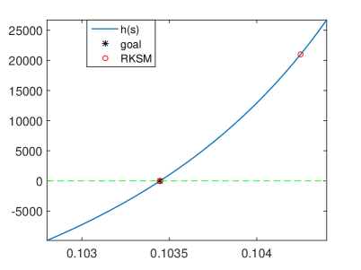
(a) $h(s)$

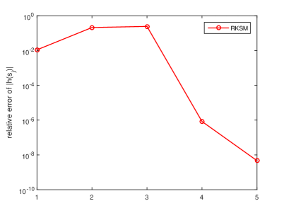
(b) $\frac{|h(s_{j})|}{\|x\|^{2}_{2}}$

In the left plot, the black asterisk denotes $(s_{*;1},h(s_{*;1}))$ and the red circle denotes the shifts $(s_{j},h(s_{j}))(j=3,4,5)$. As both $s_{1}$ and $s_{2}$ are outside the interval, they disappear. The right shows the convergence of $|h(s_{j})|$ to $0$.

4.2 Comparison with other algorithms

In this subsection, we test several algorithms for large-scale problems. Particularly, we compare RKSM with six algorithms: BN [34], PsdLcp [30], SDPT3 [28, 29], SeDuMi [26], cvx [13, 14] and LCPvA [35]. BN is a Newton type method for $h(s)=0$, and LCPvA is a projection method [35] in a similar framework as RKSM. Both SDPT3 and SeDuMi, which have been included in the package cvx, are designed for general semidefinite-quadratic-linear programming. The procedure of transforming an $\operatorname{SOCLCP}({\mathbb{K}}^{n},M,\boldsymbol{q})$ into a proper programming for cvx is given in [26], [28, Section 4.6] and [35, Appendix]. With $M=R^{\operatorname{T}}R$, the inputs for SDPT3 and SeDuMi are $R$ and $\boldsymbol{q}$, whereas the inputs of cvx are $M$ and $\boldsymbol{q}$. In all the experiments, the CPU times of forming $M$ or $R$ are not counted in.

The settings of parameters in algorithms, except for RKSM, are the same as the ones in [35]; for RKSM, we set $\epsilon_{1}=10^{-7}$ and $\epsilon_{2}=10^{-8}$ for the stopping criterion. Matrices of the following Example 2 and Example 3 are the same as [35, Section 7.2]. Due to version updating of some algorithms, performances of relevant algorithms change slightly.

In our reported results, “–” means either the failure of obtaining a solution within given stopping criterion, or returning a solution with $\chi_{\operatorname{rel}}>1e-1$, where $\chi_{\operatorname{rel}}$ is defined by (3.10). The label $d_{M}$ denotes the sparse densities of $M$; “# iter” represents the number of iterations, and “CPU(s)” reports the output of Matlab cputime. For our RKSM, “# iter” represents the dimension of the final subspace defined as

final dimension $$= + \ell \times j$$ dimension of initial subspace iteration number (4.2)

In this subsection, our initial subspace is set as ${\cal K}_{10,10}^{\operatorname{ext}}(J_{n}M,J_{n}\boldsymbol{q})$.

Example 2. This example is the same as [35, Table 7.3]. In [35], it reports average numbers of 4 results from 5 random examples. Here, we only present one result. The data matrix $M$ is again formed by $M=R^{\operatorname{T}}R,$ where $R$ is defined by (4.1) with $\texttt{n}=10000,\texttt{desity}=0.0005$. The condition number of $M$ is about $(\frac{1}{\texttt{rc}})^{2}$ and can range from $10^{2}$ to $10^{5}$. Results obtained from different kinds are listed in Table 4.3, where PsdLcp is excluded as the storage is out of memory.

Table 4.3: Numerical results of Example 2.

		kind=$1$			kind=$2$
	$\left(\frac{1}{\texttt{rc}}\right)^{2}(\approx\texttt{cond})$	$10^{2}$	$10^{4}$	$10^{5}$	$10^{2}$	$10^{4}$	$10^{5}$
	$d_{M}$	$7.3e\!-\!04$	$7.4e\!-\!04$	$7.5e\!-\!04$	$2.6e\!-\!03$	$2.6e\!-\!03$	$2.6e\!-\!03$
# iter	BN	$9/4$	$9/4$	$9/4$	$13/2$	$6/5$	$4/9$
	SDPT3	$22$	$19$	$21$	$15$	$19$	$21$
	Sedumi	$16$	$18$	$16$	$14$	$19$	$20$
	cvx	$19$	$21$	$22$	$12$	$15$	$18$
	LCPvA	$30$	$30$	$30$	$30$	$50$	$50$
	RKSM($\ell=1$)	$22$	$22$	$22$	$22$	$23$	$24$
	RKSM($\ell=10$)	$40$	$40$	$40$	$40$	$50$	$50$
CPU(s)	BN	$61.4$	$60.7$	$60.1$	$112.9$	$115.4$	$173.2$
	SDPT3	$1.23$	$1.03$	$1.75$	$57.8$	$72.0$	$80.4$
	Sedumi	$1.10$	$1.17$	$1.11$	$516.3$	$718.3$	$770.9$
	cvx	$4.17$	$2.90$	$1.76$	$2232.5$	$2611.7$	$3364.6$
	LCPvA	$0.14$	$0.15$	$0.15$	$39.6$	$61.9$	$67.4$
	RKSM($\ell=1$)	0.10	0.09	0.09	23.9	30.3	36.2
	RKSM($\ell=10$)	$0.12$	$0.11$	$0.12$	$38.9$	$52.1$	$52.4$
$\chi_{\operatorname{rel}}$	BN	$6.4e\!-\!12$	$7.3e\!-\!16$	$1.0e\!-\!13$	$6.1e\!-\!15$	$2.1e\!-\!14$	$1.2e\!-\!14$
	SDPT3	$1.9e\!-\!05$	$9.5e\!-\!05$	$1.2e\!-\!05$	$3.8e\!-\!08$	$2.3e\!-\!10$	$8.7e\!-\!09$
	Sedumi	$4.9e\!-\!07$	$8.4e\!-\!07$	$7.5e\!-\!07$	$9.3e\!-\!08$	$4.0e\!-\!09$	$2.6e\!-\!10$
	cvx	$4.8e\!-\!05$	$3.3e\!-\!07$	$1.3e\!-\!06$	$3.5e\!-\!08$	$1.6e\!-\!09$	$9.6e\!-\!12$
	LCPvA	$1.0e\!-\!12$	$9.7e\!-\!13$	$2.2e\!-\!13$	$8.4e\!-\!10$	$1.3e\!-\!11$	$6.0e\!-\!08$
	RKSM($\ell=1$)	$9.6e\!-\!11$	$1.1e\!-\!07$	$9.8e\!-\!08$	$1.4e\!-\!13$	$1.0e\!-\!11$	$5.7e\!-\!17$
	RKSM($\ell=10$)	$9.6e\!-\!11$	$1.1e\!-\!07$	$9.8e\!-\!08$	$1.4e\!-\!13$	$6.1e\!-\!17$	$2.2e\!-\!13$

From Table 4.3, we observe that RKSM converges fastest. For example, in 4 cases, RKSM($\ell=1$) uses $22$ iterations; since the dimension of the initial extended subspace is 20, this implies that RKSM($\ell=1$) computes $s_{*;1}$ in one iteration, and $s_{*;2}$ in another iteration. The similar discussion applies to RKSM($\ell=10$) when the “# iter” number is $40$ (i.e., $40=20+10\times 2$) by (4.2).

Example 3. This example is the same as [35, Table 7.4]. The tested $M\succ 0$ are from Matrix Market, and we do Cholesky decomposition $M=R^{\operatorname{T}}R$ and feed $R$ into SDPT3 and SeDuMi as inputs. The results are showed in Table 4.4.

Table 4.4: Numerical results of Example 3.

	$M$	s1rmq4m1	s1rmt3m1	s2rmq4m1	s2rmt3m1	s3rmq4m1	s3rmt3m1	s3rmt3m3	bcsstk17	bcsstk18
	$n$	$5489$	$5489$	$5489$	$5489$	$5489$	$5489$	$5357$	$10974$	$11948$
	$d_{M}$	$8.7e\!-\!03$	$7.2e\!-\!03$	$8.7e\!-\!03$	$7.2e\!-\!03$	$8.7e\!-\!03$	$7.2e\!-\!03$	$7.2e\!-\!03$	$3.6e\!-\!03$	$1.0e\!-\!03$
# iter	BN	$25/1$	$25/1$	$21/1$	$22/1$	$18/2$	$18/2$	$18/2$	$-$	$-$
	PsdLcp	$3$	$3$	$3$	$3$	$3$	$3$	$3$	$-$	$-$
	SDPT3	$15$	$16$	$14$	$13$	$12$	$18$	$14$	$19$	$31$
	Sedumi	$20$	$20$	$17$	$18$	$16$	$17$	$17$	$14$	$20$
	cvx	$20$	$20$	$18$	$18$	$16$	$15$	$16$	$11$	$19$
	LCPvA	$30$	$30$	$30$	$30$	$30$	$30$	$30$	$20$	$-$
	RKSM($\ell=1$)	$24$	$24$	$24$	$24$	$24$	$24$	$24$	$22$	$34$
	RKSM($\ell=10$)	$50$	$50$	$50$	$50$	$50$	$50$	$50$	$40$	$90$
CPU(s)	BN	$5.03$	$4.10$	$4.60$	$3.88$	$6.80$	$6.32$	$5.89$	$-$	$-$
	PsdLcp	$213.7$	$221.8$	$244.6$	$212.9$	$213.7$	$218.2$	$196.7$	$-$	$-$
	SDPT3	$14.38$	$14.3$	$12.6$	$11.7$	$11.1$	$16.4$	$326.0$	$30.2$	$243.2$
	Sedumi	$14.39$	$14.9$	$12.8$	$13.2$	$12.1$	$12.9$	$90.2$	$19.9$	$150.8$
	cvx	$20.0$	$16.5$	$27.1$	$16.3$	$18.3$	$8.20$	$6.50$	$11.2$	$14.5$
	LCPvA	$1.03$	$0.61$	$1.05$	$0.57$	$0.94$	$0.58$	$0.49$	$1.42$	$-$
	RKSM($\ell=1$)	0.83	0.51	0.82	0.51	0.83	0.53	0.45	0.72	1.89
	RKSM($\ell=10$)	$1.60$	$0.97$	$1.64$	$0.95$	$1.58$	$0.99$	$0.79$	$1.41$	$3.14$
$\chi_{\operatorname{rel}}$	BN	$1.1e\!-\!13$	$2.4e\!-\!13$	$1.8e\!-\!12$	$6.8e\!-\!12$	$1.5e\!-\!16$	$1.7e\!-\!17$	$1.1e\!-\!17$	$-$	$-$
	PsdLcp	$4.7e\!-\!14$	$7.8e\!-\!13$	$8.1e\!-\!13$	$1.8e\!-\!13$	$1.6e\!-\!09$	$2.3e\!-\!11$	$2.2e\!-\!10$	$-$	$-$
	SDPT3	$1.0e\!-\!06$	$4.8e\!-\!07$	$4.8e\!-\!08$	$9.4e\!-\!07$	$4.4e\!-\!07$	$3.8e\!-\!10$	$1.3e\!-\!07$	$1.5e\!-\!16$	$2.6e\!-\!14$
	Sedumi	$1.4e\!-\!08$	$1.4e\!-\!08$	$1.3e\!-\!09$	$7.7e\!-\!09$	$1.4e\!-\!07$	$5.6e\!-\!08$	$5.2e\!-\!08$	$4.8e\!-\!17$	$1.6e\!-\!15$
	cvx	$4.8e\!-\!05$	$3.1e\!-\!05$	$2.8e\!-\!06$	$4.3e\!-\!06$	$1.8e\!-\!06$	$1.5e\!-\!05$	$3.2e\!-\!07$	$3.1e\!-\!16$	$6.0e\!-\!09$
	LCPvA	$3.0e\!-\!09$	$4.0e\!-\!05$	$2.7e\!-\!09$	$1.0e\!-\!10$	$6.7e\!-\!10$	$1.2e\!-\!08$	$1.4e\!-\!09$	$5.3e\!-\!14$	$-$
	RKSM($\ell=1$)	$2.0e\!-\!10$	$1.4e\!-\!11$	$2.0e\!-\!10$	$1.3e\!-\!11$	$7.2e\!-\!11$	$1.3e\!-\!09$	$5.1e\!-\!09$	$2.4e\!-\!08$	$3.7e\!-\!09$
	RKSM($\ell=10$)	$6.1e\!-\!14$	$4.1e\!-\!14$	$1.6e\!-\!11$	$2.6e\!-\!12$	$3.5e\!-\!11$	$2.4e\!-\!10$	$6.1e\!-\!09$	$2.4e\!-\!08$	$2.7e\!-\!16$

We noticed that PsdLcp converges in only three iterations for most problems, but requires much more consuming time, mainly due to the full eigen-decompositions. LCPvA obtains a lucky break on bcsstk17 but cannot deal with bcsstk18, as reported in [35]. Due to a not good initial subspace, our RKSM($\ell=1$) spans a large subspace for bcsstk18 matrix $M$ with $\|M\|_{1}\approx 5.12\times 10^{10},\tau\approx 3.61\times 10^{3}$ and $s_{*}\approx 3.88\times 10^{3}$. A close check of RKSM($\ell=1$) indicates that the condition in line 7 is true, and thus the new shifts $s_{j}=\|M\|_{1}/10^{j}$ are used in line 8. Until at $j=7$ (i.e., $\|M\|_{1}/10^{7}\approx 5.12\times 10^{3}$), the condition in Line 7 becomes false and Line 10 is executed. Thus, the shifts are now near the target $s_{*}\approx 3.88\times 10^{3}$, and therefore, the subspace formed becomes good enough for ensuring the convergence of RKSM($\ell=1$).

By setting $\ell=10$ in RKSM for bcsstk18, the number of the ldl decompositions is reduced from 14 to 7, whereas the dimension of the final subspace increases from 34 to 90. In principal, it is possible to reduce the consuming CPU time as the callings of ldl decompositions decrease. However, due to the different efficiency of backslash and ldl for linear systems in Matlab, for bcsstk18, the reduced number of ldl decompositions is not enough to compensate the more expensive callings of ldl decomposition than backslash. The results are shown in Table 4.5. When the number of ldl calls for $\ell=1$ becomes sufficiently large, the reduced number (from using $\ell=10$) of ldl may compensate the extra consuming time of ldl, and we will see such an example in the flow problem in Example 4.

Table 4.5: CPU times of linear solvers for bcsstk18 in Example 3.

operation	$M\backslash\boldsymbol{q}$	ldl$(M)$	ldl$(M),M\backslash\boldsymbol{q}$	${\rm orth}\left[{\cal K}_{10}((J_{n}M)^{-1},(J_{n}M)^{-1}J_{n}\boldsymbol{q})\right]$
CPU(s)	$0.054$	$0.164$	$0.180$	$0.329$

Example 4. We test larger problems in which the associated matrices $M$ are from the benchmark[19] for model order reduction. In the field of dynamical systems, there involves many c-stable $A$, whose eigenvalues are all on left hand half plane. If c-stable $A$ is symmetric, then $A$ is negative positive definite. For those matrices, we simply take $M=-A$ as test matrices. The results are displayed in Table 4.6.

Table 4.6: Numerical results of Example 4.

	$M$	flow	rail5177	rail20209	gassensor	chip	t3dl	t2dal	t2dah
	$n$	$9669$	$5177$	$20209$	$66917$	$20082$	$20360$	$4257$	$11445$
	$d_{M}$	$7.2e\!-\!04$	$1.3e\!-\!03$	$3.4e\!-\!04$	$3.8e\!-\!04$	$7.0e\!-\!04$	$1.2e\!-\!03$	$8.7e\!-\!03$	$1.3e\!-\!03$
# iter	PsdLcp	$-$	$2$	$-$	$-$	$-$	$-$	$2$	$-$
	SDPT3	$23$	$-$	$-$	$-$	$21$	$-$	$-$	$-$
	Sedumi	$19$	$14$	$-$	$-$	$22$	$18$	$14$	$-$
	cvx	$18$	$-$	$-$	$-$	$-$	$-$	$-$	$-$
	LCPvA	$-$	$30$	$30$	$-$	$30$	$-$	$-$	$-$
	RKSM($\ell=1$)	$32$	$23$	$23$	$24$	$23$	$26$	$24$	$24$
	RKSM($\ell=10$)	$60$	$50$	$50$	$50$	$50$	$60$	$50$	$50$
CPU(s)	PsdLcp	$-$	$203.7$	$-$	$-$	$-$	$-$	$109.0$	$-$
	SDPT3	$1031.6$	$-$	$-$	$-$	$1025.0$	$-$	$-$	$-$
	Sedumi	$25.6$	$146.2$	$-$	$-$	$741.3$	$901.2$	$1.98$	$-$
	cvx	$6.30$	$-$	$-$	$-$	$-$	$-$	$-$	$-$
	LCPvA	$-$	$0.12$	$0.60$	$-$	$8.41$	$-$	$-$	$-$
	RKSM($\ell=1$)	$0.82$	0.09	0.44	85.0	5.96	$\scriptsize{18.3}$	0.14	0.57
	RKSM($\ell=10$)	0.76	$0.14$	$0.85$	$170.4$	$13.8$	$36.8$	$0.19$	$1.11$
$\chi_{\operatorname{rel}}$	PsdLcp	$-$	$3.6e\!-\!09$	$-$	$-$	$-$	$-$	$7.1e\!-\!10$	$-$
	SDPT3	$1.7e\!-\!10$	$-$	$-$	$-$	$7.3e\!-\!05$	$-$	$-$	$-$
	Sedumi	$4.5e\!-\!11$	$7.8e\!-\!04$	$-$	$-$	$8.6e\!-\!07$	$1.9e\!-\!08$	$8.6e\!-\!10$	$-$
	cvx	$6.1e\!-\!13$	$-$	$-$	$-$	$-$	$-$	$-$	$-$
	LCPvA	$-$	$1.4e\!-\!13$	$7.4e\!-\!12$	$-$	$1.9e\!-\!12$	$-$	$-$	$-$
	RKSM($\ell=1$)	$6.5e\!-\!08$	$7.6e\!-\!09$	$8.2e\!-\!09$	$5.8e\!-\!08$	$9.7e\!-\!09$	$3.6e\!-\!12$	$2.4e\!-\!16$	$1.3e\!-\!16$
	RKSM($\ell=10$)	$6.5e\!-\!08$	$3.6e\!-\!09$	$1.0e\!-\!10$	$1.7e\!-\!09$	$2.9e\!-\!09$	$6.0e\!-\!12$	$1.3e\!-\!09$	$1.0e\!-\!08$

We noted that BN fails in all these problems, and PsdLcp solves two medium cases. cvx successes in computing a solution within prescribed accuracy in only one example. By contrast, our RKSM works well for all these matrices. Also, for flow, we observed that RKSM($\ell=10$) needs slightly less CPU time than RKSM($\ell=1$) as the number of ldl decompositions is reduced from 12 to 4.

5 Conclusions

Following the framework of [35], in this paper, we proposed a new rational Krylov subspace method, RKSM($\ell$), for solving large-scale symmetric and positive definite $\operatorname{SOCLCP}({\mathbb{K}}^{n},M,\boldsymbol{q})$. Through a transformation of $\operatorname{SOCLCP}({\mathbb{K}}^{n},M,\boldsymbol{q})$ into a zero-finding equation, we first connect it with the transfer functions in the model reduction. According to the moment match theory in model reduction, we observed in Theorem 3.1 that the number of the matched moments for $h(s)$ doubles when $M$ is symmetric. Thus, with a strategy of using multiple approximations, we propose RKSM, which improves the convergence and robustness over [35] for the general $\operatorname{SOCLCP}({\mathbb{K}}^{n},M,\boldsymbol{q})$ with GUS property. Our numerical experiments demonstrate its efficiency and robustness.

References

- [1] N. Aliyev, P. Benner, E. Mengi, P. Schwerdtner, and M. Voigt, Large-scale computation of -norms by a greedy subspace method, SIAM J. Matrix Anal. Appl., 38 (2017), pp. 1496–1516.
- [2] A. C. Antoulas, Approximation of Large-Scale Dynamical Systems, Advances in Design and Control, SIAM, Philadelphia, PA, 2005.
- [3] Z. Bai and Y. Su, Dimension reduction of large-scale second-order dynamical systems via a second-order Arnoldi method, SIAM J. Sci. Comput., 25 (2005), pp. 1692–1709.
- [4] J.-S. Chen and S. H. Pan, A descent method for a reformulation of the second-order cone complementarity problem, J. Comput. Appl. Math., 213 (2008), pp. 547–558.
- [5] J.-S. Chen and P. Tseng, An unconstrained smooth minimization reformulation of the second-order cone complementarity problem, Math. Program., 104 (2005), pp. 293–327.
- [6] X. D. Chen, D. F. Sun, and J. Sun, Complementarity functions and numerical experiments on some smoothing Newton methods for second-order-cone complementarity problems, Comput. Optim. Appl., 25 (2003), pp. 39–56.
- [7] R. W. Cottle, J.-S. Pang, and R. E. Stone, The Linear Complementarity Problem, Computer Science and Scientific Computing, Academic Press, Inc., Boston, MA, 1992.
- [8] J. W. Demmel, Applied Numerical Linear Algebra, SIAM, Philadelphia, PA, 1997.
- [9] P. Feldman and R. W. Freund, Efficient linear circuit analysis by Padé approximation via the Lanczos process, IEEE Trans. Computer-Aided Design, 14 (1995), pp. 639–649.
- [10] M. Fukushima, Z.-Q. Luo, and P. Tseng, Smoothing functions for second-order-cone complementarity problems, SIAM J. Optim., 12 (2002), pp. 436–460.
- [11] K. Gallivan, E. Grimme, and P. Van Dooren, Asymptotic waveform evaluation via a Lanczos method, Appl. Math. Lett., 7 (1994), pp. 75–80.
- [12] G. H. Golub and C. F. Van Loan, Matrix Computations, Johns Hopkins University Press, Baltimore, Maryland, 4th ed., 2013.
- [13] M. Grant and S. Boyd, Graph implementations for nonsmooth convex programs, in Recent Advances in Learning and Control, V. Blondel, S. Boyd, and H. Kimura, eds., Lecture Notes in Control and Information Sciences, Springer-Verlag Limited, 2008, pp. 95–110.
- [14] , CVX: Matlab software for disciplined convex programming, version 2.1, Mar. 2014.
- [15] S. Hayashi, N. Yamashita, and M. Fukushima, A combined smoothing and regularization method for monotone second-order cone complementarity problems, SIAM J. Optim., 15 (2005), pp. 593–615.
- [16] , Robust Nash equilibria and second-order cone complementarity problems, 6 (2005), pp. 283–296.
- [17] R. A. Horn and C. R. Johnson, Matrix Analysis, cambridge university press, New York, NY, 2nd ed., 2013.
- [18] L. Knizhnerman and V. Simoncini, Convergence analysis of the extended Krylov subspace method for the Lyapunov equation, Numer. Math., 118 (2011), pp. 567–586.
- [19] J. G. Korvink and E. B. Rudnyi, Oberwolfach benchmark collection, in Dimension Reduction of Large-Scale Systems, P. Benner, D. C. Sorensen, and V. Mehrmann, eds., Berlin, Heidelberg, 2005, Springer Berlin Heidelberg, pp. 311–315.
- [20] D. Kressner and B. Vandereycken, Subspace methods for computing the pseudospectral abscissa and the stability radius, SIAM J. Matrix Anal. Appl., 35 (2014), pp. 292–313.
- [21] R.-C. Li and Z. Bai, Structure-preserving model reduction using a Krylov subspace projection formulation, Comm. Math. Sci., 3 (2005), pp. 179–199.
- [22] R.-C. Li and Q. Ye, Simultaneous similarity reductions for a pair of matrices to condensed forms, Comm. Math. Stat., 2 (2014), pp. 139–153.
- [23] W. H. A. Schilders, H. A. van der Vorst, and J. R. (editors), Model Order Reduction: Theory, Research Aspects and Applications, Springer, Boston, 2008.
- [24] V. Simoncini, A new iterative method for solving large-scale Lyapunov matrix equations, SIAM J. Sci. Comput., 29 (2007), pp. 1268–1288.
- [25] V. Simoncini, D. B. Szyld, and M. Monsalve, On two numerical methods for the solution of large-scale algebraic Riccati equations, IMA J. Numer. Anal., 34 (2014), pp. 904–920.
- [26] J. F. Sturm, Using SeDuMi 1.02, a MATLAB toolbox for optimization over symmetric cones, vol. 11/12, 1999, pp. 625–653. Interior point methods.
- [27] T.-J. Su and J. R. R. Craig, Model reduction and control of flexible structures using Krylov vectors, J. Guidance, Control, and Dynamics, 14 (1991), pp. 260–267.
- [28] K.-C. Toh, M. J. Todd, and R. H. Tütüncü, On the implementation and usage of SDPT3—a Matlab software package for semidefinite-quadratic-linear programming, version 4.0, in Handbook on semidefinite, conic and polynomial optimization, vol. 166 of Internat. Ser. Oper. Res. Management Sci., Springer, New York, 2012, pp. 715–754.
- [29] R. H. Tütüncü, K. C. Toh, and M. J. Todd, Solving semidefinite-quadratic-linear programs using SDPT3, vol. 95, 2003, pp. 189–217. Computational semidefinite and second order cone programming: the state of the art.
- [30] X. Wang, X. Li, L.-H. Zhang, and R.-C. Li, An efficient numerical method for the symmetric positive definite second-order cone linear complementarity problem, J. Sci. Comput., 79 (2019), pp. 1608–1629.
- [31] W. H. Yang and X. M. Yuan, The GUS-property of second-order cone linear complementarity problems, Math. Program., 141 (2013), pp. 295–317.
- [32] W. H. Yang, L.-H. Zhang, and C. Shen, On the range of the pseudomonotone second-order cone linear complementarity problem, J. Optim. Theory Appl., 173 (2017), pp. 504–522.
- [33] L.-H. Zhang and W. H. Yang, An efficient algorithm for second-order cone linear complementarity problems, Math. Comp., 83 (2013), pp. 1701–1726.
- [34] , An efficient matrix splitting method for the second-order cone complementarity problem, SIAM J. Optim., 24 (2014), pp. 1178–1205.
- [35] L.-H. Zhang, W. H. Yang, C. Shen, and R.-C. Li, A Krylov subspace method for large scale second order cone linear complementarity problem, SIAM J. Sci. Comput., 37 (2015), pp. A2046–A2075.
- [36] Y. Zhou and R.-C. Li, Bounding the spectrum of large Hermitian matrices, Linear Algebra Appl., 435 (2011), pp. 480–493.