Coronal Elemental Abundance: New Results from Soft X-ray Spectroscopy of the Sun

1 Introduction

S-Introduction

The abundance of elements in the solar photosphere is well established from many decades of systematic observations of the Sun using a variety of techniques and this has resulted in high confidence photospheric abundance values. However, abundance studies in the solar corona and coronae of other stars, have not kept pace compared to photospheric studies. Though it is widely believed that there exists a steady flow of photospheric material into the corona, possibly channelled by structures associated with magnetic field configurations, the coronal abundance shows distinct deviations from photospheric values. For the solar case, studies show enhanced abundance of elements with low first ionisation potential (FIP) over photospheric values, often categorized as a FIP bias (ratio of low FIP element coronal abundances to corresponding photospheric values). Stellar coronae also exhibit this effect (Drake, Laming, and Widing, 1997; Laming and Drake, 1999; Garcia-Alvarez et al., 2004) as well as the inverse termed as inverse-FIP (IFIP) effect (see Laming, 2015, for a review). Studies in the past such as those by Feldman (1992), Fludra and Schmelz (1999), Phillips et al. (2003), Feldman and Laming (2006), Sylwester et al. (2010), Sylwester et al. (2012), Schmelz et al. (2012), Narendranath et al. (2014), Dennis et al. (2015) and Moore et al. (2018) to name a few, suggest that this deviation or FIP bias is not the same for all elements. The range of reported values in the past, also suggests that FIP bias values may be nominally stable but possibly vary with solar cycle phase (Brooks et al., 2017) and spatial location on the Sun.

The first result on the spectroscopic measurements of FIP bias variability during the evolution of a flare was provided by Sylwester, Lemen, and Mewe (1984). Ca abundances measured by the Rentgenovsky Spektrometr s Izognutymi Kristalami (RESIK) Bragg Crystal spectrometer were observed to increase as the flux in the narrow band continuum increased and showed a hysteresis during the decay of the flare. Flare to flare differences in Ca abundance were presented in further detail by Sylwester et al. (1998). Warren (2014) measured the Fe abundances (from irradiance measurements) using the Extreme Variability Experiment (EVE) on board the Solar Dynamics Observatory (SDO) at the peak of strong flares (X and M) showing that the plasma has photospheric compositions. Measurements from the Flat Crystal Spectrometer (FCS) of the Soft X-rays Polychromator on board the Solar Maximum Mission (SMM) showed large variations in abundances even within non-flaring active regions and bright points of the quiescent Sun (Saba and Strong, 1994).

Recent studies are providing evidence that suggest the key role of local magnetic fields in generating the observed FIP bias. A detailed study of an active region by Baker et al. (2015) reports a decrease in FIP bias (abundances close to photospheric) that is linked to small scale evolution of the underlying magnetic field. FIP bias in emerging flux regions in a coronal hole were studied by Baker et al. (2018) and it was shown that the changes were related to the magnetic topology of the regions. Baker et al. (2019) observed IFIP patches at the foot points during two confined flares in an active region and Baker et al. (2020) reported similar observations in a highly complex active region with multiple strong flares. Over solar cycle time scales, Brooks et al. (2017) showed a strong correlation of Ne coronal to photospheric abundance ratios, to the phases of the solar cycle. Pipin and Tomozov (2018) further extended this to stars and have shown that the FIP bias variations are likely related to the large scale coronal magnetic field and activity level of the toroidal magnetic field. Such variations could also occur at shorter time scales and smaller spatial scales. Laming (2017) presented scenarios where the dependence of the variations in FIP bias is linked to the origin and propagation sites of Alfvén waves.

Variations in coronal abundances in stellar flares have also been observed in quiescent coronae which are IFIP biased showing photospheric composition during those flares (Nordon, R. and Behar, E., 2008; Laming and Hwang, 2009; Sasaki et al., 2020).

In this work, we provide clear evidence for FIP bias variation during the evolution of flares at short time scales (minutes to seconds). While our flare averaged abundance values are within the range reported earlier, this work systematically probes the variation of FIP bias of Si, S, Ca, and Fe, during the course of individual flares as well as their variations across flare classes.

2 Observations

sec:obs

Soft X ray spectroscopy of the solar corona is a useful diagnostic to remotely study the plasma composition and its changes over time. Crystal-based X-ray spectrometers have derived abundances using (line plus continuum) measurements in narrow spectral bands with high resolution and centered about the line of interest. Ideally, X-ray spectra below 8 keV need to be measured simultaneously with the continuum to clearly derive plasma temperature and accurate estimates of X-ray line flux. Non-imaging broad band solar soft X-ray spectrometers have been flown as supporting instruments in many planetary missions since a knowledge of the rapidly evolving solar X-ray spectra is required to convert planetary X ray flux to elemental abundances. We used data from three missions with similar spectrometers (Si-PIN diodes) to derive elemental abundances of the corona during a range of solar activity levels.

2.1 SMART-1 XSM

The X-ray Solar Monitor (XSM) on the Small Missions for Advanced Research in Technology-1 (SMART-1) (Huovelin et al., 2002) is a single pixel, non imaging Si-PIN detector with a 105^∘ full field of view such that the full disk of the Sun is observed at nearly all times. The solar data from this mission spans from 03 March 2004 to 30 August 2006 which includes the Earth escape phase and lunar orbit phase when the solar activity was low. The useful operational energy range was $\approx$ 2 keV to 20 keV with some exceptions where the lower energy threshold comes down to 1.8 keV (Si abundances were derived only for such cases). We have used spectral data of nine long duration flares for this work which fall in the B-C class.

2.2 Chandrayaan-1 XSM

The X-ray Solar Monitor on Chandrayaan-1 is similar to the SMART-1 XSM except for a reduction in the aperture size to accommodate a wider dynamic range in the expected counts. This instrument measured the X-ray spectrum in the range of approximately 1.8 - 20 keV from several X-ray flares during the nine month mission life from 28 November 2008 to 29 August 2009 and the results were presented in Narendranath et al. (2014). Narendranath et al. (2014). Here we have used a C1 flare from XSM to look at the variation in FIP bias during the latter.

2.3 MESSENGER- SAX

The Solar X ray Assembly (SAX) onboard the Mercury Surface, Space Environment, Geochemistry and Ranging (MESSENGER) satellite (around Mercury) observed the Sun in X-rays during the period from 2004 to 2014. The observations at the distance of Mercury began in 2007. We have chosen 33 flares in the B-M class for this work which have a clean rise and decay profile. The spectral resolution of SAX is 600 eV at 5.9 keV with which the X-ray emission lines of Si, S and Ca are not well resolved. However as shown by Dennis et al. (2015), in the 1.6 to 4 keV region dominated by line emission, good fits do provide a measure of the elemental abundances.

3 Analysissec:analysis

The XSMs measure solar spectra with a time resolution of 16 s while SAX spectra have typically 300 s binning. Since a range of activity levels are covered, we used different integration times, suitably adjusted for the strength of flares. The integrated flux (photons/cm²/s) in the 2 - 10 keV band multiplied by the integration time is taken as a measure of the strength of the flare for inter-flare comparison. SAX has a flat spectral resolution of 600 eV across its energy range while energy dependent resolution is incorporated for the XSMs. On board radioactive sources help in the calibration of XSMs and response matrices with temperature dependent corrections for each data set are generated.

The spectral analysis was carried out with the Object Spectral Executive (OSPEX) package which comes as part of the standard solarsoft package (SSW) Freeland and Handy (1998). The spectra were fitted with a thermal model (single temperature) calculated from CHIANTI (version 8.0.2) Dere et al. (1997) (vth$\_$abund in OSPEX) which consists of a continuum and multiple emission lines. For larger flares, we added a non-thermal component to fit the continuum (thick2 in OSPEX). Sample spectral fits from SMART-1 XSM, Chandrayaan-1 XSM and MESSENGER-SAX are shown in figure spec. All three instruments are Si-PIN detectors that do not have any significant continuum background. In the absence of X-ray events, the background appears only as a peak at the lower channels. This is not the same for all detectors and varies with the leakage current. We have taken intervals where the leakage current is less than 10 pA for all three detectors which ensures a more stable performance. The X-ray emission measured is for the whole solar disc. We subtracted the pre-flare spectrum to ensure that the derived abundances are indeed of the flare plasma. Elemental abundances were derived in the usual logarithmic ratio with respect to hydrogen (A_elem = log(N_elem/N_H + 12.0). The FIP bias values were derived with respect to the photospheric abundances as given in Asplund et al. (2009). Error bars are uncertainties arising from propagation of errors of fit parameters, while expressing it as a ratio to photospheric values (or FIP bias). The Fe line is excited only at higher plasma temperatures and is weak when temperatures are lower as in smaller flares.

Table 1.: Data source instruments tab:inst.

T-simple Instrument Energy range Spectral Time Obs.period Resolution Resolution SMART-1-XSM 1.8 to 20 keV 280 eV 16 s 3/03/04 to 30/08/06 Chandrayaan-1-XSM 1.8 to 20 keV 220 eV 16 s 28/11/08 to 29/08/09 MESSENGER-SAX 1.6 to 9.5 keV 600 eV 300 s 2007 to 2014

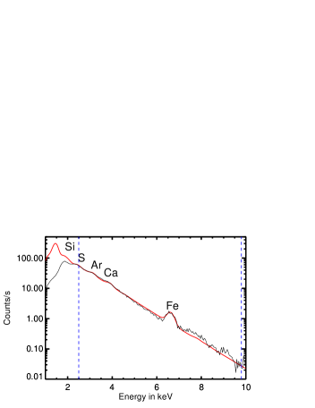
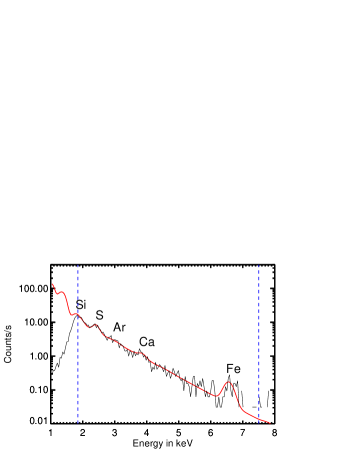
                       (a)                               (b)

  

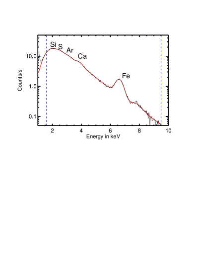
                                           (c)

Figure 1.: Representative spectral fits to flare spectrum from (a) SMART-1 XSM (26 June 2004) (b) Chandrayaan-1 XSM (5 July 2009) (c) MESSENGER SAX (2 January 2014). The red line indicates the best fit model (single temperature plasma varying the abundances) and the black line shows the data. Emission lines from elements are marked at expected line energies. Vertical blue dotted lines indicate the energy range used for fitting the model to the spectrum. spec

4 FIP Bias

sec:fip FIP bias has been reported in the solar corona for several decades now. We have measured the abundances of low FIP elements Si, Ca and Fe, the mid-FIP element S and the high-FIP element Ar during 43 flares using full disk integrated spectra. Individual flares which are isolated events that dominate the soft X-ray emission over the entire solar disk, are analysed in detail.

Figures FIP_var_1, FIP_var_2, and FIP_var_3 show the evolution of FIP bias values for each of the four low FIP elements as a function of time along with integrated light curves in the 2 - 10 keV range for three independent flares. Ar abundances derived have higher uncertainties in comparison to the low FIP elements and hence are not shown here. The FIP bias value of low FIP elements systematically decreases as the flare intensity rises to a maximum and the bias value shows clear and consistent evidence for recovery as the flare decays. For example, in Figure  FIP_var_1d, Fe FIP bias decreases from around 4 to 1.4 and recovers to 4 after the flare. Si in Figure  FIP_var_2a decreases to 1 from a preflare value of about 5. Ca FIP bias varies between 5 - 1 and does not show clear higher pre-flare values.

The FIP bias of S varies from 2.5 during pre- and post-flares to 1 during the flare phase. These variations are significantly beyond the error bars within the observation interval but are less when compared to other elements. This behavior of FIP bias during a flare is independently shown by each of the low-FIP elements detected in the multiple spectra. However, recovery to pre-flare values is not clearly visible in complex flaring events. For example, in Figure FIP_var_3 where this could arise due to sustained outburst lasting more than an hour with multiple re-connection events.

Date	UTC	GOES	Temperature	Si	S	Ca	Fe	Flux (2-10 keV)
		class(approx)	(MK)					in photons/cm2/s
17.04.04	04:46:00 to 05:05:52	B3	9.46$\pm$0.48	0.40$\pm$0.26	0.29$\pm$0.12	1.12$\pm$0.85	4.27$\pm$0.39	192098.8
01.05.04	04:30:32 to 05:40:40	B9	10.12$\pm$0.08	3.89$\pm$0.27	0.17$\pm$0.06	0.92$\pm$0.19	5.76$\pm$0.87	344738.7
05.05.04	19:27:04 to 20:04:24	B1	9.73$\pm$ 0.15	2.37$\pm$1.66	0.14$\pm$0.11	2.04 $\pm$ 0.36	5.37 $\pm$ 1.98	680821.6
22.05.04	06:46:32 to 07:51:52	C1	9.47 $\pm$0.11	3.75$\pm$0.43	2.76 $\pm$0.33	4.46$\pm$0.85	8.53$\pm$1.50	687424.6
24.05.04	10:56:08 to 11:50:00	C3	14.76$\pm$0.04	0.41$\pm$0.04	0.50$\pm$0.04	1.52$\pm$ 0.13	0.54$\pm$0.05	2790486.5
26.06.04	02:50:59 to 03:13:23	B2	7.80$\pm$0.05	0.39$\pm$0.06	0.27$\pm$0.03	0.92$\pm$0.16	8.51$\pm$1.45	351884.7
05.07.04	05:14:11 to 05:41:39	A3	6.17$\pm$0.10	0.39$\pm$0.32	0.67$\pm$0.41	4.25$\pm$1.59	8.44$\pm$1.27	50387.25
02.01.05	05:14:11 to 05:41:39	C1	10.37$\pm$0.32	4.28$\pm$0.51	1.74$\pm$0.28	0.42$\pm$0.23	8.53$\pm$1.71	199968.3
02.05.05	05:23:28 to 05:54:46	C	10.38$\pm$0.05	0.39$\pm 0.05$	0.14$\pm$0.02	1.59$\pm$0.13	0.55$\pm$0.07	2833431.5
05.07.09	08:58:05 to 09:23:09	A8	4.96$\pm$0.10	3.89$\pm$0.27	0.81$\pm$0.10	1.54$\pm$0.61	4.27$\pm$0.39	40390.7
02.01.14	01:52:44 to 06:57:24	M1	12.70$\pm$0.14	2.01$\pm$0.19	1.41$\pm$0.12	4.31$\pm$0.39	3.12$\pm$ 0.36	2187142.0
04.01.14	10:04:47 to 12:28:07	M	13.09$\pm$0.09	2.87$\pm$0.28	1.70$\pm$ 0.16	3.78$\pm$0.41	3.06$\pm$ 0.31	717274.6
04.01.14	21:48:07 to 00:01:27	M1	15.38 $\pm$ 0.05	1.93$\pm$ 0.16	1.37$\pm$ 0.11	4.56$\pm$ 0.36	1.83$\pm$0.17	5996155.5
17.01.14	03:32:57 to 06:29:37	C2	10.23$\pm$ 0.16	3.77$\pm$ 0.41	2.40$\pm$ 0.25	3.97$\pm$ 0.54	8.38$\pm$ 1.38	568340.4
17.01.14	18:59:37 to 21:19:37	C8	12.18 $\pm$ 0.33	1.96$\pm$ 0.33	1.80$\pm$ 0.21	4.02$\pm$ 0.44	3.52$\pm$ 0.67	2290718.3
18.01.14	02:16:29 to 03:13:09	B7	12.03 $\pm$ 0.16	2.69$\pm$ 0.26	2.08$\pm$ 0.20	3.44$\pm$ 0.48	5.42$\pm$ 0.83	1316521.5
18.01.14	03:23:09 to 04:19:49	C1	10.13 $\pm$ 0.12	2.64$\pm$ 0.26	2.00$\pm$ 0.19	1.89$\pm$ 0.45	8.39$\pm$ 1.36	618368.5
18.01.14	04:39:49 to 06:19:49	C	12.92$\pm$ 0.12	2.39$\pm$ 0.21	1.34$\pm$ 0.12	2.55$\pm$ 0.33	4.77$\pm$ 0.57	1925846.6
18.01.14	10:40:29 to 11:53:49	C2	9.97$\pm$ 0.10	2.70$\pm$ 0.32	1.83$\pm$ 0.21	3.01$\pm$ 0.51	8.48$\pm$ 1.31	597014.6
18.01.14	13:13:49 to 16:40:29	-	12.10$\pm$ 0.31	4.23$\pm$ 0.40	2.39$\pm$ 0.24	3.14$\pm$ 0.48	8.48$\pm$ 2.07	642723.6
18.01.14	19:40:29 to 21:03:49	C1	9.56 $\pm$ 0.13	4.35$\pm$ 0.44	2.71$\pm$ 0.27	3.34$\pm$ 0.60	8.52$\pm$ 1.53	417767.7
20.01.14	02:23:55 to 03:47:15	C2	9.31$\pm$ 0.13	2.53$\pm$ 0.23	2.12$\pm$ 0.19	3.66$\pm$ 0.56	8.18$\pm$ 1.60	413894.8
20.01.14	06:30:35 to 07:57:15	C1	9.58$\pm$ 0.13	3.22$\pm$ 0.31	2.12$\pm$ 0.20	1.55$\pm$ 0.41	8.53$\pm$ 1.51	402487.6
20.01.14	14:41:15 to 16:37:65	-	11.66 $\pm$ 0.10	3.49$\pm$ 0.29	2.48$\pm$ 0.23	5.13$\pm$ 0.51	5.42$\pm$ 0.65	1603430.0
20.01.14	21:41:15 to 00:04:35	C3	9.77$\pm$ 0.13	4.62$\pm$ 0.59	2.76$\pm$ 0.38	4.73$\pm$ 0.87	8.47$\pm$ 1.21	1089878.4
27.01.14	02:14:21 to 03:31:01	-	9.47 $\pm$ 0.11	3.75$\pm$ 0.43	2.76$\pm$ 0.33	4.46$\pm$ 0.85	8.53$\pm$ 1.50	687424.6
27.01.14	07:54:21 to 09:21:01	C4	11.52$\pm$ 0.10	3.19$\pm$ 0.28	1.66$\pm$ 0.15	4.80$\pm$ 0.54	7.48$\pm$ 0.94	1317998.3
27.01.14	12:54:21 to 14:17:41	-	9.11$\pm$ 0.15	3.09 $\pm$ 0.36	2.17$\pm$ 0.23	3.15$\pm$ 0.70	8.44$\pm$ 2.11	281918.9
27.01.14	18:28:21 to 20:18:21	C8	13.32$\pm$ 0.24	4.00$\pm$ 0.47	2.75$\pm$ 0.25	6.97$\pm$ 0.71	3.53$\pm$ 0.50	1445175.0
27.01.14	20:25:01 to 21:35:01	C5	12.28$\pm$ 0.18	2.92$\pm$ 0.33	2.22$\pm$ 0.20	6.17$\pm$ 0.63	3.48$\pm$ 0.48	1644204.9
27.01.14	22:12:58 to 23:57:58	M4	13.46$\pm$ 0.76	1.86$\pm$ 0.56	1.63$\pm$ 0.33	4.55$\pm$ 0.55	2.37$\pm$ 0.68	3465951.0
28.01.14	07:12:00 to 08:24:33	M3	20.12$\pm$ 0.83	6.40$\pm$ 0.81	2.73$\pm$ 0.32	5.84$\pm$ 0.83	3.10$\pm$ 0.54	2514868.8
28.01.14	21:48:55 to 23:88:55	M1	15.04$\pm$ 0.24	2.56$\pm$ 0.27	1.43$\pm$ 0.15	4.21$\pm$ 0.39	2.14$\pm$ 0.24	4676428.0
02.02.14	01:04:38 to 01:34:38	C6	13.00$\pm$ 0.24	3.49$\pm$ 0.46	2.28$\pm$ 0.23	4.99$\pm$ 0.62	4.62$\pm$ 0.67	1625441.1
02.02.14	02:50:38 to 03:33:58	C2	11.02$\pm$ 0.17	2.04$\pm$ 0.29	1.87$\pm$ 0.21	4.05$\pm$ 0.58	4.98$\pm$ 0.87	938765.5
02.02.14	08:00:38 to 09:07:18	M1	16.39 $\pm$ 0.46	3.50$\pm$ 0.59	2.60$\pm$ 0.30	5.81$\pm$ 0.55	1.42$\pm$ 0.17	7493439.5
02.02.14	11:29:17 to 12:35:57	C9	12.75$\pm$ 0.43	3.21$\pm$ 0.76	2.70$\pm$ 0.41	3.94$\pm$ 0.83	3.53$\pm$ 0.69	1263622.6
02.02.14	14:02:37 to 15:25:57	C8	13.39 $\pm$ 0.31	5.15$\pm$ 0.70	2.76$\pm$ 0.30	5.46$\pm$ 0.69	4.36$\pm$ 0.65	1790274.3
02.02.14	16:09:17 to 17:29:17	M	12.92 $\pm$ 0.34	4.88$\pm$ 0.77	2.76$\pm$ 0.34	6.20$\pm$ 0.78	5.07$\pm$ 0.81	1409684.5
06.02.14	03:56:47 to 05:20:07	C6	12.10$\pm$ 0.10	1.74$\pm$ 0.16	1.25$\pm$ 0.10	2.98$\pm$ 0.31	3.10$\pm$ 0.34	1856722.6
07.02.14	04:43:27 to 05:26:47	M1	14.54 $\pm$ 0.13	1.94$\pm$ 0.19	1.76$\pm$ 0.15	3.99$\pm$ 0.36	1.67$\pm$ 0.17	5151088.5
09.02.14	15:28:04 to 17:34:44	M	12.31 $\pm$ 0.10	2.01$\pm$ 0.18	1.60$\pm$ 0.13	3.45$\pm$ 0.31	2.42$\pm$ 0.25	2960934.5
12.02.14	00:05:59 to 00:06:46	-	8.86 $\pm$ 0.13	2.44$\pm$ 0.24	1.72$\pm$ 0.18	3.20$\pm$ 0.66	8.30$\pm$ 1.77	393868.4
09.09.14	00:10:30 to 03:10:30	M4	11.12$\pm$ 0.09	1.83$\pm$ 0.16	1.57$\pm$ 0.13	3.92$\pm$ 0.38	4.67$\pm$ 0.55	1228230.1

Table 2.: tab:BiasList of solar flares analysed in this study. The FIP bias values are given for all the low FIP elements in the spectral range studied. The flux is the integrated flux in the 2 to 10 keV band. Some of the flares seen in SAX MESSENGER were not observed in GOES and hence the GOES class not mentioned for those cases.

For flares with sharply defined peaks, the minimum of the FIP bias appears to precede the peak as shown in Figure all_bias. Additionally, there is a difference observed in the rate of recovery to coronal values.

We also studied FIP bias variations using the full set of 43 flares (Table 2). Data during the whole interval of a flare are summed and analysed, to derive the mean FIP bias for each flare. A dotted line is drawn at FIP bias value equal to 1 which is when coronal abundances equal photospheric values. The general trend for all elements of lower FIP bias for stronger flares (Figure FIP_flares), is consistent with the speculation in Katsuda et al. (2020) that more intense flares show larger departures of FIP values from nominal. Katsuda et al. (2020) used albedo signal from Earth’s atmosphere during four giant solar flares measured using the X-ray imaging spectrometer on Suzaku. Unlike our work, during the Suzaku observations, the flare spectrum was not continuously monitored to derive the rapidly changing FIP bias values with time, probably due to spacecraft constraints. Instead, bias values were compared from successive orbits with a large time gap of nearly 90 minutes to arrive at their conclusion. Our cumulative data for 43 flares show this trend most clearly for Fe, followed by Si. S is the least fractionated. The trend is not very evident for Ca even though the detailed analysis of individual flares, shows changes consistent with other low-FIP elements. This could arise from the fact that the data points in Figure FIP_flares represent mean FIP bias for the observed flare duration. In addition, Figure FIP_flares shows that Ca has a greater tendency for a quick recovery to pre-flare FIP bias values as the flare crosses its peak.

There are a few instances of FIP bias falling below photospheric values. Katsuda et al. (2020) also reports IFIP values for S and Si during the decay phase. We suggest that in the future this can be investigated in detail using a larger sample of flares and flare classes.

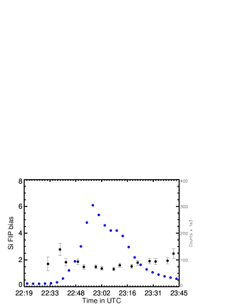
         (a)                               (b)

  

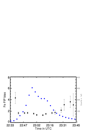
         (c)                               (d)

Figure 2.: Variation of FIP bias values during an M flare on 6 January 2014. (a) Si, (b) S, (c) Ca, and (d) Fe. The light curve of the flare in the 2-10 keV energy range is plotted in blue. FIP˙var˙1

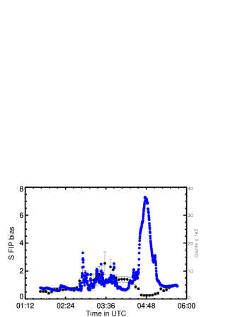
         (a)                                (b)

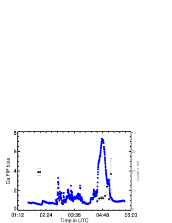
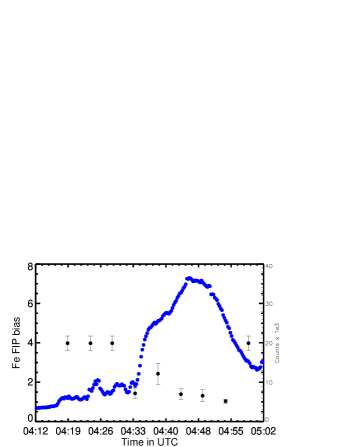
         (c)                                (d)

Figure 3.: Variation of FIP bias values during a B9 flare on 1 May 2004.(a) Si (b) S (c) Ca and (d) Fe. The light curve of the flare in the 2-10 keV energy range is plotted in blue. FIP˙var˙2

  

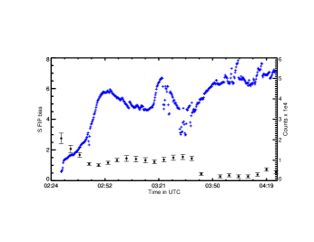
         (a)                                (b)

  

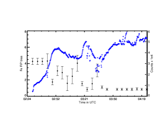
         (c)                                (d)

Figure 4.: Variation of FIP bias values during a C flare on 2 January 2005.(a) Si, (b) S, (c) Ca, and (d) Fe. The light curve of the flare in the 2-10 keV energy range is plotted in blue. FIP˙var˙3

  

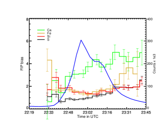
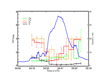
            (a)                                 (b)

Figure 5.: FIP bias variation for the flares on (a) 6 January 2014 ( data in Figure 3) (b) 1 May 2004 (data in figure 4) for Ca, Fe, Si and S . The light curve in the 2-10 keV energy range is plotted in blue. The recovery rates are observed to be different. all˙bias

  

  

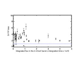
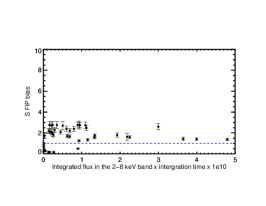
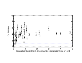
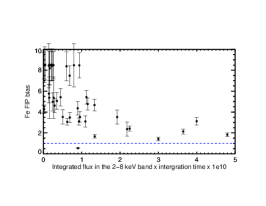
Figure 6.: FIP bias variations across flares as a function of the strength of the flare (integrated flux in the 2-10 keV multiplied by the integration time). The spectra during the whole interval of the flare are summed and analysed for 43 flares. The trend suggests a lower FIP bias (and lesser fractionation) for higher intensity flares. A dotted blue line is drawn at FIP bias value=1 which is when coronal abundances are equal to photospheric ones. FIP˙flares

5 Discussion

The coronal FIP bias, first reported by Pottasch (1963) and consistently reported in subsequent years by numerous authors is studied during flares using UV and X-ray spectroscopic techniques, through direct sampling in slow and fast solar wind and during observations of solar energetic events (SEP) in Earth’s vicinity. The degree of enhancement reported in these studies shows a large range.

Explanations for this long standing puzzle of enhancement of low FIP elemental abundance in the solar corona have been attempted by many authors. Currently, the FIP effect is understood as arising from fractionation in the chromosphere and subsequent acceleration of these ions in a force-free field into the corona. Theoretical frameworks are described in Hénoux (1998), Laming (2004), Laming (2009), Laming (2012), Laming (2015). Laming (2004) suggested a ponderomotive force arising from wave refraction in an inhomogenous plasma. In a magnetic plasma, waves with frequencies much lower than the ion cyclotron frequency are refracted to regions of high wave energy density taking along the ions producing the FIP effect.

Laming (2017) studied the dependence of fractionation of elements on the origin and propagation of Alfven waves through the chromosphere. The model reproduces the observed fractionations in both open and closed field regions. Laming et al. (2019) applied the model to investigate scenarios in source regions of SEPs and the solar wind.

The results from our study here shows the time dependent variation of FIP bias during the evolution of flares.

Soft X-ray emission in solar flares is dominant from the closed loops that are filled with hot plasma. One of the ways to understand the systematic reduction in FIP bias during the rising phase of a flare is the following. Assuming that a reconnection process leads to a flare, the pre-flare magnetic field configuration rapidly changes and new channels for upward flow may emerge. Plasma from the upper photosphere fills the coronal loops which are observed in X rays. The fractionation is brought about in the chromosphere by the action of the ponderomotive force. The possible scenarios and parameter dependence of such a model for variations in the degree of fractionation (as observed here) is described in Laming (2017). When the upward flow speeds of the plasma is high, it would pass through the chromosphere too quickly to get fractionated. During flares it is likely that the subtle variations in the FIP bias as observed here is indicative of the variations in heating and chromospheric evaporation.

After flare maximum, the field configuration in the lower corona recovers to form new closed shapes in loops that lead to reduced flow rates and higher fractionation.

Though Laming (2017) model is more suitable for quiet Sun conditions, the FIP bias decrease during a flare observed in this work can be attributed to the presence of an open field configuration during a reconnection process in active regions.

6 Summary

The evolution of absolute elemental abundances of Si, S, Ca, and Fe in the flare plasma has been determined from soft X-ray spectroscopy. We show that during flare peaks, the abundance of low FIP elements significantly reduces to photospheric values. Short time-scale variations in the abundance values observed in flares provide a framework to model the wave propagation and plasma heating during disturbed solar conditions. Future measurements extending down to 0.5 keV with high resolution spectrometers along with chromospheric velocity variation and magnetic field measurements during the evolution of a flare would provide valuable additional information to further constrain the model.

Acknowledgments

We thank Brian Dennis, Richard Schwartz, Kim Tolbert at GSFC and Vinay Kashyap at CFA for useful discussions under the Indo-US Science and Technology Forum. We extend our gratitude to IUSSTF grant JC-24-2015 for funding this research. We also very much appreciate the comments and suggestions from the anonymous reviewer that has helped us improve the paper.

Disclosure of Potential Conflicts of Interest: The authors declare that there are no conflicts of interest.

References

- Asplund et al. (2009) Asplund, M., Grevesse, N., Sauval, A.J., Scott, P.: 2009, The Chemical Composition of the Sun. Annu. Rev. Astron. Astrophys. 47, 481. DOI. ADS.
- Baker et al. (2019) Baker, D., van Driel-Gesztelyi, L., Brooks, D.H., Valori, G., James, A.W., Laming, J.M., Long, D.M., Démoulin, P., Green, L.M., Matthews, S.A., Oláh, K., Kővári, Z.: 2019, Transient Inverse-FIP Plasma Composition Evolution within a Solar Flare. Astrophys. J. 875, 35. DOI. ADS.
- Baker et al. (2020) Baker, D., van Driel-Gesztelyi, L., Brooks, D.H., Démoulin, P., Valori, G., Long, D.M., Laming, J.M., To, A.S.H., James, A.W.: 2020, Can subphotospheric magnetic reconnection change the elemental composition in the solar corona? Astrophys. J. 894, 35. DOI. https://doi.org/10.3847%2F1538-4357%2Fab7dcb.
- Brooks et al. (2017) Brooks, D.H., Baker, D., van Driel-Gesztelyi, L., Warren, H.P.: 2017, A Solar cycle correlation of coronal element abundances in Sun-as-a-star observations. Nat. Commun. 8, 183. DOI. ADS.
- Dennis et al. (2015) Dennis, B., Phillips, K., Schwartz, R., Tolbert, K., Starr, R., Nittler, L.: 2015, Solar flare element abundances from the solar assembly for x-rays (sax) on messenger. Astrophys. J. 803, 67. DOI.
- Dere et al. (1997) Dere, K.P., Landi, E., Mason, H.E., Monsignori Fossi, B.C., Young, P.R.: 1997, CHIANTI - an atomic database for emission lines. Astron. Astrophys. Suppl. Ser 125, 149. DOI. ADS.
- Drake, Laming, and Widing (1997) Drake, J.J., Laming, J.M., Widing, K.G.: 1997, Stellar Coronal Abundances. V. Evidence for the First Ionization Potential Effect in Centauri. Astrophys. J. 478, 403. DOI. ADS.
- Feldman (1992) Feldman, U.: 1992, Elemental abundances in the upper solar atmosphere. Phy. Scr. 46, 202. DOI. ADS.
- Feldman and Laming (2006) Feldman, U., Laming, J.: 2006, Element abundances in the upper atmospheres of the sun and stars: Update of observational results. Phys. Scr. 61, 222. DOI.
- Fludra and Schmelz (1999) Fludra, A., Schmelz, J.T.: 1999, The absolute coronal abundances of sulfur, calcium, and iron from Yohkoh-BCS flare spectra. Astron. Astrophys. 348, 286. ADS.
- Freeland and Handy (1998) Freeland, S.L., Handy, B.N.: 1998, Data Analysis with the SolarSoft System. Sol. Phys. 182, 497. DOI. ADS.
- Garcia-Alvarez et al. (2004) Garcia-Alvarez, D., Drake, J.J., Ball, W.N., Laming, J.M., Lin, L., Kashyap, V.L.: 2004, The FIP effect on late-type stellar coronae: from dwarfs to giants. In: AAS/High Energy Astrophysics Division #8, AAS/High Energy Astrophysics Division, 10.03. ADS.
- Hénoux (1998) Hénoux, J.-C.: 1998, FIP Fractionation: Theory. Space Sci. Rev. 85, 215. DOI. ADS.
- Katsuda et al. (2020) Katsuda, S., Ohno, M., Mori, K., Beppu, T., Kanemaru, Y., Tashiro, M.S., Terada, Y., Sato, K., Morita, K., Sagara, H., Ogawa, F., Takahashi, H., Murakami, H., Nobukawa, M., Tsunemi, H., Hayashida, K., Matsumoto, H., Noda, H., Nakajima, H., Ezoe, Y., Tsuboi, Y., Maeda, Y., Yokoyama, T., Narukage, N.: 2020, Inverse First Ionization Potential Effects in Giant Solar Flares Found from Earth X-Ray Albedo with Suzaku/XIS. Astrophys. J. 891, 126. DOI. ADS.
- Laming (2004) Laming, J.M.: 2004, A Unified Picture of the First Ionization Potential and Inverse First Ionization Potential Effects. Astrophys. J. 614, 1063. DOI. ADS.
- Laming (2009) Laming, J.M.: 2009, Non-Wkb Models of the First Ionization Potential Effect: Implications for Solar Coronal Heating and the Coronal Helium and Neon Abundances. Astrophys. J. 695, 954. DOI. ADS.
- Laming (2012) Laming, J.M.: 2012, Non-Wkb Models of the FIP effect: The role of slow mode waves. Astrophys. J. 439, 361. DOI. ADS.
- Laming (2015) Laming, J.M.: 2015, The FIP and Inverse FIP Effects in Solar and Stellar Coronae. Living Rev. Sol. Phys. 12, 2. DOI. ADS.
- Laming (2017) Laming, J.M.: 2017, The First Ionization Potential Effect from the Ponderomotive Force: On the Polarization and Coronal Origin of Alfvén Waves. Astrophys. J. 844, 153. DOI. ADS.
- Laming and Drake (1999) Laming, J.M., Drake, J.J.: 1999, Stellar Coronal Abundances. VI. The First Ionization Potential Effect and Bootis A: Solar-like Anomalies at Intermediate-Activity Levels. Astrophys. J. 516, 324. DOI. ADS.
- Laming and Hwang (2009) Laming, J.M., Hwang, U.: 2009, Thermal Conductivity and Element Fractionation in EV lac. Astrophys. J. 707, L60. DOI. https://doi.org/10.1088%2F0004-637x%2F707%2F1%2Fl60.
- Laming et al. (2019) Laming, J.M., Vourlidas, A., Korendyke, C., Chua, D., Cranmer, S.R., Ko, Y.-K., Kuroda, N., Provornikova, E., Raymond, J.C., Raouafi, N.-E., Strachan, L., Tun-Beltran, S., Weberg, M., Wood, B.E.: 2019, Element abundances: A new diagnostic for the solar wind. Astrophys. J. 879, 124. DOI. https://doi.org/10.3847%2F1538-4357%2Fab23f1.
- Moore et al. (2018) Moore, C., Caspi, A., Woods, T., Chamberlin, P., Dennis, B., Jones, A., Mason, J., Schwartz, R., Tolbert, K.: 2018, The instruments and capabilities of the miniature x-ray solar spectrometer (minxss) cubesats. Sol. Phys. 293, 21. DOI.
- Narendranath et al. (2014) Narendranath, S., Sreekumar, P., Alha, L., Sankarasubramanian, K., Huovelin, J., Athiray, P.S.: 2014, Elemental Abundances in the Solar Corona as Measured by the X-ray Solar Monitor Onboard Chandrayaan-1. Sol. Phys. 289, 1585. DOI. ADS.
- Nordon, R. and Behar, E. (2008) Nordon, R., Behar, E.: 2008, Abundance variations and first ionization potential trends during large stellar flares. A&A 482, 639. DOI. https://doi.org/10.1051/0004-6361:20078848.
- Phillips et al. (2003) Phillips, K.J.H., Sylwester, J., Sylwester, B., Landi, E.: 2003, Solar Flare Abundances of Potassium, Argon, and Sulphur. In: AAS/Solar Physics Division Meeting #34, Bulletin of the American Astronomical Society 35, 837. ADS.
- Pipin and Tomozov (2018) Pipin, V.V., Tomozov, V.M.: 2018, Large-scale magnetic fields and anomalies of chemical composition of stellar coronae. J. Atmos. Terr. Phys. 173, 28. DOI. ADS.
- Pottasch (1963) Pottasch, S.R.: 1963, The Lower Solar Corona: Interpretation of the Ultraviolet Spectrum. Astrophys. J. 137, 945. DOI. ADS.
- Saba and Strong (1994) Saba, J., Strong, K.: 1994, Implications of coronal abundance variations. Proc. of Koful Syposium 360, 305.
- Sasaki et al. (2020) Sasaki, R., Iwakiri, W., Tsuboi, Y., Gendreau, K., Corcoran, M., Hamaguchi, K., Arzoumanian, Z., Kawai, H., Sato, T., Mihara, T., Nakahira, S., Serino, M., Negoro, H., Enoto, T., Shidatsu, M.: 2020, A Large X-ray Stellar Flare from the RS CVn type Star Sigma Gem Observed with MAXI and NICER. In: American Astronomical Society Meeting Abstracts, American Astronomical Society Meeting Abstracts, 148.07. ADS.
- Schmelz et al. (2012) Schmelz, J.T., Reames, D.V., von Steiger, R., Basu, S.: 2012, Composition of the Solar Corona, Solar Wind, and Solar Energetic Particles. Astrophys. J. 755, 33. DOI. ADS.
- Sylwester, Lemen, and Mewe (1984) Sylwester, J., Lemen, J.R., Mewe, R.: 1984, Variation in observed coronal calcium abundance of X-ray flare plasmas. Nat. 310, 665. DOI. ADS.
- Sylwester et al. (1998) Sylwester, J., Lemen, J.R., Bentley, R.D., Fludra, A., Zolcinski, M.-C.: 1998, Detailed evidence for flare-to-flare variations of the coronal calcium abundance. Astrophys. J. 501, 397. DOI. https://doi.org/10.1086%2F305785.
- Sylwester et al. (2010) Sylwester, J., Sylwester, B., Phillips, K.J.H., Kuznetsov, V.D.: 2010, A Solar Spectroscopic Absolute Abundance of Argon from RESIK. Astrophys. J. 720, 1721. DOI. ADS.
- Sylwester et al. (2012) Sylwester, J., Sylwester, B., Phillips, K., Kuznetsov, V.: 2012, The solar flare sulphur abundance from resik observations. Astrophys. J. 751. DOI.
- Warren (2014) Warren, H.P.: 2014, Measurements of Absolute Abundances in Solar Flares. Astrophys. J. Lett. 786, L2. DOI. ADS.