Properties of polarized synchrotron emission from fluctuation-dynamo action – I. Application to galaxy clusters

Abstract

Using magnetohydrodynamic simulations of fluctuation dynamos, we perform broad-bandwidth synthetic observations to investigate the properties of polarized synchrotron emission and the role that Faraday rotation plays in inferring the polarized structures in the intracluster medium (ICM) of galaxy clusters. In the saturated state of the dynamo, we find a Faraday depth (FD) dispersion $\sigma_{\rm FD}\approx 100$ rad m^-2, in agreement with observed values in the ICM. Remarkably, the FD power spectrum is qualitatively similar to $M(k)/k$, where $M(k)$ is the magnetic spectrum and $k$ the wavenumber. However, this similarity is broken at high $k$ when FD is obtained by applying RM synthesis to polarized emission from the ICM due to poor resolution and complexities of spectrum in FD space. Unlike the Gaussian probability distribution function (PDF) obtained for FD, the PDF of the synchrotron intensity is lognormal. A relatively large $\sigma_{\rm FD}$ in the ICM gives rise to strong frequency-dependent variations of the pixel-wise mean and peak polarized intensities at low frequencies ($\lesssim 1.5\,{\rm GHz}$). The mean fractional polarization $\langle p\rangle$ obtained at the resolution of the simulations increases from $<0.1$ at 0.5 GHz to its intrinsic value of $\sim 0.3$ at 6 GHz. Beam smoothing significantly affects the polarization properties below $\lesssim 1.5\,{\rm GHz}$, reducing $\langle p\rangle$ to $\lesssim 0.01$ at 0.5 GHz. At frequencies $\gtrsim 5\,{\rm GHz}$, polarization remains largely unaffected, even when recovered using RM synthesis. Thus, our results underline the need for high-frequency ($\gtrsim 5\,{\rm GHz}$) observations with future radio telescopes to effectively probe the properties of polarized emission in the ICM.

1 Introduction

Observations of Faraday rotation measure (RM) of polarized radio sources located either inside or behind galaxy clusters suggest that the intracluster medium (ICM) is magnetized. The observed fields are of $\,{\rm\mu G}$ strength correlated on several kiloparsec (kpc) scales (Clarke et al., 2001; Carilli & Taylor, 2002; Govoni & Feretti, 2004; Kale et al., 2016; Roy et al., 2016; Kierdorf et al., 2017; van Weeren et al., 2019). In the absence of any large-scale rotation, fluctuation dynamos (Kazantsev, 1968; Zeldovich et al., 1990) are ideally suited for amplifying dynamically insignificant seed magnetic fields to observable strengths, on time scales much shorter than the age of the cluster. There is also observational evidence for subsonic turbulence with velocities of order of a few hundred km s^-1, conditions that are required for such dynamo action, from measurements of pressure fluctuations in X-ray emission (Schuecker et al., 2004; Churazov et al., 2012; Zhuravleva et al., 2019) and widths of X-ray lines (Sanders et al., 2011; Sanders & Fabian, 2013; Hitomi Collaboration: Aharonian et al., 2018).

While RM provides information about the line-of-sight (LOS) component of the field, synchrotron emission and its polarization are the other two complimentary observables that furnish information about the magnetic field in the plane of the sky. The observed emission is partially linearly polarized, and the Stokes parameters $I,Q$ and $U$ at GHz frequencies can be readily measured by a radio telescope. However, due to a combination of low surface brightness, Faraday depolarization, and steep radio continuum spectra of the ICM, detecting polarized emission from radio halos has so far been difficult (Vacca et al., 2010; Govoni et al., 2013), being observed only in bright filaments of galaxy clusters A2255 (Govoni et al., 2005), MACS J0717+1345 (Bonafede et al., 2009) and in relics (Kierdorf et al., 2017). Detailed analysis further shows that Stokes parameters in turn are related to the magnetic field components in a non-linear fashion (Waelkens et al., 2009) and are thus sensitive to the structure of these fields in the ICM. Early attempts to compare the Faraday RM and depolarization of cluster radio sources derived from numerical models with the observed data relied on assumption that cluster magnetic fields are Gaussian. This allowed the power spectrum of the field to be expressed in a simple power law form (Murgia et al., 2004; Laing et al., 2008; Bonafede et al., 2010; Vacca et al., 2010). However, these assumptions are in contrast to two important characteristics of a fluctuation-dynamo generated field, namely, their spatially intermittent nature, and that the field components are non-Gaussian (Haugen et al., 2004; Schekochihin et al., 2004; Brandenburg & Subramanian, 2005; Vazza et al., 2018; Seta et al., 2020). Therefore, to make a meaningful comparison between theoretical predictions and observations, it is only logical to explore and extract information about the Faraday RM, synchrotron emissivity, and polarization signals directly from numerical simulations of fluctuation dynamos.

In view of the above arguments, we focus on probing the properties of polarized emission from magnetic fields that are self-consistently generated by the fluctuation dynamo in the context of galaxy clusters. Consequently, we make use of the simulation data from a run reported in Sur (2019) where the steady-state turbulent velocity is subsonic. The key questions that we intend to address here concern the Faraday depth (FD), how one can relate the power spectrum of FD to that of the magnetic field, the statistical nature of the total and polarized synchrotron emission, and how these are affected by frequency dependent Faraday depolarization. Any realistic comparison between synthetic and real astronomical observations must take into account the effects of the finite resolution of a radio telescope. With this in mind, we also aim to understand the effects of beam smoothing on the polarized intensity, the fractional polarization as well as on the Stokes $Q$ and $U$ parameters. As will become clear in the subsequent sections, our analysis allows us to draw certain unambiguous inferences and make predictions for upcoming new generation of radio telescopes.

The paper is organized as follows. In Section 2, we discuss in brief the initial conditions and the set-up of the simulation, whose data we analyze here. Using the simulation data as an input, we next outline the basic methodology used to perform synthetic observations in Section 3. Thereafter, Section 4 deals with the results obtained from our study, spread over different subsections. Starting with a brief discussion on the characteristics of turbulence and dynamo-generated field as evidenced from their power spectra, we focus on a number of topics dealing with the Faraday depth, the structure and probability distribution function (PDF) of total synchrotron intensity, and the frequency dependence of the polarization parameters. In Section 5 we discuss the effects of beam smoothing on the properties of the polarized emission followed by a discussion on FD and fractional polarization computed using the technique of RM synthesis in Section 6. Finally, we conclude with a summary of the important findings of our work in Section 7 and discuss the relevance of our results in the context of future radio observations and possible future research directions in Section 8.

2 Simulation Set-up

We use the data from a non-helically driven fluctuation-dynamo simulation that was reported earlier in Sur (2019) using the publicly available compressible MHD code FLASH (Fryxell et al., 2000). The magnetohydrodynamics (MHD) equations are solved in a three-dimensional box of unit length having $512^{3}$ grid points with periodic boundary conditions. The equations include explicit viscosity and resistivity. An isothermal equation of state is adopted with the initial density and sound speed set to unity. In FLASH, turbulence is driven as a stochastic Ornstein-Uhlenbeck (OU) process with a finite time correlation (Eswaran & Pope, 1988; Benzi et al., 2008) through a forcing term ($F$) in the Navier-Stokes equation. To maximize the efficiency of the dynamo, we use only solenoidal modes (i.e. $\nabla\cdot\mbox{\boldmath$F$}{}=0$) for the turbulent driving. In the run presented here, we have chosen the forcing wavenumber of driven turbulence to be between $1\leq|\mbox{\boldmath$k$}{}|\,L/2\,\pi\leq 3$ such that the average forcing wavenumber $k_{\rm f}\,L/2\,\pi\sim 2$, where $L$ is the length of the box. The strength of the solenoidal driving is adjusted so that the resulting root mean square (rms) Mach number of the flow $\mathcal{M}=u_{\rm rms}/c_{\rm s}\approx 0.18$ (subsonic), where $u_{\rm rms}$ is the turbulent rms velocity and $c_{\rm s}$ is the isothermal sound speed. In our simulations, turbulence is fully developed by about a two-eddy turnover time. The magnetic Reynolds number $\rm Rm$ based on the forcing scale $l_{\rm f}=2\pi/k_{\rm f}$ is $1080$ and the magnetic Prandtl number $\rm Pm=1$. Magnetic fields are initialized as weak seed fields of the form $\mbox{\boldmath$B$}{}=B_{0}[0,0,\sin(10\,\pi\,x)]$ with the amplitude $B_{0}$ adjusted to a value such that the plasma $\beta\sim 10^{6}$. Further, to maintain the condition $\nabla\cdot\mbox{\boldmath$B$}{}=0$ to machine precision level, we use the unsplit staggered mesh algorithm in FLASH with a constrained transport scheme (Lee & Deane, 2009; Lee et al., 2013) and Harten-Lax-van Leer-Discontinuities (HLLD) Riemann solver (Miyoshi & Kusano, 2005). The simulation is run till one obtains many realizations of the saturated state of the fluctuation dynamo for our analysis. At saturation, the rms value of the magnetic field is $b_{\rm rms}=0.08\,c_{\rm s}$. Table 1 highlights the important dimensionless parameters of the run.

Table 1: Key parameters of the subsonic simulation used in this study. $\mathcal{M}$ and $b_{\rm rms}$ are the average value of the rms Mach number and the magnetic field obtained in the steady state.

$N^{3}$	$k_{\rm f}\,L/2\pi$	$\mathcal{M}$	$b_{\rm rms}$	$\rm Pm$	${\rm Re}=u\,l_{\rm f}/\nu$
$512^{3}$	2.0	$\approx 0.18$	$\approx 0.08$	1	1080

Although the simulation used here is in terms of dimensionless variables, to make connections to observations it is imperative to express the relevant length and time-scales together with the values of the physical variables obtained from the simulation in terms of characteristic values typical of the ICM. In this spirit we first renormalize the length of the simulation domain to $L=512\,{\rm kpc}$ in each dimension, which implies a resolution of $\Delta x=\Delta y=\Delta z=1\,{\rm kpc}$. Assuming that the underlying turbulence has resulted from previous episodes of mergers, the scale of turbulent motions for the above domain size is $l_{\rm f}=2\pi/k_{\rm f}=256\,{\rm kpc}$. Next, we assume $\langle n_{\rm e}\rangle=10^{-3}\,{\rm cm^{-3}}$ and $c_{\rm s}=10^{3}\,{\rm km\,s^{-1}}$ as the typical mean number density of free thermal electrons and sound speed of the ICM, respectively (Sarazin, 1988). For $\mathcal{M}\approx 0.18$, this implies a turbulent rms velocity $u_{\rm rms}\approx 180\,{\rm km\,s^{-1}}$ with an eddy turnover time, $t_{\rm ed}=l_{\rm f}/u_{\rm rms}\approx 1.38\,{\rm Gyr}$ on the forcing scale. Considering the fact that the ICM is fully ionized, the mean mass density $\langle\rho\rangle=\langle n_{\rm e}\rangle\,\mu_{\rm e}\,m_{p}\approx 1.97\times 10^{-27}\,{\rm gm\,cm^{-3}}$, where $\mu_{\rm e}=1.18$ is the mean molecular weight per free electron. Thus, our simulation domain can be thought of as a local patch of the ICM. We further define the unit of the magnetic field strength as $\sqrt{4\,\pi\,\rho\,c_{\rm s}^{2}}$. Using the above mentioned values of $\rho$ and $c_{\rm s}$ we obtain $b_{\rm unit}\approx 15.7\,{\mu\rm G}$, suggesting that the steady value of $b_{\rm rms}\approx 0.08\,c_{\rm s}$ in the subsonic case corresponds to $\approx 1.3\,\,{\rm\mu G}$. If the magnetic and turbulent energy densities are in equipartition, the equipartition magnetic field strength $B_{\rm eq}=\sqrt{4\,\pi\,\rho\,u_{\rm rms}^{2}}\approx 2.8\,\,{\rm\mu G}$. Thus, $b_{\rm rms}\sim B_{\rm eq}/2$ in our simulation. Furthermore, using the above values of the mass density and sound speed, the initial $\beta\sim 10^{6}$ implies an initial magnetic field strength $B_{0}\approx 22.2\,{\rm nG}$.

3 Synthetic observations

In order to address the aims of this paper we use the data obtained from the run as input to compute a variety of observables that characterizes the nature of the polarized emission observed in the ICM. For this purpose, we perform synthetic observations using the COSMIC package developed by Basu et al. (2019). Depending on the type of simulations and the ancillary data, COSMIC allows a user to freely choose from different methods for computing 2D maps of Faraday depth (FD) and total synchrotron intensity ($I_{\rm sync}$), and Stokes $Q$ and $U$ parameters at user-specified frequencies. Here, we have used COSMIC to generate synthetic observations between 0.5 and 6 GHz divided into 1024 spectral channels. In the later sections, we will discuss our results at three representative frequencies of 0.5, 1 and 6 GHz. These frequencies are chosen to gain insight into what can be expected from observations using the Square Kilometre Array’s (SKA) LOW and MID frequency components.

The MHD simulation outputs dimensionless values of the mass density $\rho(\mbox{\boldmath$x$}{})$, where $x$ is the three-dimensional position vector. For the purpose of our analysis, this needs to be expressed in terms of the electron number density in $\,{\rm cm^{-3}}$ to compute the Faraday depth. In COSMIC, we achieve this by computing the local $n_{\rm e}(\mbox{\boldmath$x$}{})=\rho(\mbox{\boldmath$x$}{})/\mu_{\rm e}\,m_{p}$. Similarly, the dimensionless values of the components of the magnetic field obtained from the run are expressed in gauss by scaling them with the unit of magnetic field strength, $b_{\rm unit}$. We did not include any cosmic rays in our simulations. However, computing the total synchrotron emission and the Stokes $Q$ and $U$ parameters of the linearly polarized emission depends on the number density of cosmic ray electrons, $n_{\rm CRE}$. Here, we assume that $n_{\rm CRE}$ is constant at each mesh point and that the cosmic ray electrons (CREs) follow a power-law energy spectrum, $n_{\rm CRE}(E)\,{\rm d}E=n_{0}\,E^{\gamma}\,{\rm d}E$, where, $n_{\rm CRE}(E)$ is the number density of CREs in the energy range $E$ and $E+{\rm d}E$, $\gamma=-3$ is the constant energy index in all mesh points, and the normalization $n_{0}$ is chosen such that the simulated volume gives rise to a total synchrotron flux density of 1 Jy at 1 GHz (see Basu et al., 2019, for details). The chosen flux density is similar to that observed for the Coma cluster (van Weeren et al., 2019). Thus, the total synchrotron intensity of the medium has a frequency spectrum given by $S(\nu)=1\,\textrm{Jy}\,(\nu/\nu_{0})^{\alpha}$, where $\nu_{0}=1\,{\rm GHz}$. For our calculations, $\gamma=-3$ corresponds to spectral index of synchrotron emission $\alpha=-1$, typical of the observed radio spectra in galaxy clusters (Feretti et al., 2012). Details of the numerical calculations are provided in Appendix A. Note that all values of flux densities, and corresponding sensitivities, computed in this work can be scaled depending on the flux density at $\nu_{0}$ and $\alpha$ that are representative of another galaxy cluster.

We note in passing that, due to synchrotron and inverse-Compton (IC) cooling, CREs in the diffuse regions undergo energy-dependent losses, which results in steepening of the integrated radio continuum spectrum of galaxy clusters towards higher frequencies. This implies $n_{0}$ should vary with frequency, especially in regions where diffusive shock acceleration is weak. However, since we are mainly interested in the effect of Faraday rotation on the structural properties of the polarized synchrotron emission, we do not consider steepening of the radio continuum spectrum, which will require detailed treatment of diffusion-loss equation for CREs in the MHD simulations. Furthermore, we have not added noise from telescope and/or source confusion, and systematics which can arise when observing over large bandwidths or with incomplete $u\textrm{--}v$ coverages. Table 2 provides a summary of the important physical parameters of the simulated volume and of the synthetic observations.

Table 2: Summary of physical parameters of the simulated medium and of the synthetic observations.

Parameter name	Value
Mean electron density	$\langle n_{\rm e}\rangle=10^{-3}\,{\rm cm^{-3}}$
Isothermal sound speed	$c_{\rm s}=10^{3}\,{\rm km\,s^{-1}}$
Turbulent rms velocity	$u_{\rm rms}\approx 180\,{\rm km\,s^{-1}}$
Unit of field strength	$b_{\rm unit}\approx 15.7\,\,{\rm\mu G}$
rms field strength	$b_{\rm rms}\approx 1.3\,{\rm\mu G}$
Equipartition field strength	$B_{\rm eq}\approx 2.8\,{\rm\mu G}$
Box size	$512\times 512\times 512\,{\rm kpc}^{3}$
Turbulence driving scale	$256\,{\rm kpc}$
Mesh resolution	$1\times 1\times 1\,{\rm kpc}^{3}$
Spectral index	$\alpha=-1$
Spectral curvature	None
Frequency range	$\nu_{\rm min}=0.5\,{\rm GHz}$, $\nu_{\rm max}=6\,{\rm GHz}$
Number of channels	$n_{\rm chan}=1024$
Total flux density	1 Jy at $1\,{\rm GHz}$

4 Results

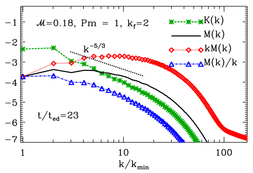
Figure 1: Power spectra of kinetic energy, $K(k)$ (green, dashed); magnetic energy, $M(k)$ (black, solid); $k\,M(k)$ (red, dotted); and $M(k)/k$ (blue, dashed-dotted) from a snapshot in the saturated state at $t/t_{\rm ed}=23$. The black dotted line shows the $k^{-5/3}$ slope for comparison. Here, the wavenumber is normalized in units of $k_{\rm min}=2\pi/L$.

In this section we present the results obtained by applying COSMIC to the data obtained from our run where the steady-state rms $\mathcal{M}\approx 0.18$. In addition to the time-series data of various physical variables, we also output three-dimensional snapshots at user-defined intervals of time in both the kinematic and saturated phases of the dynamo. These snapshots contain information about the three components of the velocity and magnetic field and the gas density on a $512^{3}$ Cartesian grid. In this work, we focus on the saturated phase of the dynamo at a time $t/t_{\rm ed}=23$, as representative of the physical conditions in this phase. For comparison, we have also used a snapshot during the kinematic stage $t/t_{\rm ed}=2$, and several additional snapshots in the saturated stage separated by least one $t_{\rm ed}$ to determine the statistical robustness of our results. For the purpose of our analysis, we choose the $x$- and $y$-axes to be in the plane of the sky and $z-$axis along the LOS. Thus, $B_{x}$ and $B_{y}$ gives rise to the polarized synchrotron emission and the magnetic field strength in the plane of the sky is $B_{\perp}=(B_{x}^{2}+B_{y}^{2})^{1/2}$. The magnetic field component parallel to the LOS is given by $B_{\|}=B_{z}$ and is thus responsible for Faraday rotation and frequency-dependent Faraday depolarization.

Before we delve into the details of the Faraday depth and the associated properties of the polarized emission, we briefly assess the characteristics of the turbulence and the dynamo-generated magnetic fields obtained from the simulation. We show in Fig. 1 the power spectra of (a) kinetic energy, $K(k)$ (green dashed with asterisks); (b) magnetic energy, $M(k)$ (black solid); (c) spectra of $k\,M(k)$ (red, dotted with diamonds), i.e. the largest energy carrying scale of the field; and (d) that of $M(k)/k$ (blue, dash-dotted with triangles) from a snapshot in the saturated phase of the dynamo. Here, $k$ is the wave number. It is evident from the plot that $M(k)$ exceeds $K(k)$ on all but the largest scales. The peak of $M(k)$ lies at $\sim 1/4-1/6$-th of the box size corresponding to physical scales of $\sim 128-85\,{\rm kpc}$, while the peak of $k\,M(k)$ occurs on scales even smaller than that of $M(k)$ (at $\sim 51\,{\rm kpc}$). On the other hand, the peak of $M(k)/k$ occurs on a scale similar to the forcing scale of $K(k)$. In the next subsection, we focus on the Faraday depth, and discuss the qualitative similarity of its spectrum to the spectrum of $M(k)/k$.

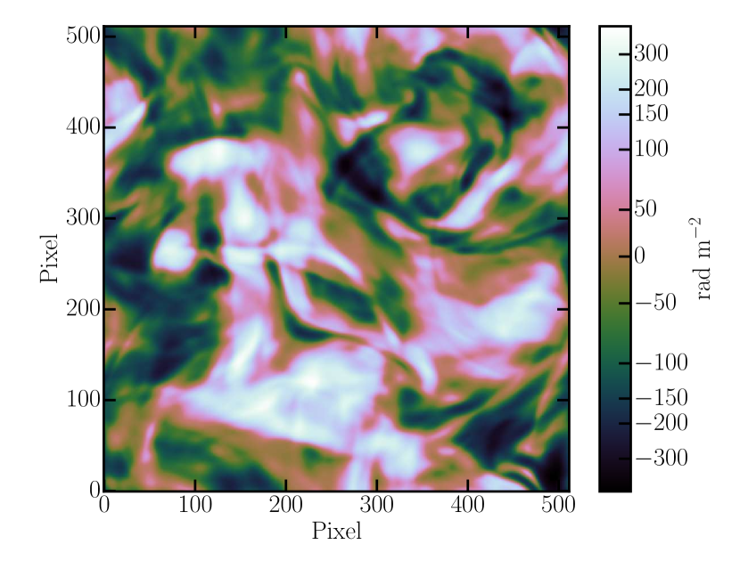
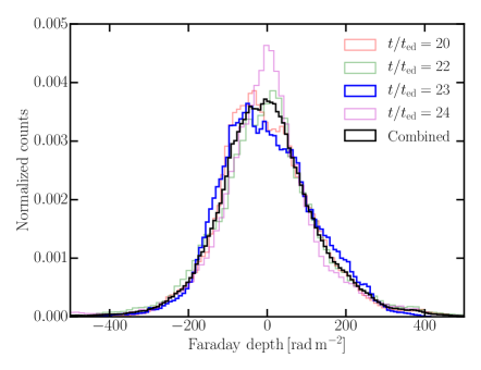
Figure 2: Top: Faraday depth map at $t/t_{\rm ed}=23$. Bottom: Distributions of Faraday depth for different snapshots in time in the saturated stage. Each snapshot is separated by at least one eddy turnover time and shows the general stability of the statistics for $t/t_{\rm ed}=23$, the highlighted blue histogram corresponding to the top panel, used for analysis in this work. The black histogram shows the combined distribution for all the runs.

4.1 Faraday depth

Much of what we know about magnetic fields in the ICM is derived from observations of the Faraday depth (FD) (Clarke et al., 2001; Vogt & Enßlin, 2003; Bonafede et al., 2010, 2015; Böhringer et al., 2016):

$${\rm FD}=K\int n_{\rm e}\,B_{\|}\,dl\,,$$ (1)

where the integration is along the LOS from the source to the observer, with $K=0.812$ rad m^-2 cm³ $\,{\rm\mu G}^{-1}$ pc^-1. Following the procedure outlined in Section 3, the mean number density of thermal electrons in the volume is $\langle n_{\rm e}\rangle=10^{-3}\,{\rm cm^{-3}}$. Because of the incompressible nature of our run, we find over densities $\delta\,n_{\rm e}/n_{\rm e}\sim\mathcal{M}^{2}\sim 3$ per cent for $\mathcal{M}\approx 0.18$, implying that $n_{\rm e}$ is roughly uniformly distributed in the simulated volume. Therefore, the Faraday depth and depolarization studied here predominantly originate from fluctuations in the magnetic field. The top panel in Fig. 2 shows the FD map in the plane of the sky obtained from a snapshot in the saturated state of the dynamo at $t/t_{\rm ed}=23$. The solid blue histogram in the bottom panel of Fig. 2 shows the corresponding PDF of FD. The detailed procedure to compute the FD maps from the simulation data is described in Appendix A and in Basu et al. (2019). We find that the value of FD lies in the range $-438$ to $+415\,{\rm rad\,m^{-2}}$ with a mean of almost zero and a dispersion, $\sigma_{\rm FD}\approx 118\,{\rm rad\,m^{-2}}$. This relatively large dispersion in FD is a consequence of fluctuations in the magnetic field component along the LOS.

In order to account for the fact that the above snapshot is not special in any way, we also computed $\sigma_{\rm FD}$ for three additional snapshots at different times in the saturated state. The PDFs of the FD from these snapshots are also shown in the bottom panel of Fig. 2. Note that each one of these snapshots corresponds to a random realization of the non-linear state of the dynamo. We find that $\sigma_{\rm FD}\approx 110\textrm{--}130\,{\rm rad\,m^{-2}}$. These values are similar to the observational estimates of $\sigma_{\rm FD}$ in the ICM determined using FD measured towards background polarized sources (Clarke et al., 2001) and Faraday depolarization measured in polarized relic embedded in a cluster medium (Kierdorf et al., 2017). Overall, the shape of the individual distributions are very similar to each other, implying that the non-linear saturated states of the dynamo at different times are statistically equivalent. Even though the individual components of the field are expected to have a non-Gaussian distribution, the FD is a sum of $B_{\|}=B_{z}$ over several independent magnetic correlation cells. The PDF of FD is also calculated over several independent areas in the $x-y$ plane, and over several independent snapshots. Consequently, the PDF of the sum is likely to tend to a Gaussian distribution. Indeed, the Gaussian nature of the PDF is clearly confirmed by the thick solid black histogram which represents the combined distribution of the four snapshots.

Earlier work by Cho & Ryu (2009) and Bhat & Subramanian (2013) has shown that the LOS integral of the magnetic field, has a variance which is related to the magnetic integral scale $L_{{\rm int},M}$. In the subsonic turbulence considered here, where $n_{\rm e}$ is roughly constant, this variance is also proportional to $\sigma_{\rm FD}$, which for a statistically homogeneous and isotropic random magnetic field is given by

$$\sigma_{\rm FD}=K\,\langle n_{\rm e}\rangle\,\frac{b_{\rm rms}}{2}\sqrt{L\,L_{{\rm int},M}}\,,\qquad L_{{\rm int},M}=\frac{2\,\pi\int(M(k)/k)\,dk}{\int M(k)\,dk}.$$ (2)

For the saturated state at $t/t_{\rm ed}=23$, we get $b_{\rm rms}\approx 1.3\,{\rm\mu G}$ and $L_{{\rm int},M}=112.4\,{\rm kpc}$. Adopting $L=512\,{\rm kpc}$ as the path length, $\langle n_{\rm e}\rangle=10^{-3}$ cm^-3, we get from equation (2) $\sigma_{\rm FD}=126.6\,{\rm rad\,m^{-2}}$, which is in good agreement with $\sigma_{\rm FD}$ determined directly from the PDF of the FD using the simulation data.

More importantly, equation (2) suggests that the FD power spectra could be qualitatively similar to the power spectra of $M(k)/k$ shown in Fig. 1. To check this, we use the 2D maps of the Faraday depth to compute the power spectra of FD at three different times – one in the kinematic phase ($t/t_{\rm ed}=2$) and at two intervals ($t/t_{\rm ed}=16.6,23$) in the saturated phase of the dynamo. The results are shown in Fig. 3. We find that the spectra remains flat on large scales in the range $k\sim 1-3$ with minor fluctuations on much smaller scales $k>8$. Due to the subsonic nature of the turbulent driving, the structures seen in the 2D map and thereby in the power spectra at any given time arises purely from the spatial fluctuations of $B_{\|}$. In order to explore how the FD power spectra compares with that of $M(k)/k$, we over plotted the spectra of $M(k)/k$ at $t/t_{\rm ed}=2,23$ by scaling it by a factor such that it overlaps with the FD power spectra at the forcing scale. In the figure these are shown by the dashed magenta and green curves, respectively.

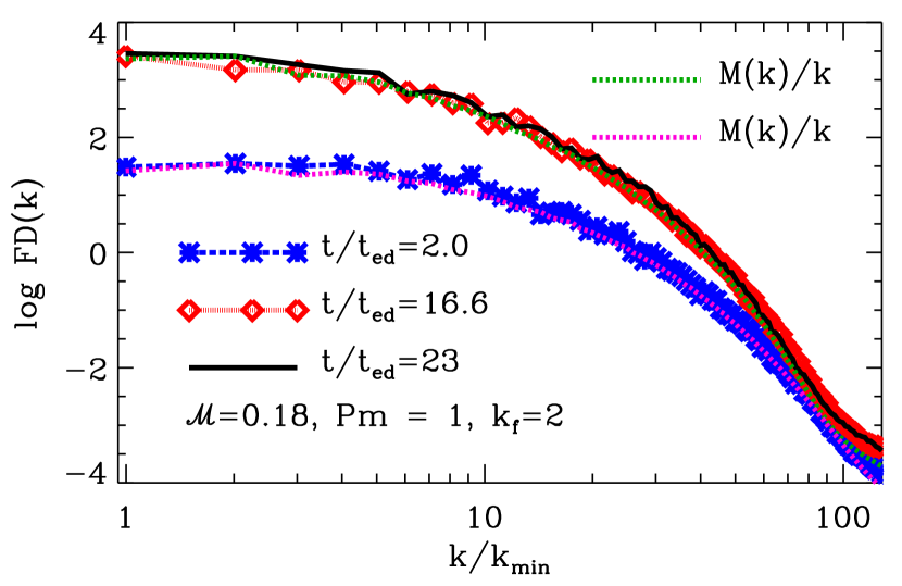
Figure 3: Power spectra of the Faraday depth. The red dotted, blue dashed, and the solid black curve correspond to the spectra in the kinematic and saturated phases, respectively. For comparison, the magenta and green dashed curves show the scaled spectra of $M(k)/k$ at $t/t_{\rm ed}=2$ and $23$, respectively. Here, the wavenumber is normalized in units of $k_{\rm min}=2\pi/L$.

Remarkably, the power spectrum of FD is strikingly similar to that of $M(k)/k$ in both the kinematic and saturated phases of the dynamo over the entire range of wave numbers shown here. Thus, the observationally determined power spectrum of FD can be used to directly infer the power spectrum of the random magnetic field in the ICM provided fluctuations in $n_{\rm e}$ are small, and values of FD are robustly estimated (see Section 6 below). The plot further shows that, compared to the kinematic phase, the FD power spectrum and that of $M(k)/k$ have more power on all but the very smallest scales in the saturated phase. This is related both to the smaller field strength and smaller integral scale during the kinematic stage of the fluctuation dynamo. Thus the power spectrum of Faraday depth in galaxy clusters contains crucial information even on the evolutionary stage of turbulent dynamo operating in them. Moreover, the top panel of Fig. 2 shows that the maximum scale of the structures seen in the 2D map of FD are comparable to the forcing scale of turbulence, and so this scale can also then be inferred from FD maps.

4.2 Total synchrotron intensity

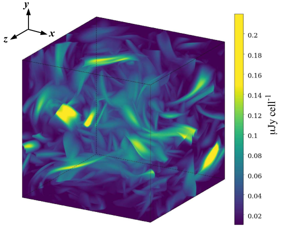
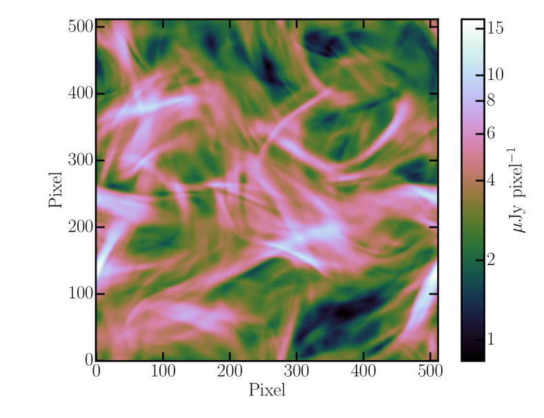
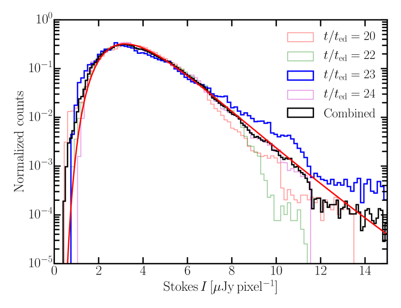
Figure 4: Top: 3D volume rendering of synchrotron emissivity at $1\,{\rm GHz}$ at $t/t_{\rm ed}=23$ in the saturated phase of the dynamo. Middle: 2D map of synchrotron intensity in the plane of the sky at $1\,{\rm GHz}$ obtained by integrating the 3D emissivity shown in the top panel along the LOS ($z$-axis). Bottom: Distributions of the total intensity for four different snapshots in the saturated stage. The solid black histogram is the combined distribution of the different snapshots and the solid red curve is the best-fitting lognormal distribution.

We calculate the total synchrotron intensity ($I_{\rm sync}$) at a frequency $\nu$ from the LOS integration of the synchrotron emissivity ($\varepsilon_{\rm sync,\nu}$) along the $z$-axis following equation (4). The top panel of Fig. 4 shows the 3D volume rendering of the synchrotron emissivity in units of $\rm{\mu Jy}\,{\rm cell}^{-1}$, while the middle panel shows the 2D map of the synchrotron intensity ($I_{\rm sync}$) integrated along the LOS at 1 GHz in the saturated state of the dynamo at $t/t_{\rm ed}=23$. In accordance with the normalization defined in Section 3, the 2D map has a total flux density of 1 Jy. Both the 3D volume rendering and the 2D map shows bright structures extending to about $1/2$ the scale of the box that corresponds to the size of the turbulent cells. Since we have assumed a constant distribution of $n_{\rm CRE}$, $\varepsilon_{\rm sync}\propto B_{\perp}^{1-\alpha}$, and the total intensity $I_{\rm sync}\propto\int\,B_{\perp}^{2}\,dl$ (for $\alpha=-1$), the structures seen here essentially arises due to the magnetic fields, which are being randomly stretched and twisted due to turbulent driving.

In the bottom panel of Fig. 4, we show the PDF of $I_{\rm sync}$ at four different times during the saturated phase. It is clear from the plots that, unlike the distribution of FD, the histograms of each of these are well represented by lognormal distribution, and the best fit to the combined black distribution is shown by the solid red curve in the figure. Since the total synchrotron intensity in spatially resolved objects depends non-linearly on the magnetic field, the distribution is not expected to be a Gaussian. It is interesting to note that, when the small-scale features are resolved in the synthetic total intensity maps obtained at the native resolution of the simulations, the lognormal distribution has long tails. However, the extent of the tail towards higher flux values goes down drastically, making the distributions more symmetric when synthetic observations are smoothed to mimic observations performed using a telescope. This is perhaps the reason why small-scale structures seen in the $I_{\rm sync}$ map in Fig. 4 (middle panel) have not yet been observed in astronomical observations of ICM. Smoothing of the observable quantities introduced by a telescope has strong implications on polarization and we discuss that in detail in Section 5.

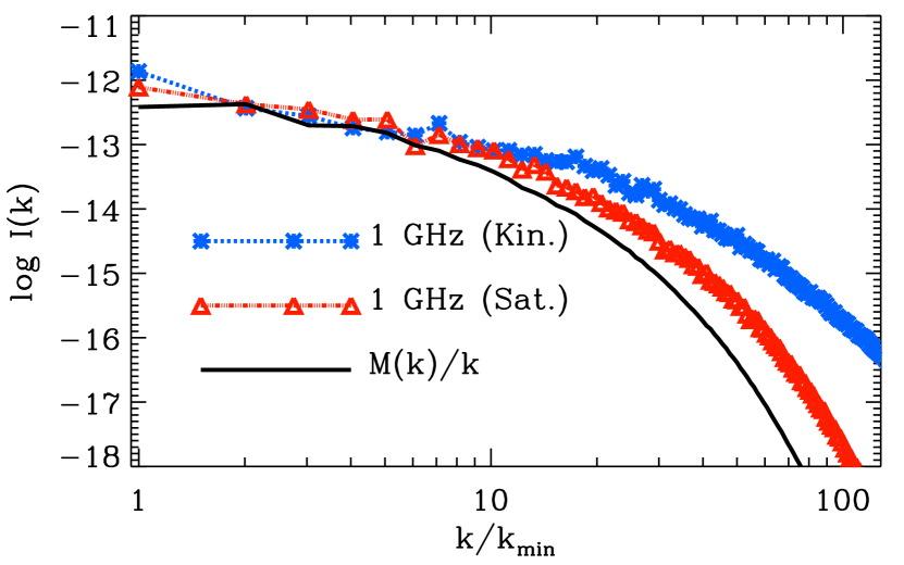
Figure 5: Power spectra of the total synchrotron emission ($I$) at $1\,{\rm GHz}$ in the kinematic (blue, dotted line with asterisks) and in the saturated phase (red, dashed line with open triangles). The solid black line shows the scaled spectra of $M(k)/k$. The wavenumber is normalized in units of $k_{\rm min}=2\pi/L$.

0.5 GHz	1 GHz	6 GHz
	Polarized intensity
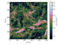
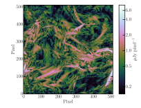
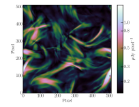
	Fractional polarization
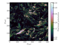
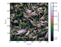
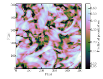
	Polarized intensity (smoothed 10 pixels)
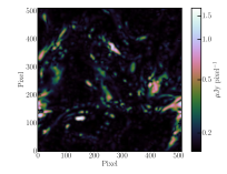
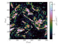
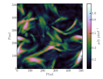
	Fractional polarization (smoothed 10 pixels)

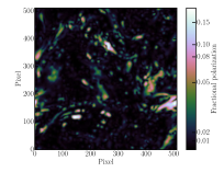
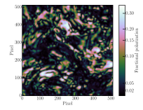
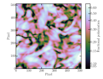
Figure 6: First row: Polarized intensity maps in units of Jy pixel^-2. Second row: Fractional polarization maps. The third and fourth rows show the quantities after smoothing by a Gaussian kernel with FWHM 10 pixels. The left-hand, middle, and right-hand columns are at 0.5, 1 and 6 GHz, respectively, at $t/t_{\rm ed}=23$.

In Fig. 5, we show the power spectra of the total intensity at $1\,{\rm GHz}$. The spectrum at $t/t_{\rm ed}=2$ in the kinematic phase is shown in blue dashed line with asterisks while that at $t/t_{\rm ed}=23$ in the saturated phase is shown by the red dotted curve with open triangles. Both the curves show that the amplitude at wave numbers $k\leq 10$ is independent of the evolutionary stage of the dynamo and is peaked on the scale of the simulation domain (i.e. at $512\,{\rm kpc}$). However, the spectrum in the saturated state falls off with a steeper slope on scales $k>10$, compared to the kinematic phase suggesting the presence of more structures on these scales, similar to what was seen for FD power spectra. The spectra at two other representative frequencies corresponding to $0.5$ and $6\,{\rm GHz}$ (not shown in the figure) also show similar behavior. Since the total intensity $I\propto\nu^{-\alpha}$, the amplitude of the spectra decreases as the frequency increases from $0.5-6\,{\rm GHz}$. We also find that the overall shape of the scaled spectrum of $M(k)/k$ in the saturated state resembles that of the red curve to a fair degree in the range $2\leq k\leq 6$, corresponding to physical scales $256\,{\rm kpc}\geq l\geq 85\,{\rm kpc}$.

4.3 Polarization parameters

In this subsection, we focus on extracting the polarization parameters from the simulation data and exploring how these parameters depend on the frequency. To this end, we computed the frequency dependence of the linearly polarized intensity (${\rm PI}_{\nu}$) from the Stokes $Q$ and $U$ using equations (7)–(9) and the fractional polarization $p_{\nu}={\rm PI}_{\rm\nu}/I_{\rm sync,\nu}$ from a single snapshot of the magnetic field in the saturated state.

In Fig. 6, the first two rows show the 2D maps of the total polarized intensity (first row) and the fractional polarization (second row) at three different frequencies: $0.5\,{\rm GHz}$ (first column), $1\,{\rm GHz}$ (second column), and $6\,{\rm GHz}$ (third column). The corresponding Stokes $Q$ and $U$ parameters are presented in the top two panels of Fig. 12 in the Appendix. Basic pixel-wise statistics of the polarization parameters at these three representative frequencies are presented in Table 3, in surface brightness units of Jy pixel^-1. Note that this is equivalent to performing observations with a sufficiently small telescope resolution that is same as that of the pixel size of these MHD simulations.

The pixel-wise mean and maximum polarized intensities shown in the first row of Fig. 6 progressively decrease from $0.5$ to $6\,{\rm GHz}$ (see Table 3). This trend arises due to a mix of frequency-dependent Faraday depolarization and the spectral dependence of total synchrotron emission. The PDF of polarized intensity at 6 GHz is found to be similar to lognormal distribution as seen for total intensity. However, at lower frequencies, due to structures introduced by Faraday depolarization, the PDFs show extended power-law tails. Spectral effects of Faraday depolarization are seen in the frequency variation of the fractional polarization, the maps of which are shown in the second row of Fig. 6. In contrast to ${\rm PI}_{\nu}$, these maps show the opposite trend with mean $p$ increasing significantly from $\langle p\rangle=0.09$ at $0.5\,{\rm GHz}$ to $\langle p\rangle=0.345$ at $6\,{\rm GHz}$. Note that, although the strengths of magnetic field components are random and there are no mean fields in the simulated turbulent media (due to the non-helical nature of turbulence and lack of scale separation), the mean fractional polarization at $6\,{\rm GHz}$ is relatively high where the frequency-dependent Faraday depolarization is low. This is because, fields that are stretched and twisted by dynamo action can be ordered locally on the scale of turbulent driving. Moreover, due to relatively low number of magnetic field integral scales (of the order of five) in the simulation volume used here, the cancellation of the polarized emission along the path-length is low and, along with locally ordered fields, partially contributes towards the high fractional polarization. At low frequencies, depolarization due to Faraday rotation along the LOS play a significant role in reducing the observed fractional polarization.

For a longer path-length $L$ these predictions are likely to decrease as $L^{-1/2}$. Therefore, for a longer path-length of, say, a few Mpc, the decrease in polarization would be a factor of the order of two. However, magnetic field strength, $n_{\rm CRE}$, and $n_{\rm e}$ in galaxy clusters are all likely stratified, decreasing away from cluster core over scales of order a few hundred kpc, their core radii. So, the relative contribution to total and polarized intensities from longer path-lengths will also decrease along the LOS as one moves away from the cluster core, and the cancellation of polarization due to random fields and Faraday depolarization will be dominated by the domain with largest magnetic field strengths, cosmic ray and free electron densities. In this case, the estimated polarization using a box scale of 512 kpc, is expected to be reasonable up to factors of the order of two.

Table 3: Summary of statistics of Stokes ${\rm PI},Q,U$ and the fractional polarization ($p$) at native-pixel and 10-pixel FWHM resolutions.

Quantity	Resolution	Mean				Median				Dispersion
		0.5 GHz	1 GHz	6 GHz		0.5 GHz	1 GHz	6 GHz		0.5 GHz	1 GHz	6 GHz
Stokes $PI$	Native	0.670	0.638	0.228		0.521	0.519	0.192		0.571	0.496	0.163
($\rm\mu Jy\,pixel^{-1}$)	10 pixels	0.099	0.227	0.222		0.053	0.156	0.190		0.130	0.218	0.151
Stokes $Q$	Native	0.005	0.007	-0.038		0.002	0.000	-0.030		0.625	0.572	0.180
($\rm\mu Jy\,pixel^{-1}$)	10 pixels	0.005	0.007	-0.038		0.001	0.001	-0.031		0.120	0.224	0.171
Stokes $U$	Native	0.000	-0.003	-0.035		0.003	-0.006	-0.027		0.620	0.570	0.209
($\rm\mu Jy\,pixel^{-1}$)	10 pixels	0.000	-0.003	-0.035		0.001	-0.004	-0.026		0.111	0.221	0.200
$p$	Native	0.090	0.169	0.345		0.077	0.155	0.346		0.061	0.094	0.129
	10 pixels	0.013	0.060	0.337		0.008	0.044	0.336		0.015	0.052	0.126

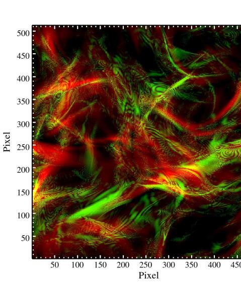
Figure 7: Overlay of the total synchrotron intensity (in red) and the polarized intensity at $0.5\,{\rm GHz}$ (in green). Both the maps are saturated towards lower surface brightness to show the close correspondence between bright filamentary structures observed in polarization with that of total intensity (see text in Section 4.3).

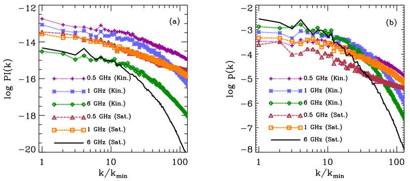
Figure 8: Power spectra of the total polarized intensity (left) and the fractional polarization (right) at 0.5, 1, and 6 GHz in the kinematic ($t/t_{\rm ed}=2$) and saturated phase ($t/t_{\rm ed}=23$). The wavenumber is normalized in units of $k_{\rm min}=2\pi/L$.

In our simulated volume, of particular importance is the fact that strong frequency-dependent Faraday depolarization at lower frequencies ($\lesssim 1.5\,{\rm GHz}$) gives rise to small-scale structures on scales much smaller than the driving scale of turbulence. These small-scale structures appear sharper at lower frequencies (near $\sim 0.5\,{\rm GHz}$) resembling filament-like features similar to the polarization filaments observed in the Galactic interstellar medium (Shukurov & Berkhuijsen, 2003; Fletcher & Shukurov, 2006; Zaroubi et al., 2015; Jelić et al., 2015; Jelić et al., 2018). Although these features are not readily visible in the total synchrotron intensity emission (Fig. 4 middle panel) or in the Faraday depth (Fig. 2) maps, with a cursory look, they somewhat correspond to sharp edges observed in the total synchrotron intensity (see Fig. 7).

In the left- and right-hand panels of Fig. 8, we present the power spectra of the ${\rm PI}_{\nu}$ and $p_{\nu}$, respectively. The effects of the small-scale structures introduced due to Faraday depolarization towards low frequencies are easily discernible as larger power at large $k$ in the power spectra of the polarized intensities shown in Fig. 8 and the Stokes $Q$ and $U$ parameters shown in Fig. 10. At higher frequencies, the power spectra of the polarization parameters appear similar to that obtained for the total synchrotron intensity and the Faraday depth map. A direct comparison of the power spectra of ${\rm PI}_{\nu}$ with that of the Stokes $Q$ and $U$ (see Appendix B) reveals that at low frequencies near $0.5\,{\rm GHz}$ the power spectra of $Q$ and $U$ parameters remain flat over the entire range of $k$, while in contrast the spectrum of ${\rm PI}_{\nu}$ falls off at large $k$. This is because strong Faraday rotation and depolarization give rise to strong fluctuations in the values of Stokes $Q$ and $U$ parameters that are changing signs on scales of pixel resolution of these MHD simulations.

An interesting feature is noticed in the power spectra of Stokes $Q$ and $U$ parameters. In the saturated phase, due to stronger magnetic field strengths, Faraday rotation effects at low frequencies (around $0.5\,{\rm GHz}$) significantly wipe out any resemblance to the power spectra of ${\rm PI}$ and FD on all scales. This is, however, not the case during the kinematic stage and correlated structures in Stokes $Q$ and $U$ are observed on scales of few tens of pixels. Such a trend, if seen in astronomical observations, could allow us to identify the evolutionary stage of a fluctuation dynamo operating in galaxy clusters.

4.3.1 Correlation scales

Table 4: Values of the integral scales (in kpc) of the velocity ($L_{{\rm int},V}$), magnetic fields ($L_{{\rm int},M}$), Faraday depth ($L_{\rm int,FD}$), the total synchrotron intensity ($L_{{\rm int},I}$) at $1\,{\rm GHz}$, and the polarized intensity ($L_{{\rm int},{PI}}$) at $0.5,1$ and $6\,{\rm GHz}$ at two different times in the steady state.

$t/t_{\rm ed}$	$L_{{\rm int},V}$	$L_{{\rm int},M}$	$L_{\rm int,FD}$	$L_{{\rm int},I}$	$L_{{\rm int},PI}~{}(\,{\rm kpc})$
	$(\,{\rm kpc})$	$(\,{\rm kpc})$	$(\,{\rm kpc})$	$(\,{\rm kpc})$	$0.5\,{\rm GHz}$	$1\,{\rm GHz}$	$6\,{\rm GHz}$
16.6	320	106	212.5	224	122	155	199
23	340	112.4	216	227.6	138	128	182

It is often of interest to relate the correlation scales or the integral scales of observable quantities like the total and polarized intensity of the synchrotron emission to those corresponding to the random magnetic and velocity fields. We can measure these directly from our simulation, using the power spectra discussed above. We define these from the 1D spectra of various quantities, as for the magnetic integral scale $L_{{\rm int},M}$ defined in equation (2). Table 4 shows the values of these integral scales (in $\,{\rm kpc}$) computed from two different snapshots in the saturated phase of the dynamo corresponding to $t/t_{\rm ed}=16.6$ and $23$. This allows us to check the sensitivity of these scales to random fluctuations in the field. In both cases, we find that the velocity integral scale, $L_{{\rm int},V}\sim 3\,L_{{\rm int},M}$. It is further evident that, although there is some random scatter from one realization to another, the integral scales associated with all the observables, FD, $I_{\rm sync}$ and the high-frequency ${\rm PI}$ are all comparable and larger than the magnetic integral scale by a factor of about two (Table 4). However, for the polarized intensity these are frequency dependent due to the effect of Faraday depolarization. The integral scales at lower frequencies are generally smaller, due to small-scale structures introduced by Faraday depolarization.

5 Smoothed polarization parameters

So far we have presented results from synthetic broad-band observations obtained at the native-pixel resolution of the simulations. In order to make any meaningful connection between the synthetic observations and astronomical observations performed using a radio telescope with finite resolution, it is necessary to smooth the synthetic maps. A finite telescope resolution, referred to as the beam, has a significant impact on the nature of structures that are observed in the plane of the sky, especially in the case when the corresponding spatial resolution is significantly larger than the intrinsic scale of emission. For positive definite quantities, such as the total intensity, the telescope beam smoothes out fine-scale structures while generally preserving larger-scale features. This, however, is not the case for polarized intensity because smoothing of the Stokes $Q$ and $U$ parameters that frequently change sign spatially leads to two types of depolarization phenomena, namely, beam and Faraday depolarization.

Beam depolarization is caused by turbulent magnetic fields on scales smaller than the beam, and is independent of the frequency of observations. In contrast, Faraday depolarization is strongly dependent on the frequency of observations, and is caused by local fluctuations in FD along the LOS as well as in the plane of the sky when linearly polarized signal propagates through magneto-ionic media (see e.g. Burn, 1966; Tribble, 1991; Sokoloff et al., 1998). This means that rapid spatial variations of Stokes $Q$ and $U$ parameters when smoothed can result in recovering polarized structures that are significantly different compared to the intrinsic structures. Stronger Faraday rotation towards frequencies below $\sim 1.5\,{\rm GHz}$ also means that the observed polarized emission can appear significantly different at different frequencies. Hence, it is crucial to investigate the effects of beam smoothing in combination with Faraday depolarization to determine optimum frequency of observations so as to gain maximum insight into the magnetic field properties of galaxy clusters with future observations.

Here we investigate the effects of smoothing by convolving the synthetic images obtained at native resolution of simulated data with a 2D Gaussian kernel. Details of the convolution process performed in COSMIC is given in Appendix A.2. In the bottom two rows of Fig. 6, we show the smoothed maps of ${\rm PI}_{\nu}$ and $p_{\nu}$. Smoothing was performed using a symmetric kernel size with full width at half-maximum (FWHM) of $10\times 10$ pixel² corresponding to Gaussian spatial smoothing on $4.25\,{\rm kpc}$ scale. We note that, at the distance of the Coma cluster of about 100 Mpc, a physical scale of 1 kpc corresponds to an angular scale of 2 arcsec, and thus this smoothing would be over a beam with FWHM of 20 arcsec. The corresponding 2D maps of the Stokes $Q$ and $U$ are shown in bottom two rows of Fig. 12.

In Fig. 6, comparing the smoothed maps with the maps at native resolution, noticeable differences in the appearance of polarization features are seen, especially at 0.5 and 1 GHz due to substantial Faraday rotation and depolarization-induced spatial fluctuations in Stokes $Q$ and $U$ parameters (see Fig. 12). It should be noted that we have saturated the colour scales of polarized intensity and fractional polarization in Fig. 6 towards lower values, roughly corresponding to typical sensitivities achievable with current radio telescopes. Fractional polarization maps are saturated below 0.02. Most of the bright filamentary structures and diffuse polarized emission that are seen at native resolution are lost in the smoothed maps at lower frequencies. Bright polarized emission at frequencies below $\sim 1.5\,{\rm GHz}$ are confined as clumpy structures that cannot be readily identified with features in either the total synchrotron intensity nor in the Faraday depth maps. These clumps are locally polarized at a level of up to $\sim 0.2$ at $0.5\,{\rm GHz}$, and, up to $\sim 0.4$ level at 1 GHz. However, with increasing frequency, the regions with large values of $p$ become more volume filling. At a higher frequency of $6\,{\rm GHz}$, where the effects of Faraday rotation are low, both the native resolution and smoothed maps show similar polarized structures. This brings to light an important aspect; in the ICM where Faraday rotation and synchrotron emission are mixed, higher frequency ($\gtrsim 5\,{\rm GHz}$) observations are better suited to infer magnetic properties from observations of polarized synchrotron emission.

The effects of beam smoothing in the presence of Faraday depolarization on the statistical properties of polarized quantities at different frequencies can be seen quantitatively in Table 3. The magnitude to which a telescope beam affects polarization is best studied in the context of fractional polarization because the values of other polarization parameters depend on the spectral variation due to both Faraday depolarization and the overall synchrotron spectrum. This can be seen in the statistical values of ${\rm PI}_{\nu}$ of the smoothed maps (in Table 3), which, unlike the maps at native resolution, has comparatively higher values at $1\,{\rm GHz}$ with respect to those at $0.5$ and $6\,{\rm GHz}$. Also note that the mean and median values of Stokes $Q$ and $U$ parameters do not change significantly after smoothing across frequencies and remain close to zero. This is because, in the absence of a mean magnetic field in the simulated volume, their values are intrinsically distributed around zero mean. However, a telescope beam smooths out large spatial fluctuations in the values of the Stokes parameters, which manifests as reduced dispersion, except at a higher frequency of $6\,{\rm GHz}$ where Faraday rotation affects polarized structures the least (see Table 3). This again points to the fact that observations at frequencies above $\sim 5\,{\rm GHz}$ better represent the intrinsic statistical properties of polarized emission from ICM.

Smoothing introduced by a telescope beam has a drastic effect on the observable fractional polarization from the diffuse ICM. Although the median fractional polarization from the diffuse ICM obtained at native resolution decreases substantially with decreasing frequency from $p_{\rm 6\,GHz}\approx 0.35$ to $p_{\rm 0.5\,GHz}\lesssim 0.1$ (see Table 3), they are still at a level such that polarization from fainter diffuse regions could be measured. However, the smoothed maps at lower frequencies have significantly lower fractional polarization with median $p_{\rm 0.5\,GHz}\lesssim 0.01$ and $p_{\rm 1\,GHz}\lesssim 0.1$. In fact, smoothing increases the relative fluctuations of $p$ with respect to its mean at lower frequencies, i.e. at $0.5\,{\rm GHz}$, $\sigma_{p}/\langle p\rangle$ increases from $\sim 0.7$ at the native resolution to $\sim 2$ after smoothing. Similar to other polarized quantities, the statistical properties of fractional polarization at $6\,{\rm GHz}$ are not significantly affected by beam smoothing.

To assess the severity of the beam smoothing, we further performed smoothing with kernels having FWHM of $30\times 30$ and $50\times 50$ pixel². These represent Gaussian smoothing on linear scales of $12.75$ and $21.23\,{\rm kpc}$, respectively. Keeping the angular resolution of $10\times 10$ arcsec² (FWHM) the same, these smoothing scales correspond to galaxy clusters roughly at redshifts $0.06$ and $0.12$ using cosmological parameters from Planck 2018 results (Planck Collaboration et al., 2020). We find that smoothing on larger physical scales of $\sim 20$ kpc decreases $\langle p\rangle$ at lower frequencies by factors of 10–20 as compared to native resolution, with values significantly lower than 0.01 at $0.5\,{\rm GHz}$; at $1\,{\rm GHz}$, $\langle p\rangle$ is expected only at a level of $\sim 0.02$. In such cases, the clumpy polarized structures fill much less sky area as compared to smoothing by $10\times 10$ pixel² discussed above. Larger smoothing scales, however, affects the polarization properties at $6\,{\rm GHz}$ less severely as compared to those at 0.5 and $1\,{\rm GHz}$ with $p$ decreasing by up to $\sim 20$–25  per cent on smoothing by $50\times 50$ pixel². Therefore, for distant galaxy clusters, our study suggests high-frequency observations can circumvent beam smoothing issues. In addition, to minimize spatial correlation within the beam for power spectra analyses, high angular resolution $\lesssim 1\times 1$ arcsec² is required, which will also help to infer intrinsic spatial structures of polarized emission.

6 Application of RM synthesis

Magnetic fields in the ICM have been inferred via FD measured towards polarized sources located behind galaxy clusters. Alternatively, they could also be probed if the galaxy cluster itself has polarized synchrotron emission. Here we assume this to be the case to compute FD and fractional polarization from synthetic broad-bandwidth observations of this emission by applying the commonly used techniques of RM synthesis (Brentjens & de Bruyn, 2005) and RM CLEAN (Heald et al., 2009).

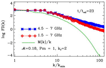
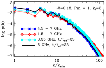
Figure 9: Power spectra of the $\rm FD_{RM\,synth}$ (left) and the fractional polarization (right) maps obtained by applying RM synthesis to synthetic spectro-polarimetric observations in the frequency range $1.5\textrm{--}7\,{\rm GHz}$ (red points) and $4.5\textrm{--}7\,{\rm GHz}$ (blue points). The power spectrum of $M(k)/k$ is shown in green (same as Fig. 3), and the power spectra of the fractional polarization at $3.25$ and $6\,{\rm GHz}$ obtained directly from the synthetic maps are shown as the light-blue points and black curve, respectively (see text for details). The wavenumber is normalized in units of $k_{\rm min}=2\pi/L$.

As seen in Section 4.3, Faraday depolarization affects the spatial structure of ${\rm PI}_{\nu}$ and $p_{\nu}$ at frequencies below $1.5\,{\rm GHz}$. Therefore, we explore RM synthesis and RM CLEAN applied to broad-bandwidth synthetic observations for two representative frequency coverages, between 1.5 and 7 GHz and between 4.5 and 7 GHz. For these two frequency ranges, the sensitivities to maximum observable |FD| and extended FD structures are similar, $\sim 6\times 10^{5}$ and $\sim 1700\,{\rm rad\,m^{-2}}$, respectively. However, the FWHM of the rotation measure spread function (RMSF), which determines the resolution in FD space, differs by one order of magnitude, having values of $91$ and $1330\,{\rm rad\,m^{-2}}$ for the $1.5$–$7\,{\rm GHz}$ and $4.5$–$7\,{\rm GHz}$ ranges, respectively.

We have used fractional Stokes parameters, $Q/I_{\rm sync}$ and $U/I_{\rm sync}$, for performing RM synthesis, which provides the so-called Faraday depth spectrum — fractional polarization as a function of FD, for each spatial pixel. Maps of Faraday depth ($\rm FD_{\rm RM\,synth}$) and fractional polarization ($p_{\rm RM\,synth}$) were computed from the RM CLEANed Faraday depth spectrum at each pixel. We refer the reader to Appendix C for details and only present the results here. In the left-hand panel of Fig. 9 we show the power spectra of $\rm FD_{RM\,synth}$ derived from its 2D map and, in the right-hand panel, the corresponding power spectra of $p_{\rm RM\,synth}$. These have been obtained for the two frequency ranges mentioned above. Since RM synthesis provides fractional polarization parameters at frequencies corresponding to the mean wavelength ($\lambda$)-squared of the frequency coverage (Brentjens & de Bruyn, 2005), we also show for comparison the power spectra of $p$ at $3.25$ and $5.6\,{\rm GHz}$ computed directly as in Section 4.3.

Unlike the FD power spectra shown in Fig. 3, the power spectra of the recovered $\rm FD_{RM\,synth}$ maps for both the frequency coverages deviate significantly in shape from $M(k)/k$ (the green curve in the left-hand panel of Fig. 9). This is due to a combination of poor resolution in FD space and limitations while interpreting Faraday depth spectra, which introduces spurious structures in maps of $\rm FD_{RM\,synth}$. These limitations arise due to complicated Faraday depth spectra in the presence of intermittent magnetic fields, with multiple peaks at FDs where the cumulative polarized emission binned in FD is high (see Basu et al., 2019, for details). Therefore, $\rm FD_{RM\,synth}$ at the location of the highest peak in Faraday depth spectrum may not correspond to the FD along the entire LOS of the synchrotron-emitting volume. Irrespective of the frequency coverage and/or observational noise, this underscores the limitation of extracting $\rm FD_{RM\,synth}$ and calls for sophisticated techniques of determining the FD of an LOS from Faraday depth spectra obtained for media that are both synchrotron emitting and Faraday rotating. Until such techniques are available, FD in galaxy clusters can be probed by measuring the FD of background sources that have stronger polarized emission than the cluster itself, provided one can adequately disentangle the FD structure of the background sources themselves from that of the ICM, and adequately account for discrete sampling of LOS probed by these sources.

In contrast, there is an excellent match of the power spectra of $p_{\rm RM\,synth}$ with the corresponding power spectra of $p$ for both the frequency ranges. This is because, at the effective frequencies of $3.25$ and $5.6\,{\rm GHz}$ of $p_{\rm RM\,synth}$ obtained from RM synthesis, Faraday depolarization is rather low. Moreover, as the Faraday depth spectra for these two frequency coverages remains mostly unresolved, their peaks correspond well to the expected polarization fraction. This further emphasizes the requirement for studying polarization from the ICM of galaxy clusters at high frequencies in order to extract meaningful information on their magnetic field properties.

7 Conclusions

Statistical studies of Faraday RM in a number of galaxy clusters reveal that the ICM is magnetized with $\,{\rm\mu G}$-level magnetic fields. As argued in Section 1, fluctuation dynamos are now acknowledged to be the main driver of amplification and maintenance of magnetic fields in these systems. In this paper we have explored in detail the properties of polarized emission, particularly the synchrotron emissivity and the polarization signals that arises from such turbulent dynamo action. Even though, a great deal of work has been done on Faraday RM on both the observational and theoretical fronts (Clarke et al., 2001; Carilli & Taylor, 2002; Vogt & Enßlin, 2003; Subramanian et al., 2006; Cho & Ryu, 2009; Bonafede et al., 2010; Bhat & Subramanian, 2013; Böhringer et al., 2016; Marinacci et al., 2018; Sur et al., 2018; Vazza et al., 2018; On et al., 2019), little attention has been paid to understanding the emissivity and polarization signals generated by the intermittent magnetic field structures produced by fluctuation dynamos. This is primarily because detection of polarized signals from radio halos has so far proved to be an arduous task with current radio interferometers (Vacca et al., 2010). More recent works (Govoni et al., 2013; Govoni et al., 2015; Loi et al., 2019) explore the possibility of their detection with upcoming radio interferometers like the SKA and its precursors. The issue is non-trivial to say the least as the observables themselves such as the synchrotron intensity ($I_{\rm sync}$) and the Stokes $Q$ and $U$ parameters are related to the components of the field in a non-linear manner. This in turn makes them sensitive to the underlying structures of the magnetic field.

The approach that we have adopted here is to use data from a numerical simulation of fluctuation dynamos as an input to the COSMIC package of Basu et al. (2019) to perform synthetic observations between $0.5$ and $7\,{\rm GHz}$ in the non-linear saturated state of the dynamo. Apart from the 2D and 3D maps of FD and $I_{\rm sync}$ and their associated power spectra, we paid particular attention to the frequency dependence of the Stokes $Q$ and $U$ parameters and the effects of both Faraday depolarization and beam smoothing. We further computed the power spectra of FD and $p$ by applying the technique of RM synthesis to the simulation data. We have not added any complications introduced due to observation systematics or noise. In what follows, we summarize and discuss the main findings of our work.

1. By shooting LOS through the simulation volume we obtained $\sigma_{\rm FD}\sim 100\,{\rm rad\,m^{-2}}$ across four statistically independent realizations of the non-linear saturated state of the dynamo. These values are in close agreement with the observed values in the ICM. The PDF of FD (in the non-linear steady state) is well represented by a Gaussian distribution in each of the snapshots (see Section 4.1). While previous theoretical studies had hinted at a possible relation between the LOS integral of the magnetic field and the magnetic integral scale, here we confirm for the first time that the power spectrum of FD is strikingly similar to that of $M(k)/k$ over the entire range of scales. This implies that one can in principle reconstruct the power spectrum of the random magnetic fields by observationally determining the FD power spectrum, at least in bulk of the ICM where turbulence is believed to be subsonic. Moreover, in the ICM where turbulence is driven by a combination of mass accretion from filaments and major and minor mergers, the scale of structures in FD can be correlated at the most on the scale of turbulent driving.

2. Analysis of the total synchrotron emission reveals that both 3D volume rendering and the 2D map also show bright structures extending to about half the scale of the box. Because of the assumed constant distribution of cosmic ray electrons, these structures essentially represent the effects of random stretching and twisting of the field lines due to random turbulent driving. However, unlike the Gaussian PDF obtained for the FD, we find that the PDFs of total synchrotron intensity show a distinct lognormal distribution.

3. In accordance with the stated objectives of this work we probed in detail the frequency dependence and effects of finite size of the telescope beam on the polarization parameters (${\rm PI}_{\nu}$, $p_{\nu}$, Stokes $Q$ and $U$) at three representative frequencies, $0.5,1$ and $6\,{\rm GHz}$. Our key observations are as follows :

   1. Frequency-dependent Faraday depolarization significantly affects polarized structures observed at low radio frequencies ($\lesssim 1.5\,{\rm GHz}$). This leads to the emergence of small-scale structures on scales much smaller than the driving scale of turbulence (see e.g. the top row in Fig. 6). The presence of these small-scale structures is further confirmed by larger power at large $k$ in the power spectra of ${\rm PI}_{\nu}$ shown in Fig. 8. Concomitantly, fractional polarization is relatively high where frequency-dependent Faraday depolarization is low and vice versa.

   2. Map of ${\rm PI}$ at low frequencies of $0.5\,{\rm GHz}$ shows strong spatial variations on small scales. This results in flattening of the power spectra of Stokes $Q$ and $U$ on all scales as seen in Fig. 10. This poses a serious challenge while inferring magnetic field properties from low frequency observations.

   3. Careful analysis of the power spectra of Stokes $Q$ and $U$ reveal that, in contrast to the kinematic stage, Faraday rotation effects at $0.5\,{\rm GHz}$ erase any resemblance to the power spectra of ${\rm PI}_{\nu}$ and FD on all scales. This provides an opportunity to diagnose the evolutionary stage of the dynamo in astronomical observations.

   4. Comparison of the smoothed maps of ${\rm PI}_{\nu}$ and $p_{\nu}$ with those at the native-pixel resolution of the simulations reveals that higher-frequency observations ($\gtrsim 5\,{\rm GHz}$) should be ideally preferred as they better represents the statistical properties of the polarized emission of the ICM and are therefore more suited to infer magnetic field structures in the ICM.

4. The power spectra of FD obtained from RM synthesis applied to polarized emission in frequency bands $4.5\textrm{--}7\,{\rm GHz}$ and $1.5\textrm{--}7\,{\rm GHz}$ deviate significantly in shape from the power spectrum $M(k)/k$. On the other hand, the power spectra of $p$ obtained using the same technique match accurately those computed directly from the simulated data for both frequency ranges.

8 Discussion and Outlook

Our key findings outline the importance of and need for high-frequency observations in order to gain an understanding of the properties of polarized emission together with the structural properties of random magnetic fields in the ICM. In this regard, Band 5 of SKA ($4.6\textrm{--}15.3\,{\rm GHz}$) will be ideally suited to detect polarized emission from the ICM. Our work clearly demonstrates that at frequencies below $1\,{\rm GHz}$ a combination of low sensitivity and observation noise, will result in polarized emission to be detected only from bright filamentary structures that could originate either due to shock compression or from Faraday depolarization. Thus, such detections may not provide adequate information on the global properties of turbulent magnetic fields in the ICM.

We find that the telescope beam drastically affects the properties of polarized emission in the presence of Faraday rotation at low frequencies. At frequencies below $\sim 1\,{\rm GHz}$, depolarization within the beam is dominated by fluctuations introduced by Faraday rotation and the polarized structures are confined as clumps. For radio-frequency observations of ICM performed at frequencies near $0.5\,{\rm GHz}$ with an angular resolution of $10\times 10$ arcsec² sampled with 1 arcsec pixels, our synthetic maps suggests that these clumps have median fractional polarization at the level of a few per cent, reaching a maximum of $\sim 20$ per cent with a polarized intensity of $\sim 20\,\rm{\mu Jy}$ beam^-1. This means that, in order to detect polarization at more than $5\sigma$ (to reduce Ricean bias; Wardle & Kronberg, 1974), a sensitivity of $\sim 4\,\rm{\mu Jy}$ beam^-1 is needed. Detecting such levels of polarized emission will be a challenging proposition with telescopes currently operating at these frequencies or with the SKA-LOW, and, if detected at all, they are expected to be highly sporadic in nature, and even more so in the presence of realistic noise. This will hamper the inference of any meaningful information on the turbulence properties of ICM magnetic fields through observations performed at frequencies below $1\,{\rm GHz}$. We find that detecting polarized emission from ICM below $1\,{\rm GHz}$ and inferring the magnetic field properties are already difficult in the absence of realistic observations noise. We will address additional complications introduced by noise in a follow-up study. We emphasize that the flux densities and the sensitivity presented in this work are normalized for a Coma-like nearby cluster. Therefore, our assumed total synchrotron flux density of 1 Jy at 1 GHz, and thereby the estimated sensitivity requirements above, are already significantly higher than that expected for distant galaxy clusters.

In contrast, the telescope beam does not significantly affect the polarized emission at frequencies above $5\,{\rm GHz}$; and, the median level of polarization increases to about 30 per cent (see Table 3) and the diffuse polarized intensity is expected to be few tens of $\rm{\mu Jy}$ beam^-1. ICM observations with the Karl G. Jansky Very Large Array (VLA) in the $4\textrm{--}8\,{\rm GHz}$ frequency range can detect such levels of polarized intensity with rms noise of few $\rm{\mu Jy}$ beam^-1. However, a challenge is faced with the fact that the Stokes $Q$ and $U$ parameters maps could have diffuse large-scale structures that span up to about $200\,{\rm kpc}$. This means that, in our choice of angular scales (a pixel size of 1 arcsec corresponds to a total projected size of the simulated map of 8.5 arcmin), the diffuse structures in Stokes $Q$ and $U$ could have angular extent of $\sim 3\textrm{--}5$ arcmin. Missing spacing for interferometric observations with the VLA would suffer from missing emission on large angular scales, especially for the total intensity synchrotron emission. To address this issue, long observations using the VLA are required to improve the $u-v$ coverage in the 4–8$\,{\rm GHz}$ band. This issue can be easily circumvented by the Band 5 of the SKA which will have compact network of antennas in its core (Dewdney et al., 2016) and in the near future by the extended MeerKAT array in the 1.75–3.5 GHz range (Kramer et al., 2016). The shortest projected baseline of $\sim 20$ m for the SKA and the MeerKAT will be sensitive to angular scales up to $\sim 7.5$ arcmin, which will be sufficient to capture diffuse synchrotron emission from nearby galaxy clusters up to $8\,{\rm GHz}$ in Band 5. For clusters at higher redshifts, the problem of resolving out diffuse emissions will be lower. In such cases, however, to avoid beam depolarization when averaged over large spatial scales or distinguish correlated structures within the beam with that from intrinsic structures, sub-arcsec angular resolution of the SKA will be crucial.

We have assumed here a constant $n_{\rm CRE}$ throughout the simulated volume following a power-law energy spectrum with a constant energy index of $\gamma=-3$. CREs emitting at GHz frequencies undergo radiative cooling predominantly due to synchrotron losses and inverse-Compton (IC) scattering with cosmic microwave background (CMB) photons, which can cause a spectral steepening beyond a break frequency $\nu_{\rm br}$. For the $\mu$G strength fields and $\,{\rm GHz}$ frequencies considered here, this cooling time scale is typically less than $10^{8}$ yr (e.g. Longair, 2011). In this time CREs diffuse away from their source regions only by a distance of the order of tens of parsec under Bohm diffusion (Drury, 1983; Bagchi et al., 2002), where one assumes strong electromagnetic fluctuations on the Larmour radius of the CREs, and kpc scales even if the waves responsible for resonant scattering of the CREs at their Larmour radii make up only a small fraction say $\sim 10^{-4}$ of the total wave energy (Brunetti & Jones, 2014). This length scale is much smaller than the Mpc scales associated with radio halos and thus CREs need to be reaccelerated away from their sources, perhaps by the same turbulence that also leads to dynamo action. For cluster-wide turbulence, we expect variation of the energy going into CREs to vary on cluster scales of order Mpc, and thus the approximation of an almost constant $n_{\rm CRE}$ over turbulent eddy scales seems reasonable. Moreover, for clusters at redshift $z$ with magnetic fields smaller than $3.2\,(1+z)^{2}\,\mu$G, as in our simulations, IC cooling in presence of the nearly uniform CMB dominates synchrotron cooling, and $\nu_{\rm br}$ would be less sensitive to the local ICM magnetic field. Finally, the same ICM turbulence is also expected to efficiently mix CREs due to the larger turbulent diffusivity, again damping spatial variations, including those in $\nu_{\rm br}$, resulting from cooling. A more quantitative study of these effects requires one to solve the CRE transport equations as well, incorporating all the above effects. However, we do expect our assumption of constant spatial distribution of CRE to be reasonable and thus the results on shape of the power spectrum of synchrotron emission presented in Figs 5 and 8 are likely robust.

In this work, we have made use of turbulence in a box simulation to probe the properties of polarized emission resulting from fluctuation-dynamo generated magnetic fields in the context of galaxy clusters. On the other hand, over the course of the last two decades there has developed a significant body of work on cosmological simulations of large-scale structure formation together with the formation of massive galaxy clusters that also include magnetic fields (Dolag et al., 1999; Xu et al., 2009, 2011; Xu et al., 2012; Miniati, 2014, 2015; Marinacci et al., 2018; Vazza et al., 2018; Domínguez-Fernández et al., 2019). While these global simulations have the advantage of accommodating a large range of scales from cluster radius and beyond, they are also limited in terms of the resolution required to resolve the much smaller turbulent eddy scales which are at the heart of the amplifying negligible seed magnetic fields through dynamo action. Moreover, these simulations are devoid of physical viscosity and resistivity and thus the diffusion of magnetic fields is completely governed by the numerical scheme. In view of these limitations our simulations although performed in an idealized setting, offer a complimentary route to address the important issues discussed in this work.

Our work considers a small representative volume of the ICM of size $512\,{\rm kpc}$ where the initial density is assumed to uniform. However, it is well known that the ICM is stratified with radius. Moreover, continuous accretion of matter from filaments and major and minor mergers renders the density distribution more complex (e.g., Shi et al., 2018; Roh et al., 2019), decreasing away from the cluster core. This would be particularly important if one where to probe LOS through many such smaller representative volumes (as considered here) arranged over a large radial distance scale. It would be equally interesting to perform a detailed analysis on the effects of intermittency of the magnetic field on the observables discussed in this work. Apart from galaxy clusters, the tools and methodology used here can be applied to the study of magnetic fields in young galaxies in the high-redshift Universe (Bernet et al., 2008; Farnes et al., 2014; Malik et al., 2020) where fluctuation dynamos could be responsible for generating and maintaining fields of strengths comparable to those found in nearby spiral galaxies (Sur et al., 2018). These topics will form the subject of our investigation in future work.

Data Availability

The simulation data, synthetic observations, and the COSMIC package will be made publicly available, until which they will be shared on reasonable request to the authors.

Appendix A Numerical calculations in COSMIC

A.1 Polarization parameters

A detailed discussion on the numerical calculations performed by COSMIC can be found in Basu et al. (2019). Here, we summarize in brief the basic equations used for calculating various observables presented in this paper.

The total synchrotron emissivity, $\varepsilon_{\rm sync}$, at a frequency $\nu$ at a mesh-point ($i,j,k$) is computed from the magnetic field component in the plane of the sky $B_{\perp}$ in each cell as

$$\varepsilon_{\mathrm{sync},\nu}(i,j,k)=\widetilde{N}_{0}\,n_{\rm CRE}\,\left[B_{\perp}(i,j,k)\right]^{1-\alpha}\,\nu^{\alpha}.$$ (3)

Here, $B_{\perp}=(B_{x}^{2}+B_{y}^{2})^{1/2}$, $n_{\rm CRE}$ is the number density of cosmic ray electrons (CRE), $\widetilde{N}_{0}$ is an arbitrary normalization factor, and $\alpha$ is the spectral index of the synchrotron emission. $B_{x}$ and $B_{y}$ are the magnetic field components in Cartesian coordinate system. The total synchrotron intensity ($I_{\rm sync}$) map is obtained by integrating $\varepsilon_{\mathrm{sync},\nu}(i,j,k)$ along the $z$-axis as

$$\begin{split}I_{\rm sync,\nu}(i,j)&=\sum_{k}\,\varepsilon_{\mathrm{sync},\nu}(i,j,k)\ l_{\rm cell}\\ &=N_{0}\,n_{\rm CRE}\,\nu^{\alpha}\,\sum_{k}\,\left[B_{\perp}(i,j,k)\right]^{1-\alpha}\end{split}$$ (4)

In this paper, we have assumed constant $n_{\rm CRE}$ and a constant value of $\alpha=-1$. Here, $N_{0}\equiv\widetilde{N}_{0}\ l_{\rm cell}$ is a normalization that allows for a choice of user-defined total synchrotron intensity from the simulation. In COSMIC, the normalization $N_{0}$ is chosen such that, at $\nu=1\,{\rm GHz}$, $I_{\rm sync,1\,GHz}=1$ Jy over the entire map.

The Stokes $Q$ and $U$ emissivities ($\varepsilon_{Q,\nu}$ and $\varepsilon_{U,\nu}$, respectively) at each cell at a frequency $\nu$ are computed as

$$\begin{split}\varepsilon_{Q,\nu}(i,j,k)&=p_{\rm max}\,\varepsilon_{\mathrm{syn}c,\nu}(i,j,k)\,\cos\left[2\,\theta_{0}(i,j,k)\right],\\ \varepsilon_{U,\nu}(i,j,k)&=p_{\rm max}\,\varepsilon_{\mathrm{sync},\nu}(i,j,k)\,\sin\left[2\,\theta_{0}(i,j,k)\right].\end{split}$$ (5)

Here, $\theta_{0}$ is the intrinsic angle of the linearly polarized emission,

$$\theta_{0}=\dfrac{\pi}{2}+\arctan\left(\dfrac{B_{y}}{B_{x}}\right),$$ (6)

and $p_{\rm max}=(1-\alpha)/(5/3-\alpha)$ is the maximum fractional polarization of the synchrotron emission. For $\alpha=-1$, $p_{\rm max}=0.75$, and for a spatially constant spectrum, we used $p_{\rm max}(i,j,k)=0.75$ at all the mesh points of the simulation volume.

In the presence of Faraday rotation, the 2D-projected Stokes $Q$ and $U$ parameters at a frequency $\nu$ are

$$\begin{split}Q_{\nu}(i,j)&=\sum_{k}p_{\rm max}\,\varepsilon_{\mathrm{sync},\nu}(i,j,k)\,l_{\rm cell}\,\cos\left[2\,\theta(i,j,k)\right],\\ U_{\nu}(i,j)&=\sum_{k}p_{\rm max}\,\varepsilon_{\mathrm{sync},\nu}(i,j,k)\,l_{\rm cell}\,\sin\left[2\,\theta(i,j,k)\right].\\ \end{split}$$ (7)

Here, $\theta(i,j,k)=\theta_{0}(i,j,k)+{\rm FD}^{\prime}(i,j,k)\,c^{2}/\nu^{2}$, ${\rm FD^{\prime}}(i,j,k)$ is the Faraday depth of the mesh point $(i,j,k)$ given by

$${\rm FD}^{\prime}(i,j,k)=\sum\limits_{k^{\prime}=0}^{k}\,{\rm FD}_{\rm cell}(i,j,k^{\prime})-\frac{1}{2}\,{\rm FD}_{\rm cell}(i,j,k),$$ (8)

and ${\rm FD_{cell}}=0.812\,n_{\rm e}\,B_{\|}\,l_{\rm cell}$ is the Faraday depth produced in each cell. The parallel component of the magnetic field $B_{\|}\equiv B_{z}$ in the default coordinate system of COSMIC and $l_{\rm cell}=1$ kpc is the separation between the mesh points.

The linearly polarized intensity (PI) map at a frequency $\nu$ is computed from the Stokes $Q$ and $U$ parameters in equation (7) as

$$PI_{\nu}(i,j)=\sqrt{Q_{\nu}^{2}(i,j)+U_{\nu}^{2}(i,j)}.$$ (9)

A.2 Gaussian smoothing

Images obtained using radio telescopes are restored using a point-spread function that is well represented by a 2D Gaussian (see e.g. Thompson et al., 2017), called as the beam. Therefore, in COSMIC, we perform smoothing of an emission quantity $S$ by convolving the synthetic images obtained at the native resolution of the simulated data with a 2D Gaussian kernel of a user-defined size. Smoothing is performed in the Fourier space by applying Fast Fourier transform (FFT) as

$$\begin{split}S_{\rm smooth}(x,y)&=G(x,y)\otimes S(x,y)\\ &={\rm IFFT}\left[{\rm FFT}\{G(x,y)\}\,\times{\rm FFT}\{S(x,y)\right].\end{split}$$ (10)

Here, IFFT represents inverse Fast Fourier transform, $S_{\rm smooth}$ is the smoothed quantity and $G(x,y)$ is the convolution kernel. Gaussian kernel of unit amplitude of the form

$$G(x,y)={\exp}\left[{-\frac{1}{2}\left(\dfrac{x_{\rm PA}^{2}}{\sigma_{x}^{2}}+\dfrac{y_{\rm PA}^{2}}{\sigma_{y}^{2}}\right)}\right],$$ (11)

is used for convolution. Here, $\sigma_{x}$ and $\sigma_{y}$ are the widths of the major and minor axes. $x_{\rm PA}$ and $y_{\rm PA}$ accounts for the rotational transformation of the Gaussian kernel by a user-given positional angle (PA). Since the full-width at half-maximum (FWHM) of the beam’s major and minor axes is typically reported as the resolution of a radio-frequency image, a user provides the FWHMs of the desired kernel that are converted to corresponding $\sigma_{x}$ and $\sigma_{y}$ in COSMIC. Note that, since a input map $S(x,y)$ produced using COSMIC have units of Jy pixel^-1, an unit amplitude convolution kernel is sufficient to conserve the total flux density of a map.

Appendix B Power spectra of the Stokes $Q$ and $U$ parameters

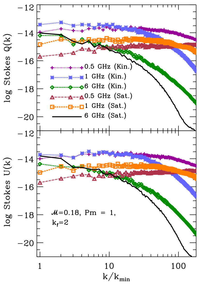
Figure 10: Power spectra of the Stokes $Q$ (top) and $U$ (bottom) at 0.5, 1 and 6 GHz in the kinematic ($t/t_{\rm ed}=2$) and saturated phase ($t/t_{\rm ed}=23$). The wavenumber is normalized in units of $k_{\rm min}=2\pi/L$.

Here, we present the power spectra of the Stokes $Q$ and $U$ parameters in Fig. 10, obtained at the native resolution of our simulations for snapshots during the kinematic and the saturated phases. The spectra for the saturated phase are obtained using maps of Stokes $Q$ and $U$ parameters at $0.5$, $1$ and $6\,{\rm GHz}$ shown in the top two rows of Fig. 12. Since Stokes $Q$ and $U$ parameters are sensitive to the orientation of magnetic fields, it is interesting to note that, although there is no mean field in our MHD simulations and the magnetic fields are turbulent, Stokes $Q$ and $U$ maps shows large-scale structures preserving their sign at higher frequencies ($\gtrsim 5\,{\rm GHz}$). This suggests that fields are locally ordered on somewhat large scales due to stretching and twisting by the fluctuation-dynamo action. Inferences about ordered magnetic fields from large-scale features in ${\rm PI}$ maps is not straightforward because it is positive definite. Signatures of large-scale features are readily seen as large power at $k\lesssim 10$ in the power spectra of Stokes $Q$ and $U$ parameters at $6\,{\rm GHz}$ for both the kinematic and the saturated stages.

At high frequencies, the power spectra of Stokes $Q$ and $U$ parameters steepens significantly for wavenumbers above $\sim 15$, for both kinematic and saturated stages of field amplification. However, the slopes of the power spectra are different for the two stages. For the kinematic phase, the slope for $k>15$ is $-3.7$, while, for the saturated phase, the slope is $-6.5$. Note that, in the presence of a telescope beam, structures are correlated within its scale, and the power spectrum will have a steeper slope by up to $\sim-4$ (Lee & Jokipii, 1975) for $k>k_{\rm beam}$, where $k_{\rm beam}$ is the corresponding wavenumber of the Gaussian beam size. Comparatively steeper slope of power spectra of Stokes $Q$ and $U$ parameters obtained at high frequencies in the saturated phase mean that the evolutionary stage of field amplification in ICM can be investigated with sufficiently high angular resolution observations.

At frequencies below about $1.5\,{\rm GHz}$, Faraday depolarization increases in the presence of turbulent fields both in the plane of the sky and along the LOS giving rise to rapid spatial fluctuations in Stokes $Q$ and $U$ parameters (see Fig. 12). This flattens their power spectra in all spatial scales for both the kinematic and saturated phases of field amplification. Thus, extracting information on the dynamo action at low frequencies ($\lesssim 1.5\,{\rm GHz}$) will be a challenging proposition.

Appendix C RM synthesis of synthetic spectro-polarimetric data

Here we outline in detail the methodology adopted to compute FD from synthetic polarized synchrotron emission using RM synthesis. To this end, we used the PYRMSYNTH package to perform RM synthesis and RM CLEAN (Brentjens & de Bruyn, 2005; Heald et al., 2009) applied to fractional Stokes $Q$ and $U$ parameters, i.e. $Q(\nu)/I_{\rm sync}(\nu)$ and $U(\nu)/I_{\rm sync}(\nu)$ from the synthetic observations. Using these, we computed FD at a spatial pixel from RM synthesis ($\rm FD_{RM\,synth}$) following the standard method of fitting the highest peak of the Faraday depth spectrum by a parabola, wherein the location of the peak provides $\rm FD_{RM\,synth}$ and the amplitude provides the fractional polarization ($p_{\rm RM\,synth}$).

The frequency coverage and the channel resolution determines the sensitivity to structures observable in the Faraday depth spectrum. For the purpose of this work, we chose two frequency settings covering the frequencies (1) $1.5\textrm{--}7\,{\rm GHz}$ with 1024 channels of $\sim 5.4$ MHz width and (2) $4.5\textrm{--}7\,{\rm GHz}$ with 512 channels of $\sim 4.88$ MHz width. The polarization parameters from RM synthesis are obtained at a frequency that corresponds to the mean of the $\lambda^{2}$-coverage, i.e. at $3.25$ and $5.6\,{\rm GHz}$ for the frequency settings (1) and (2), respectively. Following the relations given in Brentjens & de Bruyn (2005), both these frequency settings are sensitive to a similar maximum observable $\rm FD_{RM\,synth}$ of $\sim\pm 6\times 10^{5}\,{\rm rad\,m^{-2}}$ and to similar structures extending up to $\sim 1700\,{\rm rad\,m^{-2}}$ in the FD space. However, these two frequency settings have drastically different resolutions in FD space determined by the FWHM of the rotation measure spread function (RMSF). Frequency setting (1) has $\rm RMSF=91\,{\rm rad\,m^{-2}}$, and setting (2) has $\rm RMSF=1330\,{\rm rad\,m^{-2}}$.

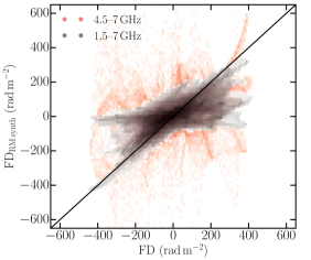
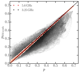
Figure 11: Pixel-by-pixel comparison of maps obtained using RM synthesis with corresponding maps obtained directly from synthetic observations of the saturated phase ($t/t_{\rm ed}=23$). Top: Variation of $\rm FD_{RM\,synth}$ with $\rm FD_{MHD}$. Red and gray points are for RM synthesis applied to synthetic observations in the frequency ranges $4.5\textrm{--}7\,{\rm GHz}$, and $1.5\textrm{--}7\,{\rm GHz}$, respectively. Bottom: Variation of $p_{\rm RM\,synth}$ with $p_{\rm MHD}$ at $5.6\,{\rm GHz}$ (red points) and at $3.25\,{\rm GHz}$ (grey points). The solid line in both the panels is the 1:1 line.

The top panel of Fig. 11 shows the pixel-wise comparison between $\rm FD_{\rm RM\,synth}$ and FD obtained from our simulation in the saturated phase ($t/t_{\rm ed}=23$), i.e. the map shown in Fig. 2. It is clear that, due to the poor resolution in FD for the high frequency coverage, $4.5\textrm{--}7\,{\rm GHz}$, $\rm FD_{RM\,synth}$ is poorly determined (shown as red points). The estimated $\rm FD_{RM\,synth}$ lies in the range $-900$ to $+800\,{\rm rad\,m^{-2}}$, and have $\sigma_{\rm FD}\approx 77\,{\rm rad\,m^{-2}}$. For the $1.5\textrm{--}7\,{\rm GHz}$ coverage, although the FD resolution is higher than that of the higher-frequency coverage, a considerable difference between $\rm FD_{RM\,synth}$ and FD is seen (grey points). In this case, $\rm FD_{RM\,synth}$ lies in the range $-425$ to $+330\,{\rm rad\,m^{-2}}$ with $\sigma_{\rm FD}\approx 73\,{\rm rad\,m^{-2}}$. In contrast, $\sigma_{\rm FD}\approx 100\,{\rm rad\,m^{-2}}$ is obtained from FD computed directly by integrating along LOS. This difference is predominantly due to the fact that the Faraday depth spectra are partially resolved showing multiple peaks, and the location of the highest peak does not necessarily correspond to the FD along the entire LOS (see Section 6). Thus the statistical properties of $\rm FD_{RM\,synth}$ for both the frequency coverage deviates significantly from the intrinsic values by up to $\pm 300\,{\rm rad\,m^{-2}}$ and manifest as spurious structures in the maps of $\rm FD_{RM\,synth}$. As a result, the power spectra computed from $\rm FD_{RM\,synth}$ maps shown in Fig. 9 deviates from the form determined by $M(k)/k$ in contrast to the power spectrum of FD map shown in Fig. 3.

The bottom panel of Fig. 11 shows the pixel-by-pixel variation of fractional polarization $p_{\rm RM\,synth}$ computed from RM synthesis applied to the two frequency ranges with $p$ computed from synthetic observations at 3.25 and $5.6\,{\rm GHz}$. At $5.6\,{\rm GHz}$, $p_{\rm RM\,synth}$ is in remarkable agreement with $p$ at better than the $\sim 2$ per cent level. This is a consequence of low Faraday rotation and depolarization at these frequencies; large RMSF means that complicated structures in the Faraday depth spectrum remains unresolved and all polarized structures in Faraday depth space are integrated within a single unresolved peak. As a result, polarization fractions are well recovered by a single peak. However, at $3.25\,{\rm GHz}$, $p_{\rm RM\,synth}$ versus $p$ has a much larger scatter and the agreement lies within a factor of about two. Notably, $p_{\rm RM\,synth}$ is in general underestimated as compared to $p$ at $3.25\,{\rm GHz}$. This is because, due to the relatively higher resolution in FD for the $1.5\textrm{--}7\,{\rm GHz}$ coverage, Faraday depth spectra are partially resolved. Therefore, the peak of the Faraday depth spectrum is somewhat lower than the expected $p$. Nonetheless, the offset of $p_{\rm RM\,synth}$ with respect to $p$ has negligible spatial dependence. Thus, the power spectra of $p_{\rm RM\,synth}$ for the two frequency ranges considered here matches the power spectra of actual $p$ very well, as seen in Fig. 9.

Appendix D Smoothed Stokes $Q$ and $U$ parameters

0.5 GHz	1 GHz	6 GHz
	Stokes $Q$
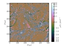
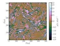
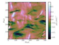
	Stokes $U$
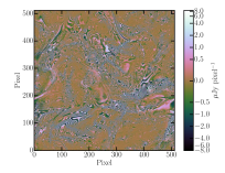
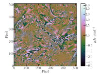
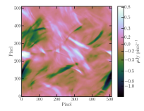
	Stokes $Q$ (smoothed 10 pixels)
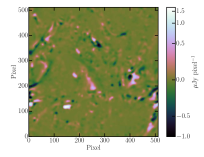
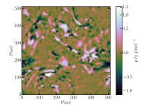
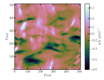
	Stokes $U$ (smoothed 10 pixels)

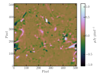
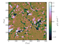
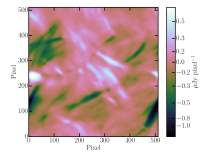
Figure 12: First row: Stokes $Q$ parameter maps in Jy pixel^-2. Second row: Stokes $U$ parameter maps in Jy pixel^-2. Third and fourth rows show the quantities after smoothing by a Gaussian kernel with FWHM 10 pixels. The left-hand, middle, and right-hand columns are at 0.5, 1, and 6 GHz, respectively, at $t/t_{\rm ed}=23$.

In order to obtain the smoothed intensity map of linear polarization presented in Fig. 6, we first convolved the Stokes $Q$ and $U$ parameter maps with a symmetric Gaussian kernel having an FWHM of $10\times 10$ pixel²; the smoothed ${\rm PI}_{\nu}$ (${\rm PI}_{\rm\nu,smooth}$) is computed as

$$PI_{\rm\nu,smooth}=\sqrt{Q_{\rm\nu,smooth}^{2}+U_{\rm\nu,smooth}^{2}}.$$ (12)

The smoothed fractional polarization ($p_{\rm\nu,smooth}$) maps presented in Fig. 6 is obtained using $p_{\rm\nu,smooth}={\rm PI}_{\rm\nu,smooth}/I_{\rm\nu,smooth}$, where $I_{\rm\nu,smooth}$ is the smoothed synchrotron intensity map. The chosen kernel size corresponds to Gaussian smoothing on a 4.25 kpc spatial scale. Smoothed images of Stokes $Q$ and $U$ parameters, $Q_{\rm\nu,smooth}$ and $U_{\rm\nu,smooth}$, respectively, at 0.5, 1 and 6 GHz are presented in the bottom two rows of Fig. 12.

At $6\,{\rm GHz}$, smoothing by a telescope beam does not significantly affect the structures observed in Stokes $Q$ and $U$ parameter images at native resolution. This is due to the presence of large-scale features in the maps of Stokes $Q$ and $U$ parameters at frequencies above $\sim 5\,{\rm GHz}$. However, at frequencies below $\sim 1.5\,{\rm GHz}$, increased Faraday rotation due to turbulent fields leads to rapid spatial fluctuations in the sign of the Stokes parameters. This results in strong depolarization within the beam that increases with decreasing frequency (see left-hand and middle panels in the bottom two rows of Fig. 12). Hence, in the presence of noise, typical observations would be sensitive to the clumpy bright and dark patches only. These correspond to the clumpy structures observed in the ${\rm PI}_{\nu}$ and $p_{\nu}$ maps shown in the bottom two rows of Fig. 6.

As seen in the left-hand panels of Fig. 12, large Faraday rotation at frequencies near $0.5\,{\rm GHz}$ introduces fluctuations in Stokes $Q$ and $U$ parameters on scales of few pixels (also seen in Fig. 10). Therefore, the structures in Stokes $Q$ and $U$ maps that are recovered when observed with a finite telescope resolution at low frequencies are drastically different as compared to their intrinsic structures, e.g. those seen at native resolution or at frequencies above $5\,{\rm GHz}$.

From this study it is obvious that depolarization within the beam introduced by Faraday rotation plays a very severe role in distorting the polarized intensity structures in the ICM as compared to beam depolarization due to turbulent magnetic fields. It should be noted that here we have investigated smoothing on a spatial scale of only 4.25 kpc, which is much smaller than the driving scale of turbulence of 256 kpc in these simulations. With currently available radio interferometers, the spatial resolutions that are typically achieved in radio continuum observations of the ICM are $\sim 30\textrm{--}50$ kpc. This will further aggravate the difficulty in the detection of polarized emission from ICM at frequencies below $\sim 1.5\,{\rm GHz}$. Hence, to maximize the chances of detecting polarized emission from ICM and robustly glean information on the nature of turbulence in it, our study shows that it is imperative to reduce the contamination from Faraday rotation by observing at frequencies higher than $5\,{\rm GHz}$.

References

- Astropy Collaboration et al. (2013) Astropy Collaboration et al., 2013, A&A, 558, A33
- Bagchi et al. (2002) Bagchi J., Enßlin T. A., Miniati F., Stalin C. S., Singh M., Raychaudhury S., Humeshkar N. B., 2002, New Astron., 7, 249
- Basu et al. (2019) Basu A., Fletcher A., Mao S. A., Burkhart B., Beck R., Schnitzeler D., 2019, Galaxies, 7, 89
- Benzi et al. (2008) Benzi R., Biferale L., Fisher R. T., Kadanoff L. P., Lamb D. Q., Toschi F., 2008, Physical Review Letters, 100, 234503
- Bernet et al. (2008) Bernet M., Miniati F., Lilly S., Kronberg P., Dessauges-Zavadsky M., 2008, Nature, 454, 302
- Bhat & Subramanian (2013) Bhat P., Subramanian K., 2013, MNRAS, 429, 2469
- Böhringer et al. (2016) Böhringer H., Chon G., Kronberg P. P., 2016, A&A, 596, A22
- Bonafede et al. (2009) Bonafede A., et al., 2009, A&A, 503, 707
- Bonafede et al. (2010) Bonafede A., Feretti L., Murgia M., Govoni F., Giovannini G., Dallacasa D., Dolag K., Taylor G. B., 2010, A&A, 513, A30
- Bonafede et al. (2015) Bonafede A., et al., 2015, in Advancing Astrophysics with the Square Kilometre Array (AASKA14). Sissa Medialab, Trieste, Italy, p. 95 (arXiv:1501.00321)
- Brandenburg & Subramanian (2005) Brandenburg A., Subramanian K., 2005, Phys. Rep., 417, 1
- Brentjens & de Bruyn (2005) Brentjens M. A., de Bruyn A. G., 2005, A&A, 441, 1217
- Brunetti & Jones (2014) Brunetti G., Jones T. W., 2014, International Journal of Modern Physics D, 23, 1430007
- Burn (1966) Burn B. J., 1966, MNRAS, 133, 67
- Carilli & Taylor (2002) Carilli C. L., Taylor G. B., 2002, ARA&A, 40, 319
- Cho & Ryu (2009) Cho J., Ryu D., 2009, ApJ, 705, L90
- Churazov et al. (2012) Churazov E., et al., 2012, MNRAS, 421, 1123
- Clarke et al. (2001) Clarke T. E., Kronberg P. P., Böhringer H., 2001, ApJ, 547, L111
- Dewdney et al. (2016) Dewdney P. et al., 2016, SKA1 System Baseline Design V2, available at: https://astronomers.skatelescope.org/wp-content/uploads/2016/05/SKA-TEL-SKO-0000002_03_SKA1SystemBaselineDesignV2.pdf, p 1
- Dolag et al. (1999) Dolag K., Bartelmann M., Lesch H., 1999, A&A, 348, 351
- Domínguez-Fernández et al. (2019) Domínguez-Fernández P., Vazza F., Brüggen M., Brunetti G., 2019, MNRAS, 486, 623
- Drury (1983) Drury L. O., 1983, Reports on Progress in Physics, 46, 973
- Eswaran & Pope (1988) Eswaran V., Pope S. B., 1988, Physics of Fluids, 31, 506
- Farnes et al. (2014) Farnes J. S., O’Sullivan S. P., Corrigan M. E., Gaensler B. M., 2014, ApJ, 795, 63
- Feretti et al. (2012) Feretti L., Giovannini G., Govoni F., Murgia M., 2012, A&ARv, 20, 54
- Fletcher & Shukurov (2006) Fletcher A., Shukurov A., 2006, MNRAS, 371, L21
- Fryxell et al. (2000) Fryxell B., et al., 2000, ApJS, 131, 273
- Govoni & Feretti (2004) Govoni F., Feretti L., 2004, International Journal of Modern Physics D, 13, 1549
- Govoni et al. (2005) Govoni F., Murgia M., Feretti L., Giovannini G., Dallacasa D., Taylor G. B., 2005, A&A, 430, L5
- Govoni et al. (2013) Govoni F., Murgia M., Xu H., Li H., Norman M. L., Feretti L., Giovannini G., Vacca V., 2013, A&A, 554, A102
- Govoni et al. (2015) Govoni F., et al., 2015, in Advancing Astrophysics with the Square Kilometre Array (AASKA14). Sissa Medialab, Trieste, Italy, p. 105 (arXiv:1501.00389)
- Haugen et al. (2004) Haugen N. E., Brandenburg A., Dobler W., 2004, Phys. Rev. E, 70, 016308
- Heald et al. (2009) Heald G., Braun R., Edmonds R., 2009, A&A, 503, 409
- Hitomi Collaboration: Aharonian et al. (2018) Hitomi Collaboration: Aharonian F., et al., 2018, PASJ, 70, 9
- Hunter (2007) Hunter J. D., 2007, Computing in Science & Engineering, 9, 90
- Jelić et al. (2015) Jelić V., et al., 2015, A&A, 583, A137
- Jelić et al. (2018) Jelić V., Prelogović D., Haverkorn M., Remeijn J., Klindžić D., 2018, A&A, 615, L3
- Kale et al. (2016) Kale R., et al., 2016, Journal of Astrophysics and Astronomy, 37, 31
- Kazantsev (1968) Kazantsev A. P., 1968, Soviet Journal of Experimental and Theoretical Physics, 26, 1031
- Kierdorf et al. (2017) Kierdorf M., Beck R., Hoeft M., Klein U., van Weeren R. J., Forman W. R., Jones C., 2017, A&A, 600, A18
- Kramer et al. (2016) Kramer M., et al., 2016, in MeerKAT Science: On the Pathway to the SKA. Sissa Medialab, Trieste, Italy, p. 3
- Laing et al. (2008) Laing R. A., Bridle A. H., Parma P., Murgia M., 2008, MNRAS, 391, 521
- Lee & Deane (2009) Lee D., Deane A. E., 2009, Journal of Computational Physics, 228, 952
- Lee & Jokipii (1975) Lee L. C., Jokipii J. R., 1975, ApJ, 196, 695
- Lee et al. (2013) Lee K.-G., et al., 2013, AJ, 145, 69
- Loi et al. (2019) Loi F., et al., 2019, MNRAS, 490, 4841
- Longair (2011) Longair M., 2011, High energy astrophysics, 3rd ed. Cambridge: Cambridge University Press
- Malik et al. (2020) Malik S., Chand H., Seshadri T. R., 2020, ApJ, 890, 132
- Marinacci et al. (2018) Marinacci F., et al., 2018, MNRAS, 480, 5113
- Miniati (2014) Miniati F., 2014, ApJ, 782, 21
- Miniati (2015) Miniati F., 2015, ApJ, 800, 60
- Miyoshi & Kusano (2005) Miyoshi T., Kusano K., 2005, Journal of Computational Physics, 208, 315
- Murgia et al. (2004) Murgia M., Govoni F., Feretti L., Giovannini G., Dallacasa D., Fanti R., Taylor G. B., Dolag K., 2004, A&A, 424, 429
- On et al. (2019) On A. Y. L., Chan J. Y. H., Wu K., Saxton C. J., van Driel-Gesztelyi L., 2019, MNRAS, 490, 1697
- Planck Collaboration et al. (2020) Planck Collaboration VI, 2020, A&A, 641, A6
- Price-Whelan et al. (2018) Price-Whelan A. M., et al., 2018, AJ, 156, 123
- Roh et al. (2019) Roh S., Ryu D., Kang H., Ha S., Jang H., 2019, ApJ, 883, 138
- Roy et al. (2016) Roy S., Sur S., Subramanian K., Mangalam A., Seshadri T. R., Chand H., 2016, Journal of Astrophysics and Astronomy, 37, 42
- Sanders & Fabian (2013) Sanders J. S., Fabian A. C., 2013, MNRAS, 429, 2727
- Sanders et al. (2011) Sanders J. S., Fabian A. C., Smith R. K., 2011, MNRAS, 410, 1797
- Sarazin (1988) Sarazin C. L., 1988, X-Ray Emission From Clusters Of Galaxies. Cambridge Univ. Press, Cambridge
- Schekochihin et al. (2004) Schekochihin A. A., Cowley S. C., Taylor S. F., Maron J. L., McWilliams J. C., 2004, ApJ, 612, 276
- Schuecker et al. (2004) Schuecker P., Finoguenov A., Miniati F., Böhringer H., Briel U. G., 2004, A&A, 426, 387
- Seta et al. (2020) Seta A., Bushby P. J., Shukurov A., Wood T. S., 2020, Physical Review Fluids, 5, 043702
- Shi et al. (2018) Shi X., Nagai D., Lau E. T., 2018, MNRAS, 481, 1075
- Shukurov & Berkhuijsen (2003) Shukurov A., Berkhuijsen E. M., 2003, MNRAS, 342, 496
- Sokoloff et al. (1998) Sokoloff D., Bykov A., Shukurov A., Berkhuijsen E., Beck R., Poezd A., 1998, MNRAS, 299, 189
- Subramanian et al. (2006) Subramanian K., Shukurov A., Haugen N. E. L., 2006, MNRAS, 366, 1437
- Sur (2019) Sur S., 2019, MNRAS, 488, 3439
- Sur et al. (2018) Sur S., Bhat P., Subramanian K., 2018, MNRAS, 475, L72
- Thompson et al. (2017) Thompson A. R., Moran J. M., Swenson G. W., 2017, Further Imaging Techniques. Springer. Cham, pp 551, doi:10.1007/978-3-319-44431-4_11
- Tribble (1991) Tribble P. C., 1991, MNRAS, 250, 726
- Vacca et al. (2010) Vacca V., Murgia M., Govoni F., Feretti L., Giovannini G., Orrù E., Bonafede A., 2010, A&A, 514, A71
- van der Walt et al. (2011) van der Walt S., Colbert S. C., Varoquaux G., 2011, Computing in Science Engineering, 13, 22
- van Weeren et al. (2019) van Weeren R. J., de Gasperin F., Akamatsu H., Brüggen M., Feretti L., Kang H., Stroe A., Zandanel F., 2019, Space Sci. Rev., 215, 16
- Vazza et al. (2018) Vazza F., Brunetti G., Brüggen M., Bonafede A., 2018, MNRAS, 474, 1672
- Vogt & Enßlin (2003) Vogt C., Enßlin T. A., 2003, A&A, 412, 373
- Waelkens et al. (2009) Waelkens A. H., Schekochihin A. A., Enßlin T. A., 2009, MNRAS, 398, 1970
- Wardle & Kronberg (1974) Wardle J. F. C., Kronberg P. P., 1974, ApJ, 194, 249
- Xu et al. (2009) Xu H., Li H., Collins D. C., Li S., Norman M. L., 2009, ApJ, 698, L14
- Xu et al. (2011) Xu H., Li H., Collins D. C., Li S., Norman M. L., 2011, ApJ, 739, 77
- Xu et al. (2012) Xu H., et al., 2012, ApJ, 759, 40
- Zaroubi et al. (2015) Zaroubi S., et al., 2015, MNRAS, 454, L46
- Zeldovich et al. (1990) Zeldovich Y. B., Ruzmaikin A. A., Sokoloff D. D., 1990, The almighty chance, doi:10.1142/0862.
- Zhuravleva et al. (2019) Zhuravleva I., Churazov E., Schekochihin A. A., Allen S. W., Vikhlinin A., Werner N., 2019, Nature Astronomy, 3, 832