Federated Composite Optimization

Abstract

Federated Learning (FL) is a distributed learning paradigm that scales on-device learning collaboratively and privately. Standard FL algorithms such as FedAvg are primarily geared towards smooth unconstrained settings. In this paper, we study the Federated Composite Optimization (FCO) problem, in which the loss function contains a non-smooth regularizer. Such problems arise naturally in FL applications that involve sparsity, low-rank, monotonicity, or more general constraints. We first show that straightforward extensions of primal algorithms such as FedAvg are not well-suited for FCO since they suffer from the “curse of primal averaging,” resulting in poor convergence. As a solution, we propose a new primal-dual algorithm, Federated Dual Averaging (FedDualAvg), which by employing a novel server dual averaging procedure circumvents the curse of primal averaging. Our theoretical analysis and empirical experiments demonstrate that FedDualAvg outperforms the other baselines.

1 Introduction

Federated Learning (FL, Konečnỳ et al. 2015; McMahan et al. 2017) is a novel distributed learning paradigm in which a large number of clients collaboratively train a shared model without disclosing their private local data. The two most distinct features of FL, when compared to classic distributed learning settings, are (1) heterogeneity in data amongst the clients and (2) very high cost to communicate with a client. Due to these aspects, classic distributed optimization algorithms have been rendered ineffective in FL settings (Kairouz et al., 2019). Several algorithms specifically catered towards FL settings have been proposed to address these issues. The most prominent amongst them is Federated Averaging (FedAvg) algorithm, which by employing local SGD updates, significantly reduces the communication overhead under moderate client heterogeneity. Several follow-up works have focused on improving the FedAvg in various ways (e.g., Li et al. 2020a; Karimireddy et al. 2020; Reddi et al. 2020; Yuan and Ma 2020).

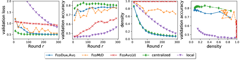
Figure 1: Results on sparse ($\ell_{1}$-regularized) logistic regression for a federated fMRI dataset based on (Haxby, 2001). centralized corresponds to training on the centralized dataset gathered from all the training clients. local corresponds to training on the local data from only one training client without communication. FedAvg ($\partial$) corresponds to running FedAvg algorithms with subgradient in lieu of SGD to handle the non-smooth $\ell_{1}$-regularizer. FedMiD is another straightforward extension of FedAvg running local proximal gradient method (see Section 3.1 for details). We show that using our proposed algorithm FedDualAvg, one can 1) achieve performance comparable to the centralized baseline without the need to gather client data, and 2) significantly outperforms the local baseline on the isolated data and the FedAvg baseline. See Section 5.3 for details.

Existing FL research primarily focuses on the unconstrained smooth objectives; however, many FL applications involve non-smooth objectives. Such problems arise naturally in the context of regularization (e.g., sparsity, low-rank, monotonicity, or additional constraints on the model). For instance, consider the problem of cross-silo biomedical FL, where medical organizations collaboratively aim to learn a global model on their patients’ data without sharing. In such applications, sparsity constraints are of paramount importance due to the nature of the problem as it involves only a few data samples (e.g., patients) but with very high dimensions (e.g., fMRI scans). For the purpose of illustration, in Fig. 1, we present results on a federated sparse ($\ell_{1}$-regularized) logistic regression task for an fMRI dataset (Haxby, 2001). As shown, using a federated approach that can handle non-smooth objectives enables us to find a highly accurate sparse solution without sharing client data.

In this paper, we propose to study the Federated Composite Optimization (FCO) problem. As in standard FL, the losses are distributed to $M$ clients. In addition, we assume all the clients share the same, possibly non-smooth, non-finite regularizer $\psi$. Formally, (FCO) is of the following form

$$\min_{w\in\mathbb{R}^{d}}\Phi(w):=F(w)+\psi(w):=\frac{1}{M}\sum_{m=1}^{M}F_{m}(w)+\psi(w),$$ (FCO)

where $F_{m}(w):=\operatorname{\mathbb{E}}_{\xi^{m}\sim\mathcal{D}_{m}}f(w;\xi^{m})$ is the loss at the $m$-th client, assuming $\mathcal{D}_{m}$ is its local data distribution. We assume that each client $m$ can access $\nabla f(w;\xi^{m})$ by drawing independent samples $\xi^{m}$ from its local distribution $\mathcal{D}_{m}$. Common examples of $\psi(w)$ include $\ell_{1}$-regularizer or more broadly $\ell_{p}$-regularizer, nuclear-norm regularizer (for matrix variable), total variation (semi-)norm, etc. The (FCO) reduces to the standard federated optimization problem if $\psi\equiv 0$. The (FCO) also covers the constrained federated optimization if one takes $\psi$ to be the following constraint characteristics $\chi_{\mathcal{C}}(w):=\begin{cases}0&\text{if $w\in\mathcal{C}$},\\ +\infty&\text{if $w\notin\mathcal{C}$}.\end{cases}$

Standard FL algorithms such as FedAvg (see Algorithm 1) and its variants (e.g., Li et al. 2020a; Karimireddy et al. 2020) are primarily tailored to smooth unconstrained settings, and are therefore, not well-suited for FCO. The most straightforward extension of FedAvg towards (FCO) is to apply local subgradient method (Shor, 1985) in lieu of SGD. This approach is largely ineffective due to the intrinsic slow convergence of subgradient approach (Boyd et al., 2003), which is also demonstrated in Fig. 1 (marked FedAvg ($\partial$)).

A more natural extension of FedAvg is to replace the local SGD with proximal SGD (Parikh and Boyd 2014, a.k.a. projected SGD for constrained problems), or more generally, mirror descent Duchi et al. (2010). We refer to this algorithm as Federated Mirror Descent (FedMiD, see Algorithm 2). The most noticeable drawback of a primal-averaging method like FedMiD is the “curse of primal averaging,” where the desired regularization of FCO may be rendered completely ineffective due to the server averaging step typically used in FL. For instance, consider a $\ell_{1}$-regularized logistic regression setting. Although each client is able to obtain a sparse solution, simply averaging the client states will inevitably yield a dense solution. See Fig. 2 for an illustrative example.

Figure 2: Illustration of “curse of primal averaging”. While each client of FedMiD can locate a sparse solution, simply averaging them will yield a much denser solution on the server side.

To overcome this challenge, we propose a novel primal-dual algorithm named Federated Dual Averaging (FedDualAvg, see Algorithm 3). Unlike FedMiD (or its precursor FedAvg), the server averaging step of FedDualAvg operates in the dual space instead of the primal. Locally, each client runs dual averaging algorithm (Nesterov, 2009) by tracking of a pair of primal and dual states. During communication, the dual states are averaged across the clients. Thus, FedDualAvg employs a novel double averaging procedure — averaging of dual states across clients (as in FedAvg), and the averaging of gradients in dual space (as in the sequential dual averaging). Since both levels of averaging operate in the dual space, we can show that FedDualAvg provably overcomes the curse of primal averaging. Specifically, we prove that FedDualAvg can attain significantly lower communication complexity when deployed with a large client learning rate.

Contributions.

In light of the above discussion, let us summarize our key contributions below:

• We propose a generalized federated learning problem, namely Federated Composite Optimization (FCO), with non-smooth regularizers and constraints.

• We first propose a natural extension of FedAvg, namely Federated Mirror Descent (FedMiD). We show that FedMiD can attain the mini-batch rate in the small client learning rate regime (Section 4.1). We argue that FedMiD may suffer from the effect of “curse of primal averaging,” which results in poor convergence, especially in the large client learning rate regime (Section 3.2).

• We propose a novel primal-dual algorithm named Federated Dual Averaging (FedDualAvg), which provably overcomes the curse of primal averaging (Section 3.3). Under certain realistic conditions, we show that by virtue of “double averaging” property, FedDualAvg can have significantly lower communication complexity (Section 4.2).

• We demonstrate the empirical performance of FedMiD and FedDualAvg on various tasks, including $\ell_{1}$-regularization, nuclear-norm regularization, and various constraints in FL (Section 5).

Notations.

We use $[n]$ to denote the set $\{1,\ldots,n\}$. We use $\langle\cdot,\cdot\rangle$ to denote the inner product, $\|\cdot\|$ to denote an arbitrary norm, and $\|\cdot\|_{*}$ to denote its dual norm, unless otherwise specified. We use $\|\cdot\|_{2}$ to denote the $\ell_{2}$ norm of a vector or the operator norm of a matrix, and $\|\cdot\|_{A}$ to denote the vector norm induced by positive definite matrix $A$, namely $\|w\|_{A}:=\sqrt{\left\langle w,Aw\right\rangle}$. For any convex function $g(w)$, we use $g^{*}(z)$ to denote its convex conjugate $g^{*}(z):=\sup_{w\in\mathbb{R}^{d}}\{\langle z,w\rangle-g(w)\}$. We use $w^{\star}$ to denote the optimum of the problem (FCO). We use $\mathcal{O},\Theta$ to hide multiplicative absolute constants only and $x\lesssim y$ to denote $x=\mathcal{O}(y)$.

1.1 Additional Related Work

Federated Learning.

Recent years have witnessed a growing interest in various aspects of Federated Learning. The early analysis of FedAvg preceded the inception of Federated Learning, which was studied under the names of parallel SGD and local SGD (Zinkevich et al., 2010; Zhou and Cong, 2018) Early results on FedAvg mostly focused on the “one-shot” averaging case, in which the clients are only synchronized once at the end of the procedure (e.g., Mcdonald et al. 2009; Shamir and Srebro 2014; Rosenblatt and Nadler 2016; Jain et al. 2018; Godichon-Baggioni and Saadane 2020). The first analysis of general FedAvg was established by (Stich, 2019) for the homogeneous client dataset. This result was improved by (Haddadpour et al., 2019b; Khaled et al., 2020; Woodworth et al., 2020b; Yuan and Ma, 2020) via tighter analysis and accelerated algorithms. FedAvg has also been studied for non-convex objectives (Zhou and Cong, 2018; Haddadpour et al., 2019a; Wang and Joshi, 2018; Yu and Jin, 2019; Yu et al., 2019a, b). For heterogeneous clients, numerous recent papers (Haddadpour et al., 2019b; Khaled et al., 2020; Li et al., 2020b; Koloskova et al., 2020; Woodworth et al., 2020a) studied the convergence of FedAvg under various notions of heterogeneity measure. Other variants of FedAvg have been proposed to overcome heterogeneity (e.g., Mohri et al. 2019; Zhang et al. 2020; Li et al. 2020a; Wang et al. 2020; Karimireddy et al. 2020; Reddi et al. 2020; Pathak and Wainwright 2020; Al-Shedivat et al. 2021). A recent line of work has studied the behavior of Federated algorithms for personalized multi-task objectives (Smith et al., 2017; Hanzely et al., 2020; T. Dinh et al., 2020; Deng et al., 2020) and meta-learning objectives (Fallah et al., 2020; Chen et al., 2019; Jiang et al., 2019). Federated Learning techniques have been successfully applied in a broad range of practical applications (Hard et al., 2018; Hartmann et al., 2019; Hard et al., 2020). We refer readers to (Kairouz et al., 2019) for a comprehensive survey of the recent advances in Federated Learning. However, none of the aforementioned work allows for non-smooth or constrained problems such as (FCO). To the best of our knowledge, the present work is the first work that studies non-smooth or constrained problems in Federated settings.

Shortly after the initial preprint release of the present work, Tong et al. (2020) proposed a related federated $\ell_{0}$-constrained problem (which does not belong to FCO due to the non-convexity of $\ell_{0}$), and two algorithms to solve (similar to FedMiD (-OSP) but with hard-thresholding instead). As in most hard-thresholding work, the convergence is weaker since it depends on the sparsity level $\tau$ (worsens as $\tau$ gets tighter).

Composite Optimization, Dual Averaging, and Mirror Descent.

Composite optimization has been a classic problem in convex optimization, which covers a variety of statistical inference, machine learning, signal processing problems. Mirror Descent (MD, a generalization of proximal gradient method) and Dual Averaging (DA, a.k.a. lazy mirror descent) are two representative algorithms for convex composite optimization. The Mirror Descent (MD) method was originally introduced by Nemirovski and Yudin (1983) for the constrained case and reinterpreted by Beck and Teboulle (2003). MD was generalized to the composite case by Duchi et al. (2010) under the name of Comid, though numerous preceding work had studied the special case of Comid under a variety of names such as gradient mapping (Nesterov, 2013), forward-backward splitting method (FOBOS,Duchi and Singer 2009), iterative shrinkage and thresholding (ISTA, Daubechies et al. 2004), and truncated gradient (Langford et al., 2009). The Dual Averaging (DA) method was introduced by Nesterov (2009) for the constrained case, which is also known as Lazy Mirror Descent in the literature (Bubeck, 2015). The DA method was generalized to the composite (regularized) case by (Xiao, 2010; Dekel et al., 2012) under the name of Regularized Dual Averaging, and extended by recent works (Flammarion and Bach, 2017; Lu et al., 2018) to account for non-Euclidean geometry induced by an arbitrary distance-generating function $h$. DA also has its roots in online learning (Zinkevich, 2003), and is related to the follow-the-regularized-leader (FTRL) algorithms (McMahan, 2011). Other variants of MD or DA (such as delayed / skipped proximal step) have been investigated to mitigate the expensive proximal oracles (Mahdavi et al., 2012; Yang et al., 2017). We refer readers to (Flammarion and Bach, 2017; Diakonikolas and Orecchia, 2019) for more detailed discussions on the recent advances of MD and DA.

Classic Decentralized Consensus Optimization.

A related distributed setting is the decentralized consensus optimization, also known as multi-agent optimization or optimization over networks in the literature (Nedich, 2015). Unlike the federated settings, in decentralized consensus optimization, each client can communicate every iteration, but the communication is limited to its graphic neighborhood. Standard algorithms for unconstrained consensus optimization include decentralized (sub)gradient methods (Nedic and Ozdaglar, 2009; Yuan et al., 2016) and EXTRA (Shi et al., 2015a; Mokhtari and Ribeiro, 2016). For constrained or composite consensus problems, people have studied both mirror-descent type methods (with primal consensus), e.g., (Sundhar Ram et al., 2010; Shi et al., 2015b; Rabbat, 2015; Yuan et al., 2018, 2020); and dual-averaging type methods (with dual consensus), e.g., (Duchi et al., 2012; Tsianos et al., 2012; Tsianos and Rabbat, 2012; Liu et al., 2018). In particular, the distributed dual averaging (Duchi et al., 2012) has gained great popularity since its dual consensus scheme elegantly handles the constraints, and overcomes the technical difficulties of primal consensus, as noted by the original paper. We identify that while the federated settings share certain backgrounds with the decentralized consensus optimization, the motivations, techniques, challenges, and results are quite dissimilar due to the fundamental difference of communication protocol, as noted by (Kairouz et al., 2019). We refer readers to (Nedich, 2015) for a more detailed introduction to the classic decentralized consensus optimization.

2 Preliminaries

In this section, we review the necessary background for composite optimization and federated learning. A detailed technical exposition of these topics is relegated to Appendix B.

2.1 Composite Optimization

Composite optimization covers a variety of statistical inference, machine learning, signal processing problems. Standard (non-distributed) composite optimization is defined as

$$\min_{w\in\mathbb{R}^{d}}\quad\operatorname{\mathbb{E}}_{\xi\sim\mathcal{D}}f(w;\xi)+\psi(w),$$ (CO)

where $\psi$ is a non-smooth, possibly non-finite regularizer.

Proximal Gradient Method.

A natural extension of SGD for (CO) is the following proximal gradient method (PGM):

$$w_{t+1}\leftarrow\operatorname{\mathbf{prox}}_{\eta\psi}\left(w_{t}-\eta\nabla f(w_{t};\xi_{t})\right)=\operatorname*{arg\,min}_{w}\left(\eta\langle\nabla f(w_{t};\xi_{t}),w\rangle+\frac{1}{2}\|w-w_{t}\|_{2}^{2}+\eta\psi(w)\right).$$ (2.1)

The sub-problem Eq. 2.1 can be motivated by optimizing a quadratic upper bound of $f$ together with the original $\psi$. This problem can often be efficiently solved by virtue of the special structure of $\psi$. For instance, one can verify that PGM reduces to projected gradient descent if $\psi$ is a constraint characteristic ${\chi}_{\mathcal{C}}$, soft thresholding if $\psi(w)=\lambda\|w\|_{1}$, or weight decay if $\psi(w):=\lambda\|w\|_{2}^{2}$.

Mirror Descent / Bregman-PGM.

PGM can be generalized to the Bregman-PGM if one replaces the Euclidean proximity term by the general Bregman divergence, namely

$$w_{t+1}\leftarrow\operatorname*{arg\,min}_{w}\left(\eta\left\langle\nabla f(w_{t};\xi_{t}),w\right\rangle+\eta\psi(w)+D_{h}(w,w_{t})\right),$$ (2.2)

where $h$ is a strongly convex distance-generating function, $D_{h}$ is the Bregman divergence which reduces to Euclidean distance if one takes $h(w)=\frac{1}{2}\|w\|_{2}^{2}$. We will still refer to this step as a proximal step for ease of reference. This general formulation (2.2) enables an equivalent primal-dual interpretation:

$$w_{t+1}\leftarrow\nabla(h+\eta\psi)^{*}(\nabla h(w_{t})-\nabla f(w_{t};\xi_{t})).$$ (2.3)

A common interpretation of (2.3) is to decompose it into the following three sub-steps (Nemirovski and Yudin, 1983):

1. Apply $\nabla h$ to carry $w_{t}$ to a dual state (denoted as $z_{t}$)

2. Update $z_{t}$ to $y_{t+1}$ with the gradient queried at $w_{t}$.

3. Map $y_{t+1}$ back to primal via $\nabla(h+\eta\psi)^{*}$

This formulation is known as the composite objective mirror descent (Comid, Duchi et al. 2010), or simply mirror descent in the literature (Flammarion and Bach, 2017).

Dual Averaging.

An alternative approach for (CO) is the following dual averaging algorithm (Nesterov, 2009):

$$z_{t+1}\leftarrow z_{t}-\eta\nabla f\left(\nabla(h+\eta t\psi)^{*}(z_{t});\xi_{t}\right).$$ (2.4)

Similarly, we can decompose (2.4) into two sub-steps:

1. Apply $\nabla(h+\eta t\psi)^{*}$ to map dual state $z_{t}$ to primal $w_{t}$. Note that this sub-step can be reformulated into

   $$w_{t}=\operatorname*{arg\,min}_{w}\left(\left\langle-z_{t},w\right\rangle+\eta t\psi(w)+h(w)\right),$$ (2.5)

   which allows for efficient computation for many $\psi$, as in PGM.

2. Update $z_{t}$ to $z_{t+1}$ with the gradient queried at $w_{t}$.

Dual averaging is also known as the “lazy” mirror descent algorithm (Bubeck, 2015) since it skips the forward mapping $(\nabla h)$ step. Theoretically, mirror descent and dual averaging often share the similar convergence rates for sequential (CO) (e.g., for smooth convex $f$, c.f. Flammarion and Bach 2017).

Remark.

There are other algorithms that are popular for certain types of (CO) problems. For example, Frank-Wolfe method (Frank and Wolfe, 1956; Jaggi, 2013) solves constrained optimization with a linear optimization oracle. Smoothing method (Nesterov, 2005) can also handle non-smoothness in objectives, but is in general less efficient than specialized CO algorithms such as dual averaging (c.f., Nesterov 2018). In this work, we mostly focus on Mirror Descent and Dual Averaging algorithms since they only employ simple proximal oracles such as projection and soft-thresholding.

2.2 Federated Averaging

Federated Averaging (FedAvg, McMahan et al. 2017) is the de facto standard algorithm for Federated Learning with unconstrained smooth objectives (namely $\psi=0$ for (FCO)). In this work, we follow the exposition of (Reddi et al., 2020) which splits the client learning rate and server learning rate, offering more flexibility (see Algorithm 1).

FedAvg involves a series of rounds in which each round consists of a client update phase and server update phase. We denote the total number of rounds as $R$. At the beginning of each round $r$, a subset of clients $\mathcal{S}_{r}$ are sampled from the client pools of size $M$. The server state is then broadcast to the sampled client as the client initialization. During the client update phase (highlighted in blue shade), each sampled client runs local SGD for $K$ steps with client learning rate $\eta_{\mathrm{c}}$ with their own data. We use $w_{r,k}^{m}$ to denote the $m$-th client state at the $k$-th local step of the $r$-th round. During the server update phase, the server averages the updates of the sampled clients and treats it as a pseudo-anti-gradient $\Delta_{r}$ (Line 9). The server then takes a server update step to update its server state with server learning rate $\eta_{\mathrm{s}}$ and the pseudo-anti-gradient $\Delta_{r}$ (Line 10).

Algorithm 1 Federated Averaging (FedAvg)

1:  procedure FedAvg ($w_{0},\eta_{\mathrm{c}},\eta_{\mathrm{s}}$)

2:  for $r=0,\ldots,R-1$ do

3:    sample a subset of clients $\mathcal{S}_{r}\subseteq[M]$

4:    on client for  $m\in\mathcal{S}_{r}$ in parallel do

5:      $w_{r,0}^{m}\leftarrow w_{r}$ $\vartriangleright$ broadcast client initialization

6:      for $k=0,\ldots,K-1$ do

7:         $g_{r,k}^{m}\leftarrow\nabla f(w_{r,k}^{m};\xi_{r,k}^{m})$ $\vartriangleright$ query gradient

8:         $w_{r,k+1}^{m}\leftarrow w_{r,k}^{m}-\eta_{\mathrm{c}}\cdot g_{r,k}^{m}$ $\vartriangleright$ client update

9:    $\Delta_{r}=\frac{1}{|\mathcal{S}_{r}|}\sum_{m\in\mathcal{S}_{r}}(w_{r,K}^{m}-w_{r,0}^{m})$

10:    $w_{r+1}\leftarrow w_{r}+\eta_{\mathrm{s}}\cdot\Delta_{r}$ $\vartriangleright$ server update

3 Proposed Algorithms for FCO

In this section, we explore the possible solutions to approach (FCO). As mentioned earlier, existing FL algorithms such as FedAvg and its variants do not solve (FCO). Although it is possible to apply FedAvg to non-smooth settings by using subgradient in place of the gradient, such an approach is usually ineffective owing to the intrinsic slow convergence of subgradient methods (Boyd et al., 2003).

3.1 Federated Mirror Descent (FedMiD)

A more natural extension of FedAvg towards (FCO) is to replace the local SGD steps in FedAvg with local proximal gradient (mirror descent) steps (2.3). The resulting algorithm, which we refer to as Federated Mirror Descent (FedMiD), is outlined in Algorithm 2.

Algorithm 2 Federated Mirror Descent (FedMiD)

1:  procedure FedMiD ($w_{0},\eta_{\mathrm{c}},\eta_{\mathrm{s}}$)

2:  for $r=0,\ldots,R-1$ do

3:    sample a subset of clients $\mathcal{S}_{r}\subseteq[M]$

4:    on client for  $m\in\mathcal{S}_{r}$ in parallel do

5:      $w_{r,0}^{m}\leftarrow w_{r}$ $\vartriangleright$ broadcast primal initialization

6:      for $k=0,\ldots,K-1$ do

7:         $g_{r,k}^{m}\leftarrow\nabla f(w_{r,k}^{m};\xi_{r,k}^{m})$ $\vartriangleright$ query gradient

8:         $w_{r,k+1}^{m}\leftarrow\nabla(h+\eta_{\mathrm{c}}\psi)^{*}(\nabla h(w_{r,k}^{m})-\eta_{\mathrm{c}}\cdot g_{r,k}^{m})$ $\vartriangleright$ client update

9:    $\Delta_{r}=\frac{1}{|\mathcal{S}_{r}|}\sum_{m\in\mathcal{S}_{r}}(w_{r,K}^{m}-w_{r,0}^{m})$

10:    $w_{r+1}\leftarrow\nabla(h+\eta_{\mathrm{s}}\eta_{\mathrm{c}}K\psi)^{*}(\nabla h(w_{r})+\eta_{\mathrm{s}}\cdot\Delta_{r})$ $\vartriangleright$ server update

Specifically, we make two changes compared to FedAvg:

• The client local SGD steps in FedAvg are replaced with proximal gradient steps (Line 8).

• The server update step is replaced with another proximal step (Line 10).

As a sanity check, for constrained (FCO) with $\psi=\chi_{\mathcal{C}}$, if one takes server learning rate $\eta_{\mathrm{s}}=1$ and Euclidean distance $h(w)=\frac{1}{2}\|w\|_{2}^{2}$, FedMiD will simply reduce to the following parallel projected SGD with periodic averaging:

1. Each sampled client runs $K$ steps of projected SGD following $w_{r,k+1}^{m}\leftarrow\mathbf{Proj}_{\mathcal{C}}(w_{r,k}^{m}-\eta_{\mathrm{c}}g_{r,k}^{m})$.

2. After $K$ local steps, the server simply average the client states following $w_{r+1}\leftarrow\frac{1}{|\mathcal{S}_{r}|}\sum_{m\in\mathcal{S}_{r}}w_{r,K}^{m}$.

3.2 Limitation of FedMiD: Curse of Primal Averaging

Despite its simplicity, FedMiD exhibits a major limitation, which we refer to as “curse of primal averaging”: the server averaging step in FedMiD may severely impede the optimization progress. To understand this phenomenon, let us consider the following two illustrative examples:

• Constrained problem: Suppose the optimum of the aforementioned constrained problem resides on a non-flat boundary $\mathcal{C}$. Even when each client is able to obtain a local solution on the boundary, the average of them will almost surely be off the boundary (and hence away from the optimum) due to the curvature.

• Federated $\ell_{1}$-regularized logistic regression problem: Suppose each client obtains a local sparse solution, simply averaging them across clients will invariably yield a non-sparse solution.

As we will see theoretically (Section 4) and empirically (Section 5), the “curse of primal averaging” indeed hampers the performance of FedMiD.

3.3 Federated Dual Averaging (FedDualAvg)

Before we look into the solution of the curse of primal averaging, let us briefly investigate the cause of this effect. Recall that in standard smooth FL settings, server averaging step is helpful because it implicitly pools the stochastic gradients and thereby reduces the variance (Stich, 2019). In FedMiD, however, the server averaging operates on the post-proximal primal states, but the gradient is updated in the dual space (recall the primal-dual interpretation of mirror descent in Section 2.1). This primal/dual mismatch creates an obstacle for primal averaging to benefit from the pooling of stochastic gradients in dual space. This thought experiment suggests the importance of aligning the gradient update and server averaging.

Building upon this intuition, we propose a novel primal-dual algorithm, named Federated Dual Averaging (FedDualAvg, Algorithm 3), which provably addresses the curse of primal averaging. The major novelty of FedDualAvg, in comparison with FedMiD or its precursor FedAvg, is to operate the server averaging in the dual space instead of the primal. This facilitates the server to aggregate the gradient information since the gradients are also accumulated in the dual space.

Formally, each client maintains a pair of primal and dual states $(w_{r,k}^{m},z_{r,k}^{m})$. At the beginning of each client update round, the client dual state is initialized with the server dual state. During the client update stage, each client runs dual averaging steps following (2.4) to update its primal and dual state (highlighted in blue shade). The coefficient of $\psi$, namely $\tilde{\eta}_{r,k}$, is to balance the contribution from $F$ and $\psi$. At the end of each client update phase, the dual updates (instead of primal updates) are returned to the server. The server then averages the dual updates of the sampled clients and updates the server dual state.

Algorithm 3 Federated Dual Averaging (FedDualAvg)

1:  procedure FedDualAvg ($w_{0},\eta_{\mathrm{c}},\eta_{\mathrm{s}}$)

2:  $z_{0}\leftarrow\nabla h(w_{0})$ $\vartriangleright$ server dual initialization

3:  for $r=0,\ldots,R-1$ do

4:    sample a subset of clients $\mathcal{S}_{r}\subseteq[M]$

5:    on client for  $m\in\mathcal{S}_{r}$ in parallel do

6:      $z_{r,0}^{m}\leftarrow z_{r}$ $\vartriangleright$ broadcast dual initialization

7:      for $k=0,\ldots,K-1$ do

8:         $\tilde{\eta}_{r,k}\leftarrow\eta_{\mathrm{s}}\eta_{\mathrm{c}}rK+\eta_{\mathrm{c}}k$

9:         $w_{r,k}^{m}\leftarrow\nabla(h+\tilde{\eta}_{r,k}\psi)^{*}(z_{r,k}^{m})$ $\vartriangleright$ retrieve primal

10:         $g_{r,k}^{m}\leftarrow\nabla f(w_{r,k}^{m};\xi_{r,k}^{m})$ $\vartriangleright$ query gradient

11:         $z_{r,k+1}^{m}\leftarrow z_{r,k}^{m}-\eta_{\mathrm{c}}g_{r,k}^{m}$ $\vartriangleright$ client dual update

12:    $\Delta_{r}=\frac{1}{|\mathcal{S}_{r}|}\sum_{m\in\mathcal{S}_{r}}(z_{r,K}^{m}-z_{r,0}^{m})$

13:    $z_{r+1}\leftarrow z_{r}+\eta_{\mathrm{s}}\Delta_{r}$ $\vartriangleright$ server dual update

14:    $w_{r+1}\leftarrow\nabla(h+\eta_{\mathrm{s}}\eta_{\mathrm{c}}(r+1)K\psi)^{*}(z_{r+1})$ $\vartriangleright$ (optional) retrieve server primal state

We observe that the averaging in FedDualAvg is two-fold: (1) averaging of gradients in dual space within a client and (2) averaging of dual states across clients at the server. As we shall see shortly in our theoretical analysis, this novel “double” averaging of FedDualAvg in the non-smooth case enables lower communication complexity and faster convergence of FedDualAvg under realistic assumptions.

4 Theoretical Results

In this section, we demonstrate the theoretical results of FedMiD and FedDualAvg. We assume the following assumptions throughout the paper. The convex analysis definitions in Assumption 1 are reviewed in Appendix B.

Assumption 1.

Let $\|\cdot\|$ be a norm and $\|\cdot\|_{*}$ be its dual.

1. $\psi:\mathbb{R}^{d}\to\mathbb{R}\cup\{+\infty\}$ is a closed convex function with closed $\operatorname{\mathbf{dom}}\psi$. Assume that $\Phi(w)=F(w)+\psi(w)$ attains a finite optimum at $w^{\star}\in\operatorname{\mathbf{dom}}\psi$.

2. $h:\mathbb{R}^{d}\to\mathbb{R}\cup\{+\infty\}$ is a Legendre function that is 1-strongly-convex w.r.t. $\|\cdot\|$. Assume $\operatorname{\mathbf{dom}}h\supset\operatorname{\mathbf{dom}}\psi$.

3. $f(\cdot,\xi):\mathbb{R}^{d}\to\mathbb{R}$ is a closed convex function that is differentiable on $\operatorname{\mathbf{dom}}\psi$ for any fixed $\xi$. In addition, $f(\cdot,\xi)$ is $L$-smooth w.r.t. $\|\cdot\|$ on $\operatorname{\mathbf{dom}}\psi$, namely for any $u,w\in\operatorname{\mathbf{dom}}\psi$,

   $$f(u;\xi)\leq f(w;\xi)+\left\langle\nabla f(w;\xi),u-w\right\rangle+\frac{1}{2}L\|u-w\|^{2}.$$ (4.1)

4. $\nabla f$ has $\sigma^{2}$-bounded variance over $\mathcal{D}_{m}$ under $\|\cdot\|_{*}$ within $\operatorname{\mathbf{dom}}\psi$, namely for any $w\in\operatorname{\mathbf{dom}}\psi$,

   $$\operatorname{\mathbb{E}}_{\xi\sim\mathcal{D}_{m}}\left\|\nabla f(w,\xi)-\nabla F_{m}(w)\right\|_{*}^{2}\leq\sigma^{2},\text{ for any $m\in[M]$}$$ (4.2)

5. Assume that all the $M$ clients participate in the client updates for every round, namely $\mathcal{S}_{r}=[M]$.

Assumption 1(a) & (b) are fairly standard for composite optimization analysis (c.f. Flammarion and Bach 2017). Assumption 1(c) & (d) are standard assumptions in stochastic federated optimization literature (Khaled et al., 2020; Woodworth et al., 2020b). (e) is assumed to simplify the exposition of the theoretical results. All results presented can be easily generalized to the partial participation case.

Remark.

This work focuses on convex settings because the non-convex composite optimization (either $F$ or $\psi$ non-convex) is noticeably challenging and under-developed even for non-distributed settings. This is in sharp contrast to non-convex smooth optimization for which simple algorithms such as SGD can readily work. Existing literature on non-convex CO (e.g., Attouch et al. 2013; Chouzenoux et al. 2014; Li and Pong 2015; Bredies et al. 2015) typically relies on non-trivial additional assumptions (such as K-Ł conditions) and sophisticated algorithms. Hence, it is beyond the scope of this work to study non-convex FCO.

4.1 FedMiD and FedDualAvg: Small Client Learning Rate Regime

We first show that both FedMiD and FedDualAvg are (asymptotically) at least as good as stochastic mini-batch algorithms with $R$ iterations and batch-size $MK$ when client learning rate $\eta_{\mathrm{c}}$ is sufficiently small.

Theorem 4.1 (Simplified from Theorem E.1).

Assuming Assumption 1, then for sufficiently small client learning rate $\eta_{\mathrm{c}}$, and server learning rate $\eta_{\mathrm{s}}=\Theta(\min\{\frac{1}{\eta_{\mathrm{c}}KL},\frac{B^{\frac{1}{2}}M^{\frac{1}{2}}}{\eta_{\mathrm{c}}K^{\frac{1}{2}}R^{\frac{1}{2}}\sigma}\})$, both FedDualAvg and FedMiD can output $\hat{w}$ such that

$$\operatorname{\mathbb{E}}\left[\Phi(\hat{w})\right]-\Phi(w^{\star})\lesssim\frac{LB}{R}+\frac{\sigma B^{\frac{1}{2}}}{\sqrt{MKR}},$$ (4.3)

where $B:=D_{h}(w^{\star},w_{0})$.

The intuition is that when $\eta_{\mathrm{c}}$ is small, the client update will not drift too far away from its initialization of the round. Due to space constraints, the proof is relegated to Appendix E.

4.2 FedDualAvg with a Larger Client Learning Rate: Usefulness of Local Step

In this subsection, we show that FedDualAvg may attain stronger results with a larger client learning rate. In addition to possible faster convergence, Theorems 4.2 and 4.3 also indicate that FedDualAvg allows for much broader searching scope of efficient learning rates configurations, which is of key importance for practical purpose.

Bounded Gradient.

We first consider the setting with bounded gradient. Unlike unconstrained, the gradient bound may be particularly useful when the constraint is finite.

Theorem 4.2 (Simplified from Theorem C.1).

Assuming Assumption 1 and $\sup_{w\in\operatorname{\mathbf{dom}}\psi}\|\nabla f(w,\xi)\|_{*}\leq G$, then for FedDualAvg with $\eta_{\mathrm{s}}=1$ and $\eta_{\mathrm{c}}\leq\frac{1}{4L}$, considering

$$\hat{w}:=\frac{1}{KR}\sum_{r=0}^{R-1}\sum_{k=1}^{K}\left[\nabla\left(h+\tilde{\eta}_{r,k}\psi\right)^{*}\left(\frac{1}{M}\sum_{m=1}^{M}z_{r,k}^{m}\right)\right],$$ (4.4)

the following inequality holds

$$\operatorname{\mathbb{E}}\left[\Phi\left(\hat{w}\right)\right]-\Phi(w^{\star})\lesssim\frac{B}{\eta_{\mathrm{c}}KR}+\frac{\eta_{\mathrm{c}}\sigma^{2}}{M}+\eta_{\mathrm{c}}^{2}LK^{2}G^{2},$$ (4.5)

where $B:=D_{h}(w^{\star},w_{0})$. Moreover, there exists $\eta_{\mathrm{c}}$ such that

$$\operatorname{\mathbb{E}}\left[\Phi(\hat{w})\right]-\Phi(w^{\star})\lesssim\frac{LB}{KR}+\frac{\sigma B^{\frac{1}{2}}}{\sqrt{MKR}}+\frac{L^{\frac{1}{3}}B^{\frac{2}{3}}G^{\frac{2}{3}}}{R^{\frac{2}{3}}}.$$ (4.6)

We refer the reader to Appendix C for complete proof details of Theorem 4.2.

Remark.

The result in Theorem 4.2 not only matches the rate by Stich (2019) for smooth, unconstrained FedAvg but also allows for a general non-smooth composite $\psi$, general Bregman divergence induced by $h$, and arbitrary norm $\|\cdot\|$. Compared with the small learning rate result Theorem 4.1, the first term in Eq. 4.6 is improved from $\frac{LB}{R}$ to $\frac{LB}{KR}$, whereas the third term incurs an additional loss regarding infrequent communication. One can verify that the bound Eq. 4.6 is better than Eq. 4.3 if $R\lesssim\frac{L^{2}B}{G^{2}}$. Therefore, the larger client learning rate may be preferred when the communication is not too infrequent.

Bounded Heterogeneity.

Next, we consider the settings with bounded heterogeneity. For simplicity, we focus on the case when the loss $F$ is quadratic, as shown in Assumption 2. We will discuss other options to relax the quadratic assumption in Section 4.3.

Assumption 2 (Bounded heterogeneity, quadratic).

1. The heterogeneity of $\nabla F_{m}$ is bounded, namely

   $$\sup_{w\in\operatorname{\mathbf{dom}}\psi}\|\nabla F_{m}(w)-\nabla F(w)\|_{*}\leq\zeta^{2},\text{ for any $m\in[M]$}$$ (4.7)

2. $F(w):=\frac{1}{2}w^{\top}Qw+c^{\top}w$ for some $Q\succ 0$.

3. Assume Assumption 1 is satisfied in which the norm $\|\cdot\|$ is taken to be the $\frac{Q}{\|Q\|_{2}}$-norm, namely $\|w\|=\sqrt{\frac{w^{\top}Qw}{\|Q\|_{2}}}$.

Remark.

Assumption 2(a) is a standard assumption to bound the heterogeneity among clients (e.g., Woodworth et al. 2020a). Note that Assumption 2 only assumes the objective $F$ to be quadratic. We do not impose any stronger assumptions on either the composite function $\psi$ or the distance-generating function $h$. Therefore, this result still applies to a broad class of problems such as Lasso.

The following results hold under Assumption 2. We sketch the proof in Section 4.3 and defer the details to Appendix D.

Theorem 4.3 (Simplified from Theorem D.1).

Assuming Assumption 2, then for FedDualAvg with $\eta_{\mathrm{s}}=1$ and $\eta_{c}\leq\frac{1}{4L}$, the following inequality holds

$$\operatorname{\mathbb{E}}[\Phi(\hat{w})]-\Phi(w^{\star})\lesssim\frac{B}{\eta_{\mathrm{c}}KR}+\frac{\eta_{\mathrm{c}}\sigma^{2}}{M}+\eta_{\mathrm{c}}^{2}LK\sigma^{2}+\eta_{\mathrm{c}}^{2}LK^{2}\zeta^{2},$$ (4.8)

where $\hat{w}$ is the same as defined in Eq. 4.4, and $B:=D_{h}(w^{\star},w_{0})$. Moreover, there exists $\eta_{\mathrm{c}}$ such that

$$\operatorname{\mathbb{E}}\left[\Phi(\hat{w})\right]-\Phi(w^{\star})\lesssim\frac{LB}{KR}+\frac{\sigma B^{\frac{1}{2}}}{\sqrt{MKR}}+\frac{L^{\frac{1}{3}}B^{\frac{2}{3}}\sigma^{\frac{2}{3}}}{K^{\frac{1}{3}}R^{\frac{2}{3}}}+\frac{L^{\frac{1}{3}}B^{\frac{2}{3}}\zeta^{\frac{2}{3}}}{R^{\frac{2}{3}}}.$$ (4.9)

Remark.

The result in Theorem 4.3 matches the best-known convergence rate for smooth, unconstrained FedAvg (Khaled et al., 2020; Woodworth et al., 2020a), while our results allow for general composite $\psi$ and non-Euclidean distance. Compared with Theorem 4.2, the overhead in Eq. 4.9 involves variance $\sigma$ and heterogeneity $\zeta$ but no longer depends on $G$. The bound Eq. 4.9 could significantly outperform the previous ones when the variance $\sigma$ and heterogeneity $\zeta$ are relatively mild.

4.3 Proof Sketch and Discussions

In this subsection, we demonstrate our proof framework by sketching the proof for Theorem 4.3.

Step 1: Convergence of Dual Shadow Sequence.

We start by characterizing the convergence of the dual shadow sequence $\overline{z_{r,k}}:=\frac{1}{M}\sum_{m=1}^{M}z_{r,k}^{m}$. The key observation for FedDualAvg when $\eta_{s}=1$ is the following relation

$$\overline{z_{r,k+1}}=\overline{z_{r,k}}-\eta_{\mathrm{c}}\cdot\frac{1}{M}\sum_{m=1}^{M}\nabla f(w_{r,k}^{m};\xi_{r,k}^{m}).$$ (4.10)

This suggests that the shadow sequence $\overline{z_{r,k}}$ almost executes a dual averaging update (2.4), but with some perturbed gradient $\frac{1}{M}\sum_{m=1}^{M}\nabla f(w_{r,k}^{m};\xi_{r,k}^{m})$. To this end, we extend the perturbed iterate analysis framework (Mania et al., 2017) to the dual space. Theoretically we show the following Lemma 4.4, with proof relegated to Section C.2.

Lemma 4.4 (Convergence of dual shadow sequence of FedDualAvg, simplified version of Lemma C.2).

Assuming Assumption 1, then for FedDualAvg with $\eta_{\mathrm{s}}=1$ and $\eta_{\mathrm{c}}\leq\frac{1}{4L}$, the following inequality holds

$$\operatorname{\mathbb{E}}\left[\Phi\left(\frac{1}{KR}\sum_{r=0}^{R-1}\sum_{k=1}^{K}\nabla\left(h+\tilde{\eta}_{r,k}\psi\right)^{*}\left(\overline{z_{r,k}}\right)\right)\right]-\Phi(w^{\star})\leq\underbrace{\frac{B}{\eta_{\mathrm{c}}KR}+\frac{\eta_{\mathrm{c}}\sigma^{2}}{M}+}_{\begin{subarray}{c}\text{\footnotesize Rate if synchronized}\\ \text{\footnotesize every iteration}\end{subarray}}\underbrace{\frac{L}{MKR}\left[\sum_{r=0}^{R-1}\sum_{k=0}^{K-1}\sum_{m=1}^{M}\operatorname{\mathbb{E}}\|\overline{z_{r,k}}-z_{r,k}^{m}\|_{*}^{2}\right]}_{\text{\footnotesize Discrepancy overhead}}.$$ (4.11)

The first two terms correspond to the rate when FedDualAvg is synchronized every step. The last term corresponds to the overhead for not synchronizing every step, which we call “discrepancy overhead”. Lemma 4.4 can serve as a general interface towards the convergence of FedDualAvg as it only assumes the blanket Assumption 1.

Remark.

Note that the relation (4.10) is not satisfied by FedMiD due to the incommutability of the proximal operator and the the averaging operator, which thereby breaks Lemma 4.4. Intuitively, this means FedMiD fails to pool the gradients properly (up to a high-order error) in the absence of communication. FedDualAvg overcomes the incommutability issue because all the gradients are accumuluated and averaged in the dual space, whereas the proximal step only operates at the interface from dual to primal. This key difference explains the “curse of primal averaging” from the theoretical perspective.

Step 2: Bounding Discrepancy Overhead via Stability Analysis.

The next step is to bound the discrepancy term introduced in Eq. 4.11. Intuitively, this term characterizes the stability of FedDualAvg, in the sense that how far away a single client can deviate from the average (in dual space) if there is no synchronization for $k$ steps.

However, unlike the smooth convex unconstrained settings in which the stability of SGD is known to be well-behaved (Hardt et al., 2016), the stability analysis for composite optimization is challenging and absent from the literature. We identify that the main challenge originates from the asymmetry of the Bregman divergence. In this work, we provide a set of simple conditions, namely Assumption 2, such that the stability of FedDualAvg is well-behaved.

Lemma 4.5 (Dual stability of FedDualAvg under Assumption 2, simplified version of Lemma D.2).

Under the same settings of Theorem 4.3, the following inequality holds

$$\frac{1}{M}\sum_{m=1}^{M}\operatorname{\mathbb{E}}\left\|\overline{z_{r,k}}-z_{r,k}^{m}\right\|_{*}^{2}\lesssim\eta_{\mathrm{c}}^{2}K\sigma^{2}+\eta_{\mathrm{c}}^{2}K^{2}\zeta^{2}.$$ (4.12)

Step 3: Deciding $\eta_{\mathrm{c}}$.

The final step is to plug in the bound in step 2 back to step 1, and find appropriate $\eta_{\mathrm{c}}$ to optimize such upper bound. We defer the details to Appendix D.

5 Numerical Experiments

In this section, we validate our theory and demonstrate the efficiency of the algorithms via numerical experiments. We mostly compare FedDualAvg with FedMiD since the latter serves a natural baseline. We do not present subgradient-FedAvg in this section due to its consistent ineffectiveness, as demonstrated in Fig. 1 (marked FedAvg ($\partial$)). To examine the necessity of client proximal step, we also test two less-principled versions of FedMiD and FedDualAvg, in which the proximal steps are only performed on the server-side. We refer to these two versions as FedMiD-OSP and FedDualAvg-OSP, where “OSP” stands for “only server proximal,” with pseudo-code provided in Section A.1. We provide the complete setup details in Appendix A, including but not limited to hyper-parameter tuning, dataset processing and evaluation metrics. The source code is available at https://github.com/hongliny/FCO-ICML21.

5.1 Federated LASSO for Sparse Feature Recovery

In this subsection, we consider the LASSO ($\ell_{1}$-regularized least-squares) problem on a synthetic dataset, motivated by models from biomedical and signal processing literature (e.g., Ryali et al. 2010; Chen et al. 2012). The goal is to recover the sparse signal $w$ from noisy observations $(x,y)$.

$$\min_{w\in\mathbb{R}^{d},b\in\mathbb{R}}~{}~{}\frac{1}{M}\sum_{m=1}^{M}\operatorname{\mathbb{E}}_{(x,y)\sim\mathcal{D}_{m}}(x^{\top}w+b-y)_{2}^{2}+\lambda\|w\|_{1}.$$ (5.1)

To generate the synthetic dataset, we first fix a sparse ground truth $w_{\mathrm{real}}\in\mathbb{R}^{d}$ and some bias $b_{\mathrm{real}}\in\mathbb{R}$, and then sample the dataset $(x,y)$ following $y=x^{\top}w_{\mathrm{real}}+b_{\mathrm{real}}+\varepsilon$ for some noise $\varepsilon$. We let the distribution of $(x,y)$ vary over clients to simulate the heterogeneity. We select $\lambda$ so that the centralized solver (on gathered data) can successfully recover the sparse pattern. Since the ground truth $w_{\mathrm{real}}$ is known, we can assess the quality of the sparse features recovered by comparing it with the ground truth. We evaluate the performance by recording precision, recall, sparsity density, and F1-score. We tune the client learning rate $\eta_{\mathrm{c}}$ and server learning rate $\eta_{\mathrm{s}}$ only to attain the best F1-score. The results are presented in Fig. 3. The best learning rates configuration is $\eta_{\mathrm{c}}=0.01,\eta_{\mathrm{s}}=1$ for FedDualAvg, and $\eta_{\mathrm{c}}=0.001,\eta_{\mathrm{s}}=0.3$ for other algorithms (including FedMiD). This matches our theory that FedDualAvg can benefit from larger learning rates. We defer the rest of the setup details and further experiments to Section A.2.

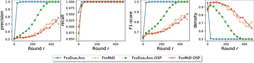
Figure 3: Sparsity recovery on a synthetic LASSO problem with 50% sparse ground truth. Observe that FedDualAvg not only identifies most of the sparsity pattern but also is fastest. It is also worth noting that the less-principled FedDualAvg-OSP is also very competitive. The poor performance of FedMiD can be attributed to the “curse of primal averaging”, as the server averaging step “smooths out” the sparsity pattern, which is corroborated empirically by the least sparse solution obtained by FedMiD.

5.2 Federated Low-Rank Matrix Estimation via Nuclear-Norm Regularization

In this subsection, we consider a low-rank matrix estimation problem via the nuclear-norm regularization

$$\min_{W\in\mathbb{R}^{d_{1}\times d_{2}},b\in\mathbb{R}}\frac{1}{M}\sum_{m=1}^{M}\mathbb{E}_{(X,y)\sim\mathcal{D}_{m}}\left(\langle X,W\rangle+b-y\right)^{2}+\lambda\|W\|_{\mathrm{nuc}},$$ (5.2)

where $\|W\|_{\mathrm{nuc}}$ denotes the matrix nuclear norm. The goal is to recover a low-rank matrix $W$ from noisy observations $(X,y)$. This formulation captures a variety of problems such as low-rank matrix completion and recommendation systems (Candès and Recht, 2009). Note that the proximal operator with respect to the nuclear-norm regularizer reduces to singular-value thresholding operation (Cai et al., 2010).

We evaluate the algorithms on a synthetic federated dataset with known low-rank ground truth $W_{\mathrm{real}}\in\mathbb{R}^{d_{1}\times d_{2}}$ and bias $b_{\mathrm{real}}\in\mathbb{R}$, similar to the above LASSO experiments. We focus on four metrics for this task: the training (regularized) loss, the validation mean-squared-error, the recovered rank, and the recovery error in Frobenius norm $\|W_{\mathrm{output}}-W_{\mathrm{real}}\|_{\mathrm{F}}$. We tune the client learning rate $\eta_{\mathrm{c}}$ and server learning rate $\eta_{\mathrm{s}}$ only to attain the best recovery error. We also record the results obtained by the deterministic solver on centralized data, marked as optimum. The results are presented in Fig. 4. We provide the rest of the setup details and more experiments in Section A.3.

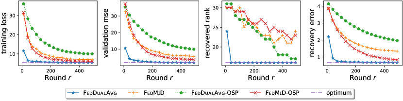
Figure 4: Low-rank matrix estimation comparison on a synthetic dataset with the ground truth of rank 16. We observe that FedDualAvg finds the solution with exact rank in less than 100 communication rounds. FedMiD and FedMiD-OSP converge slower in loss and rank. The unprincipled FedDualAvg-OSP can generate low-rank solutions but is far less accurate.

5.3 Sparse Logistic Regression for fMRI Scan

In this subsection, we consider the cross-silo setup of learning a binary classifier on fMRI scans. For this purpose, we use the data collected by Haxby (2001), to understand the pattern of response in the ventral temporal (vt) area of the brain given a visual stimulus. We plan to learn a sparse ($\ell_{1}$-regularized) binary logistic regression on the voxels to classify the stimuli given the voxels input. Enforcing sparsity is crucial for this task as it allows domain experts to understand which part of the brain is differentiating between the stimuli. We compare the algorithms with two non-federated baselines: 1) centralized corresponds to training on the centralized dataset gathered from all the training clients; 2) local corresponds to training on the local data from only one training client without communication. The results are shown in Fig. 5. In Section A.4.2, we provide another presentation of this experiment to visualize the progress of federated algorithms and understand the robustness to learning rate configurations. The results suggest FedDualAvg not only recovers sparse and accurate solutions, but also behaves most robust to learning-rate configurations. We defer the rest of the setup details to Section A.4.

In Section A.5, we provide another set of experiments on federated constrained optimization for Federated EMNIST dataset (Caldas et al., 2019).

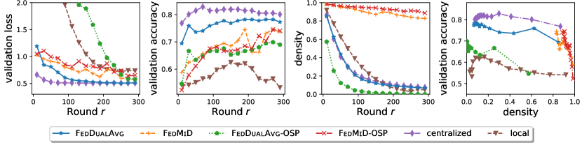
Figure 5: Results on $\ell_{1}$-regularized logistic regression for fMRI data from (Haxby, 2001). We observe that FedDualAvg yields sparse and accurate solutions that are comparable with the centralized baseline. FedMiD and FedMiD-OSP provides denser solutions that are relatively less accurate. The unprincipled FedDualAvg-OSP can provide sparse solutions but far less accurate.

6 Conclusion

In this paper, we have shown the shortcomings of primal FL algorithms for FCO and proposed a primal-dual method (FedDualAvg) to tackle them. Our theoretical and empirical analysis provide strong evidence to support the superior performance of FedDualAvg over natural baselines. Potential future directions include control variates and acceleration based methods for FCO, and applying FCO to personalized settings.

The appendices are structured as follows. In Appendix A, we include additional experiments and detailed setups. In Appendix B, we provide the necessary backgrounds for our theoretical results. We prove two of our main results, namely Theorems 4.2 and 4.3, in Appendices C and D, respectively. The proof of Theorem 4.1 is sketched in Appendix E.

Appendix A Additional Experiments and Setup Details

A.1 General Setup

Algorithms.

In this paper we mainly test four Federated algorithms, namely Federated Mirror Descent (FedMiD, see Algorithm 2), Federated Dual Averaging (FedDualAvg, see Algorithm 3), as well as two less-principled algorithms which skip the client-side proximal operations. We refer to these two algorithms as FedMiD-OSP and FedDualAvg-OSP, where “OSP” stands for ”only server proximal”. We formally state these two OSP algorithms in Algorithms 4 and 5. We study these two OSP algorithms mainly for ablation study purpose, thouse they might be of special interest if the proximal step is computationally intensive. For instance, in FedMiD-OSP, the client proximal step is replaced by $w_{r,k+1}^{m}\leftarrow\nabla h^{*}(\nabla h(w_{r,k}^{m})-\eta_{\mathrm{c}}g_{r,k}^{m})$ with no $\psi$ involved (see line 8 of Algorithm 4). This step reduces to the ordinary SGD $w_{r,k+1}^{m}\leftarrow w_{r,k}^{m}-\eta_{\mathrm{c}}g_{r,k}^{m}$ if $h(w)=\frac{1}{2}\|w\|_{2}^{2}$ in which case both $\nabla h$ and $\nabla h^{*}$ are identity mapping. Theoretically, it is not hard to establish similar rates of Theorem 4.1 for FedMiD-OSP with finite $\psi$. For infinite $\psi$, we need extension of $f$ outside $\textbf{dom}\psi$ to fix regularity. To keep this paper focused, we will not establish these results formally. There is no theoretical guarantee on the convergence of FedDualAvg-OSP.

Algorithm 4 Federated Mirror Descent Only Server Proximal (FedMiD-OSP)

1:  procedure FedMiD-OSP ($w_{0},\eta_{\mathrm{c}},\eta_{\mathrm{s}}$)

2:  for $r=0,\ldots,R-1$ do

3:    sample a subset of clients $\mathcal{S}_{r}\subseteq[M]$

4:    on client for $m\in\mathcal{S}_{r}$ in parallel do

5:      client initialization $w_{r,0}^{m}\leftarrow w_{r}$ $\vartriangleright$ Broadcast primal initialization for round $r$

6:      for $k=0,\ldots,K-1$ do

7:         $g_{r,k}^{m}\leftarrow\nabla f(w_{r,k}^{m};\xi_{r,k}^{m})$ $\vartriangleright$ Query gradient

8:         $w_{r,k+1}^{m}\leftarrow\nabla h^{*}(\nabla h(w_{r,k}^{m})-\eta_{\mathrm{c}}g_{r,k}^{m}$) $\vartriangleright$ Client (primal) update – proximal operation skipped

9:    $\Delta_{r}=\frac{1}{|\mathcal{S}_{r}|}\sum_{m\in\mathcal{S}_{r}}(w_{r,K}^{m}-w_{r,0}^{m})$ $\vartriangleright$ Compute pseudo-anti-gradient

10:    $w_{r+1}\leftarrow\nabla(h+\eta_{\mathrm{s}}\eta_{\mathrm{c}}K\psi)^{*}(\nabla h(w_{r})+\eta_{\mathrm{s}}\Delta_{r})$ $\vartriangleright$ Server (primal) update

Algorithm 5 Federated Dual Averaging Only Server Proximal (FedDualAvg-OSP)

1:  procedure FedDualAvg-OSP($w_{0},\eta_{\mathrm{c}},\eta_{\mathrm{s}}$)

2:  server initialization $z_{0}\leftarrow\nabla h(w_{0})$

3:  for $r=0,\ldots,R-1$ do

4:    sample a subset of clients $\mathcal{S}_{r}\subseteq[M]$

5:    on client for $m\in\mathcal{S}_{r}$ in parallel do

6:      client initialization $z_{r,0}^{m}\leftarrow z_{r}$ $\vartriangleright$ Broadcast dual initialization for round $r$

7:      for $k=0,\ldots,K-1$ do

8:         $w_{r,k}^{m}\leftarrow\nabla h^{*}(z_{r,k}^{m})$ $\vartriangleright$ Compute primal point $w_{r,k}^{m}$ – proximal operation skipped

9:         $g_{r,k}^{m}\leftarrow\nabla f(w_{r,k}^{m};\xi_{r,k}^{m})$ $\vartriangleright$ Query gradient

10:         $z_{r,k+1}^{m}\leftarrow z_{r,k}^{m}-\eta_{\mathrm{c}}g_{r,k}^{m}$ $\vartriangleright$ Client (dual) update

11:    $\Delta_{r}=\frac{1}{|\mathcal{S}_{r}|}\sum_{m\in\mathcal{S}_{r}}(z_{r,K}^{m}-z_{r,0}^{m})$ $\vartriangleright$ Compute pseudo-anti-gradient

12:    $z_{r+1}\leftarrow z_{r}+\eta_{\mathrm{s}}\Delta_{r}$ $\vartriangleright$ Server (dual) update

13:    $w_{r+1}\leftarrow\nabla(h+\eta_{\mathrm{s}}\eta_{\mathrm{c}}(r+1)K\psi)^{*}(z_{r+1})$ $\vartriangleright$ (Optional) Compute server primal state

Environments.

We simulate the algorithms in the TensorFlow Federated (TFF) framework (Ingerman and Ostrowski, 2019). The implementation is based on the Federated Research repository.

Tasks.

We experiment the following four tasks in this work.

1. Federated Lasso ($\ell_{1}$-regularized least squares) for sparse feature selection, see Section A.2.

2. Federated low-rank matrix recovery via nuclear-norm regularization, see Section A.3.

3. Federated sparse ($\ell_{1}$-regularized) logistic regression for fMRI dataset (Haxby, 2001), see Section A.4.

4. Federated constrained optimization for Federated EMNIST dataset (Caldas et al., 2019), see Section A.5.

We take the distance-generating function $h$ to be $h(w):=\frac{1}{2}\|w\|_{2}^{2}$ for all the four tasks. The detailed setups of each experiment are stated in the corresponding subsections.

A.2 Federated LASSO for Sparse Feature Selection

A.2.1 Setup Details

In this experiment, we consider the federated LASSO ($\ell_{1}$-regularized least squares) on a synthetic dataset inspired by models from biomedical and signal processing literature (e.g., Ryali et al. 2010; Chen et al. 2012)

$$\min_{w,b}\quad\frac{1}{M}\sum_{m=1}^{M}\operatorname{\mathbb{E}}_{(x,y)\sim\mathcal{D}_{m}}(x^{\top}w+b-y)_{2}^{2}+\lambda\|w\|_{1}.$$ (A.1)

The goal is to retrieve sparse features of $w$ from noisy observations.

Synthetic Dataset Descriptions.

We first generate the ground truth $w_{\mathrm{real}}$ with $d_{1}$ ones and $d_{0}$ zeros for some $d_{1}+d_{0}=d$, namely

$$w_{\mathrm{real}}=\begin{bmatrix}\textbf{1}_{d_{1}}\\ \textbf{0}_{d_{0}}\end{bmatrix}\in\mathbb{R}^{d},$$ (A.2)

and ground truth $b_{\mathrm{real}}\sim\mathcal{N}(0,1)$.

The observations $(x,y)$ are generated as follows to simulate the heterogeneity among clients. Let $(x_{m}^{(i)},y_{m}^{(i)})$ denotes the $i$-th observation of the $m$-th client. For each client $m$, we first generate and fix the mean $\mu_{m}\sim\mathcal{N}(0,I_{d\times d})$. Then we sample $n_{m}$ pairs of observations following

$$x_{m}^{(i)}=\mu_{m}+\delta_{m}^{(i)},\quad \delta_{m}^{(i)}\sim\mathcal{N}(\mathbf{0}_{d},I_{d\times d}) i=1,\ldots,n_{m}$$ where are i.i.d., for ; (A.3)

$$y_{m}^{(i)}=w_{\mathrm{real}}^{\top}x_{m}^{(i)}+b_{\mathrm{real}}+\varepsilon_{m}^{(i)},\quad \text{where $\varepsilon_{m}^{(i)}\sim\mathcal{N}(0,1)$ are i.i.d., for $i=1,\ldots,n_{m}$}.$$ (A.4)

We test four configurations of the above synthetic dataset.

1. The ground truth $w_{\mathrm{real}}$ has $d_{1}=512$ ones and $d_{0}=512$ zeros. We generate $M=64$ training clients where each client possesses $128$ pairs of samples. There are 8,192 training samples in total.

2. (sparse ground truth) The ground truth $w_{\mathrm{real}}$ has $d_{1}=64$ ones and $d_{0}=960$ zeros. The rest of the configurations are the same as dataset (I).

3. (sparser ground truth) The ground truth $w_{\mathrm{real}}$ has $d_{1}=8$ ones and $d_{0}=1016$ zeros. The rest of the configurations are the same as dataset (I).

4. (more distributed data) The ground truth is the same as (I). We generate $M=256$ training clients where each client possesses $32$ pairs of samples. The total number of training examples are the same.

Evaluation Metrics.

Since the ground truth of the synthetic dataset is known, we can evaluate the quality of the sparse features retrieved by comparing it with the ground truth. To numerically evaluate the sparsity, we treat all the features in $w$ with absolute values smaller than $10^{-2}$ as zero elements, and non-zero otherwise. We evaluate the performance by recording precision, recall, F1-score, and sparse density.

Hyperparameters.

For all algorithms, we tune the client learning rate $\eta_{\mathrm{c}}$ and server learning rate $\eta_{\mathrm{s}}$ only. We test 49 different combinations of $\eta_{\mathrm{c}}$ and $\eta_{\mathrm{s}}$. $\eta_{\mathrm{c}}$ is selected from $\{0.001,0.003,0.01,0.03,0.1,0.3,1\}$, and $\eta_{\mathrm{s}}$ is selected from $\{0.01,0.03,0.1,0.3,1,3,10\}$. All methods are tuned to achieve the best averaged recovery error over the last 100 communication rounds. We claim that the best learning rate combination falls in this range for all the algorithms tested. We draw 10 clients uniformly at random at each communication round and let the selected clients run local algorithms with batch size 10 for one epoch (of its local dataset) for this round. We run 500 rounds in total, though FedDualAvg usually converges to almost perfect solutions in much fewer rounds.

The Fig. 4 presented in the main paper (Section 5.1) is for the synthetic dataset (I). Now we test the performance on the other three datasets.

A.2.2 Results on Synthetic Dataset (II) and (III) with Sparser Ground Truth

We repeat the experiments on the dataset (II) and (III) with $1/2^{4}$ and $1/{2^{7}}$ ground truth density, respectively. The results are shown in Figs. 6 and 7. We observe that FedDualAvg converges to the perfect F1-score in less than 100 rounds, which outperforms the other baselines by a margin. The F1-score of FedDualAvg-OSP converges faster on these sparser datasets than (I), which makes it comparably more competitive. The convergence of FedMiD and FedMiD-OSP remains slow.

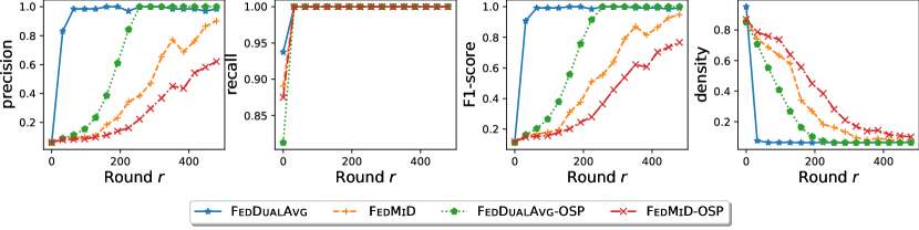
Figure 6: Results on Dataset (II): $1/2^{4}$ Ground Truth Density. See Section A.2.2 for discussions.

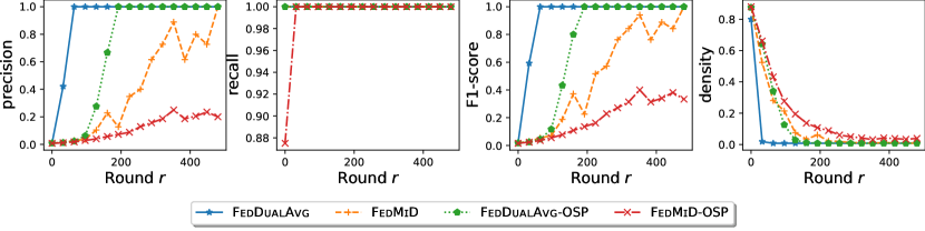
Figure 7: Results on Dataset (III): $1/2^{7}$ Ground Truth Density. See Section A.2.2 for discussions.

A.2.3 Results on Synthetic Dataset (IV): More Distributed Data (256 clients)

We repeat the experiments on the dataset (IV) with more distributed data (256 clients). The results are shown in Fig. 8. We observe that all the four algorithms take more rounds to converge in that each client has fewer data than the previous configurations. FedDualAvg manages to find perfect F1-score in less than 200 rounds, which outperforms the other algorithms significantly. FedDualAvg-OSP can recover an almost perfect F1-score after 500 rounds, but is much slower than on the less distributed dataset (I). FedMiD and FedMiD-OSP have very limited progress within 500 rounds. This is because the server averaging step in FedMiD and FedMiD-OSP fails to aggregate the sparsity patterns properly. Since each client is subject to larger noise due to the limited amount of local data, simply averaging the primal updates will “smooth out” the sparsity pattern.

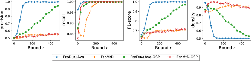
Figure 8: Results on Dataset (IV): More Distributed Data. See Section A.2.3 for discussions.

A.3 Nuclear-Norm-Regularization for Low-Rank Matrix Estimation

A.3.1 Setup Details

In this subsection, we consider a low-rank matrix estimation problem via the nuclear-norm regularization

$$\min_{W\in\mathbb{R}^{d_{1}\times d_{2}},b\in\mathbb{R}}\frac{1}{M}\sum_{m=1}^{M}\mathbb{E}_{(X,y)\sim\mathcal{D}_{m}}\left(\langle X,W\rangle+b-y\right)^{2}+\lambda\|W\|_{\mathrm{nuc}},$$ (A.5)

where $\|W\|_{\mathrm{nuc}}:=\sum_{i}\sigma_{i}(W)$ denotes the nuclear norm (a.k.a. trace norm) defined by the summation of all the singular values. The goal is to recover a low-rank matrix $W$ from noisy observations $(X,y)$. This formulation captures a variety of problems, such as low-rank matrix completion and recommendation systems (c.f. Candès and Recht 2009). Note that the proximal operator with respect to the nuclear-norm regularizer $\|\cdot\|_{\mathrm{nuc}}$ reduces to the well-known singular-value thresholding operation (Cai et al., 2010).

Synthetic Dataset Descriptions.

We first generate the following ground truth $W_{\mathrm{real}}\in\mathbb{R}^{d\times d}$ of rank $r$

$$W_{\mathrm{real}}=\begin{bmatrix}I_{r\times r}&\mathbf{0}_{r\times(d-r)}\\ \mathbf{0}_{(d-r)\times r}&\mathbf{0}_{(d-r)\times(d-r)}\end{bmatrix},$$ (A.6)

and ground truth $b_{\mathrm{real}}\sim\mathcal{N}(0,1)$.

The observations $(X,y)$ are generated as follows to simulate the heterogeneity among clients. Let $(X_{m}^{(i)},y_{m}^{(i)})$ denotes the $i$-th observation of the $m$-th client. For each client $m$, we first generate and fix the mean $\mu_{m}\in\mathbb{R}^{d\times d}$ where all coordinates are i.i.d. standard Gaussian $\mathcal{N}(0,1)$. Then we sample $n_{m}$ pairs of observations following

$$X_{m}^{(i)}=\mu_{m}+\delta_{m}^{(i)},\text{where $\delta_{m}^{(i)}\in\mathbb{R}^{d\times d}$ is a matrix with all coordinates from standard Gaussian;}$$ (A.7)

$$y_{m}^{(i)}=\langle w_{\mathrm{real}},X_{m}^{(i)}\rangle+b_{\mathrm{real}}+\varepsilon_{m}^{(i)},\text{where $\varepsilon_{m}^{(i)}\sim\mathcal{N}(0,1)$ are i.i.d.}$$ (A.8)

We tested four configurations of the above synthetic dataset.

1. The ground truth $W_{\mathrm{real}}$ is a matrix of dimension $32\times 32$ with rank $r=16$. We generate $M=64$ training clients where each client possesses $128$ pairs of samples. There are 8,192 training samples in total.

2. (rank-4 ground truth) The ground truth $W_{\mathrm{real}}$ has rank $r=4$. The other configurations are the same as the dataset (I).

3. (rank-1 ground truth) The ground truth $W_{\mathrm{real}}$ has rank $r=1$. The other configurations are the same as the dataset (I).

4. (more distributed data) The ground truth is the same as (I). We generate $M=256$ training clients where each client possesses $32$ samples. The total number of training examples remains the same.

Evaluation Metrics.

We focus on four metrics for this task: the training (regularized) loss, the validation mean-squared-error, the recovered rank, and the recovery error in Frobenius norm $\|W_{\mathrm{output}}-W_{\mathrm{real}}\|_{\mathrm{F}}$. To numerically evaluate the rank, we count the number of singular values that are greater than $10^{-2}$.

Hyperparameters.

For all algorithms, we tune the client learning rate $\eta_{\mathrm{c}}$ and server learning rate $\eta_{\mathrm{s}}$ only. We test 49 different combinations of $\eta_{\mathrm{c}}$ and $\eta_{\mathrm{s}}$. $\eta_{\mathrm{c}}$ is selected from $\{0.001,0.003,0.01,0.03,0.1,0.3,1\}$, and $\eta_{\mathrm{s}}$ is selected from $\{0.01,0.03,0.1,0.3,1,3,10\}$. All methods are tuned to achieve the best averaged recovery error on the last 100 communication rounds. We claim that the best learning rate combination falls in this range for all algorithms tested. We draw 10 clients uniformly at random at each communication round and let the selected clients run local algorithms with batch size 10 for one epoch (of its local dataset) for this round. We run 500 rounds in total, though FedDualAvg usually converges to perfect F1-score in much fewer rounds.

The Fig. 4 presented in the main paper (Section 5.2) is for the synthetic dataset (I). Now we test the performance of the algorithms on the other three datasets.

A.3.2 Results on Synthetic Dataset (II) and (III) with Ground Truth of Lower Rank

We repeat the experiments on the dataset (II) and (III) with 4 and 1 ground truth rank, respectively. The results are shown in Figs. 9 and 10. The results are qualitatively reminiscent of the previous experiments on the dataset (I). FedDualAvg can recover the exact rank in less than 100 rounds, which outperforms the other baselines by a margin. FedDualAvg-OSP can recover a low-rank solution but is less accurate. The convergence of FedMiD and FedMiD-OSP remains slow.

A.3.3 Results on Synthetic Dataset (IV): More Distributed Data (256 clients)

We repeat the experiments on the dataset (IV) with more distributed data. The results are shown in Fig. 11. We observe that all four algorithms take more rounds to converge in that each client has fewer data than the previous configurations. The other messages are qualitatively similar to the previous experiments – FedDualAvg manages to find exact rank in less than 200 rounds, which outperforms the other algorithms significantly.

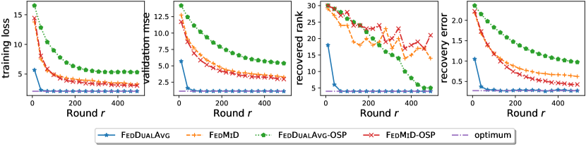
Figure 9: Results on Dataset (II): Ground Truth Rank 4. See Section A.3.2 for discussions.

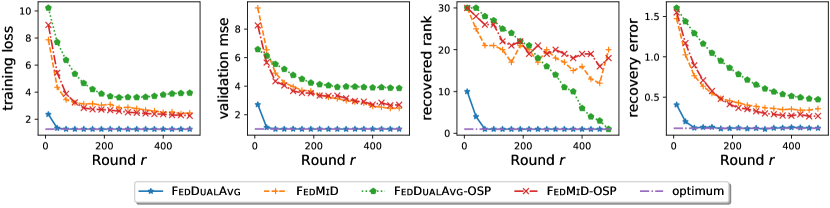
Figure 10: Results on Dataset (III): Ground Truth Rank 1. See Section A.3.2 for discussions.

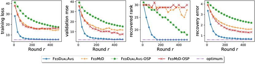
Figure 11: Results on Dataset (IV): More Distributed Data. See Section A.3.3 for discussions.

A.4 Sparse Logistic Regression for fMRI

A.4.1 Setup Details

In this subsection, we provide the additional setup details for the fMRI experiment presented in Fig. 5. The goal is to understand the pattern of response in ventral temporal area of the brain given a visual stimulus. Enforcing sparsity is important as it allows domain experts to understand which part of the brain is differentiating between the stimuli. We apply $\ell_{1}$-regularized logistic regression on the voxels to classify the visual stimuli.

Dataset Descriptions and Preprocessing.

We use data collected by Haxby (2001). There were 6 subjects doing binary image recognition (from a horse and a face) in a block-design experiment over 11-12 sessions per subject, in which each session consists of 18 scans. We use nilearn package (Abraham et al., 2014) to normalize and transform the 4-dimensional raw fMRI scan data into an array with 39,912 volumetric pixels (voxels) using the standard mask. We choose the first 5 subjects as training set and the last subject as validation set. To simulate the cross-silo federated setup, we treat each session as a client. There are 59 training clients and 12 test clients, where each client possesses the voxel data of 18 scans.

Evaluation Metrics.

We focus on three metrics for this task: validation (regularized) loss, validation accuracy, and (sparsity) density. To numerically evaluate the density, we treat all weights with absolute values smaller than $10^{-4}$ as zero elements. The density is computed as non-zero parameters divided by the total number of parameters.

Hyperparameters.

For all algorithms, we adjust only client learning rate $\eta_{\mathrm{c}}$ and server learning rate $\eta_{\mathrm{s}}$. For each federated setup, we tested 49 different combinations of $\eta_{\mathrm{c}}$ and $\eta_{\mathrm{s}}$. $\eta_{\mathrm{c}}$ is selected from $\{0.001,0.003,0.01,0.03,0.1,0.3,1\}$, and $\eta_{\mathrm{s}}$ is selected from $\{0.01,0.03,0.1,0.3,1,3,10\}$. We let each client run its local algorithm with batch-size one for one epoch per round. At the beginning of each round, we draw 20 clients uniformly at random. We run each configuration for 300 rounds and present the configuration with the lowest validation (regularized) loss at the last round.

We also tested two non-federated baselines for comparison, marked as centralized and local. centralized corresponds to training on the centralized dataset gathered from all the 59 training clients. local corresponds to training on the local data from only one training client without communication. We run proximal gradient descent for these two baselines for 300 epochs. The learning rate is tuned from $\{0.0001,0.0003,0.001,0.003,0.01,0.03,0.1,0.3,1\}$ to attain the best validation loss at the last epoch. The results are presented in Fig. 5.

A.4.2 Progress Visualization across Various Learning Rate Configurations

In this subsection, we present an alternative viewpoint to visualize the progress of federated algorithms and understand the robustness to hyper-parameters. To this end, we run four algorithms for various learning rate configurations (we present all the combinations of learning rates mentioned above such that $\eta_{\mathrm{c}}\eta_{\mathrm{s}}\in[0.003,0.3]$) and record the validation accuracy and (sparsity) density after 10th, 30th, 100th, and 300th round. The results are presented in Fig. 12. Each dot stands for a learning rate configuration (client and server). We can observe that most FedDualAvg configurations reach the upper-left region of the box, which indicates sparse and accurate solutions. FedDualAvg-OSP reaches to the mid-left region of the box, which indicates sparse but less accurate solutions. The majority of FedMiD and FedMiD-OSP lands on the right side region box, which reflects the hardness for FedMiD and FedMiD-OSP to find the sparse solutions.

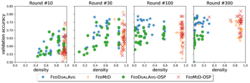
Figure 12: Progress of Federated Algorithms Under Various Learning Rate Configurations for fMRI. Each dot stands for a learning rate configuration (client and server). FedDualAvg recovers sparse and accurate solutions, and is robust to learning-rate configurations.

A.5 Constrained Federated Optimization for Federated EMNIST

A.5.1 Setup Details

In this task we test the performance of the algorithms when the composite term $\psi$ is taken to be convex characteristics $\chi_{\mathcal{C}}(w):=\begin{cases}0&\text{if $w\in\mathcal{C}$},\\ +\infty&\text{if $w\notin\mathcal{C}$}.\end{cases}$ which encodes a hard constraint.

Dataset Descriptions and Models.

We tested on the Federated EMNIST (FEMNIST) dataset provided by TensorFlow Federated, which was derived from the Leaf repository (Caldas et al., 2019). EMNIST is an image classification dataset that extends MNIST dataset by incorporating alphabetical classes. The Federated EMNIST dataset groups the examples from EMNIST by writers.

We tested two versions of FEMNIST in this work:

1. FEMNIST-10: digits-only version of FEMNIST which contains 10 label classes. We experiment the logistic regression models with $\ell_{1}$-ball-constraint or $\ell_{2}$-ball-constraint on this dataset. Note that for this task we only trained on 10% of the examples in the original FEMNIST-10 dataset because the original FEMNIST-10 has an unnecessarily large number (340k) of examples for the logistic regression model.

2. FEMNIST-62: full version of FEMNIST which contains 62 label classes (including 52 alphabetical classes and 10 digital classes). We test a two-hidden-layer fully connected neural network model where all fully connected layers are simultaneously subject to $\ell_{1}$-ball-constraint. Note that there is no theoretical guarantee for either of the four algorithms on non-convex objectives. We directly implement the algorithms as if the objectives were convex. We defer the study of FedMiD and FedDualAvg for non-convex objectives to the future work.

Evaluation Metrics.

We focused on three metrics for this task: training error, training accuracy, and test accuracy. Note that the constraints are always satisfied because all the trajectories of all the four algorithms are always in the feasible region.

Hyperparameters.

For all algorithms, we tune only the client learning rate $\eta_{\mathrm{c}}$ and server learning rate $\eta_{\mathrm{s}}$. For each setup, we tested 25 different combinations of $\eta_{\mathrm{c}}$ and $\eta_{\mathrm{s}}$. $\eta_{\mathrm{c}}$ is selected from $\{0.001,0.003,0.01,0.03,0.1\}$, and $\eta_{\mathrm{s}}$ is selected from $\{0.01,0.03,0.1,0.3,1\}$. We draw 10 clients uniformly at random at each communication round and let the selected clients run local algorithms with batch size 10 for 10 epochs (of its local dataset) for this round. We run 5,000 communication rounds in total and evaluate the training loss every 100 rounds. All methods are tuned to achieve the best averaged training loss on the last 10 checkpoints.

A.5.2 Experimental Results

$\ell_{1}$-Constrained Logistic Regression

We first test the $\ell_{1}$-regularized logistic regression. The results are shown in Fig. 13. We observe that FedDualAvg outperforms the other three algorithms by a margin. Somewhat surprisingly, we observe that the other three algorithms behave very closely in terms of the three metrics tested. This seems to suggest that the client proximal step (in this case projection step) might be saved in FedMiD.

$\ell_{2}$-Constrained Logistic Regression

Next, we test the $\ell_{2}$-regularized logistic regression. The results are shown in Fig. 14. We observe that FedDualAvg outperforms the FedMiD and FedMiD-OSP in all three metrics (note again that FedMiD and FedMiD-OSP share very similar trajectories). Interestingly, the FedDualAvg-OSP behaves much worse in training loss than the other three algorithms, but the training accuracy and validation accuracy are better. We conjecture that this effect might be attributed to the homogeneous property of $\ell_{2}$-constrained logistic regression which FedDualAvg-OSP can benefit from.

$\ell_{1}$-Constrained Two-Hidden-Layer Neural Network

Finally, we test on the two-hidden-layer neural network with $\ell_{1}$-constraints. The results are shown in Fig. 15. We observe that FedDualAvg outperforms FedMiD and FedMiD-OSP in all three metrics (once again, note that FedMiD and FedMiD-OSP share similar trajectories). On the other hand, FedDualAvg-OSP behaves much worse (which is out of the plotting ranges). This is not quite surprising because FedDualAvg-OSP does not have any theoretical guarantees.

Figure 13: $\ell_{1}$-Constrained logistic regression. Dataset: FEMNIST-10. Constraint: $\|w\|_{1}\leq 1000$.

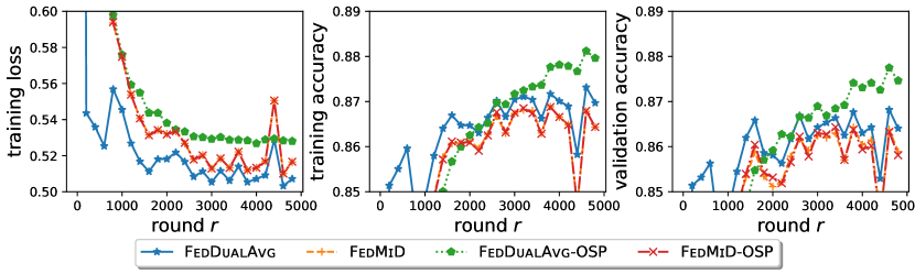
Figure 14: $\ell_{2}$-constrained logistic regression. Dataset: FEMNIST-10. Constraint: $\|w\|_{2}\leq 10$.

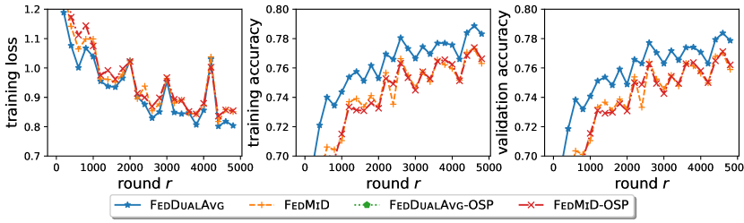
Figure 15: $\ell_{1}$-Constrained Two-Hidden-Layer Neural Network. Dataset: FEMNIST-62. Constraint: all three dense kernels $w^{[l]}$ simultaneously satisfy $\|w^{[l]}\|_{1}\leq 1000$.

Appendix B Theoretical Background and Technicalities

In this section, we introduce some definitions and propositions that are necessary for the proof of our theoretical results. Most of the definitions and results are standard and can be found in the classic convex analysis literature (e.g., Rockafellar 1970; Hiriart-Urruty and Lemaréchal 2001), unless otherwise noted.

The following definition of the effective domain extends the notion of domain (of a finite-valued function) to an extended-valued convex function $\mathbb{R}^{d}\to\mathbb{R}\cup\{+\infty\}$.

Definition B.1 (Effective domain).

Let $g:\mathbb{R}^{d}\to\mathbb{R}\cup\{+\infty\}$ be an extended-valued convex function. The effective domain of $g$, denoted by $\operatorname{\mathbf{dom}}g$, is defined by

$$\operatorname{\mathbf{dom}}g:=\{w\in\mathbb{R}^{d}:g(w)<+\infty\}.$$ (B.1)

In this work we assume all extended-valued convex functions discussed are proper, namely the effective domain is nonempty.

Next, we formally define the concept of strict and strong convexity. Note that the strong convexity is parametrized by some parameter $\mu>0$ and therefore implies strict convexity.

Definition B.2 (Strict and Strong convexity (Hiriart-Urruty and Lemaréchal, 2001, Definition B.1.1.1)).

A convex function $g:\mathbb{R}^{d}\to\mathbb{R}\cup\{+\infty\}$ is strictly convex if for any $w_{1},w_{2}\in\operatorname{\mathbf{dom}}g$, for any $\alpha\in(0,1)$, it is the case that

$$g(\alpha w_{1}+(1-\alpha)w_{2})<\alpha g(w_{1})+(1-\alpha)g(w_{2}).$$ (B.2)

Moreover, $g$ is $\mu$-strongly convex with respect to $\|\cdot\|$ norm if for any $w_{1},w_{2}\in\operatorname{\mathbf{dom}}g$, for any $\alpha\in(0,1)$, it is the case that

$$g(\alpha w_{1}+(1-\alpha)w_{2})\leq\alpha g(w_{1})+(1-\alpha)g(w_{2})-\frac{1}{2}\mu\alpha(1-\alpha)\|w_{2}-w_{1}\|^{2}.$$ (B.3)

The notion of convex conjugate (a.k.a. Legendre-Fenchel transformation) is defined as follows. The outcome of convex conjugate is always convex and closed.

Definition B.3 (Convex conjugate).

Let $g:\mathbb{R}^{d}\to\mathbb{R}\cup\{+\infty\}$ be a convex function. The convex conjugate is defined as

$$g^{*}(z):=\sup_{w\in\mathbb{R}^{d}}\left\{\left\langle z,w\right\rangle-g(w)\right\}.$$ (B.4)

The following result shows that the differentiability of the conjugate function and the strict convexity of the original function is linked.

Proposition B.4 (Differentiability of the conjugate of strictly convex function (Hiriart-Urruty and Lemaréchal, 2001, Theorem E.4.1.1)).

Let $g$: $\mathbb{R}^{d}\to\mathbb{R}\cup\{+\infty\}$ be a closed, strictly convex function. Then we have $\operatorname{\mathbf{int}}\operatorname{\mathbf{dom}}g^{*}\neq\emptyset$ and $g^{*}$ is continuously differentiable on $\operatorname{\mathbf{int}}\operatorname{\mathbf{dom}}g^{*}$ (where $\operatorname{\mathbf{int}}$ stands for interior).

Moreover, for $z\in\operatorname{\mathbf{int}}\operatorname{\mathbf{dom}}g^{*}$, it is the case that

$$\nabla g^{*}(z)=\operatorname*{arg\,min}_{w}\left\{\left\langle-z,w\right\rangle+g(w)\right\}.$$ (B.5)

The differentiability in Eq. B.5 can be strengthened to smoothness if we further assume the strong convexity of the original function $g$.

Proposition B.5 (Smoothness of the conjugate of strongly convex function (Hiriart-Urruty and Lemaréchal, 2001, Theorem E.4.2.1)).

Let $g:\mathbb{R}^{d}\to\mathbb{R}\cup\{+\infty\}$ be a closed, $\mu$-strongly convex function. Then $g^{*}$ is continuously differentiable on $\mathbb{R}^{d}$, and $g^{*}$ is $\frac{1}{\mu}$-smooth on $\mathbb{R}^{d}$, namely $\|\nabla g^{*}(z)-\nabla g^{*}(y)\|^{*}\leq\frac{1}{\mu}\|z-y\|$.

Next we define the Legendre function class.

Definition B.6 (Legendre function (Rockafellar, 1970, §26)).

A proper, convex, closed function $h:\mathbb{R}^{d}\to\mathbb{R}\cup\{+\infty\}$ is of Legendre type if

1. $h$ is strictly convex.

2. $h$ is essentially smooth, namely $h$ is differentiable on $\operatorname{\mathbf{int}}\operatorname{\mathbf{dom}}h$, and $\|\nabla h(w_{k})\|\to\infty$ for every sequence $\{w_{k}\}_{k=0}^{\infty}\subset\operatorname{\mathbf{int}}\operatorname{\mathbf{dom}}h$ converging to a boundary point of $\operatorname{\mathbf{dom}}h$ as $k\to+\infty$.

An important property of the Legendre function is the following proposition (Bauschke et al., 1997).

Proposition B.7 (Rockafellar (1970, Theorem 26.5)).

A convex function $g$ is of Legendre type if and only if its conjugate $g^{*}$ is. In this case, the gradient mapping $\nabla g$ is a toplogical isomorphism with inverse mapping, namely $(\nabla g)^{-1}=\nabla g^{*}$.

Next, recall the definition of Bregman divergence:

Definition B.8 (Bregman divergence (Bregman, 1967)).

Let $g:\mathbb{R}^{d}\to\mathbb{R}\cup\{+\infty\}$ be a closed, strictly convex function that is differentiable in $\operatorname{\mathbf{int}}\operatorname{\mathbf{dom}}g$. The Bregman divergence $D_{g}(w,u)$ for $w\in\operatorname{\mathbf{dom}}g$, $u\in\operatorname{\mathbf{int}}\operatorname{\mathbf{dom}}g$ is defined by

$$D_{g}(w,u)=g(w)-g(u)-\left\langle\nabla g(u),w-u\right\rangle.$$ (B.6)

Note the definition of Bregman divergence requires the differentiability of the base function $g$. To extend the concept of Bregman divergence to non-differentiable function $g$, we consider the following generalized Bregman divergence (slightly modified from (Flammarion and Bach, 2017)). The generalized Bregman divergence plays an important role in the analysis of FedDualAvg.

Definition B.9 (Generalized Bregman divergence (slightly modified from Flammarion and Bach, 2017, Section B.2)).

Let $g:\mathbb{R}^{d}\to\mathbb{R}\cup\{+\infty\}$ be a closed strictly convex function (which may not be differentiable). The Generalized Bregman divergence $\tilde{D}_{g}(w,z)$ for $w\in\operatorname{\mathbf{dom}}g$, $z\in\operatorname{\mathbf{int}}\operatorname{\mathbf{dom}}g^{*}$ is defined by

$$\tilde{D}_{g}(w,u)=g(w)-g(\nabla g^{*}(z))-\left\langle z,w-\nabla g^{*}(z)\right\rangle.$$ (B.7)

Note that $\nabla g^{*}$ is well-defined because $g^{*}$ is differentiable in $\operatorname{\mathbf{int}}\operatorname{\mathbf{dom}}g^{*}$ according to Eq. B.5.

The generalized Bregman divergence is lower bounded by the ordinary Bregman divergence in the following sense.

Proposition B.10 ((Flammarion and Bach, 2017, Lemma 6)).

Let $h:\mathbb{R}^{d}\to\mathbb{R}\cup\{+\infty\}$ be a Legendre function. Let $\psi:\mathbb{R}^{d}\to\mathbb{R}$ be a convex function (which may not be differentiable). Then for any $w\in\operatorname{\mathbf{dom}}h$, for any $z\in\operatorname{\mathbf{int}}\operatorname{\mathbf{dom}}(h+\psi)^{*}$, the following inequality holds

$$\tilde{D}_{h+\psi}(w,z)\geq D_{h}(w,\nabla(h+\psi)^{*}(z)).$$ (B.8)

Proof of Proposition B.10.

The proof is very similar to Lemma 6 of (Flammarion and Bach, 2017), and we include for completeness. By definition of the generalized Bregman divergence (Definition B.9),

$$\tilde{D}_{h+\psi}(w,z)=(h+\psi)(w)-(h+\psi)(\nabla(h+\psi)^{*}(z))-\left\langle z,w-\nabla(h+\psi)^{*}(z)\right\rangle.$$ (B.9)

By definition of the (ordinary) Bregman divergence (Definition B.8),

$$D_{h}(w,\nabla(h+\psi)^{*}(z))=h(w)-h(\nabla(h+\psi)^{*}(z))-\left\langle\nabla h\left(\nabla(h+\psi)^{*}(z)\right),w-\nabla(h+\psi)^{*}(z)\right\rangle.$$ (B.10)

Taking difference,

$$\tilde{D}_{h+\psi}(w,z)-D_{h}(w,\nabla(h+\psi)^{*}(z))=\psi(w)-\psi\left(\nabla(h+\psi)^{*}(z)\right)-\left\langle z-\nabla h\left(\nabla(h+\psi)^{*}(z)\right),w-\nabla(h+\psi)^{*}(z)\right\rangle.$$ (B.11)

By Eq. B.5, one has $z\in\partial(h+\psi)(\nabla(h+\psi)^{*}(z))$. Since $h$ is differentiable in $\operatorname{\mathbf{int}}\operatorname{\mathbf{dom}}h$, we have (by subgradient calculus)

$$z-\nabla h(\nabla(h+\psi)^{*}(z))\in\partial\psi(\nabla(h+\psi)^{*}(z)).$$ (B.12)

Therefore by the property of subgradient as the supporting hyperplane,

$$\psi(w)\geq\psi(\nabla(h+\psi)^{*}(z))+\left\langle z-\nabla h\left(\nabla(h+\psi)^{*}(z)\right),w-\nabla\left(h+\psi\right)^{*}(z)\right\rangle$$ (B.13)

Combining Eq. B.11 and Eq. B.13 yields

$$\tilde{D}_{h+\psi}(w,z)-D_{h}(w,\nabla(h+\psi)^{*}(z))\geq 0,$$ (B.14)

completing the proof. ∎

Appendix C Proof of Theorem 4.2: Convergence of FedDualAvg Under Bounded Gradient Assumption

In this section, we provde a complete, non-asymptotic version of Theorem 4.2 with detailed proof.

We now formally state the assumptions of Theorem 4.2 for ease of reference.

Assumption 3 (Bounded gradient).

In addition to Assumption 1, assume that the gradient is $G$-uniformly-bounded, namely

$$\sup_{w\in\operatorname{\mathbf{dom}}\psi}\|\nabla f(w,\xi)\|_{*}\leq G$$ (C.1)

This is a standard assumption in analyzing classic distributed composite optimization (Duchi et al., 2012).

Before we start, we introduce a few more notations to simplify the exposition and analysis throughout this section. Let $h_{r,k}(w)=h(w)+(rK+k)\eta_{\mathrm{c}}\psi(w)$. Let $\overline{z_{r,k}}:=\frac{1}{M}\sum_{m=1}^{M}z_{r,k}^{m}$ denote the average over clients, and $\widehat{w_{r,k}}:=\nabla h_{r,k}^{*}(\overline{z_{r,k}})$ denote the primal image of $\overline{z_{r,k}}$. Formally, we use $\mathcal{F}_{r,k}$ to denote the $\sigma$-algebra generated by $\{z_{\rho,\kappa}^{m}:\rho<r\text{ or }(\rho=r\text{ and }\kappa\leq k),m\in[M]\}$.

C.1 Main Theorem and Lemmas

Now we introduce the full version of Theorem 4.2 regarding the convergence of FedDualAvg with unit server learning rate $\eta_{\mathrm{s}}=1$ under bounded gradient assumptions.

Theorem C.1 (Detailed version of Theorem 4.2).

Assume Assumption 3, then for any initialization $w_{0}\in\operatorname{\mathbf{dom}}\psi$, for unit server learning rate $\eta_{\mathrm{s}}=1$ and any client learning rate $\eta_{\mathrm{c}}\leq\frac{1}{4L}$, FedDualAvg yields

$$\operatorname{\mathbb{E}}\left[\Phi\left(\frac{1}{KR}\sum_{r=0}^{R-1}\sum_{k=1}^{K}\widehat{w_{r,k}}\right)-\Phi(w^{\star})\right]\leq\frac{B}{\eta_{\mathrm{c}}KR}+\frac{\eta_{\mathrm{c}}\sigma^{2}}{M}+4\eta_{\mathrm{c}}^{2}L(K-1)^{2}G^{2},$$ (C.2)

where $B:=D_{h}(w^{\star},w_{0})$ is the Bregman divergence between the optimal $w^{*}$ and the initial $w_{0}$.

Particularly for

$$\eta_{\mathrm{c}}=\min\left\{\frac{1}{4L},\frac{M^{\frac{1}{2}}B^{\frac{1}{2}}}{\sigma K^{\frac{1}{2}}R^{\frac{1}{2}}},\frac{B^{\frac{1}{3}}}{L^{\frac{1}{3}}KR^{\frac{1}{3}}G^{\frac{2}{3}}}\right\},$$ (C.3)

one has

$$\operatorname{\mathbb{E}}\left[\Phi\left(\frac{1}{KR}\sum_{r=0}^{R-1}\sum_{k=1}^{K}\widehat{w_{r,k}}\right)-\Phi(w^{\star})\right]\leq\frac{4LB}{KR}+\frac{2\sigma B^{\frac{1}{2}}}{M^{\frac{1}{2}}K^{\frac{1}{2}}R^{\frac{1}{2}}}+\frac{5L^{\frac{1}{3}}B^{\frac{2}{3}}G^{\frac{2}{3}}}{R^{\frac{2}{3}}}.$$ (C.4)

The proof of Theorem C.1 is based on the following two lemmas regarding perturbed convergence and stability respectively.

Lemma C.2 (Perturbed iterate analysis of FedDualAvg).

Assume Assumption 1, then for any initialization $w_{0}\in\operatorname{\mathbf{dom}}\psi$, for any reference point $w\in\operatorname{\mathbf{dom}}\psi$, for $\eta_{\mathrm{s}}=1$, for any $\eta_{\mathrm{c}}\leq\frac{1}{4L}$, FedDualAvg yields

$$\operatorname{\mathbb{E}}\left[\Phi\left(\frac{1}{KR}\sum_{r=0}^{R-1}\sum_{k=1}^{K}\widehat{w_{r,k}}\right)-\Phi(w)\right]\leq\frac{1}{\eta_{\mathrm{c}}KR}D_{h}(w,w_{0})+\frac{\eta_{\mathrm{c}}\sigma^{2}}{M}+\frac{L}{MKR}\left[\sum_{r=0}^{R-1}\sum_{k=0}^{K-1}\sum_{m=1}^{M}\operatorname{\mathbb{E}}\left\|\overline{z_{r,k}}-z_{r,k}^{m}\right\|_{*}^{2}\right].$$ (C.5)

Lemma C.2 decomposes the convergence of FedDualAvg into two parts: the first part $\frac{1}{\eta_{\mathrm{c}}KR}D_{h}(w,w_{0})+\frac{\eta_{\mathrm{c}}\sigma^{2}}{2M}+\frac{L}{MKR}$ corresponds to the convergence rate if all clients were synchronized every iteration. The second part $\frac{L}{MKR}\sum_{r=0}^{R-1}\sum_{k=0}^{K-1}\sum_{m=1}^{M}\operatorname{\mathbb{E}}\|z_{r,k}^{m}-\overline{z_{r,k}}\|_{*}^{2}$ characterizes the stability of the algorithm. Note that Lemma C.2 only assumes the blanket Assumption 1. We defer the proof of Lemma C.2 to Section C.2.

The following Lemma C.3 bounds the stability term under the additional bounded gradient assumptions.

Lemma C.3 (Stability of FedDualAvg under bounded gradient assumption).

In the same settings of Theorem C.1, it is the case that

$$\frac{1}{M}\sum_{m=1}^{M}\operatorname{\mathbb{E}}\left\|z_{r,k}^{m}-\overline{z_{r,k}}\right\|_{*}^{2}\leq 4\eta_{\mathrm{c}}^{2}(K-1)^{2}G^{2}.$$ (C.6)

We defer the proof of Lemma C.3 to Section C.3. With Lemmas C.2 and C.3 at hands the proof of Theorem C.1 is immediate.

Proof of Theorem C.1.

Eq. C.2 follows immediately from Lemmas C.2 and C.3 by putting $w=w^{\star}$ in Lemma C.2.

Now put

$$\eta_{\mathrm{c}}=\min\left\{\frac{1}{4L},\frac{M^{\frac{1}{2}}B^{\frac{1}{2}}}{\sigma K^{\frac{1}{2}}R^{\frac{1}{2}}},\frac{B^{\frac{1}{3}}}{L^{\frac{1}{3}}KR^{\frac{1}{3}}G^{\frac{2}{3}}}\right\},$$ (C.7)

which yields

$$\frac{B}{\eta_{\mathrm{c}}KR}=\max\left\{\frac{4LB}{KR},\frac{\sigma B^{\frac{1}{2}}}{M^{\frac{1}{2}}K^{\frac{1}{2}}R^{\frac{1}{2}}},\frac{L^{\frac{1}{3}}B^{\frac{2}{3}}G^{\frac{2}{3}}}{R^{\frac{2}{3}}}\right\}\leq\frac{4LB}{KR}+\frac{\sigma B^{\frac{1}{2}}}{M^{\frac{1}{2}}K^{\frac{1}{2}}R^{\frac{1}{2}}}+\frac{L^{\frac{1}{3}}B^{\frac{2}{3}}G^{\frac{2}{3}}}{R^{\frac{2}{3}}},$$ (C.8)

and

$$\frac{\eta_{\mathrm{c}}\sigma^{2}}{2M}\leq{\frac{M^{\frac{1}{2}}B^{\frac{1}{2}}}{\sigma T^{\frac{1}{2}}}}\cdot\frac{\sigma^{2}}{2M}=\frac{\sigma B^{\frac{1}{2}}}{2M^{\frac{1}{2}}K^{\frac{1}{2}}R^{\frac{1}{2}}},\qquad 4\eta_{\mathrm{c}}^{2}LK^{2}G^{2}\leq 4\left(\frac{B^{\frac{1}{3}}}{L^{\frac{1}{3}}KR^{\frac{1}{3}}G^{\frac{2}{3}}}\right)^{2}LK^{2}G^{2}=\frac{4L^{\frac{1}{3}}B^{\frac{2}{3}}G^{\frac{2}{3}}}{R^{\frac{2}{3}}}.$$ (C.9)

Summarizing the above three inequalities completes the proof of Theorem C.1. ∎

C.2 Perturbed Iterate Analysis of FedDualAvg: Proof of Lemma C.2

In this subsection, we prove Lemma C.2. We start by showing the following Proposition C.4 regarding the one step improvement of the shadow sequence $\overline{z_{r,k}}$.

Proposition C.4 (One step analysis of FedDualAvg).

Under the same assumptions of Lemma C.2, the following inequality holds

$$\operatorname{\mathbb{E}}\left[\tilde{D}_{h_{r,k+1}}(w,\overline{z_{r,k+1}})\middle|\mathcal{F}_{r,k}\right]\leq \tilde{D}_{h_{r,k}}(w,\overline{z_{r,k}})-\eta_{\mathrm{c}}\operatorname{\mathbb{E}}\left[\Phi(\widehat{w_{r,k+1}})-\Phi(w)\middle|\mathcal{F}_{r,k}\right]$$ (C.10)

$$+\eta_{\mathrm{c}}L\cdot\operatorname{\mathbb{E}}\left[\frac{1}{M}\sum_{m=1}^{M}\left\|\overline{z_{r,k}}-z_{r,k}^{m}\right\|_{*}^{2}\middle|\mathcal{F}_{r,k}\right]+\frac{\eta_{\mathrm{c}}^{2}\sigma^{2}}{M},$$ (C.11)

where $\tilde{D}$ is the generalized Bregman divergence defined in Definition B.9.

The proof of Proposition C.4 relies on the following two claims regarding the deterministic analysis of FedDualAvg. We defer the proof of Claims C.5 and C.6 to Sections C.2.1 and C.2.2, respectively.

Claim C.5.

Under the same assumptions of Lemma C.2, the following inequality holds

$$\tilde{D}_{h_{r,k+1}}(w,\overline{z_{r,k+1}})$$ (C.12)

$$= \tilde{D}_{h_{r,k}}(w,\overline{z_{r,k}})-\tilde{D}_{h_{r,k}}(\widehat{w_{r,k+1}},\overline{z_{r,k}})-\eta_{\mathrm{c}}(\psi(\widehat{w_{r,k+1}})-\psi(w)))-\eta_{\mathrm{c}}\left\langle\frac{1}{M}\sum_{m=1}^{M}\nabla f(w_{r,k}^{m};\xi_{r,k}^{m}),\widehat{w_{r,k+1}}-w\right\rangle.$$ (C.13)

Claim C.6.

Under the same assumptions of Lemma C.2, it is the case that

$$F(\widehat{w_{r,k+1}})-F(w)\leq\left\langle\frac{1}{M}\sum_{m=1}^{M}\nabla f(w_{r,k}^{m};\xi_{r,k}^{m}),\widehat{w_{r,k+1}}-w\right\rangle$$ (C.14)

$$\qquad\qquad+\left\langle\frac{1}{M}\sum_{m=1}^{M}\left(\nabla F_{m}(w_{r,k}^{m})-\nabla f(w_{r,k}^{m};\xi_{r,k}^{m})\right),\widehat{w_{r,k+1}}-w\right\rangle+L\|\widehat{w_{r,k+1}}-\widehat{w_{r,k}}\|^{2}+\frac{L}{M}\sum_{m=1}^{M}\left\|\overline{z_{r,k}}-z_{r,k}^{m}\right\|_{*}^{2}.$$ (C.15)

With Claims C.5 and C.6 at hand we are ready to prove the one step analysis Proposition C.4.

Proof of Proposition C.4.

Applying Claims C.5 and C.6 yields (summating Eq. C.13 with $\eta_{c}$ times of Eq. C.15),

$$\tilde{D}_{h_{r,k+1}}(w,\overline{z_{r,k+1}})\leq \tilde{D}_{h_{r,k}}(w,\overline{z_{r,k}})-\tilde{D}_{h_{r,k}}(\widehat{w_{r,k+1}},\overline{z_{r,k}})+\eta_{\mathrm{c}}L\|\widehat{w_{r,k+1}}-\widehat{w_{r,k}}\|^{2}-\eta_{\mathrm{c}}\left(\Phi(\widehat{w_{r,k+1}})-\Phi(w)\right)$$ (C.16)

$$+\eta_{\mathrm{c}}\left\langle\frac{1}{M}\sum_{m=1}^{M}\left(\nabla F_{m}(w_{r,k}^{m})-\nabla f(w_{r,k}^{m};\xi_{r,k}^{m})\right),\widehat{w_{r,k+1}}-w\right\rangle$$ (C.17)

$$+\eta_{\mathrm{c}}L\cdot\frac{1}{M}\sum_{m=1}^{M}\left\|\overline{z_{r,k}}-z_{r,k}^{m}\right\|_{*}^{2}.$$ (C.18)

Note that

$$\tilde{D}_{h_{r,k}}(\widehat{w_{r,k+1}},\overline{z_{r,k}})\geq D_{h}(\widehat{w_{r,k+1}},\nabla h_{r,k}^{*}(\overline{z_{r,k}}))=D_{h}(\widehat{w_{r,k+1}},\widehat{w_{r,k}})\geq\frac{1}{2}\|\widehat{w_{r,k+1}}-\widehat{w_{r,k}}\|^{2},$$ (C.19)

and

$$\eta_{\mathrm{c}}L\|\widehat{w_{r,k+1}}-\widehat{w_{r,k}}\|^{2}\leq\frac{1}{4}\|\widehat{w_{r,k+1}}-\widehat{w_{r,k}}\|^{2},$$ (C.20)

since $\eta_{\mathrm{c}}\leq\frac{1}{4L}$ by assumption. Therefore,

$$-\tilde{D}_{h_{r,k}}(\widehat{w_{r,k+1}},\overline{z_{r,k}})+\eta_{\mathrm{c}}L\|\widehat{w_{r,k+1}}-\widehat{w_{r,k}}\|^{2}\leq-\frac{1}{4}\|\widehat{w_{r,k+1}}-\widehat{w_{r,k}}\|^{2}.$$ (C.21)

Plugging Eq. C.21 to Eq. C.18 gives

$$\tilde{D}_{h_{r,k+1}}(w,\overline{z_{r,k+1}})\leq \tilde{D}_{h_{r,k}}(w,\overline{z_{r,k}})-\frac{1}{4}\|\widehat{w_{r,k+1}}-\widehat{w_{r,k}}\|^{2}-\eta_{\mathrm{c}}\left(\Phi(\widehat{w_{r,k+1}})-\Phi(w)\right)$$ (C.22)

$$+\eta_{\mathrm{c}}\left\langle\frac{1}{M}\sum_{m=1}^{M}\left(\nabla F_{m}(w_{r,k}^{m})-\nabla f(w_{r,k}^{m};\xi_{r,k}^{m})\right),\widehat{w_{r,k+1}}-w\right\rangle$$ (C.23)

$$+\eta_{\mathrm{c}}L\cdot\frac{1}{M}\sum_{m=1}^{M}\left\|\overline{z_{r,k}}-z_{r,k}^{m}\right\|_{*}^{2}.$$ (C.24)

Now we take conditional expectation. Note that

$$\operatorname{\mathbb{E}}\left[\left\langle\frac{1}{M}\sum_{m=1}^{M}\nabla F_{m}(w_{r,k}^{m})-\nabla f(w_{r,k}^{m};\xi_{r,k}^{m}),\widehat{w_{r,k+1}}-w\right\rangle\middle|\mathcal{F}_{r,k}\right]$$ (C.25)

$$= \operatorname{\mathbb{E}}\left[\left\langle\frac{1}{M}\sum_{m=1}^{M}\nabla F_{m}(w_{r,k}^{m})-\nabla f(w_{r,k}^{m};\xi_{r,k}^{m}),\widehat{w_{r,k+1}}-\widehat{w_{r,k}}\right\rangle\middle|\mathcal{F}_{r,k}\right] \operatorname{\mathbb{E}}_{\xi_{r,k}^{m}\sim\mathcal{D}_{m}}[\nabla f(w_{r,k}^{m};\xi_{r,k}^{m})]=\nabla F_{m}(w_{r,k}^{m})$$ (since )

$$\leq \operatorname{\mathbb{E}}\left[\left\|\frac{1}{M}\sum_{m=1}^{M}\nabla F_{m}(w_{r,k}^{m})-\nabla f(w_{r,k}^{m};\xi_{r,k}^{m})\right\|_{*}\middle|\mathcal{F}_{r,k}\right]\cdot\operatorname{\mathbb{E}}\left[\left\|\widehat{w_{r,k+1}}-\widehat{w_{r,k}}\right\|\middle|\mathcal{F}_{r,k}\right] \|\cdot\|_{*}$$ (by definition of dual norm )

$$\leq \frac{\sigma}{\sqrt{M}}\operatorname{\mathbb{E}}\left[\left\|\widehat{w_{r,k+1}}-\widehat{w_{r,k}}\right\|\middle|\mathcal{F}_{r,k}\right].$$ (by bounded variance assumption and independence)

Plugging the above inequality to Eq. C.24 gives

$$\operatorname{\mathbb{E}}\left[\tilde{D}_{h_{r,k+1}}(w,\overline{z_{r,k+1}})\middle|\mathcal{F}_{r,k}\right]$$ (C.26)

$$\leq \tilde{D}_{h_{r,k}}(w,\overline{z_{r,k}})-\eta_{\mathrm{c}}\operatorname{\mathbb{E}}\left[\Phi(\widehat{w_{r,k+1}})-\Phi(w)\middle|\mathcal{F}_{r,k}\right]+\eta_{\mathrm{c}}L\cdot\operatorname{\mathbb{E}}\left[\frac{1}{M}\sum_{m=1}^{M}\left\|\overline{z_{r,k}}-z_{r,k}^{m}\right\|_{*}^{2}\middle|\mathcal{F}_{r,k}\right]$$ (C.27)

$$+\frac{\eta_{\mathrm{c}}\sigma}{\sqrt{M}}\operatorname{\mathbb{E}}\left[\left\|\widehat{w_{r,k+1}}-\widehat{w_{r,k}}\right\|\middle|\mathcal{F}_{r,k}\right]-\frac{1}{4}\operatorname{\mathbb{E}}\left[\|\widehat{w_{r,k+1}}-\widehat{w_{r,k}}\|^{2}\middle|\mathcal{F}_{r,k}\right]$$ (C.28)

$$\leq \tilde{D}_{h_{r,k}}(w,\overline{z_{r,k}})-\eta_{\mathrm{c}}\operatorname{\mathbb{E}}\left[\Phi(\widehat{w_{r,k+1}})-\Phi(w)\middle|\mathcal{F}_{r,k}\right]+\eta_{\mathrm{c}}L\cdot\operatorname{\mathbb{E}}\left[\frac{1}{M}\sum_{m=1}^{M}\left\|\overline{z_{r,k}}-z_{r,k}^{m}\right\|_{*}^{2}\middle|\mathcal{F}_{r,k}\right]+\frac{\eta_{\mathrm{c}}^{2}\sigma^{2}}{M},$$ (by quadratic maximum)

completing the proof of Proposition C.4. ∎

The Lemma C.2 then follows by telescoping the one step analysis Proposition C.4.

Proof of Lemma C.2.

Let us first telescope Proposition C.4 within the same round $r$, from $k=0$ to $K$, which gives

$$\operatorname{\mathbb{E}}\left[\tilde{D}_{h_{r,K}}(w,\overline{z_{r,K}})\middle|\mathcal{F}_{r,0}\right]\leq \tilde{D}_{h_{r,0}}(w,\overline{z_{r,0}})-\eta_{\mathrm{c}}\sum_{k=1}^{K}\operatorname{\mathbb{E}}\left[\Phi(\widehat{w_{r,k}})-\Phi(w)\middle|\mathcal{F}_{r,0}\right]$$ (C.29)

$$+\eta_{\mathrm{c}}L\cdot\operatorname{\mathbb{E}}\left[\frac{1}{M}\sum_{k=0}^{K-1}\sum_{m=1}^{M}\left\|\overline{z_{r,k}}-z_{r,k}^{m}\right\|_{*}^{2}\middle|\mathcal{F}_{r,0}\right]+\frac{\eta_{\mathrm{c}}^{2}K\sigma^{2}}{M}.$$ (C.30)

Since server learning rate $\eta_{\mathrm{s}}=1$ we have $\overline{z_{r,K}}=\overline{z_{r+1,0}}$. Therefore we can telescope the round from $r=0$ to $R$, which gives

$$\operatorname{\mathbb{E}}\left[\tilde{D}_{h_{R,0}}(w,\overline{z_{R,0}})\right]\leq \tilde{D}_{h_{0,0}}(w,\overline{z_{0,0}})-\eta_{\mathrm{c}}\sum_{r=0}^{R-1}\sum_{k=1}^{K}\operatorname{\mathbb{E}}\left[\Phi(\widehat{w_{r,k}})-\Phi(w)\right]$$ (C.31)

$$+\eta_{c}L\cdot\operatorname{\mathbb{E}}\left[\frac{1}{M}\sum_{r=0}^{R-1}\sum_{k=0}^{K-1}\sum_{m=1}^{M}\left\|\overline{z_{r,k}}-z_{r,k}^{m}\right\|_{*}^{2}\right]+\frac{\eta_{\mathrm{c}}^{2}KR\sigma^{2}}{M}.$$ (C.32)

Dividing both sides by $\eta_{\mathrm{c}}\cdot KR$ and rearranging

$$\frac{1}{KR}\sum_{r=0}^{R-1}\sum_{k=1}^{K}\operatorname{\mathbb{E}}\left[\Phi(\widehat{w_{r,k}})-\Phi(w)\right]\leq \frac{1}{\eta_{\mathrm{c}}KR}\left(\tilde{D}_{h_{0,0}}(w,\overline{z_{0,0}})-\operatorname{\mathbb{E}}\left[\tilde{D}_{h_{R,0}}(w,\overline{z_{R,0}})\right]\right)$$ (C.33)

$$+L\cdot\operatorname{\mathbb{E}}\left[\frac{1}{MKR}\sum_{r=0}^{R-1}\sum_{k=0}^{K-1}\sum_{m=1}^{M}\left\|\overline{z_{r,k}}-z_{r,k}^{m}\right\|_{*}^{2}\right]+\frac{\eta_{\mathrm{c}}\sigma^{2}}{M}.$$ (C.34)

Applying Jensen’s inequality on the LHS and dropping the negative term on the RHS yield

$$\operatorname{\mathbb{E}}\left[\Phi\left(\frac{1}{KR}\sum_{r=0}^{R-1}\sum_{k=1}^{K}\widehat{w_{r,k}}\right)-\Phi(w)\right]\leq\frac{1}{\eta_{\mathrm{c}}KR}\tilde{D}_{h_{0,0}}(w,\overline{z_{0,0}})+\frac{L}{MKR}\left[\sum_{r=0}^{R-1}\sum_{k=0}^{K-1}\sum_{m=1}^{M}\operatorname{\mathbb{E}}\left\|\overline{z_{r,k}}-z_{r,k}^{m}\right\|_{*}^{2}\right]+\frac{\eta_{\mathrm{c}}\sigma^{2}}{M}.$$ (C.35)

Since $\overline{z_{0,0}}=\nabla h(w_{0})$ and $w_{0}\in\operatorname{\mathbf{dom}}\psi$, we have $\nabla h_{0,0}^{*}(\nabla h(w_{0}))=w_{0}$ by Proposition B.7 since $h$ is assumed to be of Legendre type. Consequently

$$\tilde{D}_{h_{0,0}}(w,\overline{z_{0}}) =h(w)-h(\nabla h_{0,0}^{*}(\nabla h(w_{0})))-\left\langle z_{0},w-\nabla h_{0,0}^{*}(\nabla h(w_{0}))\right\rangle$$ (C.36)

$$=h(w)-h(w_{0})-\left\langle\nabla h(w_{0}),w-w_{0}\right\rangle=D_{h}(w,w_{0}).$$ (C.37)

Plugging Eq. C.37 back to Eq. C.35 completes the proof of Lemma C.2. ∎

C.2.1 Deferred Proof of Claim C.5

Proof of Claim C.5.

By definition of FedDualAvg procedure, for all $m\in[M]$, $k\in\{0,1,\ldots,K-1\}$, we have

$$z_{r,k+1}^{m}=z_{r,k}^{m}-\eta_{\mathrm{c}}\nabla f(w_{r,k}^{m};\xi_{r,k}^{m}).$$ (C.38)

Taking average over $m\in[M]$ gives (recall the overline denotes the average over clients)

$$\overline{z_{r,k+1}}=\overline{z_{r,k}}-\eta_{\mathrm{c}}\cdot\frac{1}{M}\sum_{m=1}^{M}\nabla f(w_{r,k}^{m};\xi_{r,k}^{m}).$$ (C.39)

Now we study generalized Bregman divergence $\tilde{D}_{h,k+1}(w,\overline{z_{r,k+1}})$ for any arbitrary pre-fixed $w\in\operatorname{\mathbf{dom}}h_{r,k}$

$$\tilde{D}_{h_{r,k+1}}(w,\overline{z_{r,k+1}})$$ (C.40)

$$= h_{r,k+1}(w)-h_{r,k+1}\left(\nabla h_{r,k+1}^{*}(\overline{z_{r,k+1}})\right)-\left\langle\overline{z_{r,k+1}},w-\nabla h_{r,k+1}^{*}(\overline{z_{r,k+1}})\right\rangle \tilde{D}$$ (By definition of )

$$= h_{r,k+1}(w)-h_{r,k+1}\left(\widehat{w_{r,k+1}}\right)-\left\langle\overline{z_{r,k+1}},w-\widehat{w_{r,k+1}}\right\rangle \widehat{w_{r,k+1}}$$ (By definition of )

$$= h_{r,k+1}(w)-h_{r,k+1}\left(\widehat{w_{r,k+1}}\right)-\left\langle\overline{z_{r,k}}-\eta_{\mathrm{c}}\cdot\frac{1}{M}\sum_{m=1}^{M}\nabla f(w_{r,k}^{m};\xi_{r,k}^{m}),w-\widehat{w_{r,k+1}}\right\rangle$$ (By Eq. C.39)

$$= (h_{r,k}(w)+\eta_{\mathrm{c}}\psi(w))-(h_{r,k}(\widehat{w_{r,k+1}})+\eta_{\mathrm{c}}\psi(\widehat{w_{r,k+1}}))-\left\langle\overline{z_{r,k}}-\eta_{\mathrm{c}}\cdot\frac{1}{M}\sum_{m=1}^{M}\nabla f(w_{r,k}^{m};\xi_{r,k}^{m}),w-\widehat{w_{r,k+1}}\right\rangle h_{r,k+1}=h_{r,k}+\eta_{\mathrm{c}}\psi h_{r,k+1}$$ (Since by definition of )

$$= \left[h_{r,k}(w)-h_{r,k}(\widehat{w_{r,k}})-\left\langle\overline{z_{r,k}},w-\widehat{w_{r,k}}\right\rangle\right]-\left[h_{r,k}(\widehat{w_{r,k+1}})-h_{r,k}(\widehat{w_{r,k}})-\left\langle\overline{z_{r,k}},\widehat{w_{r,k+1}}-\widehat{w_{r,k}}\right\rangle\right]$$ (C.41)

$$-\eta_{\mathrm{c}}\left(\psi(\widehat{w_{r,k+1}})-\psi(w)\right)-\eta_{\mathrm{c}}\left\langle\frac{1}{M}\sum_{m=1}^{M}\nabla f(w_{r,k}^{m};\xi_{r,k}^{m}),\widehat{w_{r,k+1}}-w\right\rangle$$ (Rearranging)

$$= \tilde{D}_{h_{r,k}}(w,\overline{z_{r,k}})-\tilde{D}_{h_{r,k}}(\widehat{w_{r,k+1}},\overline{z_{r,k}})-\eta_{\mathrm{c}}(\psi(\widehat{w_{r,k+1}})-\psi(w)))-\eta_{\mathrm{c}}\left\langle\frac{1}{M}\sum_{m=1}^{M}\nabla f(w_{r,k}^{m};\xi_{r,k}^{m}),\widehat{w_{r,k+1}}-w\right\rangle,$$ (C.42)

where the last equality is by definition of $\tilde{D}$. ∎

C.2.2 Deferred Proof of Claim C.6

Proof of Claim C.6.

By smoothness and convexity of $F_{m}$, we know

$$F_{m}(\widehat{w_{r,k+1}}) \leq F_{m}(w_{r,k}^{m})+\left\langle\nabla F_{m}(w_{r,k}^{m}),\widehat{w_{r,k+1}}-w_{r,k}^{m}\right\rangle+\frac{L}{2}\|\widehat{w_{r,k+1}}-w_{r,k}^{m}\|^{2}$$ (smoothness)

$$\leq F_{m}(w)+\left\langle\nabla F_{m}(w_{r,k}^{m}),\widehat{w_{r,k+1}}-w\right\rangle+\frac{L}{2}\|\widehat{w_{r,k+1}}-w_{r,k}^{m}\|^{2}.$$ (convexity)

Taking summation over $m$ gives

$$F(\widehat{w_{r,k+1}})-F(w)=\frac{1}{M}\sum_{m=1}^{M}\left(F_{m}(\widehat{w_{r,k+1}})-F_{m}(w)\right)$$ (C.43)

$$\leq \left\langle\frac{1}{M}\sum_{m=1}^{M}\nabla F_{m}(w_{r,k}^{m}),\widehat{w_{r,k+1}}-w\right\rangle+\frac{L}{2M}\sum_{m=1}^{M}\|\widehat{w_{r,k+1}}-w_{r,k}^{m}\|^{2}$$ (C.44)

$$= \left\langle\frac{1}{M}\sum_{m=1}^{M}\nabla f(w_{r,k}^{m};\xi_{r,k}^{m}),\widehat{w_{r,k+1}}-w\right\rangle+\left\langle\frac{1}{M}\sum_{m=1}^{M}\left(\nabla F_{m}(w_{r,k}^{m})-\nabla f(w_{r,k}^{m};\xi_{r,k}^{m})\right),\widehat{w_{r,k+1}}-w\right\rangle$$ (C.45)

$$\qquad\qquad+\frac{L}{2M}\sum_{m=1}^{M}\|\widehat{w_{r,k+1}}-w_{r,k}^{m}\|^{2}$$ (C.46)

$$\leq \left\langle\frac{1}{M}\sum_{m=1}^{M}\nabla f(w_{r,k}^{m};\xi_{r,k}^{m}),\widehat{w_{r,k+1}}-w\right\rangle+\left\langle\frac{1}{M}\sum_{m=1}^{M}\left(\nabla F_{m}(w_{r,k}^{m})-\nabla f(w_{r,k}^{m};\xi_{r,k}^{m})\right),\widehat{w_{r,k+1}}-w\right\rangle$$ (C.47)

$$\qquad\qquad+L\|\widehat{w_{r,k+1}}-\widehat{w_{r,k}}\|^{2}+\frac{L}{M}\sum_{m=1}^{M}\|\widehat{w_{r,k}}-w_{r,k}^{m}\|^{2},$$ (C.48)

where in the last inequality we applied the triangle inequality (for an arbitrary norm $\|\cdot\|$):

$$\|\widehat{w_{r,k+1}}-w_{r,k}^{m}\|^{2}\leq\left(\|\widehat{w_{r,k+1}}-\widehat{w_{r,k}}\|+\|\widehat{w_{r,k}}-w_{r,k}^{m}\|\right)^{2}\leq 2\|\widehat{w_{r,k+1}}-\widehat{w_{r,k}}\|^{2}+2\|\widehat{w_{r,k}}-w_{r,k}^{m}\|^{2}.$$ (C.49)

Since $\psi$ is convex and $h$ is $1$-strongly-convex according to Assumption 1, we know that $h_{r,k}=h+\eta_{\mathrm{c}}(rK+k)\psi$ is also $1$-strongly-convex. Therefore $h_{r,k}^{*}$ is $1$-smooth by Proposition B.5. Consequently,

$$\left\|w_{r,k}^{m}-\widehat{w_{r,k}}\right\|^{2}=\left\|\nabla h_{r,k}^{*}(z_{r,k}^{m})-\nabla h_{r,k}^{*}(\overline{z_{r,k}})\right\|^{2}\leq\left\|z_{r,k}^{m}-\overline{z_{r,k}}\right\|_{*}^{2},$$ (C.50)

where the first equality is by definition of $w_{r,k}^{m}$ and $\widehat{w_{r,k}}$ and the second inequality is by $1$-smoothness. Plugging Eq. C.50 back to Eq. C.48 completes the proof of Claim C.6. ∎

C.3 Stability of FedDualAvg Under Bounded Gradient Assumptions: Proof of Lemma C.3

The proof of Lemma C.3 is straightforward given the assumption of bounded gradient and the fact that $z_{r,0}^{m_{1}}=z_{r,0}^{m_{2}}$ for all $m_{1},m_{2}\in[M]$.

Proof of Lemma C.3.

Let $m_{1},m_{2}\in[M]$ be two arbitrary clients, then

$$\operatorname{\mathbb{E}}\left[\|z_{r,k}^{m_{1}}-z_{r,k}^{m_{2}}\|_{*}^{2}\middle|\mathcal{F}_{r,0}\right] =\eta_{\mathrm{c}}^{2}\operatorname{\mathbb{E}}\left[\left\|\sum_{\kappa=0}^{k-1}\left(\nabla f(w_{r,\kappa}^{m_{1}};\xi_{r,\kappa}^{m_{1}})-\nabla f(w_{r,\kappa}^{m_{2}};\xi_{r,\kappa}^{m_{2}})\right)\right\|_{*}^{2}\middle|\mathcal{F}_{r,0}\right] z_{r,0}^{m_{1}}=z_{r,0}^{m_{2}}$$ (since )

$$\leq\eta_{\mathrm{c}}^{2}\operatorname{\mathbb{E}}\left[\left(\sum_{\kappa={0}}^{k-1}\left\|\nabla f(w_{r,\kappa}^{m_{1}};\xi_{r,\kappa}^{m_{1}})\right\|_{*}+\sum_{\kappa={0}}^{k-1}\left\|\nabla f(w_{r,\kappa}^{m_{2}};\xi_{r,\kappa}^{m_{2}})\right\|_{*}\right)^{2}\middle|\mathcal{F}_{r,0}\right] \|\cdot\|_{*}$$ (triangle inequality of )

$$\leq\eta_{\mathrm{c}}^{2}(2(k-1)G)^{2}=4\eta_{\mathrm{c}}^{2}(K-1)^{2}G^{2}.$$ (C.51)

By convexity of $\|\cdot\|_{*}$,

$$\frac{1}{M}\sum_{m=1}^{M}\operatorname{\mathbb{E}}\left\|z_{r,k}^{m}-\overline{z_{r,k}}\right\|_{*}^{2}\leq\operatorname{\mathbb{E}}\left\|z_{r,k}^{m_{1}}-z_{r,k}^{m_{2}}\right\|_{*}^{2}\leq 4\eta_{\mathrm{c}}^{2}(K-1)^{2}G^{2},$$ (C.52)

completing the proof of Lemma C.3. ∎

Appendix D Proof of Theorem 4.3: Convergence of FedDualAvg Under Bounded Heterogeneity and Quadratic Assumptions

In this section, we study the convergence of FedDualAvg under Assumption 2 (quadraticness) with unit server learning rate $\eta_{\mathrm{s}}=1$. We provide a complete, non-asymptotic version of Theorem 4.3 with detailed proof, which expands the proof sketch in Section 4.3. We will reuse the notations ($\overline{z_{r,k}}$, $\widehat{w_{r,k}}$, etc.) introduced at the beginning of Appendix C.

D.1 Main Theorem and Lemmas

Now we state the full version of Theorem 4.3 on FedDualAvg with unit server learning rate $\eta_{\mathrm{s}}=1$ under quadratic assumptions.

Theorem D.1 (Detailed version of Theorem 4.3).

Assuming Assumption 2, then for any initialization $w_{0}\in\operatorname{\mathbf{dom}}\psi$, for unit server learning rate $\eta_{\mathrm{s}}=1$ and any client learning rate $\eta_{\mathrm{c}}\leq\frac{1}{4L}$, FedDualAvg yields

$$\operatorname{\mathbb{E}}\left[\Phi\left(\frac{1}{KR}\sum_{r=0}^{R-1}\sum_{k=1}^{K}\widehat{w_{r,k}}\right)-\Phi(w^{\star})\right]\leq\frac{B}{\eta_{\mathrm{c}}KR}+\frac{\eta_{\mathrm{c}}\sigma^{2}}{M}+7\eta_{\mathrm{c}}^{2}LK\sigma^{2}+14\eta_{\mathrm{c}}^{2}LK^{2}\zeta^{2},$$ (D.1)

where $B:=D_{h}(w^{\star},w_{0})$ is the Bregman divergence between the optimal $w^{\star}$ and the initialization $w_{0}$.

Particularly for

$$\eta_{\mathrm{c}}=\min\left\{\frac{1}{4L},\frac{M^{\frac{1}{2}}B^{\frac{1}{2}}}{\sigma K^{\frac{1}{2}}R^{\frac{1}{2}}},\frac{B^{\frac{1}{3}}}{L^{\frac{1}{3}}K^{\frac{2}{3}}R^{\frac{1}{3}}\sigma^{\frac{2}{3}}},\frac{B^{\frac{1}{3}}}{L^{\frac{1}{3}}KR^{\frac{1}{3}}\zeta^{\frac{2}{3}}}\right\},$$ (D.2)

we have

$$\operatorname{\mathbb{E}}\left[\Phi\left(\frac{1}{KR}\sum_{r=0}^{R-1}\sum_{k=1}^{K}\widehat{w_{r,k}}\right)-\Phi(w^{\star})\right]\leq\frac{4LB}{KR}+\frac{2\sigma B^{\frac{1}{2}}}{M^{\frac{1}{2}}K^{\frac{1}{2}}R^{\frac{1}{2}}}+\frac{8L^{\frac{1}{3}}B^{\frac{2}{3}}\sigma^{\frac{2}{3}}}{K^{\frac{1}{3}}R^{\frac{2}{3}}}+\frac{15L^{\frac{1}{3}}B^{\frac{2}{3}}\zeta^{\frac{2}{3}}}{R^{\frac{2}{3}}}.$$ (D.3)

The proof of Theorem D.1 relies on the perturbed iterate analysis Lemma C.2 of FedDualAvg and a stability bound for quadratic objectives, as stated below in Lemma D.2. Note that Lemma C.2 only assumes Assumption 1 and therefore applicable to Theorem D.1.

Lemma D.2.

In the same settings of Theorem D.1, the following inequality holds for any $k\in\left\{0,1,\ldots,K\right\}$ and $r\in\left\{0,1,\ldots,R\right\}$,

$$\frac{1}{M}\sum_{m=1}^{M}\operatorname{\mathbb{E}}\left[\left\|\overline{z_{r,k}}-z_{r,k}^{m}\right\|^{2}_{*}\right]\leq 7\eta_{\mathrm{c}}^{2}K\sigma^{2}+14\eta_{\mathrm{c}}^{2}K^{2}\zeta^{2}.$$ (D.4)

The proof of Lemma D.2 is deferred to Section D.2. With Lemma D.2 at hand we are ready to prove Theorem D.1.

Proof of Theorem D.1.

Applying Lemmas C.2 and D.2 one has

$$\operatorname{\mathbb{E}}\left[\Phi\left(\frac{1}{KR}\sum_{r=0}^{R-1}\sum_{k=1}^{K}\widehat{w_{r,k}}\right)-\Phi(w^{\star})\right]$$ (D.5)

$$\leq \frac{1}{\eta_{\mathrm{c}}KR}D_{h}(w^{\star},w_{0})+\frac{\eta_{\mathrm{c}}\sigma^{2}}{M}+\frac{L}{MKR}\left[\sum_{r=0}^{R-1}\sum_{k=0}^{K-1}\sum_{m=1}^{M}\operatorname{\mathbb{E}}\left\|\overline{z_{r,k}}-z_{r,k}^{m}\right\|_{*}^{2}\right]$$ (by Lemma C.2)

$$\leq \frac{1}{\eta_{\mathrm{c}}KR}D_{h}(w^{\star},w_{0})+\frac{\eta_{\mathrm{c}}\sigma^{2}}{M}+L\cdot\left(7\eta_{\mathrm{c}}^{2}K\sigma^{2}+14\eta_{\mathrm{c}}^{2}K^{2}\zeta^{2}\right)$$ (by Lemma D.2)

$$= \frac{B}{\eta_{\mathrm{c}}KR}+\frac{\eta_{\mathrm{c}}\sigma^{2}}{M}+7\eta_{\mathrm{c}}^{2}LK\sigma^{2}+14\eta_{\mathrm{c}}^{2}LK^{2}\zeta^{2},$$ (D.6)

which gives the first inequality in Theorem D.1.

Now set

$$\eta_{\mathrm{c}}=\min\left\{\frac{1}{4L},\frac{M^{\frac{1}{2}}B^{\frac{1}{2}}}{\sigma K^{\frac{1}{2}}R^{\frac{1}{2}}},\frac{B^{\frac{1}{3}}}{L^{\frac{1}{3}}K^{\frac{2}{3}}R^{\frac{1}{3}}\sigma^{\frac{2}{3}}},\frac{B^{\frac{1}{3}}}{L^{\frac{1}{3}}KR^{\frac{1}{3}}\zeta^{\frac{2}{3}}}\right\}.$$ (D.7)

We have

$$\frac{B}{\eta_{\mathrm{c}}KR}\leq\max\left\{\frac{4LB}{KR},\frac{\sigma B^{\frac{1}{2}}}{M^{\frac{1}{2}}K^{\frac{1}{2}}R^{\frac{1}{2}}},\frac{L^{\frac{1}{3}}B^{\frac{2}{3}}\sigma^{\frac{2}{3}}}{K^{\frac{1}{3}}R^{\frac{2}{3}}},\frac{L^{\frac{1}{3}}B^{\frac{2}{3}}\zeta^{\frac{2}{3}}}{R^{\frac{2}{3}}}\right\},$$ (D.8)

and

$$\frac{\eta_{\mathrm{c}}\sigma^{2}}{M}\leq\frac{\sigma B^{\frac{1}{2}}}{M^{\frac{1}{2}}K^{\frac{1}{2}}R^{\frac{1}{2}}},\qquad 7\eta_{\mathrm{c}}^{2}LK\sigma^{2}\leq\frac{7L^{\frac{1}{3}}B^{\frac{2}{3}}\sigma^{\frac{2}{3}}}{K^{\frac{1}{3}}R^{\frac{2}{3}}},\qquad 14\eta_{\mathrm{c}}^{2}LK^{2}\zeta^{2}\leq\frac{14L^{\frac{1}{3}}B^{\frac{2}{3}}\zeta^{\frac{2}{3}}}{R^{\frac{2}{3}}}.$$ (D.9)

Consequently

$$\frac{B}{\eta_{\mathrm{c}}KR}+\frac{\eta_{\mathrm{c}}\sigma^{2}}{M}+7\eta_{\mathrm{c}}^{2}LK\sigma^{2}+14\eta_{\mathrm{c}}^{2}LK^{2}\zeta^{2}\leq\frac{4LB}{KR}+\frac{2\sigma B^{\frac{1}{2}}}{M^{\frac{1}{2}}K^{\frac{1}{2}}R^{\frac{1}{2}}}+\frac{8L^{\frac{1}{3}}B^{\frac{2}{3}}\sigma^{\frac{2}{3}}}{K^{\frac{1}{3}}R^{\frac{2}{3}}}+\frac{15L^{\frac{1}{3}}B^{\frac{2}{3}}\zeta^{\frac{2}{3}}}{R^{\frac{2}{3}}},$$ (D.10)

completing the proof of Theorem D.1. ∎

D.2 Stability of FedDualAvg Under Quadratic Assumptions: Proof of Lemma D.2

In this subsection, we prove Lemma D.2 on the stability of FedDualAvg for quadratic $F$. We first state and prove the following Proposition D.3 on the one-step analysis of stability.

Proposition D.3.

In the same settings of Theorem D.1, let $m_{1},m_{2}\in[M]$ be two arbitrary clients. Then the following inequality holds

$$\operatorname{\mathbb{E}}\left[\left\|z_{r,k+1}^{m_{1}}-z_{r,k+1}^{m_{2}}\right\|_{Q^{-1}}^{2}\middle|\mathcal{F}_{r,k}\right]\leq\left(1+\frac{1}{K}\right)\left\|z_{r,k}^{m_{1}}-z_{r,k}^{m_{2}}\right\|_{Q^{-1}}^{2}+2\left(1+\frac{1}{K}\right)\eta_{\mathrm{c}}^{2}\sigma^{2}\|Q\|_{2}^{-1}+4(1+K)\eta_{\mathrm{c}}^{2}\zeta^{2}\|Q\|_{2}^{-1}.$$ (D.11)

The proof of Proposition D.3 relies on the following three claims. To simplify the exposition we introduce two more notations for this subsection. For any $r,k,m$, let

$$\varepsilon_{r,k}^{m}:=\nabla f(w_{r,k}^{m};\xi_{r,k}^{m})-\nabla F_{m}(w_{r,k}^{m}),\qquad\delta_{r,k}^{m}:=\nabla F_{m}(w_{r,k}^{m})-\nabla F(w_{r,k}^{m}).$$ (D.12)

The following claim upper bounds the growth of $\left\|z_{r,k+1}^{m_{1}}-z_{r,k+1}^{m_{2}}\right\|_{Q^{-1}}^{2}$. The proof of Claim D.4 is deferred to Section D.2.1.

Claim D.4.

In the same settings of Proposition D.3, the following inequality holds

$$\left\|z_{r,k+1}^{m_{1}}-z_{r,k+1}^{m_{2}}\right\|_{Q^{-1}}^{2}\leq \left(1+\frac{1}{K}\right)\left\|z_{r,k}^{m_{1}}-z_{r,k}^{m_{2}}-\eta_{\mathrm{c}}\cdot Q\left(w_{r,k}^{m_{1}}-w_{r,k}^{m_{2}}\right)-\eta_{\mathrm{c}}\left(\varepsilon_{r,k}^{m_{1}}-\varepsilon_{r,k}^{m_{2}}\right)\right\|_{Q^{-1}}^{2}$$ (D.13)

$$+\left(1+K\right)\eta_{\mathrm{c}}^{2}\left\|\delta_{r,k}^{m_{1}}-\delta_{r,k}^{m_{2}}\right\|_{Q^{-1}}^{2}.$$ (D.14)

The next claim upper bounds the growth of the first term in Eq. D.14 in conditional expectation. We extend the stability technique in (Flammarion and Bach, 2017) to bound this term. The proof of Claim D.5 is deferred to Section D.2.2.

Claim D.5.

In the same settings of Proposition D.3, the following inequality holds

$$\operatorname{\mathbb{E}}\left[\left\|z_{r,k}^{m_{1}}-z_{r,k}^{m_{2}}-\eta_{\mathrm{c}}Q\left(w_{r,k}^{m_{1}}-w_{r,k}^{m_{2}}\right)-\eta_{\mathrm{c}}\left(\varepsilon_{r,k}^{m_{1}}-\varepsilon_{r,k}^{m_{2}}\right)\right\|_{Q^{-1}}^{2}\middle|\mathcal{F}_{r,k}\right]\leq\left\|z_{r,k}^{m_{1}}-z_{r,k}^{m_{2}}\right\|_{Q^{-1}}^{2}+2\eta_{\mathrm{c}}^{2}\sigma^{2}\|Q\|_{2}^{-1}.$$ (D.15)

The third claim upper bounds the growth of the second term in Eq. D.14 under conditional expectation. This is a result of the bounded heterogeneity assumption (Assumption 2(c)). The proof of Claim D.6 is deferred to Section D.2.3.

Claim D.6.

In the same settings of Proposition D.3, the following inequality holds

$$\operatorname{\mathbb{E}}\left[\left\|\delta_{r,k}^{m_{1}}-\delta_{r,k}^{m_{2}}\right\|_{Q^{-1}}^{2}\middle|\mathcal{F}_{r,k}\right]\leq 4\|Q\|_{2}^{-1}\zeta^{2}.$$ (D.16)

The proof of the above claims as well as the main lemma require the following helper claim which we also state here. The proof is also deferred to Section D.2.3.

Claim D.7.

In the same settings of Proposition D.3, the dual norm $\|\cdot\|_{*}$ corresponds to the $\|Q\|_{2}\cdot{Q^{-1}}$-norm, namely $\|z\|_{*}=\sqrt{\|Q\|_{2}\cdot z^{\top}Q^{-1}z}$.

The proof of Proposition D.3 is immediate once we have Claims D.4, D.5 and D.6.

Proof of Proposition D.3.

By Claims D.4, D.5 and D.6,

$$\operatorname{\mathbb{E}}\left[\left\|z_{r,k+1}^{m_{1}}-z_{r,k+1}^{m_{2}}\right\|_{Q^{-1}}^{2}\middle|\mathcal{F}_{r,k}\right]$$ (D.17)

$$\leq \left(1+\frac{1}{K}\right)\operatorname{\mathbb{E}}\left[\left\|z_{r,k}^{m_{1}}-z_{r,k}^{m_{2}}-\eta_{\mathrm{c}}Q\left(w_{r,k}^{m_{1}}-w_{r,k}^{m_{2}}\right)-\eta_{\mathrm{c}}\left(\varepsilon_{r,k}^{m_{1}}-\varepsilon_{r,k}^{m_{2}}\right)\right\|_{Q^{-1}}^{2}\middle|\mathcal{F}_{r,k}\right]$$ (D.18)

$$\qquad+\left(1+K\right)\eta_{\mathrm{c}}^{2}\operatorname{\mathbb{E}}\left[\left\|\delta_{r,k}^{m_{1}}-\delta_{r,k}^{m_{2}}\right\|_{Q^{-1}}^{2}\middle|\mathcal{F}_{r,k}\right]$$ (by Claim D.4)

$$\leq \left(1+\frac{1}{K}\right)\left\|z_{r,k}^{m_{1}}-z_{r,k}^{m_{2}}\right\|_{Q^{-1}}^{2}+2\left(1+\frac{1}{K}\right)\eta^{2}\sigma^{2}\|Q\|_{2}^{-1}+4(1+K)\eta_{\mathrm{c}}^{2}\zeta^{2}\|Q\|_{2}^{-1},$$ (by Claims D.5 and D.6)

completing the proof of Proposition D.3. ∎

The main Lemma D.2 then follows by telescoping Proposition D.3.

Proof of Lemma D.2.

Let $m_{1},m_{2}$ be two arbitrary clients. Telescoping Proposition D.3 from $\mathcal{F}_{r,0}$ to $\mathcal{F}_{r,k}$ gives

$$\operatorname{\mathbb{E}}\left[\left\|z_{r,k}^{m_{1}}-z_{r,k}^{m_{2}}\right\|_{Q^{-1}}^{2}\right]$$ (D.19)

$$\leq \frac{\left(1+\frac{1}{K}\right)^{k}-1}{\frac{1}{K}}\left(2\left(1+\frac{1}{K}\right)\eta_{\mathrm{c}}^{2}\sigma^{2}\|Q\|_{2}^{-1}+4(1+K)\eta_{\mathrm{c}}^{2}\zeta^{2}\|Q\|_{2}^{-1}\right)$$ (telescoping of Proposition D.3)

$$\leq (\mathrm{e}-1)K\left(2\left(1+\frac{1}{K}\right)\eta_{\mathrm{c}}^{2}\sigma^{2}\|Q\|_{2}^{-1}+4(1+K)\eta_{\mathrm{c}}^{2}\zeta^{2}\|Q\|_{2}^{-1}\right) (1+\frac{1}{K})^{k}\leq(1+\frac{1}{K})^{K}<\mathrm{e}$$ (since )

$$\leq (\mathrm{e}-1)K\left(4\eta_{\mathrm{c}}^{2}\sigma^{2}\|Q\|_{2}^{-1}+8K\eta_{\mathrm{c}}^{2}\zeta^{2}\|Q\|_{2}^{-1}\right) 1+\frac{1}{K}\leq 2 1+K\leq 2K$$ (since and )

$$\leq 7\eta_{\mathrm{c}}^{2}K\sigma^{2}\|Q\|_{2}^{-1}+14\eta_{\mathrm{c}}^{2}K^{2}\zeta^{2}\|Q\|_{2}^{-1} 4(\mathrm{e}-1)<7 8(\mathrm{e}-1)<14$$ (since and )

By convexity of $\|\cdot\|^{2}_{Q^{-1}}$ and Proposition D.3 one has

$$\frac{1}{M}\sum_{m=1}^{M}\operatorname{\mathbb{E}}\left[\left\|\overline{z_{r,k}}-z_{r,k}^{m}\right\|_{Q^{-1}}^{2}\right]\leq\operatorname{\mathbb{E}}\left[\left\|z_{r,k}^{m_{1}}-z_{r,k}^{m_{2}}\right\|_{Q^{-1}}^{2}\right]\leq 7\eta_{\mathrm{c}}^{2}K\sigma^{2}\|Q\|_{2}^{-1}+14\eta_{\mathrm{c}}^{2}K^{2}\zeta^{2}\|Q\|_{2}^{-1}.$$ (D.20)

Finally, we switch back to $\|\cdot\|_{*}$ norm following Claim D.7

$$\frac{1}{M}\sum_{m=1}^{M}\operatorname{\mathbb{E}}\left[\left\|\overline{z_{r,k}}-z_{r,k}^{m}\right\|_{*}^{2}\right]\leq 7\eta_{\mathrm{c}}^{2}K\sigma^{2}+14\eta_{\mathrm{c}}^{2}K^{2}\zeta^{2},$$ (D.21)

completing the proof of Lemma D.2. ∎

D.2.1 Deferred Proof of Claim D.4

Proof of Claim D.4.

By definition of FedDualAvg procedure one has

$$z_{r,k+1}^{m} =z_{r,k}^{m}-\eta_{\mathrm{c}}\nabla f(w_{r,k}^{m};\xi_{r,k}^{m})$$ (D.22)

$$=z_{r,k}^{m}-\eta_{\mathrm{c}}\nabla F(w_{r,k}^{m})+\eta_{\mathrm{c}}\left(\nabla F_{m}(w_{r,k}^{m})-\nabla F(w_{r,k}^{m})\right)+\eta_{\mathrm{c}}\left(\nabla f(w_{r,k}^{m};\xi_{r,k}^{m})-\nabla F_{m}(w_{r,k}^{m})\right)$$ (D.23)

$$=z_{r,k}^{m}-\eta_{\mathrm{c}}\nabla F(w_{r,k}^{m})-\eta_{\mathrm{c}}\varepsilon_{r,k}^{m}-\eta_{\mathrm{c}}\delta_{r,k}^{m},$$ (D.24)

where the last equality is by definition of $\varepsilon_{r,k}^{m}$ and $\delta_{r,k}^{m}$. Therefore

$$\left\|z_{r,k+1}^{m_{1}}-z_{r,k+1}^{m_{2}}\right\|_{Q^{-1}}^{2}$$ (D.25)

$$= \left\|z_{r,k}^{m_{1}}-z_{r,k}^{m_{2}}-\eta_{\mathrm{c}}Q\left(w_{r,k}^{m_{1}}-w_{r,k}^{m_{2}}\right)-\eta_{\mathrm{c}}\left(\varepsilon_{r,k}^{m_{1}}-\varepsilon_{r,k}^{m_{2}}\right)-\eta_{\mathrm{c}}\left(\delta_{r,k}^{m_{1}}-\delta_{r,k}^{m_{2}}\right)\right\|_{Q^{-1}}^{2}$$ (by Eq. D.24)

$$= \left\|z_{r,k}^{m_{1}}-z_{r,k}^{m_{2}}-\eta_{\mathrm{c}}Q\left(w_{r,k}^{m_{1}}-w_{r,k}^{m_{2}}\right)-\eta_{\mathrm{c}}\left(\varepsilon_{r,k}^{m_{1}}-\varepsilon_{r,k}^{m_{2}}\right)\right\|_{Q^{-1}}^{2}+\eta_{\mathrm{c}}^{2}\left\|\delta_{r,k}^{m_{1}}-\delta_{r,k}^{m_{2}}\right\|_{Q^{-1}}^{2}$$ (D.26)

$$\quad+2\left\langle z_{r,k}^{m_{1}}-z_{r,k}^{m_{2}}-\eta_{\mathrm{c}}Q\left(w_{r,k}^{m_{1}}-w_{r,k}^{m_{2}}\right)-\eta_{\mathrm{c}}\left(\varepsilon_{r,k}^{m_{1}}-\varepsilon_{r,k}^{m_{2}}\right),\eta_{\mathrm{c}}Q^{-1}\left(\delta_{r,k}^{m_{1}}-\delta_{r,k}^{m_{2}}\right)\right\rangle.$$ (D.27)

By Cauchy-Schwartz inequality and AM-GM inequality one has (for any $\gamma>0$)

$$\left\langle z_{r,k}^{m_{1}}-z_{r,k}^{m_{2}}-\eta_{\mathrm{c}}Q\left(w_{r,k}^{m_{1}}-w_{r,k}^{m_{2}}\right)-\eta_{\mathrm{c}}\left(\varepsilon_{r,k}^{m_{1}}-\varepsilon_{r,k}^{m_{2}}\right),\eta_{\mathrm{c}}Q^{-1}\left(\delta_{r,k}^{m_{1}}-\delta_{r,k}^{m_{2}}\right)\right\rangle$$ (D.28)

$$\leq \left\|z_{r,k}^{m_{1}}-z_{r,k}^{m_{2}}-\eta_{\mathrm{c}}Q\left(w_{r,k}^{m_{1}}-w_{r,k}^{m_{2}}\right)-\eta_{\mathrm{c}}\left(\varepsilon_{r,k}^{m_{1}}-\varepsilon_{r,k}^{m_{2}}\right)\right\|_{Q^{-1}}\left\|\eta_{\mathrm{c}}\left(\delta_{r,k}^{m_{1}}-\delta_{r,k}^{m_{2}}\right)\right\|_{Q^{-1}}$$ (Cauchy-Schwarz inequality)

$$\leq \frac{1}{2\gamma}\left\|z_{r,k}^{m_{1}}-z_{r,k}^{m_{2}}-\eta_{\mathrm{c}}Q\left(w_{r,k}^{m_{1}}-w_{r,k}^{m_{2}}\right)-\eta_{\mathrm{c}}\left(\varepsilon_{r,k}^{m_{1}}-\varepsilon_{r,k}^{m_{2}}\right)\right\|^{2}_{Q^{-1}}+\frac{1}{2}\gamma\left\|\eta_{\mathrm{c}}\left(\delta_{r,k}^{m_{1}}-\delta_{r,k}^{m_{2}}\right)\right\|_{Q^{-1}}^{2}.$$ (AM-GM inequality)

$$\leq \frac{1}{2\gamma}\left\|z_{r,k}^{m_{1}}-z_{r,k}^{m_{2}}-\eta_{\mathrm{c}}Q\left(w_{r,k}^{m_{1}}-w_{r,k}^{m_{2}}\right)-\eta_{\mathrm{c}}\left(\varepsilon_{r,k}^{m_{1}}-\varepsilon_{r,k}^{m_{2}}\right)\right\|^{2}_{Q^{-1}}+\frac{1}{2}\gamma\eta_{\mathrm{c}}^{2}\left\|\left(\delta_{r,k}^{m_{1}}-\delta_{r,k}^{m_{2}}\right)\right\|_{Q^{-1}}^{2}.$$ (D.29)

Plugging Eq. D.29 to Eq. D.27 with $\gamma=K$ gives

$$\left\|z_{r,k+1}^{m_{1}}-z_{r,k+1}^{m_{2}}\right\|_{Q^{-1}}^{2}$$ (D.30)

$$\leq \left(1+\frac{1}{K}\right){\left\|z_{r,k}^{m_{1}}-z_{r,k}^{m_{2}}-\eta_{\mathrm{c}}Q\left(w_{r,k}^{m_{1}}-w_{r,k}^{m_{2}}\right)-\eta_{\mathrm{c}}\left(\varepsilon_{r,k}^{m_{1}}-\varepsilon_{r,k}^{m_{2}}\right)\right\|_{Q^{-1}}^{2}}+\left(1+K\right)\eta_{\mathrm{c}}^{2}{\left\|\delta_{r,k}^{m_{1}}-\delta_{r,k}^{m_{2}}\right\|_{Q^{-1}}^{2}},$$ (D.31)

completing the proof of Claim D.4. ∎

D.2.2 Deferred Proof of Claim D.5

The proof technique of this claim is similar to (Flammarion and Bach, 2017, Lemma 8) which we adapt to fit into our settings.

Proof of Claim D.5.

Let us first expand the $\|\cdot\|_{Q^{-1}}^{2}$:

$$\left\|z_{r,k}^{m_{1}}-z_{r,k}^{m_{2}}-\eta_{\mathrm{c}}Q\left(w_{r,k}^{m_{1}}-w_{r,k}^{m_{2}}\right)-\eta_{\mathrm{c}}\left(\varepsilon_{r,k}^{m_{1}}-\varepsilon_{r,k}^{m_{2}}\right)\right\|_{Q^{-1}}^{2}$$ (D.32)

$$= \left\|z_{r,k}^{m_{1}}-z_{r,k}^{m_{2}}\right\|_{Q^{-1}}^{2}+\left\|\eta Q\left(w_{r,k}^{m_{1}}-w_{r,k}^{m_{2}}\right)\right\|_{Q^{-1}}^{2}+\left\|\eta\left(\varepsilon_{r,k}^{m_{1}}-\varepsilon_{r,k}^{m_{2}}\right)\right\|_{Q^{-1}}^{2}+2\left\langle\eta\left(w_{r,k}^{m_{1}}-w_{r,k}^{m_{2}}\right),\eta\left(\varepsilon_{r,k}^{m_{1}}-\varepsilon_{r,k}^{m_{2}}\right)\right\rangle$$ (D.33)

$$\qquad+2\left\langle z_{r,k}^{m_{1}}-z_{r,k}^{m_{2}},-\eta\left(w_{r,k}^{m_{1}}-w_{r,k}^{m_{2}}\right)\right\rangle+2\left\langle z_{r,k}^{m_{1}}-z_{r,k}^{m_{2}},-\eta Q^{-1}\left(\varepsilon_{r,k}^{m_{1}}-\varepsilon_{r,k}^{m_{2}}\right)\right\rangle.$$ (D.34)

Now we take conditional expectation. Note that by bounded variance assumption one has

$$\operatorname{\mathbb{E}}\left[\left\|\eta_{\mathrm{c}}\left(\varepsilon_{r,k}^{m_{1}}-\varepsilon_{r,k}^{m_{2}}\right)\right\|_{Q^{-1}}^{2}\middle|\mathcal{F}_{r,k}\right]=\|Q\|_{2}^{-1}\cdot\operatorname{\mathbb{E}}\left[\left\|\eta_{\mathrm{c}}\left(\varepsilon_{r,k}^{m_{1}}-\varepsilon_{r,k}^{m_{2}}\right)\right\|_{*}^{2}\middle|\mathcal{F}_{r,k}\right]\leq 2\eta_{\mathrm{c}}^{2}\sigma^{2}\|Q\|_{2}^{-1},$$ (D.35)

where in the first equality we applied Claim D.7.

By unbiased and independence assumptions

$$\operatorname{\mathbb{E}}\left[\varepsilon_{r,k}^{m_{1}}-\varepsilon_{r,k}^{m_{2}}\middle|\mathcal{F}_{r,k}\right]=0.$$ (D.36)

Thus

$$\operatorname{\mathbb{E}}\left[\left\|z_{r,k}^{m_{1}}-z_{r,k}^{m_{2}}-\eta_{\mathrm{c}}Q\left(w_{r,k}^{m_{1}}-w_{r,k}^{m_{2}}\right)-\eta_{\mathrm{c}}\left(\varepsilon_{r,k}^{m_{1}}-\varepsilon_{r,k}^{m_{2}}\right)\right\|_{Q^{-1}}^{2}\middle|\mathcal{F}_{r,k}\right]$$ (D.37)

$$\leq \left\|z_{r,k}^{m_{1}}-z_{r,k}^{m_{2}}\right\|_{Q^{-1}}^{2}\underbrace{+\eta_{\mathrm{c}}^{2}\left\|Q\left(w_{r,k}^{m_{1}}-w_{r,k}^{m_{2}}\right)\right\|_{Q^{-1}}^{2}}_{\text{(I)}}\underbrace{-2\eta_{\mathrm{c}}\left\langle z_{r,k}^{m_{1}}-z_{r,k}^{m_{2}},w_{r,k}^{m_{1}}-w_{r,k}^{m_{2}}\right\rangle}_{\text{(II)}}+2\eta_{\mathrm{c}}^{2}\sigma^{2}\|Q\|_{2}^{-1}.$$ (D.38)

Now we analyze (I), (II) in Eq. D.38. First note that

$$\text{(I)}=\eta_{\mathrm{c}}^{2}\left\|Q\left(w_{r,k}^{m_{1}}-w_{r,k}^{m_{2}}\right)\right\|_{Q^{-1}}^{2}$$ (D.39)

$$= \eta_{\mathrm{c}}^{2}\left\langle w_{r,k}^{m_{1}}-w_{r,k}^{m_{2}},Q\left(w_{r,k}^{m_{1}}-w_{r,k}^{m_{2}}\right)\right\rangle \|\cdot\|_{Q^{-1}}^{2}$$ (by definition of )

$$= \eta_{\mathrm{c}}\left\langle w_{r,k}^{m_{1}}-w_{r,k}^{m_{2}},\eta_{\mathrm{c}}\left(\nabla F(w_{r,k}^{m_{1}})-\nabla F(w_{r,k}^{m_{2}})\right)\right\rangle F$$ (since is quadratic)

$$= \eta_{\mathrm{c}}\left\langle w_{r,k}^{m_{1}}-w_{r,k}^{m_{2}},\nabla(\eta_{\mathrm{c}}F-2h)(w_{r,k}^{m_{1}})-\nabla(\eta_{\mathrm{c}}F-2h)(w_{r,k}^{m_{2}})\right\rangle+2\eta_{\mathrm{c}}\left\langle w_{r,k}^{m_{1}}-w_{r,k}^{m_{2}},\nabla h(w_{r,k}^{m_{1}})-\nabla h(w_{r,k}^{m_{2}})\right\rangle$$ (D.40)

By $L$-smoothness of $F_{m}$ (Assumption 1(c)) we know that $F:=\frac{1}{M}\sum_{m=1}^{M}F_{m}$ is also $L$-smooth. Thus $\eta_{\mathrm{c}}F$ is $\frac{1}{4}$-smooth since $\eta_{\mathrm{c}}\leq\frac{1}{4L}$. Thus $\eta_{\mathrm{c}}F-2h$ is concave since $h$ is $1$-strongly convex, which implies

$$\left\langle w_{r,k}^{m_{1}}-w_{r,k}^{m_{2}},\nabla(\eta_{\mathrm{c}}F-2h)(w_{r,k}^{m_{1}})-\nabla(\eta_{\mathrm{c}}F-2h)(w_{r,k}^{m_{2}})\right\rangle\leq 0.$$ (D.41)

We obtain

$$\text{(I)}\leq 2\eta_{\mathrm{c}}\left\langle w_{r,k}^{m_{1}}-w_{r,k}^{m_{2}},\nabla h(w_{r,k}^{m_{1}})-\nabla h(w_{r,k}^{m_{2}})\right\rangle.$$ (D.42)

Now we study (I)+(II) in Eq. D.38:

$$\text{(I) + (II)}=\eta_{\mathrm{c}}^{2}\left\|Q\left(w_{r,k}^{m_{1}}-w_{r,k}^{m_{2}}\right)\right\|_{Q^{-1}}^{2}-2\eta_{\mathrm{c}}\left\langle z_{r,k}^{m_{1}}-z_{r,k}^{m_{2}},w_{r,k}^{m_{1}}-w_{r,k}^{m_{2}}\right\rangle$$ (D.43)

$$\leq 2\eta_{\mathrm{c}}\left\langle w_{r,k}^{m_{1}}-w_{r,k}^{m_{2}},\nabla h(w_{r,k}^{m_{1}})-\nabla h(w_{r,k}^{m_{2}})\right\rangle-2\eta_{\mathrm{c}}\left\langle w_{r,k}^{m_{1}}-w_{r,k}^{m_{2}},z_{r,k}^{m_{1}}-z_{r,k}^{m_{2}}\right\rangle$$ (by inequality Eq. D.42)

$$= -2\eta_{\mathrm{c}}\left\langle w_{r,k}^{m_{1}}-w_{r,k}^{m_{2}},\left(z_{r,k}^{m_{1}}-\nabla h(w_{r,k}^{m_{1}})\right)-\left(z_{r,k}^{m_{2}}-\nabla h(w_{r,k}^{m_{2}})\right)\right\rangle$$ (D.44)

On the other hand, by definition of $w_{r,k}^{m}$ we have

$$w_{r,k}^{m}=\nabla(h+(rK+k)\eta_{\mathrm{c}}\psi)^{*}(z_{r,k}^{m})=\operatorname*{arg\,min}_{w}\left\{\left\langle-z_{r,k}^{m},w\right\rangle+(rK+k)\eta_{\mathrm{c}}\psi(w)+h(w)\right\}.$$ (D.45)

By subdifferential calculus one has

$$z_{r,k}^{m}-\nabla h(w_{r,k}^{m})\in\partial\left[\eta_{c}(rK+k)\psi(w_{r,k}^{m})\right].$$ (D.46)

By monotonicity of subgradients one has

$$\left\langle w_{r,k}^{m_{1}}-w_{r,k}^{m_{2}},\left(z_{r,k}^{m_{1}}-\nabla h(w_{r,k}^{m_{1}})\right)-\left(z_{r,k}^{m_{2}}-\nabla h(w_{r,k}^{m_{2}})\right)\right\rangle\geq 0.$$ (D.47)

Combining Eqs. D.44 and D.47 gives

$$\text{(I) + (II)}\leq 0.$$ (D.48)

Combining Eqs. D.38 and D.48 completes the proof as

$$\operatorname{\mathbb{E}}\left[\left\|z_{r,k}^{m_{1}}-z_{r,k}^{m_{2}}-\eta_{\mathrm{c}}Q\left(w_{r,k}^{m_{1}}-w_{r,k}^{m_{2}}\right)-\eta_{\mathrm{c}}\left(\varepsilon_{r,k}^{m_{1}}-\varepsilon_{r,k}^{m_{2}}\right)\right\|_{Q^{-1}}^{2}\middle|\mathcal{F}_{r,k}\right]\leq\left\|z_{r,k}^{m_{1}}-z_{r,k}^{m_{2}}\right\|_{Q^{-1}}^{2}+2\eta_{\mathrm{c}}^{2}\sigma^{2}\|Q\|_{2}^{-1}.$$ (D.49)

∎

D.2.3 Deferred Proof of Claims D.6 and D.7

Proof of Claim D.6.

By triangle inequality and AM-GM inequality,

$$\operatorname{\mathbb{E}}\left[\left\|\delta_{r,k}^{m_{1}}-\delta_{r,k}^{m_{2}}\right\|_{Q^{-1}}^{2}|\mathcal{F}_{r,k}\right]$$ (D.50)

$$\leq \operatorname{\mathbb{E}}\left[\left(\|\delta_{r,k}^{m_{1}}\|_{Q^{-1}}+\|\delta_{r,k}^{m_{2}}\|_{Q^{-1}}\right)^{2}\middle|\mathcal{F}_{r,k}\right]$$ (triangle inequality)

$$\leq 2\operatorname{\mathbb{E}}\left[\|\delta_{r,k}^{m_{1}}\|_{Q^{-1}}^{2}+\|\delta_{r,k}^{m_{2}}\|_{Q^{-1}}^{2}\middle|\mathcal{F}_{r,k}\right].$$ (AM-GM inequality)

By Claim D.7,

$$\operatorname{\mathbb{E}}\left[\left\|\delta_{r,k}^{m_{1}}-\delta_{r,k}^{m_{2}}\right\|_{Q^{-1}}^{2}\middle|\mathcal{F}_{r,k}\right]\leq 2\|Q\|_{2}^{-1}\operatorname{\mathbb{E}}\left[\|\delta_{r,k}^{m_{1}}\|_{*}^{2}+\|\delta_{r,k}^{m_{2}}\|_{*}^{2}\middle|\mathcal{F}_{r,k}\right]\leq 4\|Q\|_{2}^{-1}\zeta^{2},$$ (D.51)

where the last inequality is due to bounded heterogeneity Assumption 2(c). This completes the proof of Claim D.6. ∎

Proof of Claim D.7.

Since the primal norm $\|\cdot\|$ is $(\|Q\|_{2}^{-1}\cdot Q)$-norm by Assumption 2(b), the dual norm $\|\cdot\|_{*}$ is $\left(\|Q\|_{2}^{-1}\cdot Q\right)^{-1}=\|Q\|_{2}\cdot Q^{-1}$-norm. ∎

Appendix E Proof of Theorem 4.1

In this section, we state and prove Theorem 4.1 on the convergence of FedDualAvg for small client learning rate $\eta_{\mathrm{c}}$. The intuition is that for sufficiently small client learning rate, FedDualAvg is almost as good as stochastic mini-batch with $R$ iterations and batch-size $MK$. The proof technique is very similar to the above sections and (Karimireddy et al., 2020) so we skip a substantial amount of the proof details. We present the proof for FedDualAvg only since the analysis of FedMiD is very similar.

To facilitate the analysis we re-parameterize the hyperparameters by letting $\eta:=\eta_{\mathrm{s}}\eta_{\mathrm{c}}$, and we treat $(\eta,\eta_{\mathrm{c}})$ as independent hyperparameters (rather than $(\eta_{\mathrm{c}},\eta_{\mathrm{s}})$). We use the notation $h_{r,k}:=h+\tilde{\eta}_{r,k}\cdot\psi=h+(\eta rK+\eta_{\mathrm{c}}k)\psi$, $\overline{z_{r,k}}:=\frac{1}{M}\sum_{m=1}^{M}z_{r,k}^{m}$, and $\widehat{w_{r,k}}:=\nabla h_{r,k}^{*}(\overline{z_{r,k}})$. Note that $\widehat{w_{r,0}}=w_{r,0}^{m}$ for all $m\in[M]$ by definition.

E.1 Main Theorem and Lemmas

Now we state the full version of Theorem 4.1 on FedDualAvg with small client learning rate $\eta_{\mathrm{c}}$.

Theorem E.1 (Detailed version of Theorem 4.1).

Assuming Assumption 1, then for any $\eta\in(0,\frac{1}{4KL}]$, for any initialization $w_{0}\in\operatorname{\mathbf{dom}}\psi$, there exists an $\eta_{\mathrm{c}}^{\max}>0$ (which may depend on $\eta$ and $w_{0}$) such that for any $\eta_{\mathrm{c}}\in(0,\eta_{\mathrm{c}}^{\max}]$, FedDualAvg yields

$$\operatorname{\mathbb{E}}\left[\Phi\left(\frac{1}{R}\sum_{r=1}^{R}\widehat{w_{r,0}}\right)-\Phi(w^{\star})\right]\leq\frac{B}{\eta KR}+\frac{3\eta\sigma^{2}}{M},$$ (E.1)

where $B:=D_{h}(w^{\star},w_{0})$ is the Bregman divergence between the optimal $w^{\star}$ and the initialization $w_{0}$.

In particular for

$$\eta=\min\left\{\frac{1}{4KL},\frac{B^{\frac{1}{2}}M^{\frac{1}{2}}}{K^{\frac{1}{2}}R^{\frac{1}{2}}\sigma}\right\},$$ (E.2)

one has

$$\operatorname{\mathbb{E}}\left[\Phi\left(\frac{1}{R}\sum_{r=1}^{R}\widehat{w_{r,0}}\right)-\Phi(w^{\star})\right]\leq\frac{4LB}{R}+\frac{4\sigma B^{\frac{1}{2}}}{M^{\frac{1}{2}}K^{\frac{1}{2}}R^{\frac{1}{2}}}.$$ (E.3)

The proof of Theorem E.1 relies on the following lemmas.

The first Lemma E.2 analyzes $\tilde{D}_{h_{r+1,0}}(w,\overline{z_{r+1,0}})$. The proof of Lemma E.2 is deferred to Section E.2.

Lemma E.2.

Under the same settings of Theorem E.1, the following inequality holds.

$$\tilde{D}_{h_{r+1,0}}(w,\overline{z_{r+1,0}})-\tilde{D}_{h_{r,0}}(w,\overline{z_{r,0}})$$ (E.4)

$$\leq -\tilde{D}_{h_{r,0}}(\widehat{w_{r+1,0}},\overline{z_{r,0}})-\eta K\left(\Phi(\widehat{w_{r+1,0}})-\Phi(w)\right)+\frac{L}{2}\eta K\|\widehat{w_{r+1,0}}-\widehat{w_{r,0}}\|^{2}$$ (E.5)

$$+\eta K\left\langle\nabla F(\widehat{w_{r,0}})-\frac{1}{MK}\sum_{m=1}^{M}\sum_{k=0}^{K-1}\nabla f(w_{r,k}^{m};\xi_{r,k}^{m}),\widehat{w_{r+1,0}}-w\right\rangle$$ (E.6)

The second lemma analyzes $\tilde{D}_{h_{r+1,0}}(w,\overline{z_{r+1,0}})$ under conditional expectation. The proof of Lemma E.3 is deferred to Section E.3.

Lemma E.3.

Under the same settings of Theorem E.1, there exists an $\eta_{\mathrm{c}}^{\max}>0$ (which may depend on $\eta$ and $w_{0}$) such that for any $\eta_{\mathrm{c}}\in(0,\eta_{\mathrm{c}}^{\max}]$, FedDualAvg yields

$$\operatorname{\mathbb{E}}\left[\tilde{D}_{h_{r+1,0}}(w,\overline{z_{r+1,0}})\middle|\mathcal{F}_{r,0}\right]-\tilde{D}_{h_{r,0}}(w,\overline{z_{r,0}})\leq-\eta K\operatorname{\mathbb{E}}\left[\left(\Phi(\widehat{w_{r+1,0}})-\Phi(w)\right)\middle|\mathcal{F}_{r,0}\right]+\frac{3\eta^{2}K\sigma^{2}}{M}.$$ (E.7)

With Lemmas E.2 and E.3 at hand we are ready to prove Theorem E.1.

Proof of Theorem E.1.

Telescoping Lemma E.3 and dropping the negative terms gives

$$\frac{1}{R}\sum_{r=1}^{R}\operatorname{\mathbb{E}}\left[\Phi(\widehat{w_{r,0}})-\Phi(w)\right]\leq\frac{1}{\eta KR}\tilde{D}_{h_{r,0}}(w,\overline{z_{r,0}})+\frac{3\eta\sigma^{2}}{M}=\frac{B}{\eta KR}+\frac{3\eta\sigma^{2}}{M}.$$ (E.8)

The second inequality of Theorem E.1 follows immediately once we plug in the specified $\eta$. ∎

E.2 Deferred Proof of Lemma E.2

Proof of Lemma E.2.

The proof of this lemma is very similar to Claims C.5 and C.6 so we skip most of the details.

We start by analyzing $\tilde{D}_{h_{r+1,0}}(w,\overline{z_{r+1,0}})$.

$$\tilde{D}_{h_{r+1,0}}(w,\overline{z_{r+1,0}})$$ (E.9)

$$= h_{r+1,0}(w)-h_{r+1,0}\left(\nabla h_{r+1,0}^{*}(\overline{z_{r+1,0}})\right)-\left\langle\overline{z_{r+1,0}},w-\nabla h_{r+1,0}^{*}(\overline{z_{r+1,0}})\right\rangle \tilde{D}$$ (By definition of generalized Bregman divergence )

$$= h_{r+1,0}(w)-h_{r+1,0}(\widehat{w_{r+1,0}})-\left\langle\overline{z_{r+1,0}},w-\widehat{w_{r+1,0}}\right\rangle \widehat{w_{r+1,0}}$$ (By definition of )

$$= h_{r+1,0}(w)-h_{r+1,0}(\widehat{w_{r+1,0}})-\left\langle\overline{z_{r,0}}-\eta K\cdot\frac{1}{MK}\sum_{m=1}^{M}\sum_{k=0}^{K-1}\nabla f(w_{r,k}^{m};\xi_{r,k}^{m}),w-\widehat{w_{r+1,0}}\right\rangle$$ (By FedDualAvg procedure)

$$= \left(h_{r,0}(w)+\eta K\psi(w)\right)-\left(h_{r,0}(\widehat{w_{r+1,0}})+\eta K\psi(\widehat{w_{r+1,0}})\right)-\left\langle\overline{z_{r,0}}-\eta K\cdot\frac{1}{MK}\sum_{m=1}^{M}\sum_{k=0}^{K-1}\nabla f(w_{r,k}^{m};\xi_{r,k}^{m}),w-\widehat{w_{r+1,0}}\right\rangle h_{r+1,0}$$ (By definition of )

$$= \left(h_{r,0}(w)-h_{r,0}(\widehat{w_{r,0}})-\left\langle\overline{z_{r,0}},w-\widehat{w_{r,0}}\right\rangle\right)-\left(h_{r,0}(\widehat{w_{r+1,0}})-h_{r,0}(\widehat{w_{r,0}})-\left\langle\overline{z_{r,0}},\widehat{w_{r+1,0}}-\widehat{w_{r,0}}\right\rangle\right)$$ (E.10)

$$-\eta K\left(\psi(\widehat{w_{r+1,0}})-\psi(w)\right)-\eta K\left\langle\frac{1}{MK}\sum_{m=1}^{M}\sum_{k=0}^{K-1}\nabla f(w_{r,k}^{m};\xi_{r,k}^{m}),\widehat{w_{r+1,0}}-w\right\rangle$$ (Rearranging)

$$= \tilde{D}_{h_{r,0}}(w,\overline{z_{r,0}})-\tilde{D}_{h_{r,0}}(\widehat{w_{r+1,0}},\overline{z_{r,0}})-\eta K\left(\psi(\widehat{w_{r+1,0}})-\psi(w)\right)-\eta K\left\langle\frac{1}{MK}\sum_{m=1}^{M}\sum_{k=0}^{K-1}\nabla f(w_{r,k}^{m};\xi_{r,k}^{m}),\widehat{w_{r+1,0}}-w\right\rangle \tilde{D}$$ (By definition of )

By smoothness and convexity of $F$ we have

$$F(\widehat{w_{r+1,0}})\leq F(\widehat{w_{r,0}})+\left\langle\nabla F(\widehat{w_{r,0}}),\widehat{w_{r+1,0}}-\widehat{w_{r,0}}\right\rangle+\frac{L}{2}\|\widehat{w_{r+1,0}}-\widehat{w_{r,0}}\|^{2} L F$$ (by -smoothness of )

$$\leq F(w)+\left\langle\nabla F(\widehat{w_{r,0}}),\widehat{w_{r+1,0}}-w\right\rangle+\frac{L}{2}\|\widehat{w_{r+1,0}}-\widehat{w_{r,0}}\|^{2} F$$ (by convexity of )

Combining the above two (in)equalities gives

$$\tilde{D}_{h_{r+1,0}}(w,\overline{z_{r+1,0}})-\tilde{D}_{h_{r,0}}(w,\overline{z_{r,0}})\leq -\tilde{D}_{h_{r,0}}(\widehat{w_{r+1,0}},\overline{z_{r,0}})-\eta K\left(\Phi(\widehat{w_{r+1,0}})-\Phi(w)\right)+\frac{L}{2}\eta K\|\widehat{w_{r+1,0}}-\widehat{w_{r,0}}\|^{2}$$ (E.12)

$$+\eta K\left\langle\nabla F(\widehat{w_{r,0}})-\frac{1}{MK}\sum_{m=1}^{M}\sum_{k=0}^{K-1}\nabla f(w_{r,k}^{m};\xi_{r,k}^{m}),\widehat{w_{r+1,0}}-w\right\rangle.$$ (E.13)

∎

E.3 Deferred Proof of Lemma E.3

Proof of Lemma E.3.

We start by splitting the inner product term in the inequality of Lemma E.2:

$$\left\langle\nabla F(\widehat{w_{r,0}})-\frac{1}{MK}\sum_{m=1}^{M}\sum_{k=0}^{K-1}\nabla f(w_{r,k}^{m};\xi_{r,k}^{m}),\widehat{w_{r+1,0}}-w\right\rangle$$ (E.14)

$$= \underbrace{\left\langle\nabla F(\widehat{w_{r,0}})-\frac{1}{MK}\sum_{m=1}^{M}\sum_{k=0}^{K-1}\nabla f(\widehat{w_{r,0}};\xi_{r,k}^{m}),\widehat{w_{r,0}}-w\right\rangle}_{\text{(I)}}$$ (E.15)

$$+\underbrace{\left\langle\nabla F(\widehat{w_{r,0}})-\frac{1}{MK}\sum_{m=1}^{M}\sum_{k=0}^{K-1}\nabla f(\widehat{w_{r,0}};\xi_{r,k}^{m}),\widehat{w_{r+1,0}}-\widehat{w_{r,0}}\right\rangle}_{\text{(II)}}$$ (E.16)

$$+\underbrace{\frac{1}{MK}\sum_{m=1}^{M}\sum_{k=0}^{K-1}\left\langle\nabla f(\widehat{w_{r,0}};\xi_{r,k}^{m})-\nabla f(w_{r,k}^{m};\xi_{r,k}^{m}),\widehat{w_{r+1,0}}-w\right\rangle}_{\text{(III)}}.$$ (E.17)

Now we investigate the terms (I)-(III). By conditional independence we know $\operatorname{\mathbb{E}}[\text{(I)}|\mathcal{F}_{r,0}]=0$. For (II), we know that

$$\operatorname{\mathbb{E}}\left[\text{(II)}\middle|\mathcal{F}_{r,0}\right]\leq \operatorname{\mathbb{E}}\left[\left\|\nabla F(\widehat{w_{r,0}})-\frac{1}{MK}\sum_{m=1}^{M}\sum_{k=0}^{K-1}\nabla f(\widehat{w_{r,0}};\xi_{r,k}^{m})\right\|_{*}\middle|\mathcal{F}_{r,0}\right]\operatorname{\mathbb{E}}\left[\left\|\widehat{w_{r+1,0}}-\widehat{w_{r,0}}\right\|\middle|\mathcal{F}_{r,0}\right]$$ (E.18)

$$\leq \frac{\sigma}{\sqrt{MK}}\cdot\operatorname{\mathbb{E}}\left[\left\|\widehat{w_{r+1,0}}-\widehat{w_{r,0}}\right\|\middle|\mathcal{F}_{r,0}\right]$$ (E.19)

For (III) we observe that (by smoothness assumption)

$$\text{(III)}\leq \frac{1}{MK}\sum_{m=1}^{M}\sum_{k=0}^{K-1}\left\|\nabla f(\widehat{w_{r,0}};\xi_{r,k}^{m})-\nabla f(w_{r,k}^{m};\xi_{r,k}^{m})\right\|_{*}\|\widehat{w_{r+1,0}}-w\|$$ (E.20)

$$\leq \frac{L}{MK}\sum_{m=1}^{M}\sum_{k=0}^{K-1}\left\|\widehat{w_{r,0}}-w_{r,k}^{m}\right\|\|\widehat{w_{r+1,0}}-w\|.$$ (E.21)

Taking conditional expectation,

$$\operatorname{\mathbb{E}}\left[\text{(III)}\middle|\mathcal{F}_{r,0}\right]\leq \frac{1}{MK}\sum_{m=1}^{M}\sum_{k=0}^{K-1}\operatorname{\mathbb{E}}\left[\left\|\nabla f(\widehat{w_{r,0}};\xi_{r,k}^{m})-\nabla f(w_{r,k}^{m};\xi_{r,k}^{m})\right\|_{*}\middle|\mathcal{F}_{r,0}\right]\operatorname{\mathbb{E}}\left[\|\widehat{w_{r+1,0}}-w\|\middle|\mathcal{F}_{r,0}\right]$$ (E.22)

$$\leq \frac{L}{MK}\left(\sum_{m=1}^{M}\sum_{k=0}^{K-1}\operatorname{\mathbb{E}}\left[\|\widehat{w_{r,0}}-w_{r,k}^{m}\|\middle|\mathcal{F}_{r,0}\right]\right)\operatorname{\mathbb{E}}\left[\|\widehat{w_{r+1,0}}-w\|\middle|\mathcal{F}_{r,0}\right]$$ (E.23)

Combining the above inequalities with Lemma E.2 gives

$$\operatorname{\mathbb{E}}\left[\tilde{D}_{h_{r+1,0}}(w,\overline{z_{r+1,0}})\middle|\mathcal{F}_{t}\right]-\tilde{D}_{h_{r,0}}(w,\overline{z_{r,0}})$$ (E.25)

$$\leq -\eta K\operatorname{\mathbb{E}}\left[\left(\Phi(\widehat{w_{r+1,0}})-\Phi(w)\right)\middle|\mathcal{F}_{r,0}\right]-\left(\frac{1}{2}-\frac{L}{2}\eta K\right)\operatorname{\mathbb{E}}\left[\|\widehat{w_{r+1,0}}-\widehat{w_{r,0}}\|^{2}\middle|\mathcal{F}_{r,0}\right]$$ (E.26)

$$+\frac{\eta\sigma\sqrt{K}}{\sqrt{M}}\cdot\operatorname{\mathbb{E}}\left[\left\|\widehat{w_{r+1,0}}-\widehat{w_{r,0}}\right\|\middle|\mathcal{F}_{r,0}\right]+\frac{\eta L}{M}\left(\sum_{m=1}^{M}\sum_{k=0}^{K-1}\operatorname{\mathbb{E}}\left[\|\widehat{w_{r,0}}-w_{r,k}^{m}\|\middle|\mathcal{F}_{r,0}\right]\right)\operatorname{\mathbb{E}}\left[\|\widehat{w_{r+1,0}}-w\|\middle|\mathcal{F}_{r,0}\right]$$ (E.27)

Note that

$$-\left(\frac{1}{2}-\frac{L}{2}\eta K\right)\operatorname{\mathbb{E}}\left[\|\widehat{w_{r+1,0}}-\widehat{w_{r,0}}\|^{2}\middle|\mathcal{F}_{r,0}\right]+\frac{\eta\sigma\sqrt{K}}{\sqrt{M}}\cdot\operatorname{\mathbb{E}}\left[\left\|\widehat{w_{r+1,0}}-\widehat{w_{r,0}}\right\|\middle|\mathcal{F}_{r,0}\right]$$ (E.28)

$$\leq -\frac{3}{8}\operatorname{\mathbb{E}}\left[\|\widehat{w_{r+1,0}}-\widehat{w_{r,0}}\|^{2}\middle|\mathcal{F}_{r,0}\right]+\frac{\eta\sigma\sqrt{K}}{\sqrt{M}}\cdot\operatorname{\mathbb{E}}\left[\left\|\widehat{w_{r+1,0}}-\widehat{w_{r,0}}\right\|\middle|\mathcal{F}_{r,0}\right] \eta\leq\frac{1}{4KL}$$ (since )

$$\leq -\frac{1}{4}\operatorname{\mathbb{E}}\left[\|\widehat{w_{r+1,0}}-\widehat{w_{r,0}}\|^{2}\middle|\mathcal{F}_{r,0}\right]+\frac{2\eta^{2}K\sigma^{2}}{M}.$$ (by quadratic optimum)

Therefore

$$\operatorname{\mathbb{E}}\left[\tilde{D}_{h_{r+1,0}}(w,\overline{z_{r+1,0}})\middle|\mathcal{F}_{t}\right]-\tilde{D}_{h_{r,0}}(w,\overline{z_{r,0}})$$ (E.29)

$$\leq -\eta K\operatorname{\mathbb{E}}\left[\left(\Phi(\widehat{w_{r+1,0}})-\Phi(w)\right)\middle|\mathcal{F}_{r,0}\right]-\frac{1}{4}\operatorname{\mathbb{E}}\left[\|\widehat{w_{r+1,0}}-\widehat{w_{r,0}}\|^{2}\middle|\mathcal{F}_{r,0}\right]+\frac{2\eta^{2}K\sigma^{2}}{M}$$ (E.30)

$$+\frac{\eta L}{M}\left(\sum_{m=1}^{M}\sum_{k=0}^{K-1}\operatorname{\mathbb{E}}\left[\|\widehat{w_{r,0}}-w_{r,k}^{m}\|\middle|\mathcal{F}_{r,0}\right]\right)\operatorname{\mathbb{E}}\left[\|\widehat{w_{r+1,0}}-w\|\middle|\mathcal{F}_{r,0}\right].$$ (E.31)

Since $w_{r,k}^{m}$ is generated by running local dual averaging with learning rate $\eta_{\mathrm{c}}$, one has

$$\lim_{\eta_{\mathrm{c}}\downarrow 0}\left[\left(\sum_{m=1}^{M}\sum_{k=0}^{K-1}\operatorname{\mathbb{E}}\left[\|\widehat{w_{r,0}}-w_{r,k}^{m}\|\middle|\mathcal{F}_{r,0}\right]\right)\operatorname{\mathbb{E}}\left[\|\widehat{w_{r+1,0}}-w\|\middle|\mathcal{F}_{r,0}\right]\right]=0.$$ (E.32)

There exists an upper bound $\eta_{\mathrm{c}}^{\max}$ such that for any $\eta_{\mathrm{c}}\in(0,\eta_{\mathrm{c}}^{\max}]$, it is the case that

$$\left(\sum_{m=1}^{M}\sum_{k=0}^{K-1}\operatorname{\mathbb{E}}\left[\|\widehat{w_{r,0}}-w_{r,k}^{m}\|\middle|\mathcal{F}_{r,0}\right]\right)\operatorname{\mathbb{E}}\left[\|\widehat{w_{r+1,0}}-w\|\middle|\mathcal{F}_{r,0}\right]\leq\frac{\eta K\sigma^{2}}{L}.$$ (E.33)

Therefore, for any $\eta_{\mathrm{c}}\in(0,\eta_{\mathrm{c}}^{\max}]$,

$$\operatorname{\mathbb{E}}\left[\tilde{D}_{h_{r+1,0}}(w,\overline{z_{r+1,0}})\middle|\mathcal{F}_{t}\right]-\tilde{D}_{h_{r,0}}(w,\overline{z_{r,0}})\leq-\eta K\operatorname{\mathbb{E}}\left[\Phi(\widehat{w_{r+1,0}})-\Phi(w)\middle|\mathcal{F}_{r,0}\right]+\frac{3\eta^{2}K\sigma^{2}}{M}.$$ (E.34)

∎

References

- Abraham et al. (2014) Alexandre Abraham, Fabian Pedregosa, Michael Eickenberg, Philippe Gervais, Andreas Mueller, Jean Kossaifi, Alexandre Gramfort, Bertrand Thirion, and Gaël Varoquaux. Machine learning for neuroimaging with scikit-learn. Frontiers in Neuroinformatics, 8, 2014.
- Al-Shedivat et al. (2021) Maruan Al-Shedivat, Jennifer Gillenwater, Eric Xing, and Afshin Rostamizadeh. Federated Learning via Posterior Averaging: A New Perspective and Practical Algorithms. In International Conference on Learning Representations, 2021.
- Attouch et al. (2013) Hedy Attouch, Jérôme Bolte, and Benar Fux Svaiter. Convergence of descent methods for semi-algebraic and tame problems: Proximal algorithms, forward–backward splitting, and regularized Gauss–Seidel methods. Mathematical Programming, 137(1-2), 2013.
- Bauschke et al. (1997) Heinz H Bauschke, Jonathan M Borwein, et al. Legendre functions and the method of random Bregman projections. Journal of convex analysis, 4(1), 1997.
- Beck and Teboulle (2003) Amir Beck and Marc Teboulle. Mirror descent and nonlinear projected subgradient methods for convex optimization. Operations Research Letters, 31(3), 2003.
- Boyd et al. (2003) Stephen Boyd, Lin Xiao, and Almir Mutapcic. Subgradient methods. lecture notes of EE392o, Stanford University, Autumn Quarter, 2004, 2003.
- Bredies et al. (2015) Kristian Bredies, Dirk A. Lorenz, and Stefan Reiterer. Minimization of Non-smooth, Non-convex Functionals by Iterative Thresholding. Journal of Optimization Theory and Applications, 165(1), 2015.
- Bregman (1967) L.M. Bregman. The relaxation method of finding the common point of convex sets and its application to the solution of problems in convex programming. USSR Computational Mathematics and Mathematical Physics, 7(3), 1967.
- Bubeck (2015) Sébastien Bubeck. Convex Optimization: Algorithms and Complexity. 2015.
- Cai et al. (2010) Jian-Feng Cai, Emmanuel J. Candès, and Zuowei Shen. A Singular Value Thresholding Algorithm for Matrix Completion. SIAM Journal on Optimization, 20(4), 2010.
- Caldas et al. (2019) Sebastian Caldas, Sai Meher Karthik Duddu, Peter Wu, Tian Li, Jakub Konečný, H. Brendan McMahan, Virginia Smith, and Ameet Talwalkar. LEAF: A Benchmark for Federated Settings. In NeurIPS 2019 Workshop on Federated Learning for Data Privacy and Confidentiality, 2019.
- Candès and Recht (2009) Emmanuel J. Candès and Benjamin Recht. Exact Matrix Completion via Convex Optimization. Foundations of Computational Mathematics, 9(6), 2009.
- Chen et al. (2019) Fei Chen, Mi Luo, Zhenhua Dong, Zhenguo Li, and Xiuqiang He. Federated Meta-Learning with Fast Convergence and Efficient Communication. arXiv:1802.07876 [cs], 2019.
- Chen et al. (2012) Xi Chen, Qihang Lin, and Javier Pena. Optimal regularized dual averaging methods for stochastic optimization. In Advances in Neural Information Processing Systems 25. Curran Associates, Inc., 2012.
- Chouzenoux et al. (2014) Emilie Chouzenoux, Jean-Christophe Pesquet, and Audrey Repetti. Variable Metric Forward–Backward Algorithm for Minimizing the Sum of a Differentiable Function and a Convex Function. Journal of Optimization Theory and Applications, 162(1), 2014.
- Daubechies et al. (2004) I. Daubechies, M. Defrise, and C. De Mol. An iterative thresholding algorithm for linear inverse problems with a sparsity constraint. Communications on Pure and Applied Mathematics, 57(11), 2004.
- Dekel et al. (2012) Ofer Dekel, Ran Gilad-Bachrach, Ohad Shamir, and Lin Xiao. Optimal distributed online prediction using mini-batches. Journal of Machine Learning Research, 13(6), 2012.
- Deng et al. (2020) Yuyang Deng, Mohammad Mahdi Kamani, and Mehrdad Mahdavi. Adaptive Personalized Federated Learning. arXiv:2003.13461 [cs, stat], 2020.
- Diakonikolas and Orecchia (2019) Jelena Diakonikolas and Lorenzo Orecchia. The Approximate Duality Gap Technique: A Unified Theory of First-Order Methods. SIAM Journal on Optimization, 29(1), 2019.
- Duchi et al. (2012) J. C. Duchi, A. Agarwal, and M. J. Wainwright. Dual Averaging for Distributed Optimization: Convergence Analysis and Network Scaling. IEEE Transactions on Automatic Control, 57(3), 2012.
- Duchi and Singer (2009) John Duchi and Yoram Singer. Efficient online and batch learning using forward backward splitting. Journal of Machine Learning Research, 10(99), 2009.
- Duchi et al. (2010) John C. Duchi, Shai Shalev-shwartz, Yoram Singer, and Ambuj Tewari. Composite objective mirror descent. In COLT 2010, 2010.
- Fallah et al. (2020) Alireza Fallah, Aryan Mokhtari, and Asuman E. Ozdaglar. Personalized federated learning with theoretical guarantees: A model-agnostic meta-learning approach. In Advances in Neural Information Processing Systems 33, 2020.
- Flammarion and Bach (2017) Nicolas Flammarion and Francis Bach. Stochastic composite least-squares regression with convergence rate O(1/n). In Proceedings of the 2017 Conference on Learning Theory, volume 65. PMLR, 2017.
- Frank and Wolfe (1956) Marguerite Frank and Philip Wolfe. An algorithm for quadratic programming. Naval Research Logistics Quarterly, 3(1-2), 1956.
- Godichon-Baggioni and Saadane (2020) Antoine Godichon-Baggioni and Sofiane Saadane. On the rates of convergence of parallelized averaged stochastic gradient algorithms. Statistics, 54(3), 2020.
- Haddadpour et al. (2019a) Farzin Haddadpour, Mohammad Mahdi Kamani, Mehrdad Mahdavi, and Viveck Cadambe. Trading redundancy for communication: Speeding up distributed SGD for non-convex optimization. In Proceedings of the 36th International Conference on Machine Learning, volume 97. PMLR, 2019a.
- Haddadpour et al. (2019b) Farzin Haddadpour, Mohammad Mahdi Kamani, Mehrdad Mahdavi, and Viveck Cadambe. Local SGD with periodic averaging: Tighter analysis and adaptive synchronization. In Advances in Neural Information Processing Systems 32. Curran Associates, Inc., 2019b.
- Hanzely et al. (2020) Filip Hanzely, Slavomír Hanzely, Samuel Horváth, and Peter Richtárik. Lower bounds and optimal algorithms for personalized federated learning. In Advances in Neural Information Processing Systems 33, 2020.
- Hard et al. (2018) Andrew Hard, Kanishka Rao, Rajiv Mathews, Swaroop Ramaswamy, Françoise Beaufays, Sean Augenstein, Hubert Eichner, Chloé Kiddon, and Daniel Ramage. Federated Learning for Mobile Keyboard Prediction. arXiv:1811.03604 [cs], 2018.
- Hard et al. (2020) Andrew Hard, Kurt Partridge, Cameron Nguyen, Niranjan Subrahmanya, Aishanee Shah, Pai Zhu, Ignacio Lopez-Moreno, and Rajiv Mathews. Training keyword spotting models on non-iid data with federated learning. In Interspeech 2020, 21st Annual Conference of the International Speech Communication Association, Virtual Event, Shanghai, China, 25-29 October 2020. ISCA, 2020.
- Hardt et al. (2016) Moritz Hardt, Ben Recht, and Yoram Singer. Train faster, generalize better: Stability of stochastic gradient descent. In Proceedings of the 33rd International Conference on Machine Learning, volume 48. PMLR, 2016.
- Hartmann et al. (2019) Florian Hartmann, Sunah Suh, Arkadiusz Komarzewski, Tim D. Smith, and Ilana Segall. Federated Learning for Ranking Browser History Suggestions. arXiv:1911.11807 [cs, stat], 2019.
- Haxby (2001) J. V. Haxby. Distributed and Overlapping Representations of Faces and Objects in Ventral Temporal Cortex. Science, 293(5539), 2001.
- Hiriart-Urruty and Lemaréchal (2001) Jean-Baptiste Hiriart-Urruty and Claude Lemaréchal. Fundamentals of Convex Analysis. Springer Berlin Heidelberg, 2001.
- Ingerman and Ostrowski (2019) Alex Ingerman and Krzys Ostrowski. Introducing TensorFlow Federated, 2019.
- Jaggi (2013) Martin Jaggi. Revisiting Frank-Wolfe: Projection-free sparse convex optimization. In Proceedings of the 30th International Conference on Machine Learning, volume 28. PMLR, 2013.
- Jain et al. (2018) Prateek Jain, Sham M. Kakade, Rahul Kidambi, Praneeth Netrapalli, and Aaron Sidford. Accelerating stochastic gradient descent for least squares regression. In Proceedings of the 31st Conference on Learning Theory, volume 75. PMLR, 2018.
- Jiang et al. (2019) Yihan Jiang, Jakub Konečný, Keith Rush, and Sreeram Kannan. Improving Federated Learning Personalization via Model Agnostic Meta Learning. arXiv:1909.12488 [cs, stat], 2019.
- Kairouz et al. (2019) Peter Kairouz, H. Brendan McMahan, Brendan Avent, Aurélien Bellet, Mehdi Bennis, Arjun Nitin Bhagoji, Keith Bonawitz, Zachary Charles, Graham Cormode, Rachel Cummings, Rafael G. L. D’Oliveira, Salim El Rouayheb, David Evans, Josh Gardner, Zachary Garrett, Adrià Gascón, Badih Ghazi, Phillip B. Gibbons, Marco Gruteser, Zaid Harchaoui, Chaoyang He, Lie He, Zhouyuan Huo, Ben Hutchinson, Justin Hsu, Martin Jaggi, Tara Javidi, Gauri Joshi, Mikhail Khodak, Jakub Konečný, Aleksandra Korolova, Farinaz Koushanfar, Sanmi Koyejo, Tancrède Lepoint, Yang Liu, Prateek Mittal, Mehryar Mohri, Richard Nock, Ayfer Özgür, Rasmus Pagh, Mariana Raykova, Hang Qi, Daniel Ramage, Ramesh Raskar, Dawn Song, Weikang Song, Sebastian U. Stich, Ziteng Sun, Ananda Theertha Suresh, Florian Tramèr, Praneeth Vepakomma, Jianyu Wang, Li Xiong, Zheng Xu, Qiang Yang, Felix X. Yu, Han Yu, and Sen Zhao. Advances and Open Problems in Federated Learning. arXiv:1912.04977 [cs, stat], 2019.
- Karimireddy et al. (2020) Sai Praneeth Karimireddy, Satyen Kale, Mehryar Mohri, Sashank J. Reddi, Sebastian U. Stich, and Ananda Theertha Suresh. SCAFFOLD: Stochastic Controlled Averaging for Federated Learning. In Proceedings of the International Conference on Machine Learning 1 Pre-Proceedings (ICML 2020), 2020.
- Khaled et al. (2020) Ahmed Khaled, Konstantin Mishchenko, and Peter Richtárik. Tighter Theory for Local SGD on Identical and Heterogeneous Data. In Proceedings of the Twenty Third International Conference on Artificial Intelligence and Statistics, volume 108. PMLR, 2020.
- Koloskova et al. (2020) Anastasia Koloskova, Nicolas Loizou, Sadra Boreiri, Martin Jaggi, and Sebastian U. Stich. A Unified Theory of Decentralized SGD with Changing Topology and Local Updates. In Proceedings of the International Conference on Machine Learning 1 Pre-Proceedings (ICML 2020), 2020.
- Konečnỳ et al. (2015) Jakub Konečnỳ, Brendan McMahan, and Daniel Ramage. Federated optimization: Distributed optimization beyond the datacenter. In 8th NIPS Workshop on Optimization for Machine Learning, 2015.
- Langford et al. (2009) John Langford, Lihong Li, and Tong Zhang. Sparse online learning via truncated gradient. Journal of Machine Learning Research, 10(28), 2009.
- Li and Pong (2015) Guoyin Li and Ting Kei Pong. Global Convergence of Splitting Methods for Nonconvex Composite Optimization. SIAM Journal on Optimization, 25(4), 2015.
- Li et al. (2020a) Tian Li, Anit Kumar Sahu, Manzil Zaheer, Maziar Sanjabi, Ameet Talwalkar, and Virginia Smith. Federated optimization in heterogeneous networks. In Proceedings of Machine Learning and Systems 2020, 2020a.
- Li et al. (2020b) Xiang Li, Kaixuan Huang, Wenhao Yang, Shusen Wang, and Zhihua Zhang. On the convergence of FedAvg on non-iid data. In International Conference on Learning Representations, 2020b.
- Liu et al. (2018) Sijia Liu, Pin-Yu Chen, and Alfred O. Hero. Accelerated Distributed Dual Averaging Over Evolving Networks of Growing Connectivity. IEEE Transactions on Signal Processing, 66(7), 2018.
- Lu et al. (2018) Haihao Lu, Robert M. Freund, and Yurii Nesterov. Relatively Smooth Convex Optimization by First-Order Methods, and Applications. SIAM Journal on Optimization, 28(1), 2018.
- Mahdavi et al. (2012) Mehrdad Mahdavi, Tianbao Yang, Rong Jin, Shenghuo Zhu, and Jinfeng Yi. Stochastic gradient descent with only one projection. In Advances in Neural Information Processing Systems 25. Curran Associates, Inc., 2012.
- Mania et al. (2017) Horia Mania, Xinghao Pan, Dimitris Papailiopoulos, Benjamin Recht, Kannan Ramchandran, and Michael I. Jordan. Perturbed Iterate Analysis for Asynchronous Stochastic Optimization. SIAM Journal on Optimization, 27(4), 2017.
- Mcdonald et al. (2009) Ryan Mcdonald, Mehryar Mohri, Nathan Silberman, Dan Walker, and Gideon S. Mann. Efficient large-scale distributed training of conditional maximum entropy models. In Advances in Neural Information Processing Systems 22. Curran Associates, Inc., 2009.
- McMahan (2011) Brendan McMahan. Follow-the-regularized-leader and mirror descent: Equivalence theorems and L1 regularization. In Proceedings of the Fourteenth International Conference on Artificial Intelligence and Statistics, volume 15. PMLR, 2011.
- McMahan et al. (2017) Brendan McMahan, Eider Moore, Daniel Ramage, Seth Hampson, and Blaise Aguera y Arcas. Communication-efficient learning of deep networks from decentralized data. In Proceedings of the 20th International Conference on Artificial Intelligence and Statistics, volume 54. PMLR, 2017.
- Mohri et al. (2019) Mehryar Mohri, Gary Sivek, and Ananda Theertha Suresh. Agnostic federated learning. In Proceedings of the 36th International Conference on Machine Learning, volume 97. PMLR, 2019.
- Mokhtari and Ribeiro (2016) Aryan Mokhtari and Alejandro Ribeiro. DSA: Decentralized double stochastic averaging gradient algorithm. Journal of Machine Learning Research, 17(61), 2016.
- Nedic and Ozdaglar (2009) Angelia Nedic and Asuman Ozdaglar. Distributed Subgradient Methods for Multi-Agent Optimization. IEEE Transactions on Automatic Control, 54(1), 2009.
- Nedich (2015) Angelia Nedich. Convergence Rate of Distributed Averaging Dynamics and Optimization in Networks, volume 2. 2015.
- Nemirovski and Yudin (1983) A.S. Nemirovski and D. B. Yudin. Problem complexity and method efficiency in optimization. Wiley, 1983.
- Nesterov (2005) Yu. Nesterov. Smooth minimization of non-smooth functions. Mathematical Programming, 103(1), 2005.
- Nesterov (2013) Yu. Nesterov. Gradient methods for minimizing composite functions. Mathematical Programming, 140(1), 2013.
- Nesterov (2009) Yurii Nesterov. Primal-dual subgradient methods for convex problems. Mathematical Programming, 120(1), 2009.
- Nesterov (2018) Yurii Nesterov. Lectures on Convex Optimization. 2018.
- Parikh and Boyd (2014) Neal Parikh and Stephen P Boyd. Proximal Algorithms, volume 1. Now Publishers Inc., 2014.
- Pathak and Wainwright (2020) Reese Pathak and Martin J. Wainwright. FedSplit: An algorithmic framework for fast federated optimization. In Advances in Neural Information Processing Systems 33, 2020.
- Rabbat (2015) Michael Rabbat. Multi-agent mirror descent for decentralized stochastic optimization. In 2015 IEEE 6th International Workshop on Computational Advances in Multi-Sensor Adaptive Processing (CAMSAP). IEEE, 2015.
- Reddi et al. (2020) Sashank Reddi, Zachary Charles, Manzil Zaheer, Zachary Garrett, Keith Rush, Jakub Konečný, Sanjiv Kumar, and H. Brendan McMahan. Adaptive Federated Optimization. arXiv:2003.00295 [cs, math, stat], 2020.
- Rockafellar (1970) R. Tyrrell Rockafellar. Convex Analysis. Number 28. Princeton University Press, 1970.
- Rosenblatt and Nadler (2016) Jonathan D. Rosenblatt and Boaz Nadler. On the optimality of averaging in distributed statistical learning. Information and Inference, 5(4), 2016.
- Ryali et al. (2010) Srikanth Ryali, Kaustubh Supekar, Daniel A. Abrams, and Vinod Menon. Sparse logistic regression for whole-brain classification of fMRI data. NeuroImage, 51(2), 2010.
- Shamir and Srebro (2014) Ohad Shamir and Nathan Srebro. Distributed stochastic optimization and learning. In 2014 52nd Annual Allerton Conference on Communication, Control, and Computing (Allerton). IEEE, 2014.
- Shi et al. (2015a) Wei Shi, Qing Ling, Gang Wu, and Wotao Yin. EXTRA: An Exact First-Order Algorithm for Decentralized Consensus Optimization. SIAM Journal on Optimization, 25(2), 2015a.
- Shi et al. (2015b) Wei Shi, Qing Ling, Gang Wu, and Wotao Yin. A Proximal Gradient Algorithm for Decentralized Composite Optimization. IEEE Transactions on Signal Processing, 63(22), 2015b.
- Shor (1985) Naum Zuselevich Shor. Minimization Methods for Non-Differentiable Functions, volume 3. Springer Berlin Heidelberg, 1985.
- Smith et al. (2017) Virginia Smith, Chao-Kai Chiang, Maziar Sanjabi, and Ameet S Talwalkar. Federated multi-task learning. In Advances in Neural Information Processing Systems 30. Curran Associates, Inc., 2017.
- Stich (2019) Sebastian U. Stich. Local SGD converges fast and communicates little. In International Conference on Learning Representations, 2019.
- Sundhar Ram et al. (2010) S. Sundhar Ram, A. Nedić, and V. V. Veeravalli. Distributed Stochastic Subgradient Projection Algorithms for Convex Optimization. Journal of Optimization Theory and Applications, 147(3), 2010.
- T. Dinh et al. (2020) Canh T. Dinh, Nguyen Tran, and Tuan Dung Nguyen. Personalized Federated Learning with Moreau Envelopes. In Advances in Neural Information Processing Systems 33, 2020.
- Tong et al. (2020) Qianqian Tong, Guannan Liang, Tan Zhu, and Jinbo Bi. Federated Nonconvex Sparse Learning. arXiv:2101.00052 [cs], 2020.
- Tsianos and Rabbat (2012) K. I. Tsianos and M. G. Rabbat. Distributed dual averaging for convex optimization under communication delays. In 2012 American Control Conference (ACC). IEEE, 2012.
- Tsianos et al. (2012) Konstantinos I. Tsianos, Sean Lawlor, and Michael G. Rabbat. Push-Sum Distributed Dual Averaging for convex optimization. In 2012 IEEE 51st IEEE Conference on Decision and Control (CDC). IEEE, 2012.
- Wang and Joshi (2018) Jianyu Wang and Gauri Joshi. Cooperative SGD: A unified Framework for the Design and Analysis of Communication-Efficient SGD Algorithms. arXiv:1808.07576 [cs, stat], 2018.
- Wang et al. (2020) Jianyu Wang, Vinayak Tantia, Nicolas Ballas, and Michael Rabbat. SlowMo: Improving communication-efficient distributed SGD with slow momentum. In International Conference on Learning Representations, 2020.
- Woodworth et al. (2020a) Blake Woodworth, Kumar Kshitij Patel, and Nathan Srebro. Minibatch vs Local SGD for Heterogeneous Distributed Learning. In Advances in Neural Information Processing Systems 33, 2020a.
- Woodworth et al. (2020b) Blake Woodworth, Kumar Kshitij Patel, Sebastian U. Stich, Zhen Dai, Brian Bullins, H. Brendan McMahan, Ohad Shamir, and Nathan Srebro. Is Local SGD Better than Minibatch SGD? In Proceedings of the International Conference on Machine Learning 1 Pre-Proceedings (ICML 2020), 2020b.
- Xiao (2010) Lin Xiao. Dual averaging methods for regularized stochastic learning and online optimization. Journal of Machine Learning Research, 11(88), 2010.
- Yang et al. (2017) Tianbao Yang, Qihang Lin, and Lijun Zhang. A richer theory of convex constrained optimization with reduced projections and improved rates. In Proceedings of the 34th International Conference on Machine Learning, volume 70. PMLR, 2017.
- Yu and Jin (2019) Hao Yu and Rong Jin. On the computation and communication complexity of parallel SGD with dynamic batch sizes for stochastic non-convex optimization. In Proceedings of the 36th International Conference on Machine Learning, volume 97. PMLR, 2019.
- Yu et al. (2019a) Hao Yu, Rong Jin, and Sen Yang. On the linear speedup analysis of communication efficient momentum SGD for distributed non-convex optimization. In Proceedings of the 36th International Conference on Machine Learning, volume 97. PMLR, 2019a.
- Yu et al. (2019b) Hao Yu, Sen Yang, and Shenghuo Zhu. Parallel Restarted SGD with Faster Convergence and Less Communication: Demystifying Why Model Averaging Works for Deep Learning. In Proceedings of the AAAI Conference on Artificial Intelligence, volume 33, 2019b.
- Yuan et al. (2018) Deming Yuan, Yiguang Hong, Daniel W.C. Ho, and Guoping Jiang. Optimal distributed stochastic mirror descent for strongly convex optimization. Automatica, 90, 2018.
- Yuan et al. (2020) Deming Yuan, Yiguang Hong, Daniel W. C. Ho, and Shengyuan Xu. Distributed Mirror Descent for Online Composite Optimization. IEEE Transactions on Automatic Control, 2020.
- Yuan and Ma (2020) Honglin Yuan and Tengyu Ma. Federated Accelerated Stochastic Gradient Descent. In Advances in Neural Information Processing Systems 33, 2020.
- Yuan et al. (2016) Kun Yuan, Qing Ling, and Wotao Yin. On the Convergence of Decentralized Gradient Descent. SIAM Journal on Optimization, 26(3), 2016.
- Zhang et al. (2020) Xinwei Zhang, Mingyi Hong, Sairaj Dhople, Wotao Yin, and Yang Liu. FedPD: A Federated Learning Framework with Optimal Rates and Adaptivity to Non-IID Data. arXiv:2005.11418 [cs, stat], 2020.
- Zhou and Cong (2018) Fan Zhou and Guojing Cong. On the convergence properties of a k-step averaging stochastic gradient descent algorithm for nonconvex optimization. In Proceedings of the Twenty-Seventh International Joint Conference on Artificial Intelligence, 2018.
- Zinkevich (2003) Martin Zinkevich. Online convex programming and generalized infinitesimal gradient ascent. In Machine Learning, Proceedings of the Twentieth International Conference (ICML 2003), August 21-24, 2003, Washington, DC, USA. AAAI Press, 2003.
- Zinkevich et al. (2010) Martin Zinkevich, Markus Weimer, Lihong Li, and Alex J. Smola. Parallelized stochastic gradient descent. In Advances in Neural Information Processing Systems 23. Curran Associates, Inc., 2010.