Revising the classic computing paradigm
and its technological implementations

Abstract

Today’s computing is told to be based on the classic paradigm, proposed by von Neumann, a three-quarter century ago. However, that paradigm was justified (for the timing relations of) vacuum tubes only. The technological development invalidated the classic paradigm (but not the model!) and led to catastrophic performance losses in computing systems, from operating gate level to large networks, including the neuromorphic ones. The paper reviews the critical points of the classic paradigm and scrutinizes the confusion made around it. It discusses some of the consequences of improper technological implementation, from the shared media to the parallelized operation. The model is perfect, but it is applied outside of its range of validity. The paradigm is extended by providing the ”procedure” that enables computing science to work with cases where the transfer time is not negligible apart from processing time.

1 Introduction

Today’s computing science commonly refers to von Neumann’s classic ”First Draft” [1] as its solid base. However, von Neumann performed a general analysis of computing, and –for the intended vacuum tube implementation only– he made some very strong omissions. He limited the validity of his ”procedure” (but not of his model!) for vacuum tubes only; furthermore, made clear that using ”too fast” vacuum tubes (or other elementary processing switches) vitiates his simplified model. Furthermore, he emphasized that it would be unsound to apply his simplified model to modeling neural operation, where the timing relations are entirely different: the conduction [transmission] time not only not negligible apart from synaptic [processing] time, but is typically much longer than the synaptic [processing] time. In that phase of development, and the age of vacuum tube technology, he did not feel the need to work out the ”procedure” that can be followed when the processing elements get faster, and the timing relations do not enable us to neglect transmission time apart from processing time. However, he strongly emphasized that the computing paradigm (especially the omissions he made about the timing relations) must be revised according to technology development.

The technology, with the advent of transistors and integrated circuits, quickly forgot the vacuum tubes. The stealthy nature of the impressive technological development covered for decades that the computing paradigm, created with vacuum tubes’ timing relations in mind, was not valid for the new technology. It was early noticed that the development of computing has slowed down dramatically [2]. Many experts suspected that the computing paradigm itself, ”the implicit hardware/software contract [3]”, is responsible for the experienced issues: ”No current programming model is able to cope with this development [of processors], though, as they essentially still follow the classical van Neumann model” [4]. However, when thinking about ”advances beyond 2020”, on one side, the solution was expected from the ”more efficient implementation of the von Neumann architecture” [5]. On the other side, it was stated that ”The von Neumann architecture is fundamentally inefficient and non-scalable for representing massively interconnected neural networks” [6]. Anyhow, it is worth scrutinizing both the classic computing paradigm and its technical implementation.

2 Neumann’s ideas

His publication was a source of numerous confusion by his successors.

2.1 The ”von Neumann architecture”

The great idea of von Neumann was that he defined an interface (an abstract model) between the physical device and its mathematical exploitation [1]. His publication is commonly referred to as ”von Neumann architecture”, although von Neumann in the first sentence makes clear that ”The considerations which follow deal with the structure of a very high speed automatic digital computing system, and in particular with its logical control.” He did not define any architecture; just the opposite: he wanted to describe the operation of the engineering implementation in abstract terms, enabling mathematics to establish the science of computing. Moreover, ”this is …the first substantial work …that clearly separated logic design from implementation. …The computer defined in the ’First Draft’ was never built, and its architecture and design seem now to be forgotten.” [7].

2.2 The model of computing

”Devising a machine that can process information faster than humans has been a driving force in computing for decades” [8]. The model of computing did not change during the times, for centuries:

• the input operand(s) need to be delivered to the processing element

• the processing must be completely performed

• the output operand(s) must be delivered to their destination

The processing elements must be notified that all their operands are available, and the result can be delivered to its destination only if the operation is completed. Whether it is biological, neuromorphic, digital, or analog, the processing cannot even begin before its input operands are delivered to the place of operation, and vice versa; the output operand cannot be delivered until the computing process is terminated. Steps of computing logically depend on each other, and in their technical implementations they need synchronization. In this way, the data transfer and data processing block each other. The total computing time of the model comprises both the transfer time(s) and the processing time. Even if, in the actual case, one of them can be neglected apart from the other.

In most cases, simple operations are chained (even if the same physical processing unit performs them), and several processing units must cooperate. That is, one’s output is directed to another’s input (say, logical gates are passing signals to each other or artificial/biological neurons send/receive ”spikes”), but the above model must be kept in all cases. The chained processing units receive their input only later, when the unit they receive their input from, finished its operation. That is, any technological implementation converts the logical dependence of their operations to temporally consecutive phases: the signal of one’s output must reach the other’s input before the chained computation can continue.

This limitation is valid for all implementations, from geared wheels to transporting electrons/ions. Electronic computers are no exception, although their operation is too fast to perceive with our human sensors. This point deserves special attention when designing accelerators, feedbacks, and recurrent circuits: the computation considers the corresponding logical dependence through its timing relations.

2.3 The computer and the brain

Von Neumann discussed the operation of neurons in parallel with the operation of his intended technological implementation. In this context, it is clear that his model was biology-inspired, but (as can be concluded from the next section) because of its timing relations, it was not biology-mimicking. It is just a joke of the technological development that our electronic computing devices today work in a more similar regime to that of our brain than vacuum tubes (and the mathematical abstraction based on it). A significant difference is that our brain works asynchronously, while our computing systems work (mostly) in a synchronized way.

2.4 Timing relations

In his famous publication [1], von Neumann made a careful feasibility analysis and warned: ”6.3 At this point, the following observation is necessary. In the human nervous system, the conduction times [transmission times] along the lines (axons) can be longer than the synaptic delays [processing times], hence our above procedure of neglecting them aside from $\tau$ [the processing time] would be unsound. In the actually intended vacuum tube interpretation, however, this procedure is justified: $\tau$ is to be about a microsecond, an electromagnetic impulse travels in this time 300 meters, and as the lines are likely to be short compared to this, the conduction times may indeed be neglected. (It would take an ultra-high frequency device – $\approx 10^{-8}$ seconds or less – to vitiate this argument).”

Von Neumann was aware of the facts and the technical development: ”we will base our considerations on a hypothetical element, which functions essentially like a vacuum tube. … We reemphasize: This situation is only temporary, only a transient standpoint …After the conclusions of the preliminary discussion the elements will have to be reconsidered” [9]. Unfortunately, the computing paradigm and the computer as a device were too successful, so the elements have never been reconsidered, and they were never updated according to the more advanced technology that appeared after his early passing.

2.5 The synchronous operating mode

As von Neumann explicitly warned in his ”First Draft” [1], section 5.4, the operations must be synchronized appropriately, for example: ”In division the calculation of a digit cannot even begin unless all digits to its left are already known”. That is, computing faces further limitations inside its technical implementation. The computation operation phases must be appropriately synchronized; furthermore, the parallelization must be carried out with care. We can add: as well as the acceleration of computations, including computing feedback and recurrent relations.

The synchronization can be achieved by different means. The availability of the operand must be signaled, anyhow: either on a per-operand basis (asynchronous operation) or using some central control unit (synchronous operation). The biology uses asynchronous mode: the spikes use self-timing (they carry also timing information). Just notice here that the technical delivery of ’spikes’, due to the lack of real parallel connections suffer from distortions. The technological imitation of biological synchronicity requires special care (time-stamping is not sufficient): an average real-time simulation of the operation of a system does not necessarily mean the correct simulation of the individual biological events.

2.6 The dispersion of the synchronization

In the same section 5.4, von Neumann told ”We propose to use the delays $\tau$ as absolute units of time which can be relied upon to synchronize the functions of various parts of the device. The advantages of such an arrangement are immediately plausible”. When choosing such an absolute time unit, a ”worst-case” timing must be chosen, that inherently introduces performance loss for the ”less wrong” cases. The technical systems, following von Neumanns proposal for the vacuum tube technology only, typically use a central clock, and it is the designer’s responsibility to choose a reasonable (but arbitrary) cycle period for the central clock.

Using the model from section 2.2, we see that in chained computing operations the total execution times rather than the processing times must be as uniform as possible: if either their processing times (different complexity) or transfer times (different connection technology or just different signal propagation length) differ, the synchronization inherently introduces some performance loss. The processing elements will be idle until the next clock pulse arrives if either their processing time is shorter or their data delivery time is longer. This difference in the arrival times is why von Neumann emphasized: ”The emphasis is on the exclusion of a dispersion” [1]. Yes, his statement at the beginning of the section is true for the well-defined dispersionless synaptic delay $\tau$ he assumed, but not at all for today’s processors. The recent activity to consider asynchronous operating modes [10, 11, 8, 12, 13] is motivated by admitting that the present synchronized operating mode is disadvantageous in the non-dispersionless world.

3 Scrutinizing the dispersion

In von Neumann’s abstraction a ”well-defined dispersionless synaptic delay $\tau$ [processing time]” is used. However, he used the word ”dispersion” only in a broad (and only mathematical) sense, but he did not analyze its dependence on the actual physical conditions. Given that ”The emphasis is on the exclusion of a dispersion”, we define a merit for the dispersion, using the technical data of the given implementation. We provide a ”best-case” and ”worst-case” estimated value for the transfer time and define the dispersion as the geometric mean of the minimum and maximum ”Proc transfer” times, divided by the processing time.

3.1 The case of EDVAC

Von Neumann mentioned that a ”too fast” processor –with his words– vitiates his paradigm. If we consider a 300 $m^{2}$ sized computer room and the 3000 vacuum tubes estimated, von Neumann considered a distance between vacuum tubes about 30 cm as a critical value. At this distance, the transfer time is about three orders of magnitude lower than the processing time (neighboring vacuum tubes are assumed). The worst case is to transfer the signal to the other end of the computer room. With our definition, the dispersion of EDVAC is (at or below) 1 %.

These limitations are why von Neumann justified his procedure for vacuum tube technology only. He noted that using a hundred-fold higher frequency, even with vacuum tubes, vitiates the paradigm he proposed. At such a frequency, the transfer time approaches the order of magnitude of the processing time, so neglecting the transfer time cannot anymore be justified: the apparent processing time (the clock time between consecutive computing operations) differs from the physical processing time by dozens of percents.

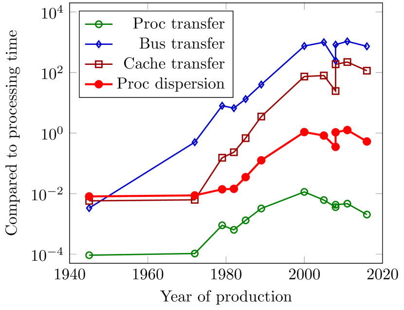
Figure 1: The history of some relative temporal characteristics of processors, in function of their production year. Notice how cramming more transistors in a processor changed their temporal characteristics disadvantageously.

3.2 The case of integrated circuits

We derive dispersion for integrated circuits in the same way as discussed for vacuum tubes. Fig. 1 shows the dependence of different dispersion values on the year of fabrication of the processor. The technical data are taken from publicly available data and from [14]. The figures of the merits are rough and somewhat arbitrary approximations. However, their consequent use enables us to draw limited validity conclusions without needing proprietary technological data.

We estimate the distance between the processing elements in two different ways. We calculate the ”average distance” of the transistors (the ”best case”) as the square root of the processor area divided by the number of transistors, and we consider it as a minimum distance the signals must travel between transistors. This value, divided by the clock frequency, is depicted as ”Proc transfer” in Fig. 1. The maximum distance between the two farthest processing elements on the chip, which is the processor area’s square root.

As the ”Proc dispersion” diagram line shows, in today’s technology the dispersion is near to unity. That is, we cannot apply the ”dispersionless” classic paradigm any more. Furthermore, this means that the operating regime of our today’s processors are more close to the operating regime of our brain (where explicit ”spatiotemporal” behavior is considered and is ”unsound” to use the classic paradigm to describe it) than the operating principle abstracted in the classic paradigm.

As we experience it, since the dispersion approached unity about two decades ago, only a small fragment of the input power can be used for computation; the rest of it is dissipated (produces only heat). The dispersion of synchronizing the computing operations vastly increases the cycle time, decreases the utilization of all computing units, and enormously increases the power consumption of computing [16, 17]. It is one of the major reasons for the inefficiency [18] of the ASIC circuits, and led to the symptom that moving data requires more energy [19] than manipulating it. The increased dispersion enormously decreases performance as the complexity and the relative transfer-to-processing time increases.

3.3 The case of technology blocks

Given that the processing elements and the storage elements usually are fabricated as separated technological blocks, and they are connected by wires (aka bus), we also estimated a ”bus transfer” time. The memory access time in this way is extended by the bus transfer time. We assumed that a cache memory is positioned at a(n average) distance of half processor size because of this effect. This time is shown as ”Cache transfer” time. The cache memories appeared about the end of the 1980s, when it became evident that the bus transfer drastically increases the memory transfer time (cache data can be calculated for all processors, however).

An interesting parallel is that both EDVAC and Intel 8008 have the same number of processing elements, and also the relative derived processor and cache transfer times are in the same order of magnitude. However, notice that the bus transfer time’s importance has grown and started to dominate the single-processor performance in personal computers. A decade later, the physical size of the bus necessitated to introduce cache memories. The physical size led to saturation in all relative transfer times. The slight decrease in the relative times in the past years can probably be attributed to the sensitivity of our calculation method to the spread of multi-cores; this suggests to repeat our analysis method with proprietary technological data.

3.4 The need for communication

Also, at the time when von Neumann proposed his paradigm, there was literally only one processor. Because of this, questions how it will communicate and cooperate with the rest of (computing) world, should not be asked: there was no external world and no other processor. Today, billions of processors are fabricated in every year. They use ad-hoc methods and ideas about cooperation and communication; furthermore, they use their payload time for that activity. Furthermore, that activity increases the non-parallelizable portion of the tasks. It is very desirable to extend computing paradigm with considering the presence of other processors.

3.5 Using new physical effect/ technology/ material in the computing chain

Given that the total execution time also comprises the transfer time, the meaningful analysis must consider the full time budget of the computing operations.

3.5.1 Using memristors for processing

A recently proposed idea is to replace slow digital processing with quick analog processing [20, 21], and may be proposed using any future new physical effect and/or material. Similar analysis can be followed in connection with the new physical effects considered in [22]: they decrease the physical processing time, only. To make them useful for computing, their in-component transmission time and especially the inter-component transmission time must be considerably decreased.

It sounds good that ”The analog memristor array is effectively the neural network laid out in the form of a crossbar, which can perform the entire operation in one clock cycle” [13]. In brackets, however fairly added, that (not counting the clock cycles that may be required to fetch and store the input and output data). Yes, the full story is that all operands of the memristor array must be transferred to its input (and previously, must be produced), and the results must be transferred to their destination; usually through a (high speed) serial bus. The total time of the memristor-related operations shall be compared to the total time of conventional operations to make a fair comparison.

3.5.2 Half-length operands vs. double-length ones

The mutual locking of the transfer (and other, non-immediately payload operations) and the payload operations similarly leads to disappointing efficiency improvement when one attempts to use half-length operands instead of double-length ones. The expectation behind the idea is that the shorter operand length may increase by a factor of four the desperately low efficiency of the artificial intelligence class applications running on supercomputers. One expects a four-fold performance increase when using half-precision rather than double-precision operands [23], and the power consumption data underpin that expectation. However, the measured increase in computing performance was only three times higher: their temporal behavior limits the utility of using shorter operands, too. The housekeeping (such as fetching, addressing, incrementing, branching) remained the same, and because of the mutually blocking nature of the payload-non-payload operations, the increase of the payload performance is significantly lower. In the case of AI-type workload, the transfer time is significantly higher (the housekeeping can be neglected apart from transfer time), so the performance with half-precision and double precision operands differ only marginally. For details, see [24, 25].

3.5.3 The role of transfer time

The relative weight of the data transfer time has grown tremendously for many reasons. Firstly, miniaturizing processors to sub-micron size while keeping the rest of the components (such as buses) above the centimeter scale. Secondly, single-processor performance has stalled [26], mainly because of reaching the limits, the laws of nature enable [27] (but, as we present, also because of tremendously extending its inherent idle waiting times). Thirdly, making truly parallel computers failed [3], and we can reach the needed high computing performance only through putting together an excessive number of segregated processors. This latter way replaced parallel computing with parallelized sequential computing (aka distributed computing), disregarding that the operating rules of the latter [28][29][24] sharply differ from those experienced with segregated processors. Fourthly, the utilization mode (mainly multitasking) forced us to use an OS, which imitates a ”new processor” for a new task, at serious time expenses [30][31]. Finally, the idea of ”real-time connected everything” introduced geographically large distances with their corresponding several millisecond data transfer times. Despite all of this, the idea of non-temporal behavior was confirmed by accepting the idea of ”weak scaling” [32], suggesting that all housekeeping times, such as organizing the joint work of parallelized serial processors, sharing resources, using exceptions and OS services, delivering data between processing units and data storage units, are negligible.

3.5.4 How the presence of transfer time was covered

The experience showed that even within the core, wiring (and its related transfer time) has an increasing weight [27] in the timing budget. When reaching the technology limit about $200~{}nm$ around the year 2000, wiring started to dominate (compare this date to the year when saturation is reached in Fig. 1). Further miniaturization can enhance the computing performance only marginally but increases the issues due to approaching the limiting interaction speed, as discussed below.

It is accepted that logical gates have an operating time, and to compensate for the different number of gates on different paths, functionally not needed (such as invert-reinvert) gates are inserted on the path with fewer gates. The design comprises several clock domains, and some bigger parts of the design run with different synchronization. These solutions can more or less compensate for the evident time difference. However, on one side, computing systems ”have a clock signal which is distributed in a tree-like fashion into every tiny part of the chip…Approximately 30 % of the total consumption of a modern microprocessor is solely used for the clock signal distribution.” [16] It was the case 10 years ago, so for today, we can assume 50% (and about the same amount of power is needed for cooling). On the other side, the difference in the length of physical signal paths causes a ”skew” of the signals, which became a major challenge in designing high-performance systems. It leads to additional performance loss (mainly due to the dispersion of the clock signal needed to synchronize the computing operations [33]). Even inside the die: the segregated processors have very low efficiency [18]. Despite this, today, wafer (and even multi-wafer [34]) sized systems are also under design and in use.

In complete systems, such as supercomputers running HPCG workload, only 0.3 % of the consumed energy goes for computing, and this proportion is getting much worse if conventional systems attempt to mimic biology, such as to run an ANN workload. The poor understanding of basic terms of computing resulted in that in supercomputing ”the top 10 systems [of TOP500] are unchanged from the previous list” [35], and that ”Core progress in AI has stalled in some quite different fields” [36]; from brain simulation [37] to ANNs [38]; in general, the AI progress [36] as a whole.

3.6 The case of non-negligible transfer time

At his time and in the age of vacuum tube technology, von Neumann did not feel the need to discuss what a procedure can justify describing the computing operation in a non-dispersionless case. However, he suggested reconsidering the validity of the neglections he used in his paradigm for any new future technology. To have a firm computing paradigm for the present technologies, we need to consider the ratio of the transfer time to processing time; we cannot neglect it anymore. The real question [33] is, the discussion of which is missing from the ”First draft”, what a procedure shall be followed if the transfer time is not negligible?

4 The time-space system

4.1 Considering the transfer time

Although von Neumann explicitly mentioned that the propagation speed of electromagnetic waves limits the operating speed of the electronic components, until recently, that effect was not admitted in computing. In contrast, in biology, the ”spatio-temporal” behavior [39] was recognized very early. In both technical and biology-related computing, the recent trend is to describe computing systems theoretically and model their operation electronically using the computing paradigm proposed by von Neumann, which is undoubtedly not valid for today’s technologies. Furthermore, as mentioned above, our computing devices’ operating regime is closer to that of our brain than to the abstract model. That is, a similar description for both the computer and the brain would be adequate.

Fortunately, the spatio-temporal behavior suggests a ”procedure” that can be followed in the case when the transfer time can even be longer than the processing time, the case which is missing from the ”First Draft” [33]. Although biology –despite the name ”spatio-temporal”– describes the behavior of its systems using separated space and time functions (and as a consequence, needs ad-hoc suggestions and solutions for different problems), it has one common attribute with technical computing: in both of them, the information transfer speed is limited. Because of its physical (and maybe philosophical) relevance, a more detailed explanation is given in [40].

For the first look, it seems to be strange to describe such systems with (the inverse of) the Minkowski transform, given that it became famous in connection with Einstein’s theory of special relativity. However, in its original form, only the existence of a limiting speed is assumed. This latter feature enables us to describe the correct behavior of information processing in science-based technological implementations and biology for any combination (ratio) of the transfer time and the processing time. The key idea is to transform the spatial distances between computing components (that can be $Si$ gates, cores, network nodes, biological or artificial neurons) to time (measured with the limiting speed along the signal path).

We only assume that a limiting speed exists and that transferring information in the system needs time. In our approach, Minkowski provided a mathematical method to describe information transfer phenomena in a world, where the interaction speed is limited. The only new assumptions we make are that the events also have a processing time, such as an atomic transition, executing a machine instruction, or issuing/receiving a neural spike; furthermore, the interaction speed is other than the speed of light.

Special relativity describes the space around us with four-dimensional space-time coordinates, and calculates the fourth spatial coordinate from the time as the distance the light traverses in a given time; simply because around us the distance was the easily accessible, measurable quantity – hundred years ago.

In computing, distances get defined during the fabrication of components and assembling the system. They may be different in different systems; however, they must meet their timing constraints. In biological systems, nature defines neuronal locations and distances, and in ’wet’ neuro-biology, signal timing rather than axon length is the right (measurable) parameter. To introduce temporal logic (meaning: the logical value of an expression depends on WHERE and WHEN is it evaluated) into computing, the reverse of the Minkowski transformation is required: the time, rather than the position, is the primary measurable quantity. We need to use a special four-vector, where all coordinates are time values: the first three are the corresponding local coordinates (divided by the speed of interaction), having a time dimension. The fourth coordinate is the time itself. Distances from an event’s location are measured along their access path; they are not calculated from their corresponding spatial coordinates.

In the case of electronics, the limiting speed is connected to the speed of light (in biological systems, the case is more complicated, but the speed of interaction is finite, anyhow). Given that we use the time as the primary variable, the formalism can also be used to describe neuronal operation (where the conduction speed is modulated) with time, rather than space. However, in the latter case, the formalism is less straightforward. At the same time, the famous hypothetical experiment can be excellently described in our time-space system, too. With that experiment we demonstrate, that the solid mathematical background provided by the Minkowski-transform (and all associated behavior of modern science, also describing modern technological materials) is preserved. In the following chapters we use the transformed coordinates only to describe the temporal behavior of computing systems.

That is, the only change introduced to logic functions of computing is that they are not any more evaluated implicitly at point (0,0,0,0). Instead, they are evaluated at a point (x,y,z,t) of the time-space. Below, we introduce the idea and its notations. Through describing the famous hypothetic experiment, we demonstrate that our time-space system is equivalent to the commonly used space-time systems. The validity and the mathematical features of the latter have been scrutinized exclusively in the past 140 years. So, on one side, we use the solid background the computer science is based upon: mathematics; on the other side, we extend it with the similarly solid background of time-space formalism.

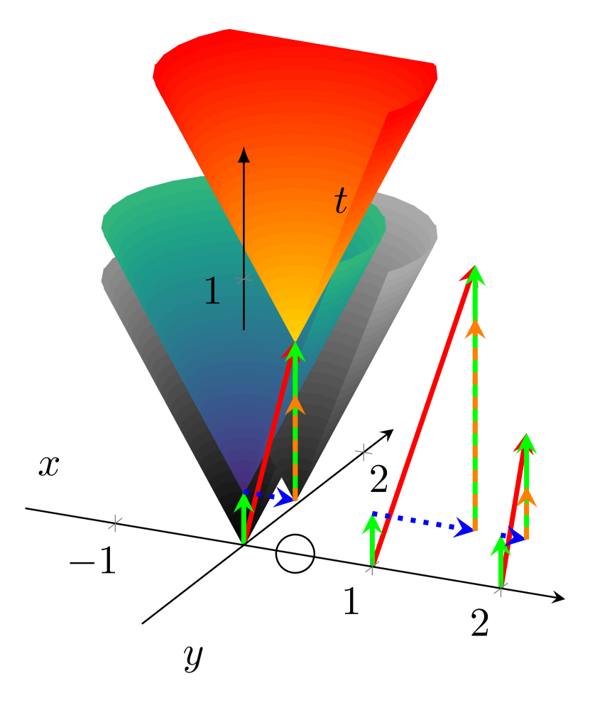
Figure 2: The computing operation in time-space approach. The processing operators can be gates, processors, neurons, or networked computers. The ”idle waiting time”, rooting in the finite interaction speed and the physical distance of computing elements (see mixed-color vectors in figure), is one of the major sources of computing systems’ inefficiency.

4.2 Introducing the time-space system

With the reasoning above, we introduce [40] a four dimensional time-space system. The resemblance with the Minkowski space is evident, and the name difference signals the different utilization methods.

In our particular coordinate system (used in some figures below), formally (x,y,t) coordinates are used (for better visibility, the third spatial coordinate is omitted). What happens at time $t$ in a computing component at position (x,y) happens along a line parallel with axis $t$, along a line perpendicular to plane at (x,y). The objects are annotated with their spatial position coordinates ’x’ and ’y’, but they are time values: how much time the signal having the limiting speed needs to reach that point. Several ’snapshots’ taken at time $t$ about the same computing object are shown in the 3-D figures, on top of each other. The computing objects may alternatively be positioned at some arbitrary position that corresponds to the same time distance from point (0,0,0) (a cylindrical coordinate system would be adequate but would make both visualization and calculations much harder to follow).

The arrows in the same horizontal plane represent the same time (no transmission). The interaction vectors are neither parallel with the time axis nor are in a spatial plane: both their temporal and spatial coordinates change as the interaction propagates. In electronic systems, the speed of interaction is constant, so the vectors are simple lines. Those spatial vectors are displayed with their different projections in the corresponding figures, enabling their easy trigonometric calculation. Their physical (spatial) length corresponds to the physical time between their endpoints. The horizontal blue arrows are just helper lines: the position (annotated by x,y, but denoting the time the signal from (0,0,0) needs to reach this position) is projected to time axes $x$ and $y$ (the XY plane). The red arrow is the vectorial sum of the two projections, also in that plane.

At the positions in the (x,y) plane, the events happen at the same time (although the other processing units will be able to notice that at a correspondingly later time, i.e., in another XY plane), and the events happening in connection with a processing unit, are aligned on an arrow parallel with axis $t$. In this sense, we can interpret ’classic computing’: our objects are compressed to one single XY plane: all events, at all objects, happen simultaneously. Even as the time distance between our computing objects is zero, because of the instantaneous transmission (independently from its technical implementation), the figure shall be represented with a mathematical point at (0,0,0). The processing time is only an engineering imperfectness, according to the ’classic computing science’.

4.3 Validating the time-space system

Figure 2 (essentially a light cone in 2D space plus a time dimension) on one side demonstrates that our reversed Minkowski transform is equivalent for discussing the famous hypothetic experiment of relativity with the original transform, on the other side shows why time must be considered explicitly in all kinds of computing. The figure shows that an event appears in our time-space system at point (0,0,0). The only (very plausible) difference to the classic hypothetic experiment is that we assume that signaling needs some time, too (not only the interaction, but also its technical implementation needs time). Our observers (fellow computing objects) are located on the ’x’ axis; the vertical scale corresponds to time. In the classic physical hypothetical experiment, a light is switched on in the origo: the need to perform a calculation appears. The observers switch their light on (start their calculation) when they notice that the first light is switched on (the instruction/operand reaches their position). The distance traveled by the light (the signal carrying the instruction) is given as the value of time multiplied by the speed of light (signal speed). At any point in time on the vertical axis, a circle describes the propagation of light (signal). In our (pseudo) 3-dimensional system, the temporal behavior is described as a conical surface, known as the future light cone in science.

Both light sources (computing objects) have some ’processing time’, that passes between noticing the light (receiving an instruction/operand) and switching their light (performing an instruction). An instruction is received at the bottom of the green arrow. The light goes on at the head of the arrow (i.e., at the same location, but at a later time) when the ’processing time’ $T_{p}$ passed. Following that, the light propagates in the two spatial dimensions as a circle around the axis ’t’. Observers at a larger distance notice the light at a later time: a ’transmission time’ $T_{t}$ is needed. If the ’processing time’ of the light source of our first event were zero, the light would propagate along the gray surface at the point (0,0,0). However, because of the finite processing time of the source, the signal propagates along the blueish cone surface, at the head of the green arrow.

A circle marks the position of our other computing unit on the axis ’x’. With zero ’transmission time’, a second gray conical surface (at the head of the horizontal blue dotted arrow) would describe the propagation of its signal. However, this second ’processing time’ can only begin when our second processing unit receives the instruction at its position: when the mixed-color vertical dashed arrow hits the blueish surface. At that point begins the ’processing time’ of our second processing unit; the yellowish conical surface, beginning at the second vertical green arrow, describes the second signal propagation. The horizontal (blue dotted) arrow describes the physical distance of the second computing unit (as a time coordinate) from the first one, the vertical (mixed color dashed) arrow describes the time delay of the instruction. It comprises two components: $T_{t}$ transmission time (mixed color) to the observer unit and its $T_{p}$ processing time (green). The light cone of the observer (emitting the result of calculation) starts at $t=2*T_{p}+T_{t}$.

The red arrow represents the resulting apparent processing time $T_{A}$: the longer is the red vector; the slower is the system. As the vectors are in the same plane, $T_{A}=\sqrt{T_{t}^{2}+(2\cdot T_{p}+T_{t})^{2}}$, that is $T_{A}=T_{p}\cdot\sqrt{R^{2}+(2+R)^{2}}$. The apparent time is a non-linear function of both of its component times and their ratio $R$. If more computing elements are involved, $T_{t}$ denotes the longest transmission time. (Similar statement is valid if $T_{p}$ times are different.) The effect is significant: if $R=1$, the apparent execution time of performing the two computations is more than three times longer than $T_{p}$.

Two more observers are located on the axis ’x’, at the same position, to illustrate the influence of transmission speed (and/or ratio $R$). For visibility, their timings are displayed at points ’1’ and ’2’, respectively. In their case the transmission speed differs by a factor of two compared to that displayed at point ’0’; in this way three different $R=T_{t}/T_{p}$ ratios are used. Notice that at half transmission speed (the horizontal blue arrow is twice as long as the one at the origo) the vector is considerably longer, while at double transmission speed, the decrease of the time is much less expressed.

4.4 Scrutinizing the temporal behavior

The temporal behavior means that the value of logical functions depends on both time and place of evaluating the corresponding logical function.

Notice that some consequences are stemming immediately from the nature of our model. Now two computing elements are sitting at point(0,0,0) and (0,1,0). The second element calculates something that expects the calculation of the first element as its input operand of the second calculation. Consider that the result is inside the green arrow during its processing time and comes to light after that time. As visible from the discussion and the figure, the first event happens at a well-determined position and time values in our space-time system. Its spatial coordinates agree with those of the spatial position of the first element. Furthermore, they are different from those of the second element: the result must be transported: it shall be delivered to the position of the second processing unit.

The event starts to propagate, and its final destination’s coordinates differ both in time and space from those of the origin. It would be described as positioned at the head of the red vector (such vectors are neither vertical vectors, parallel with the $t$ axis, nor lie within the plane (x,y) ). During this transfer, the space coordinate (the projection of the time-space distance to the (x,y) plane) changes to the coordinates of the head of the blue arrow: here was the observer when the event happened. In the meantime, however, the time passed for the observer, and now the vertical arrow at its position describes its coordinate. That vertical arrow comprises two contributions: the upper green arrow represents the processing time of the observer, and we also have the length of the mixed-color arrow (the idle waiting): it has the same length as the blue dotted arrow: our observer must wait for such a long time to receive the signal. Given that all signals are in the plane (x,t), the actual time distances can be calculated straightforwardly. The projection of the event to axis $t$ is $T_{p}+T_{i}+T_{p}$, that is the apparent processing time includes idle time $T_{i}$, that equals to the transfer time between the two processing units.

From our observation point, we see that the delivery times are considerably higher than those based on summing projections to the $t$ axis. Using different words, the apparent execution time in our a time-space system is indeed more prolonged than the time difference calculated based on only the values projected to the $t$ axis. The difference (the length of the blue arrow) depends on the distance of the objects along the axis $x$ and the system’s interaction speed. The figure suggests that the difference is the larger, the more complex operations are involved, and the larger is the physical size of the system (provided that the system defines the interaction speed). The primary result of that transformation is that the apparent processing time can be calculated by using simple geometrical relations.

When looking at the events from the direction of the $x$ axis in the (x,t) plane, we see that the total time corresponds to the sum of the two processing times in’ classic computing’. The waiting time of the second unit is only an arrowhead (instant interaction). It denotes the corresponding logical dependence but does not increase processing time. The second unit must wait for the result of the first calculation because of their logical dependence. However, because of instant delivery, no additional waiting is required. Consequently, according to the ”timeless (classical) paradigm, ” observers’ distance seems to be zero. The introduced extra dimension, time of interaction, changes the picture drastically. The closer is the difference between the summed length of the two green vectors to the red vector’s length; the larger is the speed of their interaction. They are equal, however, only if the interaction speed is infinitely large.

4.5 Computing efficiency as a consequence of temporal behavior

It has been discussed virtually infinite times in computing that the computing performance depends on many factors. However, the temporal dependence has never been included. As the discussion above suggested, time has a decisive role in computing; the idle waiting times indeed degrade performance, so the rest of the discussion shall focus on the role of time in shaping performance.

Given that the spatial distance is equivalent to time, they have a similar role. The processor operation itself has some idle time, and, as discussed in the next sections, the outdated technical principles and solutions add more (and slightly different) idle times. Moore’s observation is valid only for the gate’s density inside chips, but not for the components (such as buses) connecting them, so the idle (transmission) time increases. This relation has a self-exciting effect: the low efficiency (that decreases as the required performance increases) means that a larger portion of energy consumption is used for heating (and because of that: needs more cooling), needing more physical space, which increases the physical distance of components, causing worse performance, and so on.

On one side, the communication between processors is implemented in a way that increases the non-payload, sequential-only portion of the task. On the other side, the physical time of transmission (that depends on both the speed of interconnection and the physical distance between the corresponding computing objects) also significantly contributes to degrading the efficiency. Also, the algorithms, how the components are used, and the parameters of the architecture all impact the system’s computing efficiency. The benchmark data of the components define the hard limits, and their way of cooperation the soft limits that can be experienced. That is, the temporal behavior of their components is a vital feature of computing systems, especially of the excessive ones, mainly if they target high computing performance, especially if they are running very demanding workloads.

5 Technical solutions for the vacuum-tube age

Some of the ”classic” technical implementations, that – due to the incremental development – survived their technical state-of-the-art, and (especially in the light of temporal analysis) need drastic revision. Also, research is going on (both in science and technology, with vast investments in the background) to find new materials/effects/technologies. However, science severely limits their usability: the temporal analysis provides a helping hand also here, enabling optimizing performance/cost. ”Reinventing electronics”[12] is necessary not only for computing devices but also their interconnection and modes of utilization.

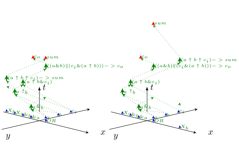
Figure 3: The temporal dependence diagram of a 1-bit adder. The diagram shows the logical equivalent of the SystemC source code of Listing 1, the lack of vertical arrows signals ”idle waiting” time (undefined gate output) Left side: the second XOR gate is at (-1,0). Right side: the second XOR gate is at (+1,0). Notice how changing the position of a gate affects signal timing.

5.1 Method of identifying bottlenecks of computing

The transmission time $T_{t}$ is an ’idle time’ from the point of view of computing: the component is ready to run, takes power, but does no useful work. Due to their finite physical size and the finite interaction speed (both neglected in the classic paradigm), the temporal operation of computing systems results inherently in an idle time of the Processing Units, that can be a significant contributor to non-payload portion of their processing time. Given that the different apparent processing times inevitably increase the dispersion, they can be a key factor of the experienced inefficiency of general-purpose chips [18]. With other major contributors, originating from the technical implementation of their cooperation, these ”idle waiting” times sharply decrease the payload performance of computing systems. It is worth to discuss the inside-component and inter-component contributions separately.

In the spirit of the temporal behavior, we can set up two general classes of processing: the payload processing $T_{p}$ makes our operations directly related to our goal of computation; all other processing is counted as non-payload processing. The merit we use is the time spent with that processing. As will be shown, some portion of the non-payload processing time roots in laws of nature: computing inherently includes idle times, some other portion (such as housekeeping) is not directly useful. However, any kind of processing takes time and consumes energy. The task of designing our computing systems is to reduce the total processing time, i.e., to develop solutions that minimize the proportion of the ’idle’ activity; not only at a component level but also at the system level. Scrutinizing the temporal diagrams of components, solutions, and principles is an excellent tool to find bottlenecks.

In the figures below, near to (vertical) axis t are shown vertical arrows (where payload processing happens) or lack of arrows (when non-payload processing occurs). The large amount of non-payload processing (that increases with system complexity) explains the experienced low computing efficiency of computing systems using those technical implementations. The proportions of times are chosen for better visibility and call attention to its effect rather than reflect some realistic arrangements.

5.2 Gate-level processing

Although for its end-users, the processor is the ”atomic unit” of processing, principles of computing are valid also at ”sub-atomic” level, at the level of gate operations. Describing the temporal operation at gate level is an excellent example, that the line-by-line compiling (sequential programming, called also Neumann-style programming [41]), formally introduces only logical dependence, but through its technical implementation it implicitly and inherently introduces a temporal behavior, too.

The one-bit adder is one of the simplest circuits used in computing. Its typical implementation comprises 5 logic gates, 3 input signals, and 2 output signals. Gates are logically connected internally: they provide input and output for each other. The relevant fraction of the equivalent source code is shown in Listing 1.

Listing 1: The essential lines of source code of the one-bit adder implemented in SystemC

⬇

//We are making a 1-bit addition

aANDb = a.read() & b.read();

aXORb = a.read() ^ b.read();

cinANDaXORb = cin.read() & aXORb;

//Calculate sum and carry out

sum = aXORb ^ cin.read();

cout = aANDb | cinANDaXORb;

Fig. 3 shows the timing diagram of a one-bit adder, implemented using common logic gates. The three input signals are aligned on axis $y$; the five logic gates are aligned on axis $x$. Gates are ready to operate, and signals are ready to be processed (at the head of the blue arrows). The logic gates have the same operating time (the length of green vectors); their access time distance includes the needed multiplexing. The signals must reach their destination gate (dotted green arrows), that (after its operating time passes) produces the output signal, that starts immediately towards the next gate. The vertical green arrows denote gate processing (one can project the arrow to axis $x$ to find out the gate’s ID), labeled with the produced signal’s name. Because of the non-synchronized operating mode, there are ”pointless” arrows in the figure. For example, signal $a\&b$ reaches the $OR$ gate much earlier than the signal to its other input. Depending on the operands of $OR$, it may or may not result in the final sum. The gates always have an output signal, even if they did not receive their expected input.

Notice that considering the physical distance and the finite interaction speed drastically changes the picture we have (based on ”classic computing”), that the operating time of the adder is simply the sum of the ”gate times”. For example, the very first AND and XOR operations could work in parallel (at the same time), but the difference in their physical distance the signals must travel, changes the times when they can operate with their signals. Also, compare the temporal behavior of the signal $sum$ on the two figures. The only difference between subfigures is that the second XOR gate moved to another place.

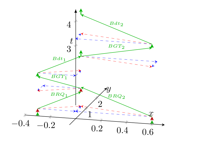
Figure 4: The computing operation in time-space approach. The processing operators can be gates, processors, neurons, or networked computers. The ”idle waiting time”, rooting in the finite interaction speed and the physical distance of computing elements (see mixed-color vectors in figure), is one of the major sources of computing systems’ inefficiency.

5.3 The serial bus

Fig. 4 discusses, in terms of ”temporal logic”: why using high-speed buses for connecting modern computer components leads to very severe performance loss, especially when one attempts to imitate neuromorphic operation. The processors are positioned at (-0.3,0) and (0.6,0). The bus is at a position (0,0.5). The two processors make their computation (green arrows at the position of processors), then they want to deliver their result to its destination. We assume that they want to communicate simultaneously. First, they must have access to the shared bus (red arrows). The core at (-.3,0) is closer to the bus, so its request is granted. As soon as the grant signal reaches the requesting core, the bus operation is initiated, and the data starts to travel to the bus. As soon as it reaches the bus, the bus’s high speed forwards it, and at that point, the bus request of the other core is granted, and finally, the calculated result of the second core is bused.

At this point comes into picture the role of the workload on the system: we presumed that the two cores want to use the single shared bus, at the same time, for communication. Given that they must share it, the apparent processing time is several times higher than the physical processing time. Moreover, it increases linearly with the number of cores connected to the bus, if a single high-speed bus is used. In vast systems, especially when attempting to mimic neuromorphic workload, the bus’s speed is getting marginal. Notice that the times shown in the figure are not proportional: the (temporal) distance between cores is in the several picoseconds range, while the bus (and the arbiter) are at a distance well above nanoseconds, so the actual temporal behavior (and the idle time stemming from it) is much worse than the figure suggests. This behavior is why ”The idea of using the popular shared bus to implement the communication medium is no longer acceptable, mainly due to its high contention.” [42]. For a more detailed analysis see [40], and specifically for the case of artificial neural networks [25]. The figure suggests using another design principle instead of using the bus exclusively, directly from the computing component’s position.

When using a shared bus, increasing either the processing speed or the communication speed, alone, does not affect linearly the total execution time any more. Furthermore, it is not the bus speed that limits performance. A relatively small increase in the transfer time $T_{t}$ can lead to a relatively large change in the value of the apparent processing time $T_{A}$. This change leads to an incomprehensible slowdown of the system: its slowest component defines its efficiency. The conventional method of communication may work fine as long as there is no competition for the bus, but leads to queuing of messages in the case of (more than one!) independent sources of communication. The effect is topped by the bursty nature of communication caused by the need for central synchronization, leads to a ”communicational collapse” [43], that denies huge many-processor systems, especially neuromorphic ones [44].

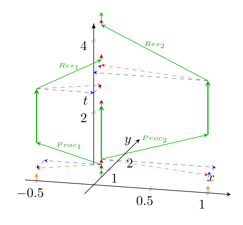
Figure 5: The operation of the ”parallelized sequential” processing, in the time-space coordinate system. Parallel with axis t, the lack of vertical arrows signals ”idle waiting” time, both for the coordinator and the fellow processors

5.4 Distributed processing

Given that single-processor performance stalled [2], and building parallel computers failed [3], to reach the needed high computing performance, the computing tasks must be cut into pieces and be distributed between independently working single processors. Cutting and re-joining pieces, however, needs efforts both from programming and technology. The technology, optimized for solving single-thread tasks, hits back when several processors must cooperate, as cooperation and communication are not native features of segregated processors. The task was so hard that the famous Gordon Bell Prize [45] was awarded initially to achieve an at least 200-fold performance gain via distributing a task between several (even thousands of) processors.

Fig 5 depicts the time diagram of distributed parallel processing. One of the Processing Units (in our case, the one at (0,0.5)) orchestrates the operation, including receiving the start command and sending the result. This core makes some sequential operations (such as initializing data structures, short green arrow), then it sends the start command and operands to fellow cores at (-0.5,0) and (1,0), one after the other. Signal propagation takes time (depending on distance from the coordinator). After that time, fellow cores can start their calculation (their part of the parallelized portion). Of course, the orchestrator Processing Unit must start all fellow Processing Units (red arrows), then it can start its portion of distributed processing.

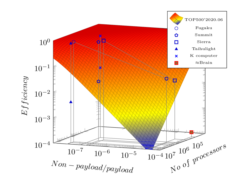
Figure 6: The 2-parameter efficiency surface (in function of the parallelization efficiency measured by benchmark HPL and the number of the PUs) as concluded from Amdahl’s Law (see [24]), in the first order approximation. Some sample efficiency values for some selected supercomputers are shown, measured with benchmarks HPL and HPCG, respectively. Also, the estimated efficacy of brain simulation using conventional computing is shown.

As the fellow Processing Units finish their portion, they must transmit their data $Res_{i}$ to the orchestrator, that receives those data in sequential mode, and finally makes some closing sequential processing. Again, the inherently sequential-only portion [46] of the task increases with number of cores and its idle waiting time (time delay of signals) increases with physical size (cable length). Notice also that the orchestrating Processing Unit must wait for the results from all fellow cores, i.e., the slowest branch defines performance. This aspect is significant, if the physical transmission times of those units differ (speed or distance is different), the task is not adequately split into equal portions. Modern hardware has undeterministic behavior [47][48], or the units are connected through an interconnection with stochastic behavior [49]. The times shown in the figure are not proportional and largely depend on the type of the system. For a detailed discussion, see [24].

The dispersion in distributed systems is dramatically increased because of the physical distance of the computing components. The increase depends on the weight of the critically large distances. As analyzed in detail in [24], the different communication intensity increases the weight of the operation having a considerable temporal distance. For vast distributed systems, see Fig.6, the efficiency sharply depends on the number of parallelized units and the goodness of their parallelization. ”This decay in performance is not a fault of the architecture, but is dictated by the limited parallelism” [28]

6 Conclusion

The technological development made the neglections used in the commonly used computing model outdated and forces us to consider the original model, with correct timing relations. The stealthy nature of the development led to many technological implementations, including the synchronous operation and the high-speed bus that are not usable anymore. One obvious sign is the enormous dissipation of our computing systems, which is a direct consequence of the fact that the computing systems’ dispersion is well above the theoretically acceptable level. ”Reinventing electronics” [12] is a must, and not only for building neuromorphic computing devices. The computing model is perfect, but the classic paradigm is used far outside its validity range. For today’s technological conditions, the needed ”contract” [3] between mathematics and electronics, should be based on a paradigm that considers the transfer time.

References

- [1] J. von Neumann, “First Draft of a Report on the EDVAC,” https://web.archive.org/web/20130314123032/ http://qss.stanford.edu/ godfrey/vonNeumann/vnedvac.pdf, 1945.
- [2] S. H. Fuller and L. I. Millett, Eds., The Future of Computing Performance: Game Over or Next Level? National Academies Press, Washington, 2011.
- [3] K. Asanovic, R. Bodik, J. Demmel, T. Keaveny, K. Keutzer, J. Kubiatowicz, N. Morgan, D. Patterson, K. Sen, J. Wawrzynek, D. Wessel, and K. Yelick, “A View of the Parallel Computing Landscape,” Comm. ACM, vol. 52, no. 10, pp. 56–67, 2009.
- [4] S(o)OS project, “Resource-independent execution support on exa-scale systems,” http://www.soos-project.eu/index.php/related-initiatives, 2010.
- [5] Machine Intelligence Research Institute, “Erik DeBenedictis on supercomputing,” 2014. [Online]. Available: https://intelligence.org/2014/04/03/erik-debenedictis/
- [6] J. Sawada et al, “TrueNorth Ecosystem for Brain-Inspired Computing: Scalable Systems, Software, and Applications,” in SC ’16: Proceedings of the International Conference for High Performance Computing, Networking, Storage and Analysis, 2016, pp. 130–141.
- [7] M. D. Godfrey and D. F. Hendry, “The Computer as von Neumann Planned It,” IEEE Annals of the History of Computing, vol. 15, no. 1, pp. 11–21, 1993.
- [8] C. D. S. et al, “A Survey of Neuromorphic Computing and Neural Networks in Hardware,” 2017.
- [9] W. Aspray, John von Neumann and the Origins of Modern Computing. MIT Press, Cambridge, 1990, pp. 34–48.
- [10] S. K. et al, “Acceleration of an asynchronous message driven programming paradigm on ibm blue gene/q,” in 2013 IEEE 27th International Symposium on Parallel and Distributed Processing. Boston: IEEE, 2013. [Online]. Available: https://https://ieeexplore.ieee.org/abstract/document/ 6569854
- [11] Steve Furber and Steve Temple, “Neural systems engineering,” J. R. Soc. Interface, vol. 4, pp. 193–206, 2007.
- [12] D. Markovic, A. Mizrahi, D. Querlioz, and J. Grollier, “Physics for neuromorphic computing,” Nature Reviews Physics, vol. 2, pp. 499–510, 2020.
- [13] J. D. Kendall and S. Kumar, “The building blocks of a brain-inspired computer,” Appl. Phys. Rev., vol. 7, p. 011305, 2020.
- [14] J. J. P. Eckert and J. W. Mauchly, “Automatic High-Speed Computing: A Progress Report on the EDVAC,” Moore School Library, University of Pennsylvania, Philadephia, Tech. Rep. Report of Work under Contract No. W-670-ORD-4926, Supplement No 4, September 1945.
- [15] M. Schlansker and B. Rau, “EPIC: Explicitly Parallel Instruction Computing,” Computer, vol. 33, no. 2, pp. 37–45, Feb 2000.
- [16] R. Waser, Ed., Advanced Electronics Materials and Novel Devices, ser. Nanoelectronics and Information Technology. Wiley, 2012.
- [17] H. Esmaeilzadeh, E. Blem, R. St. Amant, K. Sankaralingam, and et al., “Dark Silicon and the End of Multicore Scaling,” IEEE Micro, vol. 32, no. 3, pp. 122–134, 2012.
- [18] R. Hameed, W. Qadeer, M. Wachs, O. Azizi, A. Solomatnikov, B. C. Lee, S. Richardson, C. Kozyrakis, and M. Horowitz, “Understanding sources of inefficiency in general-purpose chips,” in Proceedings of the 37th Annual International Symposium on Computer Architecture, ser. ISCA ’10. New York, NY, USA: ACM, 2010, pp. 37–47. [Online]. Available: http://doi.acm.org/10.1145/1815961.1815968
-
[19]
H. Simon, “Why we need Exascale and why we won’t get there by 2020,” in
Exascale Radioastronomy Meeting, ser. AASCTS2, 2014. [Online].
Available: https://www.researchgate.net/publication/261879110
_Why_we_need_Exascale_and_why_we_won’t_get _there_by_2020 - [20] E. Chicca and G. Indiveri, “A recipe for creating ideal hybrid memristive-CMOS neuromorphic processing systems,” Applied Physics Letters, vol. 116, no. 12, p. 120501, 2020. [Online]. Available: https://doi.org/10.1063/1.5142089
- [21] “Building brain-inspired computing,” Nature Communications, vol. 10, no. 12, p. 4838, 2019. [Online]. Available: https://doi.org/10.1038/s41467-019-12521-x
- [22] P. C. et al., “Rebooting Our Computing Models,” in Proceedings of the 2019 Design, Automation & Test in Europe Conference & Exhibition (DATE). IEEE Press, 2019, pp. 1469–1476.
- [23] A. Haidar, P. Wu, S. Tomov, and J. Dongarra, “Investigating Half Precision Arithmetic to Accelerate Dense Linear System Solvers,” in Proceedings of the 8th Workshop on Latest Advances in Scalable Algorithms for Large-Scale Systems, ser. ScalA ’17. New York, NY, USA: ACM, 2017, pp. 10:1–10:8.
- [24] J. Végh, “Finally, how many efficiencies the supercomputers have?” The Journal of Supercomputing, vol. 76, no. 12, pp. 9430–9455, feb 2020. [Online]. Available: http://link.springer.com/article/10.1007/s11227-020-03210-4
- [25] J. Végh, “Which scaling rule applies to Artificial Neural Networks,” in Computational Intelligence (CSCE) The 22nd Int’l Conf on Artificial Intelligence (ICAI’20). IEEE, 2020, pp. Accepted ICA2246, in print; in review in Neurocomputing. [Online]. Available: http://arxiv.org/abs/2005.08942
- [26] US National Research Council, “The Future of Computing Performance: Game Over or Next Level?” 2011. [Online]. Available: http://science.energy.gov/ /media/ascr/ascac/pdf/meetings/mar11/Yelick.pdf
- [27] I. Markov, “Limits on fundamental limits to computation,” Nature, vol. 512(7513), pp. 147–154, 2014.
- [28] J. P. Singh, J. L. Hennessy, and A. Gupta, “Scaling parallel programs for multiprocessors: Methodology and examples,” Computer, vol. 26, no. 7, pp. 42–50, Jul. 1993.
- [29] J. Végh, “Re-evaluating scaling methods for distributed parallel systems,” IEEE Transactions on Distributed and Parallel Computing, vol. ??, p. Refused, 2020. [Online]. Available: https://arxiv.org/abs/2002.08316
- [30] D. Tsafrir, “The context-switch overhead inflicted by hardware interrupts (and the enigma of do-nothing loops),” in Proceedings of the 2007 Workshop on Experimental Computer Science, ser. ExpCS ’07. New York, NY, USA: ACM, 2007, pp. 3–3.
- [31] F. M. David, J. C. Carlyle, and R. H. Campbell, “Context Switch Overheads for Linux on ARM Platforms,” in Proceedings of the 2007 Workshop on Experimental Computer Science, ser. ExpCS ’07. New York, NY, USA: ACM, 2007. [Online]. Available: http://doi.acm.org/10.1145/1281700.1281703
- [32] J. L. Gustafson, “Reevaluating Amdahl’s Law,” Commun. ACM, vol. 31, no. 5, pp. 532–533, May 1988.
- [33] J. Végh, “von Neumann’s missing ”Second Draft”: what it should contain,” in The 2020 International Conference on Computational Science and Computational Intelligence; CSCI’20: December 16-18, 2020, Las Vegas, USA, paper CSCI2019. IEEE, 2020, p. paper CSCI2019. [Online]. Available: https://arxiv.org/
- [34] A. Grubl, S. Billaudelle, B. Cramer, V. Karasenko, and J. Schemmel, “Verification and Design Methods for the BrainScaleS Neuromorphic Hardware System,” Journal of Signal Processing Systems, vol. 92, pp. 1277–1292, 2020.
- [35] TOP500.org, “The top 500 supercomputers,” https://www.top500.org/, 2019.
- [36] M. Hutson, “Core progress in AI has stalled in some fields,” Science, vol. 368, p. 6494/927, 2020.
- [37] S. J. van Albada, A. G. Rowley, J. Senk, M. Hopkins, M. Schmidt, A. B. Stokes, D. R. Lester, M. Diesmann, and S. B. Furber, “Performance Comparison of the Digital Neuromorphic Hardware SpiNNaker and the Neural Network Simulation Software NEST for a Full-Scale Cortical Microcircuit Model,” Frontiers in Neuroscience, vol. 12, p. 291, 2018.
- [38] J. Keuper and F.-J. Preundt, “Distributed Training of Deep Neural Networks: Theoretical and Practical Limits of Parallel Scalability,” in 2nd Workshop on Machine Learning in HPC Environments (MLHPC). IEEE, 2016, pp. 1469–1476. [Online]. Available: https://www.researchgate.net/publication/308457837
- [39] J. Végh and Ádám J. Berki, “On the spatiotemporal behavior in biology-mimicking computing systems,” Brain Informatics, p. in review, 2020. [Online]. Available: https://arxiv.org/abs/2009.08841
- [40] J. Végh, “Introducing Temporal Behavior to Computing Science,” in 2020 CSCE, Fundamentals of Computing Science. IEEE, 2020, pp. Accepted FCS2930, in print. [Online]. Available: https://arxiv.org/abs/2006.01128
- [41] J. Backus, “Can Programming Languages Be liberated from the von Neumann Style? A Functional Style and its Algebra of Programs,” Communications of the ACM, vol. 21, pp. 613––641, 1978.
- [42] L. de Macedo Mourelle, N. Nedjah, and F. G. Pessanha, Reconfigurable and Adaptive Computing: Theory and Applications. CRC press, 2016, ch. 5: Interprocess Communication via Crossbar for Shared Memory Systems-on-chip.
- [43] S. Moradi and R. Manohar, “The impact of on-chip communication on memory technologies for neuromorphic systems,” Journal of Physics D: Applied Physics, vol. 52, no. 1, p. 014003, oct 2018.
- [44] S. B. Furber, D. R. Lester, L. A. Plana, J. D. Garside, E. Painkras, S. Temple, and A. D. Brown, “Overview of the SpiNNaker System Architecture,” IEEE Transactions on Computers, vol. 62, no. 12, pp. 2454–2467, 2013.
- [45] G. Bell, D. H. Bailey, J. Dongarra, A. H. Karp, and K. Walsh, “A look back on 30 years of the Gordon Bell Prize,” The International Journal of High Performance Computing Applications, vol. 31, no. 6, p. 469–484, 2017. [Online]. Available: https://doi.org/10.1177/1094342017738610
- [46] F. Ellen, D. Hendler, and N. Shavit, “On the Inherent Sequentiality of Concurrent Objects,” SIAM J. Comput., vol. 43, no. 3, p. 519–536, 2012.
- [47] V. Weaver, D. Terpstra, and S. Moore, “Non-determinism and overcount on modern hardware performance counter implementations,” in Performance Analysis of Systems and Software (ISPASS), 2013 IEEE International Symposium on, April 2013, pp. 215–224.
- [48] J. Végh and P. Molnár, “How to measure perfectness of parallelization in hardware/software systems,” in 18th Internat. Carpathian Control Conf. ICCC, 2017, pp. 394–399.
- [49] E. Wustenhoff and T. S. E. Ng, “Cloud Computing Benchmark,” https://www.burstorm.com/price-performance-benchmark/1st-Continuous-Cloud-Price-Performance-Benchmarking.pdf, 2017.