Data-aided Sensing for Distributed Detection

Abstract

In this paper, we study data-aided sensing (DAS) for distributed detection in wireless sensor networks (WSNs) when sensors’ measurements are correlated. In particular, we derive a node selection criterion based on the J-divergence in DAS for reliable decision subject to a decision delay constraint. Based on the proposed J-divergence based DAS, the nodes can be selected to rapidly increase the log-likelihood ratio (LLR), which leads to a reliable decision with a smaller number of the sensors that upload measurements for a shorter decision delay. From simulation results, it is confirmed that the J-divergence based DAS can provide a reliable decision with a smaller number of sensors compared to other approaches.

Distributed Detection; Wireless Sensor Networks; Intelligent Data Collection

I Introduction

In wireless sensor networks (WSNs), a set of sensors are deployed to perform environmental monitoring and send observations or measurements to a fusion center (FC) [1]. The FC is responsible for making a final decision on the physical phenomenon from the reported information. WSNs can be part of the Internet of Things (IoT) [2] [3] to provide data sets collected from sensors to various IoT applications.

In conventional WSNs, various approaches are studied to perform distributed detection with decision fusion rules at the FC [4]. The optimal decision fusion rules in various channel models have been intensively studied in the literature (see references in [5] [6]). In [7], efficient transmissions from sensors to the FC studied using the channel state information (CSI). Furthermore, in [8], cross-layer optimization is considered to maximize the life time of WSN when sensors’ measurements are correlated. In [9], the notion of massive multiple input multiple output (MIMO) [10] is exploited for distributed detection when the FC is equipped with a large number of antennas.

In a number of IoT applications, as in WSNs, devices’ sensing to acquire local measurements or data and uploading to a server in cloud are required. In cellular IoT, sensors are to send their local measurements to an access point (AP). While sensing and uploading can be considered separately, they can also be integrated, which leads to data-aided sensing (DAS) [11] [12]. In general, DAS can be seen as iterative intelligent data collection scheme where an AP is to collect data sets from devices or sensor nodes through multiple rounds. In DAS, the AP chooses a set of nodes at each round based on the data sets that are already available at the AP from previous rounds for efficient data collection. As a result, the AP (actually a server that is connected to the AP) is able to efficiently provide an answer to a given query with a small number of measurements compared to random polling.

In this paper, we apply DAS to distributed detection in WSNs. Due to the nature of DAS where sensor nodes sequentially send their measurements according to a certain order, distributed detection can be seen as sequential detection [13]. Clearly, if sensors’ measurements are independent and identically distributed (iid), the performance of distributed detection is independent of the uploading order. However, for correlated measurements, a certain order can allow an early decision or a reliable decision with a smaller number of sensors’ measurements. Thus, based on DAS, we can provide an efficient way to decide the order of sensor nodes for uploading, which can lead to a reliable decision with a smaller number of measurements. In particular, we derive an objective function based on the J-divergence [14] to decide the next sensor node in DAS for distributed detection.

The paper is organized as follows. The system model is presented in Section II. The notion of DAS is briefly explained and applied to ditributed detection in Sections III and IV. We present simulation results and conclude the paper with some remarks in Sections V and VI.

Notation

Matrices and vectors are denoted by upper- and lower-case boldface letters, respectively. The superscript ${\rm T}$ denotes the transpose. ${\mathbb{E}}[\cdot]$ stands for the statistical expectation. In addition, ${\rm Cov}({\bf x})$ represents the covariance matrix of random vector ${\bf x}$. ${\cal N}({\bf a},{\bf R})$ represents the distributions of real-valued Gaussian random vectors with mean vector ${\bf a}$ and covariance matrix ${\bf R}$, respectively.

II System Model

In this section, we present the system model for a WSN that consists of a number of sensor nodes and one AP that is also an FC for distributed detection [4]. Thus, throughout the paper, we assume that AP and FC are interchangeable.

Suppose that there are $K$ sensor nodes and denote by $z_{k}$ the local measurement of node $k$ as illustrated in Fig. 1. Each sensor is to send its local measurement to the AP. The AP is to choose one of $Q$ hypotheses, which are denoted by $\{\theta_{1},\ldots,\theta_{Q}\}$, based on the received local measurements. Provided that all $K$ measurements are available, the AP can make a decision based on the maximum likelihood (ML) principle as follows:

$$q^{*}=\operatorname*{\arg\!\max}_{q}f(z_{1},\ldots,z_{K}\,|\,\theta_{q}),$$ (1)

where $f(z_{1},\ldots,z_{K}\,|\,\theta_{q})$ represents the likelihood function of $\theta_{q}$ for given $\{z_{1},\ldots,z_{K}\}$.

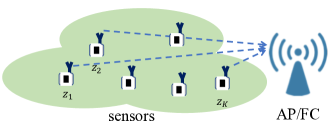
Figure 1: A WSN with multiple sensor nodes and an AP for distributed detection.

For example, suppose that the $z_{k}$’s follow a Gaussian distribution with mean vector ${\bf m}_{q}$ and covariance matrix ${\bf R}_{q}$ under hypothesis $\theta_{q}$. In this case, (1) can be re-written as

$$q^{*} =\operatorname*{\arg\!\max}_{q}\ln f({\bf z}\,|\,\theta_{q})$$ (2)

$$=\operatorname*{\arg\!\min}_{q}({\bf z}-{\bf m}_{q})^{\rm T}{\bf R}_{q}^{-1}({\bf z}-{\bf m}_{q})+\ln\det({\bf R}_{q}),$$ (3)

where ${\bf z}=[z_{1}\ \ldots z_{K}]^{\rm T}$ that is referred to as the complete information.

For a large number of sensor nodes, $K$, while a reliable decision can be made if all the measurements are uploaded to the AP, the time to receive all the measurements can be long due to a limited bandwidth, which results in a long decision delay. In particular, if only one sensor node is allowed to transmit at a slot time (in time division multiple access (TDMA)), the time to make a decision is equivalent to that to receive all the measurements, i.e., $K$-slot time (under the assumption that the processing time to choose a hypothesis according to (3) is negligible). As a result, in order to shorten the decision delay, a fraction of measurements can be used at the cost of degraded decision performance.

III Data-aided Sensing

In this section, we briefly present the notion of DAS for joint sensing and communication to efficiently upload measurements of nodes [12] [15].

Suppose that only one node can upload its measurement at each round. Denote by ${\cal Z}(l)$ the set of local measurements that are available at the AP after iteration $l$. Then, for a certain objective function, denoted by $\Theta(\cdot)$, the AP can decide the next node to upload its local information as follows:

$$k(l+1)=\operatorname*{\arg\!\min}_{k\in{\cal K}^{c}(l)}\Theta(z_{k},{\cal Z}(l)),$$ (4)

where $k(l)$ is the index of the node that is to upload its local measurement at round $l$, ${\cal K}(l)$ represents the index set of the nodes associated with ${\cal Z}(l)$, and ${\cal K}^{c}(l)$ denotes the complement of ${\cal K}(l)$. Clearly, it can be shown that ${\cal K}(l)=\{k(1),\ldots,k(l)\}$. In (4), we can see that the selected node, say $k(l+1)$, at each round depends on the accumulated measurements from the previous rounds, ${\cal Z}(l)$, which shows the key idea of DAS.

The objective function in (4) varies depending on the application. As an example, let us consider an entropy-based DAS where the AP is to choose the uploading order based on the entropy of measurements. Since ${\cal Z}(l)$ is available at the AP after iteration $l$, the entropy or information of the remained measurements becomes ${\sf H}({\cal Z}^{c}(l)\,|\,{\cal Z}(l))$, where ${\sf H}(X|Y)$ represents the conditional entropy of $X$ for given $Y$. Thus, as in [15], the following objective function can be used for the node selection:

$$\Theta(z_{k},{\cal Z}(l))=\underbrace{{\sf H}({\cal Z}^{c}(l)\,|\,{\cal Z}(l))}_{\rm Remained\ Information}-\underbrace{{\sf H}(z_{k}\,|\,{\cal Z}(l))}_{\rm Updated\ Information},$$ (5)

which is the entropy gap, where ${\sf H}(z_{k}\,|\,{\cal Z}(l))$ is the amount of information by uploading the measurement from node $k$. Clearly, for fast data collection (or data collection with a small number of nodes), we want to choose the next nodes to minimize the entropy gap.

Note that ${\sf H}({\cal Z}^{c}(l)\,|\,{\cal Z}(l))$ is independent of $k$. Thus, the next node is to be chosen according to the maximization of conditional entropy is given by

$$k(l+1)=\operatorname*{\arg\!\max}_{k\in{\cal K}^{c}(l)}{\sf H}(z_{k}\,|\,{\cal Z}(l)).$$ (6)

That is, the next node should have the maximum amount of information (in terms of the conditional entropy) given that ${\cal Z}(l)$ is already available at the AP.

In [12], the mean squared error (MSE) between the total measurement ${\bf z}$ and its estimate is to be minimized in choosing the node at round $l+1$, i.e.,

$$\Theta(z_{k},{\cal Z}(l))={\mathbb{E}}\left[||{\bf z}-\hat{\bf z}(z_{k},{\cal Z}(l))||^{2}\,|\,{\cal Z}(l)\right],$$ (7)

where $\hat{\bf z}(z_{k},{\cal Z}(l))$ is the minimum MSE estimator of ${\bf z}$ for given $\{z_{k},{\cal Z}(l)\}$ and the expectation is carried out over ${\cal Z}^{c}(l)$, which is the subset of measurements that are not available before round $l$. Since the measurements are assumed to be Gaussian in [12], second order statistics can be used for DAS, which is called Gaussian DAS. After some manipulations, it can also be shown that

$$\Theta(z_{k},{\cal Z}(l))=-{\mathbb{E}}\left[|z_{k}-\hat{z}_{k}|^{2}\,\bigl{|}\,{\cal Z}(l)\right]+C,$$ (8)

where $C$ is constant and $\hat{z}_{k}={\mathbb{E}}[z_{k}\,|\,{\cal Z}(l)]$ is the conditional mean of $z_{k}$ for given ${\cal Z}(l)$. Thus, the next node can be selected as follows:

$$k(l+1)=\operatorname*{\arg\!\max}_{k\in{\cal K}^{c}(l)}{\mathbb{E}}\left[|z_{k}-\hat{z}_{k}|^{2}\,\bigl{|}\,{\cal Z}(l)\right].$$ (9)

For Gaussian measurements, the MSE, ${\mathbb{E}}\left[|z_{k}-\hat{z}_{k}|^{2}\,\bigl{|}\,{\cal Z}(l)\right]$, is proportional to the conditional entropy, ${\sf H}(z_{k}\,|\,{\cal Z}(l))$. Thus, Gaussian DAS is also to minimize the entropy gap in selecting nodes, i.e., Gaussian DAS is also the entropy-based DAS.

IV Node Selection in Distributed Detection with DAS

In this section, we apply DAS to distributed detection. We first consider the entropy-based DAS to decide the next node in distributed detection. Then, another approach is proposed, which has the objective function based on the J-divergence.

IV-A Entropy-based DAS for Node Selection

Since the entropy-based DAS can allow the AP to estimate or approximate the complete information, ${\bf z}$, with a small number of measurements, it can be used in distributed detection. That is, under each hypothesis, the AP can collect a subset of measurements and use them to make a decision.

Suppose that the AP has a subset of measurements, i.e., ${\cal Z}(l)$, at the end of round $l$. The AP has the likelihood function, $f({\cal Z}(l)\,|\,\theta_{q})$. Under hypothesis $\theta_{q}$, the updated likelihood function with a new measurement from node $k$ becomes $f(z_{k},{\cal Z}(l)\,|\,\theta_{q})$, where $k\in{\cal K}^{c}(l)$. As in Section III, for each hypothesis $\theta_{q}$, the node selection can be carried out to minimize the entropy gap. Thus, if the ascending order is employed, the node selection becomes

$$k(Qi+q)=\operatorname*{\arg\!\max}_{k\in{\cal K}^{c}(Qi+q-1)}{\sf H}(z_{k}\,|\,{\cal Z}(Qi+q-1),\theta_{q}),$$ (10)

for $q=1,\ldots,Q$, where $Q$ nodes are selected at each $i\in\{0,1,\ldots\}$. Clearly, we have ${\cal K}(Q(i+1))={\cal K}(Qi)\cup\{k(Qi+1,\ldots,k(Q(i+1))\}$, and a decision can be made every $i$, i.e., after $Q$ nodes upload their measurements.

Alternatively, if there are $Q$ parallel channels, the selected nodes can be given by

$$k_{q}(l+1)=\operatorname*{\arg\!\max}_{k\in{\cal K}^{c}(l)}{\sf H}(z_{k}\,|\,{\cal Z}(l),\theta_{q}),\ q=1,\ldots,Q.$$ (11)

IV-B KL Divergence for Node Selection

With known measurements at the end of round $l$, i.e., ${\cal Z}(l)$, the AP can choose the next node to increase the log-likelihood ratio (LLR) for the maximum likelihood (ML) detection. For example, suppose that $Q=2$. Then, with a new measurement, the LLR is given by

$${\rm LLR}_{1,2}(z_{k},{\cal Z}(l))=\ln\frac{f(z_{k},{\cal Z}(l)\,|\,\theta_{1})}{f(z_{k},{\cal Z}(l)\,|\,\theta_{2})},\ k\in{\cal K}^{c}(l).$$ (12)

Since $z_{k}\in{\cal K}^{c}(l)$ is unknown, the expectation of LLR can be considered. Under $\theta_{1}$, the expectation of LLR is given by

$${\mathbb{E}}[{\rm LLR}_{1,2}(z_{k},{\cal Z}(l))\,|\,{\cal Z}(l),\theta_{1}],$$ (13)

and $z_{k}$ can be chosen to maximize the expectation. However, since there is also hypothesis $\theta_{2}$, for uniform prior, the objective function to be maximized can be defined as

$$\Theta(z_{k},{\cal Z}(l)) ={\mathbb{E}}[{\rm LLR}_{1,2}(z_{k},{\cal Z}(l))\,|\,{\cal Z}(l),\theta_{1}]$$ (14)

$$\quad+{\mathbb{E}}[{\rm LLR}_{2,1}(z_{k},{\cal Z}(l))\,|\,{\cal Z}(l),\theta_{2}]$$ (15)

$$={\sf D}(f_{1}(z_{k}\,|\,{\cal Z}(l))||f_{2}(z_{k}\,|\,{\cal Z}(l)))$$ (16)

$$\quad+{\sf D}(f_{2}(z_{k}\,|\,{\cal Z}(l))||f_{1}(z_{k}\,|\,{\cal Z}(l))),$$ (17)

where $f_{q}(z_{k}\,|\,{\cal Z}(l))=f(z_{k}\,|\,{\cal Z}(l),\theta_{q})$ and ${\sf D}(f(z)||g(z))={\mathbb{E}}_{f}\left[\ln\frac{f(Z)}{g(Z)}\right]$ is the Kullback–Leibler (KL) divergence between two distributions, $f(z)$ and $g(z)$ [14]. Here, ${\mathbb{E}}_{f}[\cdot]$ represents the expectation over $f(z)$. In (17), the objective function is the $J$-divergence [14] between $f_{1}(z_{k}\,|\,{\cal Z}(l))$ and $f_{2}(z_{k}\,|\,{\cal Z}(l))$.

In general, for $Q$ hypotheses, the node selection can be generalized as follows:

$$k(l+1)=\operatorname*{\arg\!\max}_{k\in{\cal K}^{c}(l)}\sum_{q=1}^{Q}\sum_{i\neq q}{\sf D}(f_{q}(z_{k})||f_{i}(z_{k})).$$ (18)

The resulting DAS that uses the node selection criterion in (18) is referred to as the J-divergence based DAS (J-DAS).

We now derive more explicit expressions for the objective function in (17) when $\{z_{k}\}$ are jointly Gaussian. For simplicity, consider $Q=2$. Then, the objective function in (17) becomes

$${\sf D}(f_{1}||f_{2})+{\sf D}(f_{2}||f_{1}) ={\mathbb{E}}_{1}[\ln f_{1}]-{\mathbb{E}}_{2}[\ln f_{1}]$$ (19)

$$\quad+{\mathbb{E}}_{2}[\ln f_{2}]-{\mathbb{E}}_{1}[\ln f_{2}],$$ (20)

where $f_{q}=f_{q}(z_{k}\,|\,{\cal Z}(l))$ and ${\mathbb{E}}_{q}[\cdot]={\mathbb{E}}_{f_{q}}[\cdot]$ for notational convenience.

For convenience, let ${\bf z}(l)$ be the column vector consisting of the elements of ${\cal Z}(l)$. In addition, let $\bar{z}_{k;q}={\mathbb{E}}_{q}[z_{k}]$, $\bar{\bf z}_{q}(l)={\mathbb{E}}_{q}[{\bf z}(l)]$, and ${\bf R}_{q}(l)={\mathbb{E}}_{q}[\left({\bf z}(l)-\bar{\bf z}_{q}(l)\right)\left({\bf z}(l)-\bar{\bf z}_{q}(l)\right)^{\rm T}]$. Let $r_{k;q}={\mathbb{E}}_{q}[(z_{k}-\bar{z}_{k;q})^{2}]$ and ${\bf c}_{k;q}(l)={\mathbb{E}}_{q}\left[\left({\bf z}(l)-\bar{\bf z}_{q}(l)\right)(z_{k}-\bar{z}_{k;q})\right]$, where $\bar{z}_{k;q}={\mathbb{E}}_{q}[z_{k}]$. Then, under $\theta_{q}$, we have

$$\left[\begin{array}[]{c}z_{k}\cr{\bf z}(l)\cr\end{array}\right]\sim{\cal N}\left(\left[\begin{array}[]{c}\bar{z}_{k;q}\cr\bar{\bf z}_{q}(l)\cr\end{array}\right],\left[\begin{array}[]{cc}r_{k;q}&{\bf c}_{k;q}^{\rm T}(l)\cr{\bf c}_{k;q}(l)&{\bf R}_{q}(l)\cr\end{array}\right]\right).$$ (21)

After some manipulations using the matrix inversion lemma [16], it can be shown that

$${\mathbb{E}}_{1}[\ln f_{1}]-{\mathbb{E}}_{2}[\ln f_{1}] =-\frac{\alpha_{k;1}}{2}\left(r_{k;1}-r_{k;2}-\bar{d}_{k}^{2}\right)$$ (22)

$$\quad-\bar{d}_{k}({\bf z}(l)-\bar{\bf z}_{1}(l))^{\rm T}{\bf b}_{k;1},$$ (23)

where $\bar{d}_{k}=\bar{z}_{k;1}-\bar{z}_{k;2}$ and

$$\alpha_{k;q} =\frac{1}{r_{k;1}-{\bf c}_{k;q}^{\rm T}(l){\bf R}_{q}^{-1}(l){\bf c}_{k;q}(l)}$$ (24)

$${\bf b}_{k;q} =-\alpha_{k;q}{\bf R}_{q}^{-1}(l){\bf c}_{k;q}(l).$$ (25)

The second term in (20), i.e., ${\mathbb{E}}_{2}[\ln f_{2}]-{\mathbb{E}}_{1}[\ln f_{2}]$, can also be found by a similar way.

For Gaussian measurements, the complexity of J-DAS mainly depends on the complexity to find the J-divergence or (23). At round $l+1$, since ${\bf z}(l)-\bar{\bf z}_{1}(l)$ is the common term for all $k\in{\cal K}^{c}(l)$, the complexity is mainly due to that to find ${\bf b}_{k;q}$ in (25). Again, ${\bf R}_{q}(l)$ is independent of $k$, the complexity to find ${\bf b}_{k;q}$ is $O(l^{2})$, while the complexity to find the inverse of ${\bf R}_{q}(l)$ from the results in the previous round is $O(l^{2})$. Thus, the complexity at round $l+1$ is $O((K-l)l^{2})$. Thus, if the number of iterations is $T(\ll K)$, the total complexity is bounded by $O(K\sum_{l=1}^{T}l^{2})=O(KT^{3})$.

V Simulation Results

In this section, we present simulation results with LLRs. For each average LLR, the results of 500 independent runs are used. In simulations, we assume that the $z_{k}$’s are jointly Gaussian with $K=50$ and $Q=2$. For comparisons, we consider the three node selection criteria: J-DAS (i.e., (18)), entropy-based DAS (i.e., (10)), and random selection.

For the first simulation, we assume that

$$\bar{z}_{k;1}=A\cos\left(\frac{\pi}{10}(k-1)\right),\ \bar{z}_{k;2}=A\sin\left(\frac{\pi}{10}(k-1)\right),$$ (26)

where $A>0$ is the amplitude of the mean signal. In addition, the covariance matrix of ${\bf z}$ under $\theta_{q}$ is given by

$$[{\bf R}_{q}]_{k,t}=\sigma^{2}(\rho_{q})^{|k-t|},\ k,t=1,\ldots,K,$$ (27)

where $\rho_{1}=\frac{3}{4}$ and $\rho_{2}=-\frac{3}{4}$, and $\sigma^{2}$ represents the noise variance. The signal-to-noise ratio (SNR) is defined as ${\sf SNR}=\frac{A^{2}}{2\sigma^{2}}$. In Fig. 2, the average LLR is shown as a function of iterations. When $\theta_{1}$ is correct, it is shown that the LLR increases with the number of samples or iterations. Clearly, the performance of J-DAS outperforms those of entropy-based DAS and random selection. In other words, when a decision is made with a small number of iterations or samples in distributed detection, J-DAS can help provide reliable outcomes compared to the others.

It is interesting to see that the entropy-based DAS does not provide a good performance in distributed detection as shown in Fig. 2. The entropy-based DAS is to choose the node that has the most uncorrelated measurement as shown in (10). In fact, such a measurement needs not contribute to maximizing the difference between the hypotheses.

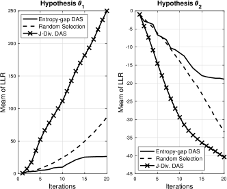
(a)                               (b)

Figure 2: The sample mean of LLR when the $z_{k}$’s are jointly Gaussian when the means and covariance matrices are given by (26) and (27), respectively, with ${\sf SNR}=0$ dB and $K=50$: (a) when $\theta_{1}$ is true; (b) when $\theta_{2}$ is true.

For the next simulation, we consider the case of iid measurements. That is, ${\bf R}_{q}=\sigma^{2}{\bf I}$ for all $q\in\{1,2\}$. In addition, it is assumed that $\bar{z}_{k;1}=A$ and $\bar{z}_{k;2}=-A$ for all $k$. As mentioned earlier, in this case, the performance is independent of the uploading order, which can be confirmed by the results in Fig. 3.

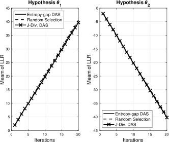
(a)                               (b)

Figure 3: The sample mean of LLR when the $z_{k}$’s are iid Gaussian with ${\sf SNR}=0$ dB and $K=50$: (a) when $\theta_{1}$ is true; (b) when $\theta_{2}$ is true.

VI Concluding Remarks

In this paper, the notion of DAS has been exploited to provide a good performance of distributed detection in WSN with a smaller number of sensors that upload their measurements. In particular, a J-divergence based node selection criterion was proposed for DAS, which was referred to as J-DAS, so that the measurement from the next node can maximize LLR. From simulation results, it was shown that LLR increased rapidly as the number of iterations increased when J-DAS was employed.

There would be a number of further research topics. Among those, as in [17], the application of J-DAS to distributed machine learning for classification is interesting. The performance analysis of J-DAS would also be another topic to be studied in the future.

References

- [1] W. Dargie and C. Poellabauer, Fundamentals of Wireless Sensor Networks: Theory and Practice. Wiley Publishing, 2010.
- [2] Q. Zhu, R. Wang, Q. Chen, Y. Liu, and W. Qin, “IOT gateway: Bridging wireless sensor networks into Internet of Things,” in 2010 IEEE/IFIP International Conference on Embedded and Ubiquitous Computing, pp. 347–352, 2010.
- [3] Y. Kuo, C. Li, J. Jhang, and S. Lin, “Design of a wireless sensor network-based IoT platform for wide area and heterogeneous applications,” IEEE Sensors Journal, vol. 18, pp. 5187–5197, June 2018.
- [4] P. K. Varshney, Distributed Detection and Data Fusion. New York: Springer, 1997.
- [5] R. Viswanathan and P. Varshney, “Distributed detection with multiple sensors i. fundamentals,” Proceedings of the IEEE, vol. 85, no. 1, pp. 54–63, 1997.
- [6] J.-F. Chamberland and V. V. Veeravalli, “Decentralized detection in sensor networks,” IEEE Trans. Signal Process., vol. 51, pp. 407–416, feb 2003.
- [7] B. Chen, L. Tong, and P. K. Varshney, “Channel-aware distributed detection in wireless sensor networks,” IEEE Signal Process. Mag., vol. 23, pp. 16–26, jul 2006.
- [8] S. He, J. Chen, D. K. Y. Yau, and Y. Sun, “Cross-layer optimization of correlated data gathering in wireless sensor networks,” in 2010 7th Annual IEEE Communications Society Conference on Sensor, Mesh and Ad Hoc Communications and Networks (SECON), pp. 1–9, June 2010.
- [9] A. Chawla, A. Patel, A. K. Jagannatham, and P. K. Varshney, “Distributed detection in massive MIMO wireless sensor networks under perfect and imperfect CSI,” IEEE Trans. Signal Processing, vol. 67, no. 15, pp. 4055–4068, 2019.
- [10] T. L. Marzetta, “Noncooperative cellular wireless with unlimited numbers of base station antennas,” IEEE Trans. Wireless Communications, vol. 9, pp. 3590–3600, Nov. 2010.
- [11] J. Choi, “A cross-layer approach to data-aided sensing using compressive random access,” IEEE Internet of Things J., vol. 6, pp. 7093–7102, Aug 2019.
- [12] J. Choi, “Gaussian data-aided sensing with multichannel random access and model selection,” IEEE Internet of Things J., vol. 7, no. 3, pp. 2412–2420, 2020.
- [13] A. Wald, “Sequential tests of statistical hypotheses,” Ann. Math. Statist., vol. 16, pp. 117–186, 06 1945.
- [14] S. Kullback, Information Theory and Statistics. New York: Wiley, 1959.
- [15] J. Choi, “Data-aided sensing where communication and sensing meet: An introduction,” in 2020 IEEE Wireless Communications and Networking Conference Workshops (WCNCW), pp. 1–6, 2020.
- [16] D. A. Harville, Matrix Algebra From a Statistician’s Perspective. New York: Springer, 1997.
- [17] J. Choi and S. R. Pokhrel, “Federated learning with multichannel ALOHA,” IEEE Wireless Communications Letters, vol. 9, no. 4, pp. 499–502, 2020.