Abstract

Forecasting the number of trips in bike-sharing systems and its volatility over time is crucial for planning and optimizing such systems. This paper develops timeseries models to forecast hourly count timeseries data, and estimate its volatility. Such models need to take into account the complex patterns over various temporal scales including hourly, daily, weekly and annual as well as the temporal correlation. To capture this complex structure, a large number of parameters are needed. Here a structural model selection approach is utilized to choose the parameters. This method explores the parameter space for a group of covariates at each step. These groups of covariate are constructed to represent a particular structure in the model. The statistical models utilized are extensions of Generalized Linear Models to timeseries data. One challenge in using such models is the explosive behavior of the simulated values. To address this issue, we develop a technique which relies on damping the simulated value, if it falls outside of an admissible interval. The admissible interval is defined using measures of variability of the left and right tails. A new definition of outliers is proposed based on these variability measures. This new definition is shown to be useful in the context of asymmetric distributions.

Keywords: Stochastic Processes; Count Time Series; Volatility; Model Selection; Bike-sharing; Grouped Structural Model Selection

1 Introduction

Bike-sharing systems are being developed in many urban areas as a low cost technology to solve mobility of millions of people. These systems have access to rich data over time, since the timestamp of each check-in and check-out are collected automatically. These data can be used to calculate the number of trips in any time-interval, in a certain area or the number of trips between any two areas in the city. The methods discussed in this paper apply to other ride-sharing systems using cars (e.g. Uber, Lyft) and public transit.

The focus of this paper is to develop models to estimate the number of trips at any given time. We also require the models to estimate the remaining volatility of the series – not explained by seasonality and long-term trends. Some applications of these models are (a) short-term and long-term planning for the demand in the system; (b) investigating the impact of interruptions in the system; (c) planning for re-balancing of the bikes throughout the system; (d) anomaly detection, e.g. for detecting events in the city and labeling them as discussed in Fanaee et al. (2013).

The contributions of this paper are as follows. From an application point of view, most of the work in this area (ride-sharing) are focused on forecasting the number of trips in short-term (in the order of a few days/weeks into the future) using machine learning algorithms without an explicit model for volatility e.g. Fanaee et al. (2013) and Yang et al. (2016). Here, we provide long-term forecasts and more importantly accurate estimates of the volatility of the series over time.

From a methodological point of view, a comprehensive summary of previous work can be found in Fokianos (2012), which classifies the methods into two categories: (1) Regression Timeseries Methods (e.g. Kedem et al. (2002)); (2) Integer Autoregressive Models (e.g Nastic et al. (2012)). This work uses (1), because it can explicitly model complex temporal variations in the series as shown in Hosseini et al. (2015a) for Gaussian series with time-varying variance or in Hosseini et al. (2017) for non-negative valued timeseries (e.g. precipitation). The statistical timeseries models utilized in this paper are based on extensions of Generalized Linear Models to timeseries context (e.g. Kedem et al. (2002), Hosseini et al. (2015a)). In order to apply these models, one challenge is the complexity of the temporal trends in various scales: daily, weekly and annual and the large number of lags needed to capture the time-dependence. Modeling these features require a large number of parameters, which can cause over-fitting and instability in the models. The issue of over-fitting is extensively discussed in the machine learning context and statistics (e.g. Hastie et al. (2009)). Various model selection techniques have been developed to solve this problem. There are three main techniques to avoid over-fitting (1) cross-validation methods (see Hastie et al. (2009)); (2) methods which penalize the complexity of the model; (e.g. AIC, Akaike (1974) or BIC, Schwartz (1978)) (3) regularization methods such as Ridge Regression and Lasso (see Hastie et al. (2009)). The method utilized here is called Grouped Structural Model Selection (GSMS) and it falls under (2). At each step of GSMS, rather than considering one variable, a group of variables – which represent a particular structure of the series – is considered. This is the first application of this method to count time-series data and at the hourly granularity.

While model selection helps with the stability of the model and allows us to fit very complex patterns, an additional fundamental complexity needs to be addressed to ensure: the simulated long-term future series do not diverge (produce unrealistic values, which are very far from historical values). Tong (1990) and Hosseini et al. (2015a) discuss methods to avoid this issue in the context of non-linear Gaussian series and in Hosseini et al. (2017) in the context of Bernouli-Gamma series for precipitation modeling. For simplicity, assume $Y(t)=f(t)+\epsilon(t),$ where $f(t)$ is a complex function of previous lags (e.g. includes $Y(t-1)$) and $\epsilon(t)$ is a noise process. To avoid this potential explosive behavior, Tong (1990) suggested hard or soft censoring of $f(t)$ by replacing it with $f(t)1_{(-a,a)}(f(t))$ which sets $f(t)$ to zero if it goes beyond the interval $(-a,a)$ for some positive value of $a$. Hosseini et al. (2015a) used a damping approach by setting back $Y(t)$ to $M$ if $Y(t)>M$ and to $m$ if $Y(t)<m$ for some appropriate real numbers $m<M$ chosen based on historical observations. However, for some data sets and models, this is not sufficient and we suggest a method which lets $m$ and $M$ to depend on some notion of seasonality. Moreover, in order to find an upper bound ($M$) and lower bound ($m$), we present a new definition of outliers. This definition allows for the lower and upper bounds to use their own notion of variability depending on the left and right tails of the distribution of the data.

The paper is organized as follows. Section 2 performs an exploratory analysis of the data. Section 3 discusses the underlying statistical models. Section 4 discusses the model selection procedure. Section 5 develops a damping procedure for the simulated values to insure the simulated values do not diverge. This method allows for the damping parameters to depend on time. To decide the upper bound and lower bounds for the damping, we introduce an asymmetric definition of outliers which can be useful in many other applications. Section 6 discusses the results of the model selection and damping procedure for the bike-sharing data. Section 7 provides a summary and discussion of the methods in this paper. Appendix A includes comparison with a variety of other related models to the main text.

2 Exploratory analysis

The dataset in this work includes the hourly counts of rented bikes in Washington DC during 2011 and 2018 and were obtained from www.capitalbikeshare.com.

The raw hourly count data are shown in the Top Left Panel of Figure 1. The annual average count (per hour) curve is given in the Top Right Panel, showing an increasing long-term trend. The Bottom Left Panel depicts the weekly average counts (per hour) and again showing a year long seasonal pattern with largest counts during the warm season. The Bottom Right Panel shows the average and the standard deviation of hourly count with respect to the time of the week, starting from 0 (denoting Sunday 00:00 am), to 7 (denoting 24:00 on Saturday). We observe a very strong weekly pattern in the average and variance measures.

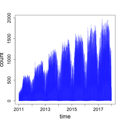
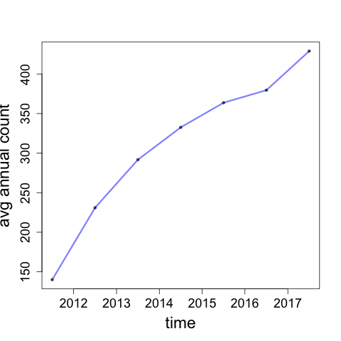
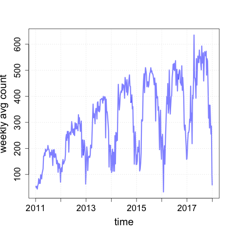
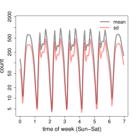
Figure 1: Top Left Panel: observed hourly count over time; Top Right Panel: annual average count (per hour); Bottom Left Panel: long-term weekly average count (per hour); Bottom Right Panel: observed mean and standard deviation with respect to the time of week.

3 Statistical models

Suppose $\{Y(t)\},t=0,1,\cdots$ is a count process, where $t$ denotes time. We denote the available information up to time $t$ by $\mathcal{F}(t-1)$. We assume this information is given in terms of a covariate process, denoted by ${\bf Z}(t)$, as discussed in Kedem et al. (2002). For example, we can consider the covariate process:

$${\bf Z}(t-1)=(1,Y(t-1),Y(t-2),f_{d}(t),f_{w}(t),f_{y}(t)),$$

where $,f_{d}(t),f_{w}(t),f_{y}(t)$ are each a vector of periodic functions over: a day period; a week period; and a year period, respectively.

An example for $f_{d}$ is the following vector of terms of a Fourier series:

$$f_{d}(t)=\big{(}\sin(\omega_{d}t),\cos(\omega_{d}t)\big{)},$$

where $\omega_{d}=2\pi/24$ is the time frequency. This means the above function is periodic with periodicity of 24, which is appropriate for hourly data.

We further assume, a linear form for the transformed conditional mean:

$$g(\mathop{{}\mathbb{E}}\{Y(t)|\mathcal{F}(t-1)\}) ={\bf\beta}{\bf Z}(t-1),$$ (1)

where $g$ is the transformation, also referred to as: the link function.

We assume, the conditional distribution of $Y(t)$ belongs to the Exponential Family and has one of the following forms:

• Poisson distribution, with density function:

  $$f_{Y}(y)={\frac{\lambda^{y}}{y!}}e^{-\lambda},\;\;y=0,1,2,\cdots,$$

  where $\lambda=\mathop{{}\mathbb{E}}(Y)=\text{Var}(Y).$ In this case $\text{Var}(Y)/\mathop{{}\mathbb{E}}(Y)=1.$

• Negative Binomial distribution, with density function:

  $$\Pr(Y=y)={\frac{\Gamma(\theta+y)}{y!\,\Gamma(\theta)}}\left({\frac{\mu}{\theta+\mu}}\right)^{y}\left({\frac{\theta}{\theta+\mu}}\right)^{\theta}\quad{\text{for }}y=0,1,2,\dotsc$$

  where $\mathop{{}\mathbb{E}}(Y)=\mu$ and $\text{Var}(Y)=\mu+\mu^{2}/\theta.$ Therefore, we have $\text{Var}(Y)/\mathop{{}\mathbb{E}}(Y)=1+\mu/\theta$ which increases as $\mu$ increases.

For the Poisson distribution, the property: $\mathop{{}\mathbb{E}}(Y)=\text{Var}(Y),$ seems very limiting at first. In fact, many authors report over-dispersion in real data, in the context of Poisson regression (e.g. Thall and Veil (1990), Berk and MacDonald (2008) and Zheng et al (2006)). However, the above model is a conditional Poisson distribution of the form: $\mathop{{}\mathbb{E}}\{Y(t)|\mathcal{F}(t-1)\})$. This means, the conditional distribution, (potentially conditioned on a complex ${\bf Z}(t-1)$), is distributed as a Poisson. In fact, we are not assuming, the marginal distribution of $Y(t)$ is Poisson. In particular, note that, if the covariate process: ${\bf Z}(t-1)$, includes complex seasonality components, growth components and lags (as suggested above), some extra variability will be induced in the series, which might (or might not) be sufficient to capture the true variability in the series. In order to check for that, we compare the variability observed in the model-based simulations to the observed variability on a validation set.

The Negative Binomial Model has an extra parameter, which allows the variability to increase, as the conditional mean increases. Therefore, it can accommodate more over-dispersion than the Poisson Model. In this work, we consider both Poisson and Negative Binomial for a variety of models with complex conditional means and compare the results. It turns out that, with sufficiently complex conditional mean structures, even the Poisson model is able to capture the time-varying volatility well.

Other related models considered in the literature include the Quasi-Poisson Regression Model. For example, Ver Hoef and Boveng (2007) compares the performance of Quasi-Poisson and Negative Binomial regression models to capture the over-dispersion. One issue with using Quasi-Poisson models is the lack of a distribution function to simulate from. One idea is to use the estimated model’s mean and variance for the quasi-likelihood, and pick a distribution with matching mean and variance (for example Gaussian, Gamma, or Poisson). We tested this approach in this work, and the results were generally inferior to Negative Binomial and Poisson. Therefore, we do not present them for brevity. Another distribution proposed to capture the over-dispersion is the Double Poisson distribution introduced by Efron (1986). This distribution is suggested to capture the over-dispersion in the timeseries context in Heinen (2003).

4 Model selection

Let $\{Y(t)\},t=0,1,\cdots$, denote the hourly count data observed over time. Then each time has these associated values:

• time of day (shorthand: tod) (in hours) which we denote by $d(t)$ ranging from 0 to 23;

• time of week (shorthand: tow) ranging from 0 to 6 which we denote by $w(t)$ (with 0 denoting Sunday);

• time of year (shorthand: toy) which ranges from 0 to 365 (or 366) which we denote by $a(t)$.

We allow these variables to change in the smallest scale available in the data. For example for noon of Monday Jan 15th we have:

$$d(t)=12,w(t)=1.5,a(t)=14.5.$$

To capture the daily patterns, we use a Fourier terms of the form:

$$s_{k}(t)=\sin(k\omega_{d}d(t)),\;c_{k}(t)=\cos(k\omega_{d}d(t)),\;\omega_{d}=2\pi/24,$$

$$k=1,\cdots,K_{1}$$

In order to allow for contrast between weekends and weekdays, we introduce similar terms which are equal to the above over the weekends and zero otherwise:

$$\begin{cases}s_{k}^{\prime}(t)=s_{k}(t),\;c_{k}^{\prime}(t)=c_{k}(t),&\mbox{t in weekend}\\ s_{k}^{\prime}(t)=0,\;c_{k}^{\prime}(t)=0,&\mbox{otherwise}\end{cases}$$

$$k=1,\cdots,K_{2}$$

To allow extra day-to-day variation between weekdays, we introduce weekly Fourier series terms:

$$s_{k}^{w}(t)=\sin(k\omega_{w}w(t)),\;c_{k}^{w}(t)=\cos(k\omega_{w}w(t)),\;\omega_{w}=2\pi/7.$$

$$k=1,\cdots,K_{3}$$

We also showed a seasonal effect throughout the year (Figure 1), which we capture by introducing

$$s_{k}^{a}(t)=\sin(k\omega_{a}a(t)),\;c_{k}^{a}=\cos(k\omega_{a}a(t)),$$

$$\omega_{a}=2\pi/365,\;\omega_{a}=2\pi/366\;(\mbox{for leap years}).$$

$$k=1,\cdots,K_{4}$$

To capture the temporal correlation, we consider the lags: $Y(t-1),Y(t-2),\cdots$. To capture long-term dependence in the series, without using a large number of lags, we consider the long-term average lag processes:

$$av_{j}(t)=\sum_{i=1}^{j}Y(t-i)/j,$$

introduced in Hosseini et al. (2011b) and R. Hosseini et al. (2012) for modeling precipitation and frost occurrence respectively. For example, $av_{5}$ is the average of the past 5 time-periods (hours in for our data) and $av_{24}$ is the average amount over the past 24 hours.

One issue with using lags in the model, especially when the link function ($g$ in Equation 1) is the $log$ function is, more chance of explosive behavior of the simulations. One technique to decrease this chance is to use transformations of the lags as discussed in Fokianos (2012). Here, we observed that using appropriate lag transformations indeed decreased the chance of explosive behaviors and used this lag transformation:

$$f(y(t-i))=\log(0.1+y(t-i)).$$

The constant 0.1 is added to prevent $f$ from being undefined at zero. We recommend using a constant between (0.1, 1) here so that 0 is mapped to a value between (-1, 0). Note that using a very small value e.g.  0.0001 maps 0 to -4 and the model might get stretched too far to fit the 0 values, while in this context the difference between 0 counts and small counts is not significant in practice. In the main text, we present the results with lag transformations and in the appendix, we show the undesirable impact of removing the lag transformations from the model.

To capture the long-term trends/growth of the series, as suggested by the Top Right Panel of Figure 1, we use $t$ and its powers e.g. $t,t^{2},t^{3},t^{1/2},t^{1/3}$ as covariate. However, we only allow one of these variables in the model (as decided by the model selection procedure), to prevent over-fitting when simulating long-term future series.

Considering the large number of parameters needed to capture the variability of the series over multiple temporal scales, an efficient model selection procedure to reduce the number of parameters is needed. Here, we utilize the Grouped Structural Model Selection (GSMS) approach proposed in Hosseini et al. (2015b) and Hosseini et al. (2015a) for estimating soil moisture and daily temperature respectively using Gaussian models. Hosseini et al. (2017) utilized this approach for modeling daily precipitation process using a conditional Bernoulli-Gamma for the occurrence and amount. This paper is the first application of this method to hourly time series data. Also this is the first application of GSMS to count data.

GSMS works by grouping the related covariates into groups, each representing a particular structure of the model, e.g. daily patterns, weekly patterns, lags etc. Then GSMS limits the search to the subsets of a group (a pre-defined set of covariates) at each stage.

Table 1 includes the proposed groups for this application with their corresponding elements (covariates). The groups $tod,tod_{wd},tow,toy$ are introduced to capture the trends in the series over various temporal scales. The groups $lags$, and $avglag$ are introduced to capture the remaining auto-correlation in the series after removing the seasonal patterns and finally the $growth$ group is there to model the long-term trends of the series over time (as a result of system expansion and population increase).

Table 1: Covariate groups considered for GSMS procedure are given in the table. Each group represents a structure in the model. For example $tod$ captures the hourly variation across the day.

Group (acronym)	Elements/Variables
time of day ($tod$)	$s_{1},c_{1},\cdots,s_{10},c_{10}$
time of day in weekend ($tod_{wd}$)	$s_{1}^{\prime},c_{1}^{\prime},\cdots,s_{10}^{\prime},c_{10}$’
time of week ($tow$)	$s_{1}^{w},c_{1}^{w},\cdots,s_{10}^{w},c_{10}^{w}$
time of year ($toy$)	$s_{1}^{a},c_{1}^{a},\cdots,s_{10}^{a},c_{10}^{a}$
lags ($lags$)	$y(t-1),\cdots,y(t-10)$
long-term averaged lags ($avglag$)	$av_{i},\;i=5,10,15,24,48$
long-term growth ($growth$)	$t,t^{2},t^{3},\sqrt{t},\sqrt[3]{t}$

Here, we briefly describe the Grouped Structural Model Selection (GSMS) method. Suppose, the predictors $S=\{z_{1},\cdots,z_{p}\}$ are chosen already; $S^{\prime}$ is another set (group) of predictors; and $crit$ is a criterion to compare models (e.g. AIC or BIC). We denote the value of the criterion for a set of predictors $S$ by $crit(S)$. The union of two sets of predictors $S,S^{\prime}$ is denoted by $(S\cup S^{\prime})$. Then, we define the optimal merge, $om,$ of $S^{\prime}$ conditioned on the predictors $S$, as follows:

$$om(S^{\prime}|S,crit)=\underset{H\subset S^{\prime}}{argmin}\;crit\{(H\cup S)\}.$$

In other words, $om$ picks the subset of $S^{\prime}$ which once added to $S$ attains the best performance according to the criterion $crit$. We use a sequential approach combined with merging for the model selection performed in this work.

Other than the grouping, we also need to specify a model selection diagram (flow) to describe how the algorithm scans through various groups. Note that mathematically the diagram is a directed graph with nodes consisting of a group of covariates to optimize and the inward edges deliver the optimal elements calculated in previous nodes.

Figure 2 shows the main model diagram in this paper, which is a fairly simple diagram. See Hosseini et al. (2015a), Hosseini et al. (2017) for more complex GSMS diagrams. In the following, we also consider other modeling diagrams which are simplifications of the main one in Figure 2. These simplifications are described in Table 2.

The advantages of using GSMS over some other model selection approaches such as stepwise regression (see e.g. Hastie et al. (2009)) are:

• GSMS allows us to divide the covariates into groups of related covariates. Each group can represent a structural component of the model and we can assess the effect of adding or omitting a structure to the model rather than a single covariate.

• We can use: (a) exploratory analysis results; (b) expert knowledge of the process; (3) and the robustness of the covariates; to decide which structures should be added to the model first. For example, from both expert knowledge and exploratory analysis, we know that daily patterns (captured by Fourier terms based on $tod$) can explain a large portion of the variability in the response and therefore we can add that structure to the model first. Also daily patterns as compared to lag terms have the advantage of being completely determined in the future and therefore are more robust. Note that, lag terms need to be filled in by simulated values when we are performing long-term forecasting. This can cause the series to start diverging to points in the input space which have not been observed, thus resulting in the model producing unreasonable values.

• The GSMS approach allows us to fix a chosen component into the model (for example, the seasonal component) and then assess if adding another structure is beneficial.

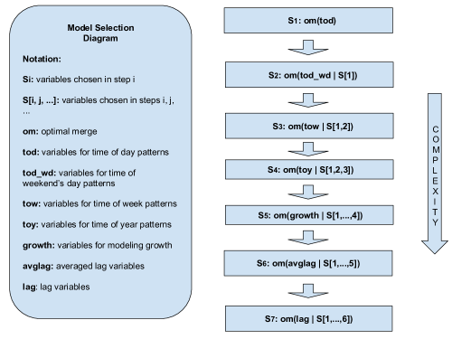
Figure 2: Model selection diagram for the bike-sharing data. In the first step ($S_{1}$), GSMS performs a search in the Fourier terms based on time of day ($tod$) and it proceeds to add patterns at other temporal scales in $S_{2},S_{3},S_{4}$. Then in $S_{5}$ it adds the long-term growth and finally in $S_{6},S_{7}$ it allows for unexplained autocorrelation using lags and their averages.

model complexity string	structure (groups)
seas_only	$(tod,tod_{wd},tow,toy)$
seas_growth	seas_only + $growth$
seas_growth_avglag	seas_only + $avglag$ + $growth$
seas_growth_lag	seas_only + $lag$ + $growth$
seas_growth_avglag_lag	seas_only + $avglag$ + $lag$ + $growth$

Table 2: Various model complexity scenarios which are compared. In the first row, seas_only is a model which only uses deterministic temporal patterns (no lags). Other rows add other structures to seas_only e.g. lags.

5 Time-varying damping

In order to forecast the future values of the series and the volatility, we simulate the future values using the fitted models. One issue with simulation in the timeseries context is the possibility of explosive behavior for complex models. This means, the simulated series is chaotic and does not look like the observed series – values far beyond what is been observed. This is generally not an issue for standard predictive models e.g. in an interpolation or classification problem. The reason for the explosive behavior in timeseries context is two fold: (1) We are simulating values as opposed to simply finding a good prediction which is the case in many machine learning application. (2) We often need to simulate a much longer period than one time ahead and as we move more into the future, the simulated values will depend on other simulated values (e.g. due to presence of lags in the model). Hence, there is more chance of gradually moving into a point in the input space (covariate space) which is not seen before (by the trained model) and this could lead in simulating unrealistic values.

The explosive behavior in simulated timeseries values was discussed by Tong (1990) and Hosseini et al. (2015a) for non-linear autoregressive Gaussian processes. In that context, we have $Y(t)=f(t)+\epsilon(t)$ where $f(t)$ is a polynomial function of previous lags and $\epsilon(t)$ is Gaussian noise with potentially time-varying variance. To avoid the explosive behavior, Tong (1990) suggested hard or soft censoring of $f(t)$ by replacing it with $f(t)1_{(-a,a)}(f(t))$ which sets $f(t)$ to zero if it goes beyond the interval $(-a,a)$ for some positive value of $a$. Hosseini et al. (2015a) used the censoring idea for the $Y(t)$ process by setting $Y(t)$ to

$$Y^{\star}(t)=\begin{cases}M,&Y(t)\geq M\\ Y(t),&m<Y(t)<M\\ m,&Y(t)\leq m\end{cases}$$

for some real numbers $m<M$, to also assure the noise process $\epsilon(t)$ does not become too large and cause explosive behavior. In this approach, $m$ and $M$ can be chosen more naturally using the historical observations.

Here, we extend the above method in two ways: (1) by allowing $(m,M)$ to vary with respect to other variables; (2) by defining a more systematic way to pick $(m,M)$ which is more reasonable for skewed and asymmetric distributions. For the bike-sharing application, we allow $m,M$ to depend on the time of the week. This is because the response variable’s volatility shows a large variability with respect to the time of the week (Figure 1).

Since we know counts cannot be negative, and we do observe small values in the data, close to zero, it is reasonable to assume $m=0$. However, in order to illustrate how the method works in general, we do not assume $m=0$.

Here, we describe a new method to define outliers, which considers the possibility of the distributions being assymetric. There are several definition of outliers in the literature, some going back to the 19th century. As an example, Chauvenet (1891) provides a definition using the mean and standard deviation of the data, based on Gaussian distribution. One of the most popular definitions of outliers is developed by John Tukey and discussed in Tukey (1977). Tukey defines a point to be an outlier, if it falls outside the interval:

$$Q_{1}-k(Q_{3}-Q_{1}),Q_{3}+k(Q_{3}-Q_{1}),$$

where $Q_{1},Q_{3}$ are the first and thrid quartiles of the data distribution and $k$ is a constant. Tukey proposed to use $k=1.5$. The difference $\delta=Q_{3}-Q_{1}$ is called the Interquantile Range (IQR). The IQR is in utilized widely in statistics going back to early 20th century (e.g. Yule (1911) and Upton (1996)). Note that the IQR measures the variability of the data in the center of the distribution – 50 percent of the data is within that range.

In order to define the outliers, first we define new quantile-based measures of data variability. The intuitive idea behind the following definitions is to measure the variability of the data on the left and right side of the distribution instead of the center – which is the case for IQR.

To that end, denote the distribution of the observed values by $D$ and let $q_{D}(p)$ denote the quantile of $D$ for $p\in[0,1]$. Note that, with this notation, the IQR is given by

$$IQR(D)=q_{D}(0.75)-q_{D}(0.25).$$

Then consider three real numbers,

$$0<p_{r},p_{l},\delta_{p}<1,$$

such that

$$0<p_{r}<p_{r}+\delta_{p}<0.5<p_{l}-\delta_{p}<p_{l}<0,$$

and require

$$p_{l}=1-p_{r}.$$

The indices $r$ and $l$ denote right and left respectively. As an example, consider

$$p_{r}=0.01,\;p_{r}+\delta_{p}=0.1,\;p_{l}-\delta_{p}=0.9,\;p_{l}=0.99.$$

See Figure 3 for a demonstration of these values and their relationship. Next, we define two measures of dispersion for the right and left tails to be

$$RTV(D) =\frac{q_{D}(p_{r}+\delta_{p})-q_{D}(p_{r})}{\delta_{p}},$$

$$LTV(D) =\frac{q_{D}(p_{l})-q_{D}(p_{l}-\delta_{p})}{\delta_{p}},$$

and we call them right and left tail-variability ($TV$) respectively. $RTV(D)$ and $LTV(D)$ can be interpreted as rate of change of quantile function in $[p_{r},p_{r}+\delta_{p}]$, and $[p_{l}-\delta,p_{l}]$ intervals respectively.

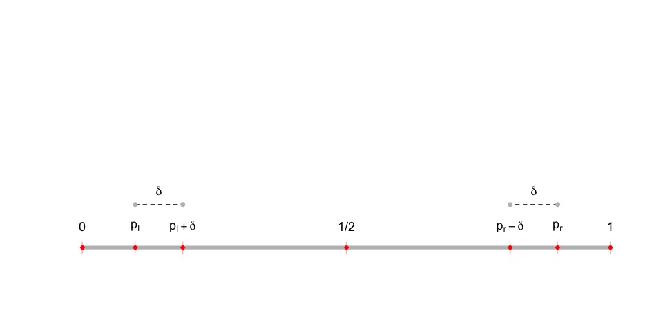
Figure 3: A demonstration of the values used in the definition of right and left tail variability given in Equation 5.

The difference between $TV$ and $IQR$ is: while $IQR$ measures the variation of data in the center of the distribution, $RTV$ and $LTV$ measure the variation of the data on the right and left sides/tails of the distribution.

Now we define the lower ($m$) and upper ($M$) limits for defining outliers:

$$m =q_{D}(p_{m})-\alpha RTV(D)$$

$$M =q_{D}(p_{M})+\alpha LTV(D),$$

$$\mbox{where }0<p_{m}\leq 1/2\leq p_{M},$$

$$\mbox{and }p_{M}=1-p_{m},\alpha\geq 0.$$

In order to contrast with Tukey’s definition, note that: $q_{D}(p_{m})$, and $q_{D}(p_{M})$ play the role of $Q_{1}$ (First Quartile) and $Q3$ (Third Quartile). Here, we further assume that $p_{m}=p_{r}$ and $p_{M}=p_{l}$ for simplicity.

We can interpret these quantities as an extension to classical definition of outliers which is useful in dealing with asymmetric distributions. In order to find a rule of thumb to choose $\alpha$, note that if hypothetically the true quantile function change approximately in the same rate as $RTV/LTV$, the minimum/maximum value attained by the distribution would be approximated by

$$q_{D}(0) \approx q_{D}(p_{m})-p_{m}RTV(D),$$ (2)

$$q_{D}(1) \approx q_{D}(p_{M})+p_{m}LTV(D).$$

Clearly, one should not expect the rate of change of the quantile function to remain constant. However this calculation gives some idea of what can be a good rule of thumb. For example if we assume the rate of change could be 10 times higher than above, we can choose $\alpha=10p_{m}$.

Note that, for a continuous distribution such as Gaussian (or other distributions with positive-valued continuous density across $\mathbb{R}$) $q_{D}(0)=-\infty$ and $q_{D}(1)=\infty$. Therefore, the above equations in (2), cannot hold. However, one can argue that in most real world applications, in fact almost no variable can have positive probability beyond a bounded interval including in our case. For example while we might assume a Poisson conditional distribution, we know that actually a value beyond $10^{9}$ bikes at any given time is impossible in one city for one hour.

For this application we choose $p_{r}=p_{m}=0.025$ an $alpha=10\times p_{m}=2.5$. Then we apply this to the observed distribution of the data for every hour of the week. The results are given in Figure 4, where the bounds $m,M$ depend on the time of the week and the obtained bounds are overlay-ed on top of the observations for comparison. We can observe that the lower bounds are closer to the historical observations since there is less variability in the low values. As discussed before, in this case we have the external information that the values can attain zero and cannot be negative, therefore a reasonable choice is $m=0$ for all $t$.

We refer to the above procedure as the Time-Varying Damping Method ($TDM$). It should be noted that, in general, models which do not require damping are preferred. In fact, based on our experience, as a rule of thumb, if a model requires more than 20% damping, one should be cautious about using the model and try to find an alternative model. In other words, $TDM$ is useful when a model generally performs well but has some chance of drifting into unrealistic values.

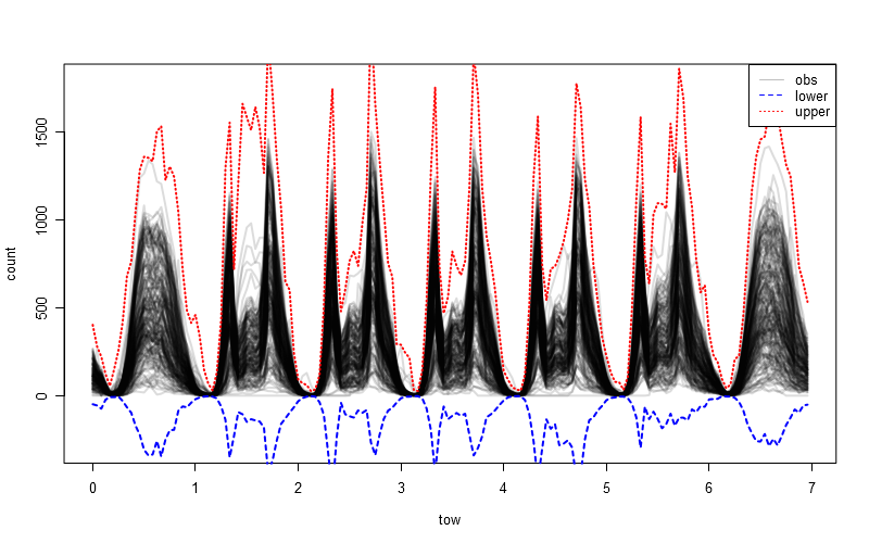
Figure 4: The obtained time-varying admissible intervals for for simulated are between the lower (denoting $m$, dashed curve) and upper bounds (denoting $M$, dotted curve) in the plot. The observed counts during 2011-2015 (training period) are also overlay-ed in the plot in transparent gray.

6 Results

The results of the model selection and simulations for models with transformed lags and with application of $TVM$ (Time-varying Damping Method) are given in Tables 3 and 4.

Table 3 contains the performance of the fit for various model complexity levels. We have standardized the AIC and BIC values by dividing them by the number of observations. In general, the models based on Negative Binomial (denoted by NB) have smaller AIC and BIC but the correlation between observed and fitted are similar across model complexity for Negative Binomial and Poisson.

The seasonal only (seas_only) model (which includes daily, weekly and annual Fourier terms) has captured 84% of the correlation already. Also as we increase the complexity, the correlation increases with non-negligible jumps when adding the growth components and either of the lag based components. However adding the groups $lags$, $avglag$ (see Table 1 for definition) or both resulted in comparable correlations.

In order to test the model performance further, we split the data to a training set which includes the observations from beginning of 2011 to end of 2015 and a test set from the beginning of 2016 to the end of 2018. The simulation results for each of the models is given in Table 4. This table reports: (i) the percent of damped simulated values; (ii) the correlation between the simulated values and the test set; (iii) the Mean Absolute Error (MAE); and (iv) Root Mean Square Error (RMSE). We observe that in general the Poisson model requires less damping as compared with the Negative Binomial model. Moreover, in general, more complex models require more damping. The Poisson model with seasonal components, growth component and $avglag$ has performed the best in terms of MAE and RMSE and could be considered as the optimal model.

To visualize the performance of the model, Figure 5 compares the simulated values from a single simulation of the model with the test set. The Top Left Panel shows the hourly simulations from the model in the test period and the simulations seem consistent with the observations. The Top Right Panel compares the mean and the standard deviation of the observations for each hour of the week with the simulated values, showing the model has been able to capture complex weekly patterns in both the mean and volatility of the series. In general, the volatility seems to be captured well, despite the model being a conditional Poisson. The Bottom Left Panel compares the weekly averages of the observed data to weekly averages of the simulated data. It shows a good agreement. However, the simulated values are slightly higher overall. This fact is more clear from the Bottom Right Panel which compares the annual averages. Note that despite the large amount of data and the complexity of the model, it is hard to forecast long-term trends in growth because of the impact of many external factors which we cannot infer about using the data. Such factors include population growth, policy changes and new investment.

Family	Parameter Complexity	std AIC	std BIC	cor(obs, fitted)
Poisson	seas_only	57.80	57.80	0.84
Poisson	seas_growth	35.50	35.50	0.92
Poisson	seas_growth_longt	20.00	20.10	0.97
Poisson	seas_growth_lag	14.50	14.50	0.98
Poisson	seas_growth_longt_lag	14.40	14.40	0.98
NB	seas_only	11.20	11.20	0.83
NB	seas_growth	10.80	10.80	0.92
NB	seas_growth_longt	10.20	10.20	0.96
NB	seas_growth_lag	9.81	9.82	0.98
NB	seas_growth_longt_lag	9.78	9.79	0.98

Table 3: Model fit results for models with lag transformation

Family	Parameter Complexity	Percent Damping	RMSE	MAE	cor(obs, sim)
Poisson	seas_only	9.75	251.00	167.00	0.90
Poisson	seas_growth	12.20	177.00	109.00	0.91
Poisson	seas_growth_longt	12.30	173.00	106.00	0.91
Poisson	seas_growth_lag	12.70	174.00	108.00	0.90
Poisson	seas_growth_longt_lag	12.30	171.00	106.00	0.90
NB	seas_only	10.40	261.00	170.00	0.86
NB	seas_growth	16.60	181.00	114.00	0.88
NB	seas_growth_longt	14.10	177.00	111.00	0.88
NB	seas_growth_lag	13.80	174.00	108.00	0.89
NB	seas_growth_longt_lag	12.90	176.00	110.00	0.89

Table 4: Simulation results for damped models with lag transformation

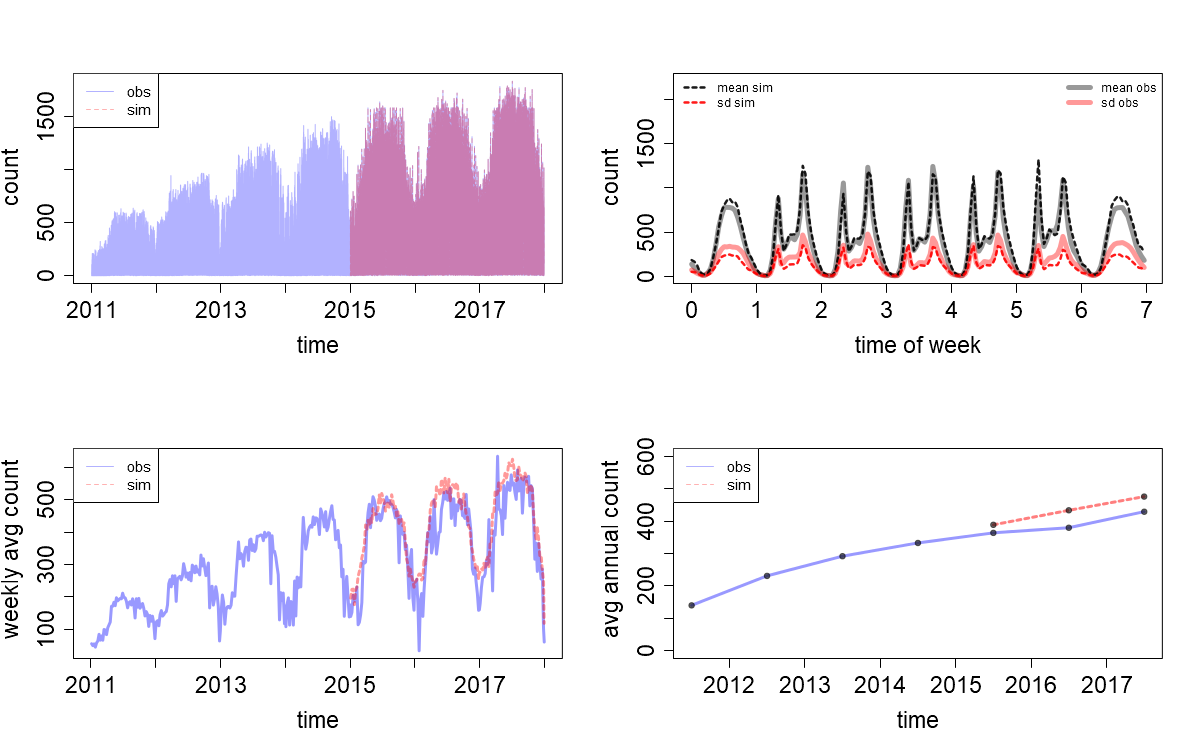
Figure 5: The simulation results from a Poisson conditional model with transformed lags and time-varying damping. The model is fitted on the data from 2011 to end of 2015 and the validation data is considered to be from 2016 to end of 2018. The Top Left Panel shows the result of one simulation added to the observed data. The Top Right Panel shows the average and standard deviation of counts for each hour of the week from the observed data (on the validation set) and the model simulations, showing a good agreement. The Bottom Left Panel shows the average hourly count for each week of observed data and compare that to the simulated values. The bottom Left Panel shows the average annual count from the observed data and compares it to the average annual count from simulated data.

7 Discussion

This paper developed models for count timeseries data which are able to capture complex trends over time in the mean and volatility of the process. We showed that by allowing complex dependence on various temporal scales and lags, even conditional Poisson models can achieve the volatility observed in the data.

In order to deal with the large number of parameters needed, we use the Grouped Structural Model Selection (GSMS) approach which works by grouping the covariates into various groups, each of which represent a structure in the model and then selecting the necessary covariates within each group in each step.

One challenge which is common in many timeseries applications is the possibility of explosive behavior in the simulations from the model. This problem is more likely, when there is significant non-linearity in the conditional mean and the $log$ is the link function. We tried some other link functions such as identity function, inverse and square root. However, in those cases, the models often did not converge – even after providing careful initial values for the parameters (e.g. by regressing the observed historical conditional probabilities on the covariates as discussed in R. Hosseini et al. (2012)). Moreover, while it is less likely to encounter explosive behavior with these link functions, we still observed explosive behavior in some cases. Based on these observations, we used the natural logarithm link function and to deal with the explosive behavior, we developed a method which works by damping the simulated response when it falls outside admissible intervals, which are defined using the observed data. To define the admissible intervals, we first defined some quantile-based measures of variability in the right and left sides/tails of the distribution. Using these variability measures, we developed a new definition for outliers which works better for asymmetric distributions. To improve flagging of outliers, we allowed the admissible interval to depend on other variables (in our data on the hour of week).

Appendix A Other simulations

In this section, we provide the results for various other models which do not use damping or lag transformation. In summary, the results indicate that damping and lag transformation (with $f(x)=\log(x+0.1)$ as the transformation) are beneficial in getting realistic simulations from the models.

A.1 Simulation with damping and no lag transformation

In this subsection, we apply the models with no lag transformation as opposed to using the log transform: $f(x)=\log(x+0.1)$.

As we discussed in the main text, the purpose of using transformed lag variables is to decrease the chance of explosive behavior of the simulated values. This method is also suggested in Fokianos (2012). We still continue to perform damping in this case, and the damping percentage can measure how much explosive behavior is observed as a result of no lag transformations. The results for the model fits are given in Table 5, which are comparable with the model fits with lag transformations. However, Table 6, shows that for the models which involve lags, a much higher percent of damping – more than 50% in some cases – is needed. This indicates that, while damping has kept the model simulations relatively realistic, the percentage of damping is very high – which questions the validity of the model in practice.

Family	Parameter Complexity	std AIC	std BIC	cor(obs, fitted)
Poisson	seas_only	57.80	57.80	0.84
Poisson	seas_growth	35.50	35.50	0.92
Poisson	seas_growth_longt	26.90	26.90	0.95
Poisson	seas_growth_lag	25.40	25.40	0.95
Poisson	seas_growth_longt_lag	24.60	24.70	0.95
NB	seas_only	11.20	11.20	0.83
NB	seas_growth	10.80	10.80	0.92
NB	seas_growth_longt	10.60	10.60	0.93
NB	seas_growth_lag	10.60	10.60	0.93
NB	seas_growth_longt_lag	10.50	10.50	0.93

Table 5: Model fit results models without lag transformation.

Family	Parameter Complexity	Percent Damping	RMSE	MAE	cor(obs, sim)
Poisson	seas_only	9.73	252.00	168.00	0.90
Poisson	seas_growth	12.20	177.00	110.00	0.91
Poisson	seas_growth_longt	51.10	373.00	255.00	0.85
Poisson	seas_growth_lag	25.20	256.00	160.00	0.84
Poisson	seas_growth_longt_lag	44.70	354.00	237.00	0.85
NB	seas_only	10.40	291.00	188.00	0.74
NB	seas_growth	16.60	241.00	155.00	0.81
NB	seas_growth_longt	50.10	374.00	255.00	0.82
NB	seas_growth_lag	30.90	306.00	201.00	0.79
NB	seas_growth_longt_lag	51.30	393.00	267.00	0.82

Table 6: Simulation results for damped models, without lag transformation

A.2 Simulation with lag transformation and no damping

In this subsection, we perform a simulation with lag transformation (as it is the case in the main text) but without damping. The simulation results are given in Table 7. We observe that the RMSE and MAE in this case are larger than the corresponding RMSE and MAE in Table 4 which used damping.

Family	Parameter Complexity	Percent Damping	RMSE	MAE	cor(obs, sim)
Poisson	seas_only	0.00	252.00	167.00	0.90
Poisson	seas_growth	0.00	178.00	110.00	0.91
Poisson	seas_growth_longt	0.00	180.00	111.00	0.90
Poisson	seas_growth_lag	0.00	198.00	121.00	0.88
Poisson	seas_growth_longt_lag	0.00	190.00	117.00	0.88
NB	seas_only	0.00	292.00	188.00	0.74
NB	seas_growth	0.00	283.00	173.00	0.78
NB	seas_growth_longt	0.00	260.00	158.00	0.80
NB	seas_growth_lag	0.00	252.00	155.00	0.80
NB	seas_growth_longt_lag	0.00	248.00	152.00	0.80

Table 7: Simulation results for undamped models with lag transformation.

References

- Akaike (1974) Akaike, H. (1974) A new look at the statistical model identification. IEEE Transactions on Automatic Control, AC-19:716–723.
- Berk and MacDonald (2008) Berk R. and MacDonald J. (2008) Overdispersion and Poisson regression. Journal of Quantitative Criminology. 24(3):269–284. doi:10.1007/s10940–008–9048–4.
- Chauvenet (1891) Chauvenet, W. (1891) A Manual of Spherical and Practical Astronomy, V. II. 1863. Reprint of 1891. 5th ed. Dover, N.Y.: 1960. 474–566.
- Efron (1986) Efron, B. (1986) Double exponential families and their use in generalized linear regression. Journal of the American Statistical Association, 81:709–721.
- Heinen (2003) Heinen A. (2003) Modelling time series count data: an autoregressive conditional poisson model. Center for Operations Research and Econometrics (CORE), Discussion Paper No. 2003–63, University of Louvain, Belgium
- Fanaee et al. (2013) Fanaee-T, Hadi, and Gama, Joao (2013) Event labeling combining ensemble detectors and background knowledge Progress in Artificial Intelligence, pp. 1–15, Springer Berlin Heidelberg.
- Fokianos (2012) Fokianos, K. (2012) Count Time Series Models Handbook of Statistics, Volume 30, Chapter 12, pp. 315–348 Time Series Analysis: Methods and Applications Edited by Rao, T. S., Rao, S. S. and Rao C.R.
- Hastie et al. (2009) Hastie, T., Tibshirani, R. and Friedman, J. H. (2009) The Elements of Statistical Learning, Second Edition. Springer
- Hosseini et al. (2011a) Hosseini, R., Le, N. and Zidek, J. (2011a) A Characterization of Categorical Markov Chains. Journal of Statistical Theory and Practice, 5(2):261–284
- Hosseini et al. (2011b) Hosseini, R., Le, N. and Zidek, J. (2011b) Selecting a binary Markov model for a precipitation process. Environmental and Ecological Statistics, 18(4):795–820
- R. Hosseini et al. (2012) Hosseini, R., Le, N. and Zidek, J. (2012) Time-Varying Markov Models for Binary Temperature Series in Agrorisk Management. Journal of Agricultural Biological and Ecological Statistics, 17(2):283–305
- Hosseini et al. (2015a) Hosseini, R., Takemura, A. and Hosseini, A. (2015a) Non-linear time-varying stochastic models for agroclimate risk assessment. Environmental and Ecological Statistics, 22(2):227–246.
- Hosseini et al. (2015b) Hosseini, R., Newlands, N. K., Dean, C. B. and Takemura, A. (2015b) Statistical modeling of soil moisture, integrating satellite remote-sensing (SAR) and ground-based data. Remote Sensing, 7(3):2752–2780
- Hosseini et al. (2017) Hosseini, A., Hosseini, R., Zare-Mehrjerdi, Y. and Abooie, M. H. (2017) Capturing the time-dependence in the precipitation process for weather risk assessment. Stochastic Environmental Research and Risk Assessment, 31(3):609–627
- Kedem et al. (2002) Kedem, B. and Fokianos, K. (2002) Regression Models for Time Series Analysis, Wiley Series in Probability and Statistics
- Nastic et al. (2012) Nastic, A. S., Ristic M. M. and Bakouch, H. S. (2012) A combined geometric INAR(p) model based on negative binomial thinning Mathematical and Computer Modelling, 55:1665–1672
- Schwartz (1978) Schwartz, G. (1978) Estimating the dimension of a model. Annals of Statistics, 6:461–464.
- Thall and Veil (1990) Thall, P. F. and Vail, S. C. (1990) Some covariance models for longitudinal count data with overdispersion Biometrics, 46(3):657–671
- Tong (1990) Tong, H. (1990) Non-linear time series, a dynamical systems approach. Oxford University Press
- Tukey (1977) Tukey, J. W. (1977). Exploratory Data Analysis. Addison-Wesley. ISBN 978-0-201-07616-5. OCLC 3058187
- Upton (1996) Upton, G., Cook, I. (1996) Understanding Statistics. Oxford University Press. p. 55. ISBN 0-19-914391-9.
- Ver Hoef and Boveng (2007) Ver Hoef, J. M. and Boveng, P. L. (2007) Quasi-Poisson vs. Negative Binomial Regression: How should we model overdispersed count data. Ecology, 88(11): 2766–2772. doi:10.1890/07–0043.1.
- Weiß (2009) Weiß, C. H. (2009) Modelling time series of counts with over-dispersion Statistical Methods and Applications, 18(4):507–519
- Wong (1986) Wong, W. (1986) Theory of Partial Likelihood. Annals of Statistics, 14(1):88–123
- Yang et al. (2016) Yang, Z., Hu, J., Shu, Y., Cheng, P., Chen, J. and Moscibroda, T. (2016) Mobility Modeling and Prediction in Bike-Sharing Systems ACM International Conference on Mobile Systems, Applications, and Services (MobiSys), June 25–30, 2016, Singapore, Singapore
- Yule (1911) Yule, G. U. (1911) An Introduction to the Theory of Statistics. Charles Griffin and Company. pp. 147–148
- Zheng et al (2006) Zheng, T., Salganik, M. J. and Gelman, A. (2006) How Many People Do You Know in Prison? Journal of the American Statistical Association, 101(474):409–423, doi:10.1198/016214505000001168