The asymptotic spectrum of flipped multilevel Toeplitz matrices and of certain preconditionings

Abstract

In this work, we perform a spectral analysis of flipped multilevel Toeplitz sequences, i.e., we study the asymptotic spectral behaviour of $\{Y_{\boldsymbol{n}}T_{\boldsymbol{n}}(f)\}_{\boldsymbol{n}}$, where $T_{\boldsymbol{n}}(f)$ is a real, square multilevel Toeplitz matrix generated by a function $f\in L^{1}([-\pi,\pi]^{d})$ and $Y_{\boldsymbol{n}}$ is the exchange matrix, which has $1$s on the main anti-diagonal. In line with what we have shown for unilevel flipped Toeplitz matrix sequences, the asymptotic spectrum is determined by a $2\times 2$ matrix-valued function whose eigenvalues are $\pm|f|$. Furthermore, we characterize the eigenvalue distribution of certain preconditioned flipped multilevel Toeplitz sequences with an analysis that covers both multilevel Toeplitz and circulant preconditioners. Finally, all our findings are illustrated by several numerical experiments.

65F08, 65F10, 15B05

1 Introduction

In [5, 11] it was independently shown that when $T_{n}(f)\in\mathbb{R}^{n\times n}$ is a Toeplitz matrix generated by a function $f\in L^{1}([-\pi,\pi])$ then the eigenvalues of $Y_{n}T_{n}(f)$ are distributed like $\pm|f|$, where

$$Y_{n}=\begin{bmatrix}&&1\\ &\iddots&\\ 1&&\end{bmatrix}.$$

In this note, we show that this result also holds true when the Toeplitz matrix $T_{n}(f)$ is replaced by a multilevel Toeplitz matrix $T_{\boldsymbol{n}}(f)\in\mathbb{R}^{d_{\boldsymbol{n}}\times d_{\boldsymbol{n}}}$ and $Y_{n}$ is replaced by

$$Y_{\boldsymbol{n}}=Y_{n_{1}}\otimes\cdots\otimes Y_{n_{d}},$$

where $f\in L^{1}([-\pi,\pi]^{d})$, $\boldsymbol{n}=(n_{1},\ldots,n_{d})$ and $d_{\boldsymbol{n}}=n_{1}\dotsm n_{d}$. More specifically, we prove that the eigenvalues of $Y_{\boldsymbol{n}}T_{\boldsymbol{n}}(f)$ behave like the eigenvalues of the matrix-valued symbol

(1) $$g=\begin{bmatrix}&f\\ f^{\ast}&\end{bmatrix},$$

where $f^{\ast}$ is the conjugate of $f$, i.e., the eigenvalues of the flipped multilevel Toeplitz matrix $Y_{\boldsymbol{n}}T_{\boldsymbol{n}}(f)$ are distributed like $\pm|f|$.

Describing the spectra of these flipped matrices is important for solving linear systems with $T_{\boldsymbol{n}}(f)$ as coefficient matrix. Since a (multilevel) Toeplitz matrix can be symmetrized by the flip matrix, the resulting linear system may be solved by MINRES or preconditioned MINRES, with its short term recurrences and descriptive convergence theory based on eigenvalues [14, 15]. Hence, knowledge of the spectrum of $Y_{\boldsymbol{n}}T_{\boldsymbol{n}}(f)$ is critical for accurately estimating the MINRES convergence rate, and developing and analysing effective preconditioners. With this in mind, we characterize the eigenvalue distribution of certain preconditioned flipped multilevel Toeplitz sequences with an analysis that covers both multilevel Toeplitz and circulant preconditioners.

The paper is organized as follows. Section 2 provides background material and preliminary results. The key results are then presented in Section 3, and illustrated by numerical experiments in Section 4. Our conclusions can be found in Section 5.

2 Preliminaries

In this section we formalize the definition of multilevel (block) Toeplitz sequences associated with a Lebesgue integrable (matrix-valued) function. Next, we define the spectral distribution, in the sense of the eigenvalues and of the singular values, of a generic matrix sequence. To deal with the spectral distribution of preconditioned flipped multilevel Toeplitz matrices, we introduce a class of matrix sequences (the multilevel block GLT class) that contains multilevel block Toeplitz sequences.

2.1 Notation

To describe multilevel matrices we require multi-indices, $\boldsymbol{k}=(k_{1},\dotsc,k_{d})$, that we denote by bold letters. Whenever we use the expression ${{\boldsymbol{k}}\to\infty}$, we mean that every component of the vector ${\boldsymbol{k}}$ tends to infinity, that is, $\min_{\ell=1,\dots,d}k_{\ell}\to\infty$.

The complex conjugates of a scalar $\alpha$, and scalar-valued function $f(\boldsymbol{\theta})$, where $\boldsymbol{\theta}=(\theta_{1},\theta_{2},\dotsc,\theta_{d})$, $d\geq 1$, are denoted by $\alpha^{\ast}$ and $f^{\ast}(\boldsymbol{\theta})$, respectively. Similarly, the conjugate transpose of a vector $x$ is $x^{\ast}$, and the conjugate transpose of a matrix $X$ is $X^{\ast}$. Additionally, by $|f(\boldsymbol{\theta})|$ we mean $|f(\boldsymbol{\theta})|=\left(f(\boldsymbol{\theta})f^{*}(\boldsymbol{\theta})\right)^{1/2}$. The $n\times n$ identity matrix is $I_{n}$.

Throughout, by $d$-level $s\times s$-block matrix sequences we mean sequences of matrices of the form $\{A_{\boldsymbol{n}}\}_{n}$, where the index $n$ varies in an infinite subset of $\mathbb{N}$ and $\boldsymbol{n}=\boldsymbol{n}(n)$ is a $d$-index with positive components that depends on $n$ and satisfies $\boldsymbol{n}\rightarrow\infty$ as $n\rightarrow\infty$. The size of $A_{\boldsymbol{n}}$ is $s\cdot d_{\boldsymbol{n}}=sn_{1}\cdots n_{d}$. We will equivalently use the notation “$\{A_{\boldsymbol{n}}\}_{\boldsymbol{n}}$” to mean “$\{A_{\boldsymbol{n}}\}_{n}$”.

2.2 Multilevel block Toeplitz matrices and their spectral properties

In Definition 2.1 we introduce the notion of multilevel block Toeplitz matrix sequences generated by $f$.

Definition 2.1.

Let $f:[-\pi,\pi]^{d}\rightarrow\mathbb{C}^{s\times s}$, $d,s\geq 1$, where $f=[f_{ij}]_{i,j=1}^{s}$ is such that $f_{ij}\in L^{1}([-\pi,\pi]^{d})$. Let the Fourier coefficients of $f$ be given by

$$t_{\boldsymbol{k}}:=\frac{1}{(2\pi)^{d}}\int_{[-\pi,\pi]^{d}}f(\boldsymbol{\theta})\,\mathrm{e}^{-\boldsymbol{\mathrm{i}}\langle\boldsymbol{k},\boldsymbol{\theta}\rangle}\,\mathrm{d}\boldsymbol{\theta}\in\mathbb{C}^{s\times s},\quad\boldsymbol{k}=(k_{1},\dotsc,k_{d})\in\mathbb{Z}^{d},$$

where the integrals are computed componentwise and $\langle\boldsymbol{k},\boldsymbol{\theta}\rangle=\sum_{\ell=1}^{d}k_{\ell}\theta_{\ell}$. The $\boldsymbol{n}$-th $d$-level $s\times s$-block Toeplitz matrix associated with $f$ is the matrix of order $s\cdot d_{\boldsymbol{n}}$, $d_{\boldsymbol{n}}=n_{1}\dotsm n_{d}$, given by

$$T_{\boldsymbol{n}}(f)=\sum_{|k_{1}|<n_{1}}\dotsb\sum_{|k_{d}|<n_{d}}J_{n_{1}}^{(k_{1})}\otimes\dotsb\otimes J_{n_{d}}^{(k_{d})}\otimes t_{\boldsymbol{k}},$$

where $J_{n}^{(\ell)}$ is the matrix of dimension $n$ whose ($i,j$) entry is 1 if $i-j=\ell$ and is zero otherwise. The set $\{T_{\boldsymbol{n}}(f)\}_{\boldsymbol{n}}$ is called the family of multilevel block Toeplitz matrices generated by $f$. The function $f$ is referred to as the generating function of $\{T_{\boldsymbol{n}}(f)\}_{\boldsymbol{n}}$.

We now discuss the spectra of multilevel block Toeplitz matrices. To clarify the sense in which the function $f$ provides information on the spectrum for these problems, we need to introduce the following definition.

Definition 2.2.

Let $f:G\to\mathbb{R}^{s\times s}$ be a measurable function, defined on a measurable set $G\subset\mathbb{R}^{d}$ with $d\geq 1$, $0<m_{\ell}(G)<\infty$. Let $\mathcal{C}_{0}(\mathbb{K})$ be the set of continuous functions with compact support over $\mathbb{K}\in\{\mathbb{C},\mathbb{R}_{0}^{+}\}$ and let $\{A_{\boldsymbol{n}}\}_{\boldsymbol{n}}$, ${\boldsymbol{n}}\in\mathbb{N}^{v}$ $v\geq 1$, be a sequence of matrices with eigenvalues $\lambda_{j}(A_{\boldsymbol{n}})$, $j=1,\ldots,d_{\boldsymbol{n}}$ and singular values $\sigma_{j}(A_{\boldsymbol{n}})$, $j=1,\ldots,d_{\boldsymbol{n}}$, where $d_{\boldsymbol{n}}={\rm dim}(A_{\boldsymbol{n}})$ is a monotonic function with respect to each variable $n_{i}$, $i=1,\ldots,v$.

• We say that $\{A_{\boldsymbol{n}}\}_{\boldsymbol{n}}$ is distributed as the pair $(f,G)$ in the sense of the eigenvalues, and we write $\{A_{\boldsymbol{n}}\}_{\boldsymbol{n}}\sim_{\lambda}(f,G),$ if the following limit relation holds for all $F\in\mathcal{C}_{0}(\mathbb{C})$:

  (2) $$\lim_{{\boldsymbol{n}}\to\infty}\frac{1}{d_{\boldsymbol{n}}}\sum_{j=1}^{d_{\boldsymbol{n}}}F(\lambda_{j}(A_{\boldsymbol{n}}))=\frac{1}{m_{\ell}(G)}\int_{G}\frac{{\rm tr}(F(f(\boldsymbol{\theta})))}{s}d\boldsymbol{\theta}.$$

  In this case, we say that f is the symbol of the matrix sequence $\{A_{\boldsymbol{n}}\}_{\boldsymbol{n}}$.

• We say that $\{A_{\boldsymbol{n}}\}_{\boldsymbol{n}}$ is distributed as the pair $(f,G)$ in the sense of the singular values, and we write $\{A_{\boldsymbol{n}}\}_{\boldsymbol{n}}\sim_{\sigma}(f,G),$ if the following limit relation holds for all $F\in\mathcal{C}_{0}(\mathbb{R}_{0}^{+})$:

  (3) $$\lim_{{\boldsymbol{n}}\to\infty}\frac{1}{d_{\boldsymbol{n}}}\sum_{j=1}^{d_{\boldsymbol{n}}}F(\sigma_{j}(A_{\boldsymbol{n}}))=\frac{1}{m_{\ell}(G)}\int_{G}\frac{{\rm tr}(F(|f(\boldsymbol{\theta})|))}{s}d\boldsymbol{\theta}.$$

Recall that in this setting the expression ${{\boldsymbol{n}}\to\infty}$ means that every component of the vector ${\boldsymbol{n}}$ tends to infinity, that is, $\min_{i=1,\dots,v}n_{i}\to\infty$.

Remark 2.3.

If $f$ is smooth enough, an informal interpretation of the limit relation Eq. 2 (resp. Eq. 3) is that when $\boldsymbol{n}$ is sufficiently large, $d_{\boldsymbol{n}}/s$ eigenvalues (resp. singular values) of $A_{\boldsymbol{n}}$ can be approximated by a sampling of $\lambda_{1}(f)$ (resp. $\sigma_{1}(f)$) on a uniform equispaced grid of the domain $G$, and so on until the last $d_{\boldsymbol{n}}/s$ eigenvalues (resp. singular values), which can be approximated by an equispaced sampling of $\lambda_{s}(f)$ (resp. $\sigma_{s}(f)$) in the domain.

The above definitions are applicable to multilevel Toeplitz matrix sequences, as the following theorem (due to Szegő, Tilli, Zamarashkin, Tyrtyshnikov, …) shows.

Theorem 2.4 (see [10, 17, 18]).

Let $\{T_{\boldsymbol{n}}(f)\}_{\boldsymbol{n}}$ be a multilevel Toeplitz sequence generated by $f\in L^{1}([-\pi,\pi]^{d})$. Then, $\left\{T_{\boldsymbol{n}}(f)\right\}_{\boldsymbol{n}}\sim_{\sigma}(f,[-\pi,\pi]^{d}).$ Moreover, if $f$ is real-valued, then $\left\{T_{\boldsymbol{n}}(f)\right\}_{\boldsymbol{n}}\sim_{\lambda}(f,[-\pi,\pi]^{d}).$

In the case that $f$ is a Hermitian matrix-valued function, the previous theorem can be extended as follows:

Theorem 2.5 (see [17]).

Let $f:[-\pi,\pi]^{d}\rightarrow\mathbb{C}^{s\times s}$, $d>1$, with $f=[f_{ij}]_{i,j=1}^{s}$ such that $f_{ij}\in L^{1}([-\pi,\pi]^{d})$, be a Hermitian matrix-valued function. Then, $\{T_{\boldsymbol{n}}(f)\}_{\boldsymbol{n}}\sim_{\lambda}(f,[-\pi,\pi]^{d}).$

The following theorem is a useful tool for computing the spectral distribution of a sequence of Hermitian matrices. For its proof, see [12, Theorem 4.3].

Theorem 2.6.

Let $f:G\subset\mathbb{R}^{d}\rightarrow\mathbb{C}^{s\times s}$, let $\{X_{\boldsymbol{n}}\}_{\boldsymbol{n}}$ be a sequence of matrices with $X_{\boldsymbol{n}}$ Hermitian of size $d_{\boldsymbol{n}}$, and let $\{P_{\boldsymbol{n}}\}_{\boldsymbol{n}}$ be a sequence such that $P_{\boldsymbol{n}}\in\mathbb{C}^{d_{\boldsymbol{n}}\times\delta_{\boldsymbol{n}}}$, $P_{\boldsymbol{n}}^{*}P_{\boldsymbol{n}}=I_{\delta_{\boldsymbol{n}}}$, $\delta_{\boldsymbol{n}}\leq d_{\boldsymbol{n}}$ and $\delta_{\boldsymbol{n}}/d_{\boldsymbol{n}}\to 1$ as $\boldsymbol{n}\to\infty$. Then $\{X_{\boldsymbol{n}}\}_{\boldsymbol{n}}\sim_{\lambda}(f,G)$ if and only if $\{P_{\boldsymbol{n}}^{*}X_{\boldsymbol{n}}P_{\boldsymbol{n}}\}_{\boldsymbol{n}}\sim_{\lambda}(f,G)$.

2.3 Multilevel block generalized locally Toeplitz class

In the sequel, we introduce the $*$-algebra of multilevel block generalized locally Toeplitz (GLT) matrix sequences [6, 7]. The formal definition of this class is rather technical and involves somewhat cumbersome notation: therefore we just give and briefly discuss a few properties of the multilevel block GLT class, which are sufficient for studying the spectral features of preconditioned flipped multilevel Toeplitz matrices.

Throughout, we use the notation

$$\{A_{\boldsymbol{n}}\}_{\boldsymbol{n}}\sim_{\rm GLT}{\kappa(\boldsymbol{x},\boldsymbol{\theta})},\quad\ \ \kappa:[0,1]^{d}\times[-\pi,\pi]^{d}\rightarrow\mathbb{C}^{s\times s}$$

to indicate that the sequence $\{A_{\boldsymbol{n}}\}_{\boldsymbol{n}}$ is a $d$-level $s\times s$-block GLT sequence with GLT symbol $\kappa(\boldsymbol{x},\boldsymbol{\theta})$.

Here we list five of the main features of multilevel block GLT sequences.

• Let $\{A_{\boldsymbol{n}}\}_{\boldsymbol{n}}\sim_{\rm GLT}\kappa$ with $\kappa:G\rightarrow\mathbb{C}^{s\times s}$, $G=[0,1]^{d}\times[-\pi,\pi]^{d}$. Then $\{A_{\boldsymbol{n}}\}_{\boldsymbol{n}}\sim_{\sigma}(\kappa,G)$. If the matrices $A_{\boldsymbol{n}}$ are Hermitian, then it also holds that $\{A_{\boldsymbol{n}}\}_{\boldsymbol{n}}\sim_{\lambda}(\kappa,G)$.

• The set of block GLT sequences forms a $*$-algebra, i.e., it is closed under linear combinations, products, inversion and conjugation. In formulae, let $\{A_{\boldsymbol{n}}\}_{\boldsymbol{n}}\sim_{\rm GLT}\kappa_{1}$ and $\{B_{\boldsymbol{n}}\}_{\boldsymbol{n}}\sim_{\rm GLT}\kappa_{2}$, then

  • $\{\alpha A_{\boldsymbol{n}}+\beta B_{\boldsymbol{n}}\}_{\boldsymbol{n}}\sim_{\rm GLT}\alpha\kappa_{1}+\beta\kappa_{2},\quad\alpha,\beta\in\mathbb{C};$

  • $\{A_{\boldsymbol{n}}B_{\boldsymbol{n}}\}_{\boldsymbol{n}}\sim_{\rm GLT}\kappa_{1}\kappa_{2};$

  • $\{A^{-1}_{\boldsymbol{n}}\}_{\boldsymbol{n}}\sim_{\rm GLT}\kappa_{1}^{-1}$ provided that $\kappa_{1}$ is invertible a.e.;

  • $\{A_{\boldsymbol{n}}^{*}\}_{\boldsymbol{n}}\sim_{\rm GLT}{\kappa^{*}_{1}}.$

• Any sequence of multilevel block Toeplitz matrices $\{T_{\boldsymbol{n}}(f)\}_{\boldsymbol{n}}$ generated by a function $f:[-\pi,\pi]^{d}\rightarrow\mathbb{C}^{s\times s}$, with $f=[f_{ij}]_{i,j=1}^{s}$ such that $f_{ij}\in L^{1}([-\pi,\pi]^{d})$, is a $d$-level $s\times s$-block GLT sequence with symbol $\kappa(\boldsymbol{x},\boldsymbol{\theta})=f(\boldsymbol{\theta})$.

• Let $\{A_{\boldsymbol{n}}\}_{\boldsymbol{n}}\sim_{\sigma}0$. We say that $\{A_{\boldsymbol{n}}\}_{\boldsymbol{n}}$ is a zero-distributed matrix sequence. Note that for any $s>1$ $\{A_{\boldsymbol{n}}\}_{\boldsymbol{n}}\sim_{\sigma}O_{s}$, with $O_{s}$ the $s\times s$ null matrix, is equivalent to $\{A_{\boldsymbol{n}}\}_{\boldsymbol{n}}\sim_{\sigma}0$. Every zero-distributed matrix sequence is a block GLT sequence with symbol $O_{s}$ and viceversa, i.e., $\{A_{\boldsymbol{n}}\}_{\boldsymbol{n}}\sim_{\sigma}0$ $\iff$ $\{A_{\boldsymbol{n}}\}_{\boldsymbol{n}}\sim_{\rm GLT}O_{s}$.

• Let $\{A_{\boldsymbol{n}}\}_{\boldsymbol{n}}$ be a $d$-level matrix sequence and let $\{B_{\boldsymbol{n},m}\}_{\boldsymbol{n}}$ be a sequence of matrix sequences that satisfies the following condition: for each $m$ there exists $n_{m}$, such that for $m>n_{m}$

  $$A_{\boldsymbol{n}}=B_{\boldsymbol{n},m}+R_{\boldsymbol{n},m}+E_{\boldsymbol{n},m}$$

  with

  $${\rm rank}(R_{\boldsymbol{n},m})<c(m)d_{\boldsymbol{n}},\quad\|E_{\boldsymbol{n},m}\|\leq\omega(m),\quad\lim_{m\rightarrow\infty}c(m),\omega(m)=0.$$

  We say that $\{B_{\boldsymbol{n},m}\}$ is an “a.c.s.” (approximating class of sequences) for $\{A_{\boldsymbol{n}}\}_{\boldsymbol{n}}$, and we write $\{B_{\boldsymbol{n},m}\}_{\boldsymbol{n}}\xrightarrow{a.c.s.}\{A_{\boldsymbol{n}}\}_{\boldsymbol{n}}$. Moreover, $\{A_{\boldsymbol{n}}\}_{\boldsymbol{n}}\sim_{\rm GLT}\kappa$ if and only if there exist GLT sequences $\{B_{\boldsymbol{n},m}\}_{\boldsymbol{n}}\sim_{\rm GLT}\kappa_{m}$ and $\kappa_{m}\rightarrow\kappa$ in measure.

The following proposition provides an a.c.s. for a sequence of multilevel block Toeplitz matrices (see [9]).

Proposition 2.7.

Let $\{f_{m}\}_{m}$ be a sequence of d-variate trigonometric matrix-valued polynomials with $f_{m}:[-\pi,\pi]^{d}\rightarrow\mathbb{C}^{s\times s}$, $f_{m}=[(f_{m})_{ij}]_{i,j=1}^{s}$ such that $(f_{m})_{ij}\in L^{1}([-\pi,\pi]^{d})$. If $(f_{m})_{ij}\rightarrow(f)_{ij}$ in $L^{1}([-\pi,\pi]^{d})$, then the sequence $\{T_{\boldsymbol{n}}(f_{m})\}_{\boldsymbol{n}}$ satisfies

$$\{T_{\boldsymbol{n}}(f_{m})\}_{\boldsymbol{n}}{\xrightarrow{a.c.s.}}\{T_{\boldsymbol{n}}(f)\}_{\boldsymbol{n}}.$$

We also give an additional characterization of zero-distributed matrix sequences that will prove useful:.

Theorem 2.8 (see [9, Theorem 2.2]).

Let $\{A_{\boldsymbol{n}}\}_{\boldsymbol{n}}$ be a sequence of matrices with $A_{\boldsymbol{n}}$ of dimension $d_{\boldsymbol{n}}$. Then $\{A_{\boldsymbol{n}}\}_{\boldsymbol{n}}\sim_{\sigma}0$ if and only if, for every $\boldsymbol{n}$,

$$A_{\boldsymbol{n}}=R_{\boldsymbol{n}}+E_{\boldsymbol{n}},\qquad\lim_{\boldsymbol{n}\to\infty}\frac{{\rm rank}(R_{\boldsymbol{n}})}{d_{\boldsymbol{n}}}=0,\qquad\lim_{\boldsymbol{n}\to\infty}\|E_{\boldsymbol{n}}\|=0.$$

We next recall a result on the spectral distribution of Hankel sequences associated with $f:[-\pi,\pi]^{d}\rightarrow\mathbb{C}^{s\times s}$, where $f=[f_{ij}]_{i,j=1}^{s}$ is such that $f_{ij}\in L^{1}([-\pi,\pi]^{d})$.

Theorem 2.9 (see [4]).

Let $\{H_{\boldsymbol{n}}(f)\}_{\boldsymbol{n}}$ be the $\boldsymbol{n}$-th $s\times s$-block multilevel Hankel matrix associated with $f:[-\pi,\pi]^{d}\rightarrow\mathbb{C}^{s\times s}$, where $f=[f_{ij}]_{i,j=1}^{s}$ is such that $f_{ij}\in L^{1}([-\pi,\pi]^{d})$. If $H_{\boldsymbol{n}}(f)$ is the $sd_{\boldsymbol{n}}\times sd_{\boldsymbol{n}}$ matrix

$$H_{\boldsymbol{n}}(f)=\left[t_{\boldsymbol{i}+\boldsymbol{j}-\boldsymbol{2}}\right]_{\boldsymbol{i},\boldsymbol{j}=\boldsymbol{1}}^{\boldsymbol{n}},$$

with $t_{\boldsymbol{k}}\in\mathbb{C}^{s\times s}$ the Fourier coefficients of $f$, then $\{H_{\boldsymbol{n}}(f)\}_{\boldsymbol{n}}\sim_{\sigma}0$.

Remark 2.10.

Note that one can equivalently take $H_{\boldsymbol{n}}(f)=\left[t_{\boldsymbol{2}-\boldsymbol{i}-\boldsymbol{j}}\right]_{\boldsymbol{i},\boldsymbol{j}=\boldsymbol{1}}^{\boldsymbol{n}}$ in Theorem 2.9.

Together, Theorem 2.9 and GLT4 tell us that $\{H_{\boldsymbol{n}}(f)\}_{\boldsymbol{n}}$ is an $s\times s$-block GLT sequence with symbol $O_{s}$.

We end this subsection with a theorem that is very useful in the context of preconditioning involving GLT matrix sequences. It is obtained as a straightforward extension of Theorem 1 in [8] to the multilevel block GLT case, provided the symbol of the preconditioning sequence is a multiple of the identity.

Theorem 2.11.

Let $\{A_{\boldsymbol{n}}\}_{\boldsymbol{n}}$ be a sequence of Hermitian matrices such that $\{A_{\boldsymbol{n}}\}_{\boldsymbol{n}}\sim_{\rm GLT}\kappa$, with $\kappa:G\rightarrow\mathbb{C}^{s\times s}$, $G=[0,1]^{d}\times[-\pi,\pi]^{d}$, and let $\{\mathcal{P}_{\boldsymbol{n}}\}_{\boldsymbol{n}}$ be a sequence of Hermitian positive definite matrices such that $\{\mathcal{P}_{\boldsymbol{n}}\}_{\boldsymbol{n}}\sim_{\rm GLT}h\cdot I_{s}$, with $h:G\rightarrow\mathbb{C}$, such that $h\neq 0$ a.e. Then,

$$\{\mathcal{P}_{\boldsymbol{n}}^{-1}A_{\boldsymbol{n}}\}_{\boldsymbol{n}}\sim_{\sigma,\lambda}(h^{-1}\kappa,G).$$

3 Main result

In this section we prove the main result, namely that $\{Y_{\boldsymbol{n}}T_{\boldsymbol{n}}(f)\}_{\boldsymbol{n}}{\sim_{\lambda}}(g,[-\pi,\pi]^{d})$, where $g$ is given in Eq. 1 and the dimension of $T_{\boldsymbol{n}}(f)$ is given by the multi-index $\boldsymbol{n}=(n_{1},\dotsc,n_{d})$.

We first introduce the following matrices:

• $\Pi_{\boldsymbol{n}}=\Pi_{n_{1}}\otimes\Pi_{n_{2}}\otimes\cdots\otimes\Pi_{n_{d}}$ with $\Pi_{n_{k}}$, $n_{k}$ even, such that its $j$-th column $\pi_{j}$, $j=1,\dotsc,n_{k}$, is

  $$\pi_{j}=\begin{cases}e_{2j-1},&j=1,\dotsc,n_{k}/2,\\ e_{2(j-n_{k}/2)},&j=n_{k}/2+1,\dotsc,n_{k},\end{cases}$$

  where $e_{j}$, $j=1,\dotsc,n_{k}$, is the $j$-th column of the identity matrix of dimension $n_{k}$;

• $Y_{\boldsymbol{n}}=Y_{n_{1}}\otimes Y_{n_{2}}\otimes\cdots\otimes Y_{n_{d}}$ with $Y_{n_{k}}$ defined as

  $$Y_{n_{k}}=\begin{bmatrix}&&1\\ &\iddots&\\ 1&&\end{bmatrix}_{n_{k}\times n_{k}};$$

• $U_{\boldsymbol{n}}=U_{n_{1}}\otimes U_{n_{2}}\otimes\cdots\otimes U_{n_{d}}$ with $U_{n_{k}}$ such that

  $$U_{n_{k}}=\begin{bmatrix}Y_{\lceil n_{k}/2\rceil}&\\ &I_{\lfloor n_{k}/2\rfloor}\end{bmatrix}.$$

We now state an important preliminary result.

Proposition 3.1.

Assume that $\boldsymbol{n}=(n_{1},\ldots,n_{d})$ with $n_{k}=2m_{k}$, $m_{k}\in\mathbb{N}$. Then, for any $f\in L^{1}([-\pi,\pi]^{d}])$,

$$\{\Pi_{\boldsymbol{n}}U_{\boldsymbol{n}}Y_{\boldsymbol{n}}T_{\boldsymbol{n}}(f)U_{\boldsymbol{n}}\Pi_{\boldsymbol{n}}^{T}\}_{\boldsymbol{n}}\sim_{\rm GLT}(g,[-\pi,\pi]^{d})\text{\,\,\, with \,\,\,}g:=\begin{bmatrix}0&f\\ f^{\ast}&0\end{bmatrix}.$$

Proof 3.2.

Let us first assume that $f(\boldsymbol{\theta})=f_{\boldsymbol{q}}(\boldsymbol{\theta})=\sum_{\boldsymbol{j}=-\boldsymbol{q}}^{\boldsymbol{q}}t_{\boldsymbol{j}}{\rm e}^{\boldsymbol{\mathrm{i}}\langle\boldsymbol{j},\boldsymbol{\theta}\rangle}$. Then,

$$\Pi_{\boldsymbol{n}}U_{\boldsymbol{n}}Y_{\boldsymbol{n}}T_{\boldsymbol{n}}(f_{\boldsymbol{q}})U_{\boldsymbol{n}}\Pi_{\boldsymbol{n}}^{T}$$

$$=\Pi_{\boldsymbol{n}}U_{\boldsymbol{n}}Y_{\boldsymbol{n}}\left(\sum_{\boldsymbol{j}=-\boldsymbol{q}}^{\boldsymbol{q}}t_{\boldsymbol{j}}T_{\boldsymbol{n}}\left(\prod_{k=1}^{d}{\rm e}^{\boldsymbol{\mathrm{i}}j_{k}\theta_{k}}\right)\right)U_{\boldsymbol{n}}\Pi_{\boldsymbol{n}}^{T}$$

$$=\Pi_{\boldsymbol{n}}U_{\boldsymbol{n}}Y_{\boldsymbol{n}}\left(\sum_{\boldsymbol{j}=-\boldsymbol{q}}^{\boldsymbol{q}}t_{\boldsymbol{j}}T_{n_{1}}({\rm e}^{\boldsymbol{\mathrm{i}}j_{1}\theta_{1}})\otimes\cdots\otimes T_{n_{d}}({\rm e}^{\boldsymbol{\mathrm{i}}j_{d}\theta_{d}})\right)U_{\boldsymbol{n}}\Pi_{\boldsymbol{n}}^{T}$$

$$=\sum_{\boldsymbol{j}=-\boldsymbol{q}}^{\boldsymbol{q}}t_{\boldsymbol{j}}\,\,\Pi_{n_{1}}U_{n_{1}}Y_{n_{1}}T_{n_{1}}({\rm e}^{\boldsymbol{\mathrm{i}}j_{1}\theta_{1}})U_{n_{1}}\Pi_{n_{1}}^{T}\otimes\cdots\otimes\Pi_{n_{d}}U_{n_{d}}Y_{n_{d}}T_{n_{d}}({\rm e}^{\boldsymbol{\mathrm{i}}j_{d}\theta_{d}})U_{n_{d}}\Pi^{T}_{n_{d}}.$$

Now, by using Lemmas 3.1 and 3.2 in [11] applied to $f(\theta_{k})={\rm e}^{\boldsymbol{\mathrm{i}}j_{k}\theta_{k}}$ we find that

$$\Pi_{n_{k}}U_{n_{k}}Y_{n_{k}}T_{n_{k}}({\rm e}^{\boldsymbol{\mathrm{i}}j_{k}\theta_{k}})U_{n_{k}}\Pi_{n_{k}}^{T} =T_{n_{k}}\left(\begin{bmatrix}0&{\rm e}^{\boldsymbol{\mathrm{i}}j_{k}\theta_{k}}\\ {\rm e}^{-\boldsymbol{\mathrm{i}}j_{k}\theta_{k}}&0\end{bmatrix}\right)+E_{n_{k}}+R_{n_{k}}$$

with

$$\lim_{n_{k}\rightarrow\infty}\frac{{\rm rank}(R_{n_{k}})}{n_{k}}=0,\,\,\lim_{n_{k}\rightarrow\infty}\|E_{n_{k}}\|=0.$$

Therefore,

$$\Pi_{\boldsymbol{n}}U_{\boldsymbol{n}}Y_{\boldsymbol{n}}T_{\boldsymbol{n}}(f_{\boldsymbol{q}})U_{\boldsymbol{n}}\Pi_{\boldsymbol{n}}^{T}$$

$$=\sum_{\boldsymbol{j}=-\boldsymbol{q}}^{\boldsymbol{q}}t_{\boldsymbol{j}}\,\,\left(T_{n_{1}}\left(\begin{bmatrix}0&{\rm e}^{\boldsymbol{\mathrm{i}}j_{1}\theta_{1}}\\ {\rm e}^{-\boldsymbol{\mathrm{i}}j_{1}\theta_{1}}&0\end{bmatrix}\right)+E_{n_{1}}+R_{n_{1}}\right)\otimes\cdots$$

$$\cdots\otimes\left(T_{n_{d}}\left(\begin{bmatrix}0&{\rm e}^{\boldsymbol{\mathrm{i}}j_{d}\theta_{d}}\\ {\rm e}^{-\boldsymbol{\mathrm{i}}j_{d}\theta_{d}}&0\end{bmatrix}\right)+E_{n_{d}}+R_{n_{d}}\right)$$

$$=\sum_{\boldsymbol{j}=-\boldsymbol{q}}^{\boldsymbol{q}}t_{\boldsymbol{j}}\,\,T_{n_{1}}\left(\begin{bmatrix}0&{\rm e}^{\boldsymbol{\mathrm{i}}j_{1}\theta_{1}}\\ {\rm e}^{-\boldsymbol{\mathrm{i}}j_{1}\theta_{1}}&0\end{bmatrix}\right)\otimes\cdots\otimes T_{n_{d}}\left(\begin{bmatrix}0&{\rm e}^{\boldsymbol{\mathrm{i}}j_{d}\theta_{d}}\\ {\rm e}^{-\boldsymbol{\mathrm{i}}j_{d}\theta_{d}}&0\end{bmatrix}\right)+R_{\boldsymbol{n}}+E_{\boldsymbol{n}}$$

(4) $$=T_{\boldsymbol{n}}\left(\begin{bmatrix}0&f_{\boldsymbol{q}}\\ f_{\boldsymbol{q}}^{\ast}&0\end{bmatrix}\right)+R_{\boldsymbol{n}}+E_{\boldsymbol{n}}$$

with

$$\lim_{\boldsymbol{n}\rightarrow\infty}\frac{{\rm rank}(R_{\boldsymbol{n}})}{d_{\boldsymbol{n}}}=0,\,\,\lim_{\boldsymbol{n}\rightarrow\infty}\|E_{\boldsymbol{n}}\|=0,$$

or equivalently

$${\left\{T_{\boldsymbol{n}}\left(\begin{bmatrix}0&f_{\boldsymbol{q}}\\ f_{\boldsymbol{q}}^{\ast}&0\end{bmatrix}\right)\right\}_{\boldsymbol{n}}}\xrightarrow{a.c.s.}\{\Pi_{\boldsymbol{n}}U_{\boldsymbol{n}}Y_{\boldsymbol{n}}T_{\boldsymbol{n}}(f_{\boldsymbol{q}})U_{\boldsymbol{n}}\Pi_{\boldsymbol{n}}^{T}\}_{\boldsymbol{n}}.$$

Thanks to GLT2–4 and Theorem 2.8 the thesis is proven for $f=f_{\boldsymbol{q}}$ a trigonometric polynomial.

Let us now switch to a generic $f\in L^{1}([-\pi,\pi]^{d})$. It is well known that the set of $d$-variate polynomials is dense in $L^{1}([-\pi,\pi]^{d})$. Therefore, there exists a sequence of polynomials $f_{m}:[-\pi,\pi]^{d}\rightarrow\mathbb{C}$ such that $f_{m}\rightarrow f\in L^{1}([-\pi,\pi]^{d})$. By Proposition 2.7 $\{T_{\boldsymbol{n}}(f_{m})\}_{n}{\xrightarrow{a.c.s.}}\{T_{\boldsymbol{n}}(f)\}_{\boldsymbol{n}}$ i.e., for every $m$ there exists $n_{m}$ such that, for $n>n_{m}$,

$$T_{\boldsymbol{n}}(f)=T_{\boldsymbol{n}}(f_{m})+R_{\boldsymbol{n},m}+E_{\boldsymbol{n},m}$$

with

$${\rm rank}(R_{\boldsymbol{n},m})<c(m)d_{\boldsymbol{n}},\quad\|E_{\boldsymbol{n},m}\|\leq\omega(m),\quad\lim_{m\rightarrow\infty}c(m),\omega(m)=0.$$

Now, by 3.2 we have

$$\Pi_{\boldsymbol{n}}U_{\boldsymbol{n}}Y_{\boldsymbol{n}}T_{\boldsymbol{n}}(f)U_{\boldsymbol{n}}\Pi_{\boldsymbol{n}}^{T}$$

$$=\Pi_{\boldsymbol{n}}U_{\boldsymbol{n}}Y_{\boldsymbol{n}}T_{\boldsymbol{n}}(f_{m})U_{\boldsymbol{n}}\Pi_{\boldsymbol{n}}^{T}+\Pi_{\boldsymbol{n}}U_{\boldsymbol{n}}Y_{\boldsymbol{n}}R_{\boldsymbol{n},m}U_{\boldsymbol{n}}\Pi_{\boldsymbol{n}}^{T}+\Pi_{\boldsymbol{n}}U_{\boldsymbol{n}}Y_{\boldsymbol{n}}E_{\boldsymbol{n},m}U_{\boldsymbol{n}}\Pi_{\boldsymbol{n}}^{T}$$

$$=T_{\boldsymbol{n}}\left(\begin{bmatrix}0&f_{m}\\ f_{m}^{\ast}&0\end{bmatrix}\right)+\underbrace{R_{\boldsymbol{n}}+\Pi_{\boldsymbol{n}}U_{\boldsymbol{n}}Y_{\boldsymbol{n}}R_{\boldsymbol{n},m}U_{\boldsymbol{n}}\Pi_{\boldsymbol{n}}^{T}}_{\tilde{R}}+\underbrace{E_{\boldsymbol{n}}+\Pi_{\boldsymbol{n}}U_{\boldsymbol{n}}Y_{\boldsymbol{n}}E_{\boldsymbol{n},m}U_{\boldsymbol{n}}\Pi_{\boldsymbol{n}}^{T}}_{\tilde{E}}$$

with

$${\rm rank}({\tilde{R}})<\tilde{c}(m)d_{\boldsymbol{n}},\quad\|{\tilde{E}}\|\leq\tilde{\omega}(m),\quad\lim_{m\rightarrow\infty}\tilde{c}(m),\tilde{\omega}(m)=0.$$

Then,

$$\left\{T_{\boldsymbol{n}}\left(\begin{bmatrix}0&f_{m}\\ f_{m}^{\ast}&0\end{bmatrix}\right)\right\}_{n}{\xrightarrow{a.c.s.}}\{\Pi_{\boldsymbol{n}}U_{\boldsymbol{n}}Y_{\boldsymbol{n}}T_{\boldsymbol{n}}(f)U_{\boldsymbol{n}}\Pi_{\boldsymbol{n}}^{T}\}_{\boldsymbol{n}}.$$

This together with $\left\{\begin{bmatrix}0&f_{m}\\ f_{m}^{\ast}&0\end{bmatrix}\right\}_{m}\rightarrow\begin{bmatrix}0&f\\ f^{\ast}&0\end{bmatrix}$ with $f\in L^{1}([-\pi,\pi]^{d})$, and GLT3 and GLT5, concludes the proof.

Remark 3.3.

Assume that $n_{k}=2m_{k}+1$ with $m_{k}\in\mathbb{N}$. Then, $U_{n_{k}}Y_{n_{k}}T_{n_{k}}({\rm e}^{\boldsymbol{\mathrm{i}}j_{k}\theta_{k}})U_{n_{k}}$ can be embedded into the $(2m_{k}+2)\times(2m_{k}+2)$ matrix

$$A_{n_{k}+1}$$

$$=\begin{bmatrix}H_{m_{k}+1}({\rm e}^{\boldsymbol{\mathrm{i}}j_{k}\theta_{k}})&T_{m_{k}+1}({\rm e}^{\boldsymbol{\mathrm{i}}j_{k}\theta_{k}})\\ T_{m_{k}+1}({\rm e}^{-\boldsymbol{\mathrm{i}}j_{k}\theta_{k}})&H_{m_{k}+1}({\rm e}^{-\boldsymbol{\mathrm{i}}j_{k}\theta_{k}})\end{bmatrix}$$

$$=\Pi_{n_{k}+1}^{T}T_{2m_{k}+2}\left(\begin{bmatrix}0&{\rm e}^{\boldsymbol{\mathrm{i}}j_{k}\theta_{k}}\\ {\rm e}^{-\boldsymbol{\mathrm{i}}j_{k}\theta_{k}}&0\end{bmatrix}\right)\Pi_{n_{k}+1}$$

$$\hskip 14.22636pt+\Pi_{n_{k}+1}^{T}H_{2m_{k}+2}\left(\begin{bmatrix}{\rm e}^{\boldsymbol{\mathrm{i}}j_{k}\theta_{k}}&0\\ 0&{\rm e}^{-\boldsymbol{\mathrm{i}}j_{k}\theta_{k}}\end{bmatrix}\right)\Pi_{n_{k}+1}$$

$$=\Pi_{n_{k}+1}^{T}T_{2m_{k}+2}\left(\begin{bmatrix}0&{\rm e}^{\boldsymbol{\mathrm{i}}j_{k}\theta_{k}}\\ {\rm e}^{-\boldsymbol{\mathrm{i}}j_{k}\theta_{k}}&0\end{bmatrix}\right)\Pi_{n_{k}+1}$$

$$\hskip 14.22636pt+R_{2m_{k}+2}+E_{2m_{k}+2}$$

where $H(\cdot)$ is the (block) Hankel matrix generated by the function specified by the brackets and the last equality follows from Theorem 2.9 combined with Theorem 2.8. Specifically,

$$U_{n_{k}}Y_{n_{k}}T_{n_{k}}({\rm e}^{\boldsymbol{\mathrm{i}}j_{k}\theta_{k}})U_{n_{k}}=PA_{n_{k}+1}P^{T},$$

with

$$P=\begin{bmatrix}I_{m+1}&{\bf 0}&O_{(m+1)\times m}\\ O_{m\times(m+1)}&{\bf 0}&I_{m}\end{bmatrix}\text{ and }{\bf 0}=(0,\ldots,0)^{T}.$$

On this basis, using the same line of proof as for Proposition 3.1 shows that the matrix $U_{\boldsymbol{n}}Y_{\boldsymbol{n}}T_{\boldsymbol{n}}(f)U_{\boldsymbol{n}}$ is a principal submatrix of a matrix that, after a proper permutation, gives rise to a GLT sequence whose symbol is $g$.

Remark 3.4.

Assume that $\boldsymbol{n}=(n_{1},\ldots,n_{d})$ with $n_{k}=2m_{k}$, $m_{k}\in\mathbb{N}$. Then, the line of proof used for Proposition 3.1 shows that

$$\{\Pi_{\boldsymbol{n}}T_{\boldsymbol{n}}(f)\Pi_{\boldsymbol{n}}^{T}\}\sim_{\rm GLT}\begin{bmatrix}f&0\\ 0&f\end{bmatrix}$$

and

(5) $$\{\Pi_{\boldsymbol{n}}U_{\boldsymbol{n}}T_{\boldsymbol{n}}(f)U_{\boldsymbol{n}}\Pi_{\boldsymbol{n}}^{T}\}\sim_{\rm GLT}\begin{bmatrix}f^{\ast}&0\\ 0&f\end{bmatrix}.$$

Remark 3.5.

Assume that $\boldsymbol{n}=(n_{1},\ldots,n_{d})$ with $n_{k}=2m_{k}$, $m_{k}\in\mathbb{N}$. Then,

$$\Pi_{\boldsymbol{n}}U_{\boldsymbol{n}}Y_{\boldsymbol{n}}U_{\boldsymbol{n}}\Pi_{\boldsymbol{n}}^{T} =\Pi_{n_{1}}U_{n_{1}}Y_{n_{1}}U_{n_{1}}\Pi_{n_{1}}^{T}\otimes\cdots\otimes\Pi_{n_{d}}U_{n_{d}}Y_{n_{d}}U_{n_{d}}\Pi^{T}_{n_{d}}$$

$$=T_{n_{1}}\left(\begin{bmatrix}0&1\\ 1&0\end{bmatrix}\right)\otimes\cdots\otimes T_{n_{d}}\left(\begin{bmatrix}0&1\\ 1&0\end{bmatrix}\right)$$

$$=T_{\boldsymbol{n}}\left(\begin{bmatrix}0&1\\ 1&0\end{bmatrix}\right).$$

Hence, using Eq. 5 we arrive at the same result as in Proposition 3.1, i.e.,

$$\{\Pi_{\boldsymbol{n}}U_{\boldsymbol{n}}Y_{\boldsymbol{n}}T_{\boldsymbol{n}}(f)U_{\boldsymbol{n}}\Pi_{\boldsymbol{n}}^{T}\}$$

$$=\{\Pi_{\boldsymbol{n}}U_{\boldsymbol{n}}Y_{\boldsymbol{n}}U_{\boldsymbol{n}}\Pi_{\boldsymbol{n}}^{T}\Pi_{\boldsymbol{n}}U_{\boldsymbol{n}}T_{\boldsymbol{n}}(f)U_{\boldsymbol{n}}\Pi_{\boldsymbol{n}}^{T}\}\sim_{\rm GLT}\begin{bmatrix}0&1\\ 1&0\end{bmatrix}\begin{bmatrix}f^{\ast}&0\\ 0&f\end{bmatrix}=g.$$

We can now state the main theorem of this section, which describes the spectral distribution of $\{Y_{\boldsymbol{n}}T_{\boldsymbol{n}}(f)\}_{\boldsymbol{n}}$.

Theorem 3.6.

Let $\{T_{\boldsymbol{n}}(f)\}_{\boldsymbol{n}}$, $T_{\boldsymbol{n}}(f)\in\mathbb{R}^{d_{\boldsymbol{n}}\times d_{\boldsymbol{n}}}$ be the multilevel Toeplitz sequence associated with $f\in L^{1}([-\pi,\pi]^{d})$,  where $\boldsymbol{n}=(n_{1},\ldots,n_{d})$ and $d_{\boldsymbol{n}}=n_{1}\dotsm n_{d}$. Let $\{Y_{\boldsymbol{n}}T_{\boldsymbol{n}}(f)\}_{\boldsymbol{n}}$ be the corresponding sequence of flipped Toeplitz matrices. Then,

(6) $$\{Y_{\boldsymbol{n}}T_{\boldsymbol{n}}(f)\}_{\boldsymbol{n}}\sim_{\lambda}(g,[-\pi,\pi]^{d}),\text{\,\,\, with \,\,\,}g=\begin{bmatrix}0&f\\ f^{\ast}&0\end{bmatrix}.$$

Proof 3.7.

In the case that $n_{k}=2m_{k}$, $m_{k}\in\mathbb{N}$ for each $k$, we see from Proposition 3.1 that $\{\Pi_{\boldsymbol{n}}U_{\boldsymbol{n}}Y_{\boldsymbol{n}}T_{\boldsymbol{n}}(f)U_{\boldsymbol{n}}\Pi_{\boldsymbol{n}}^{T}\}\sim_{\rm GLT}g$. Hence, recalling that $\Pi_{\boldsymbol{n}}U_{\boldsymbol{n}}Y_{\boldsymbol{n}}T_{\boldsymbol{n}}(f)U_{\boldsymbol{n}}\Pi_{\boldsymbol{n}}^{T}$ is real symmetric, by GLT1, $\{Y_{\boldsymbol{n}}T_{\boldsymbol{n}}(f)\}\sim_{\lambda}g$. In all other cases, by recalling Remark 3.3 and using Theorem 2.6 we find that the thesis follows as well.

We end this section by providing the spectral distribution of a preconditioned sequence of flipped multilevel Toeplitz matrices.

Theorem 3.8.

Let $\{T_{\boldsymbol{n}}(f)\}_{\boldsymbol{n}}$, $T_{\boldsymbol{n}}(f)\in\mathbb{R}^{d_{\boldsymbol{n}}\times d_{\boldsymbol{n}}}$ with $n_{k}=2m_{k}$, $m_{k}\in\mathbb{N}$ be the multilevel Toeplitz sequence associated with $f\in L^{1}([-\pi,\pi]^{d})$, let $\{Y_{\boldsymbol{n}}T_{\boldsymbol{n}}(f)\}_{\boldsymbol{n}}$ be the corresponding sequence of flipped multilevel Toeplitz matrices, and let $\{\mathcal{P}_{\boldsymbol{n}}\}_{\boldsymbol{n}}$ be a sequence of Hermitian positive definite matrices such that $\{\mathcal{P}_{\boldsymbol{n}}\}_{\boldsymbol{n}}\sim_{\rm GLT}h$, and $\{\Pi_{\boldsymbol{n}}U_{\boldsymbol{n}}\mathcal{P}_{\boldsymbol{n}}U_{\boldsymbol{n}}\Pi_{\boldsymbol{n}}^{T}\}_{\boldsymbol{n}}\sim_{\rm GLT}h\cdot I_{2}$ with $h:[-\pi,\pi]^{d}\rightarrow\mathbb{C}$ and $h\neq 0$ a.e. Then,

(7) $$\{\mathcal{P}_{\boldsymbol{n}}^{-1}Y_{\boldsymbol{n}}T_{\boldsymbol{n}}(f)\}_{\boldsymbol{n}}\sim_{\lambda}(h^{-1}g,[-\pi,\pi]^{d}).$$

Proof 3.9.

The thesis follows from the combination of Theorem 2.11 and Proposition 3.1 by noticing that

$$(\Pi_{\boldsymbol{n}}U_{\boldsymbol{n}}\mathcal{P}_{\boldsymbol{n}}U_{\boldsymbol{n}}\Pi_{\boldsymbol{n}}^{T})^{-1}U_{\boldsymbol{n}}\Pi_{\boldsymbol{n}}Y_{\boldsymbol{n}}T_{\boldsymbol{n}}(f)U_{\boldsymbol{n}}\Pi_{\boldsymbol{n}}^{T}=\Pi_{\boldsymbol{n}}U_{\boldsymbol{n}}\mathcal{P}_{\boldsymbol{n}}^{-1}Y_{\boldsymbol{n}}T_{\boldsymbol{n}}(f)U_{\boldsymbol{n}}\Pi_{\boldsymbol{n}}^{T}$$

and by recalling that $Y_{\boldsymbol{n}}T_{\boldsymbol{n}}(f)$ is real symmetric and that $\Pi_{\boldsymbol{n}}U_{\boldsymbol{n}}$ is orthogonal.

Note that, thanks to Remark 3.4, the hypotheses of Theorem 3.8 are satisfied in the case where $\mathcal{P}_{\boldsymbol{n}}=T_{\boldsymbol{n}}(h)$, with $h\geq 0$ and $h\neq 0$ a.e. Moreover, it easy to see that if we take the following circulant preconditioner

$$\mathcal{P}_{\boldsymbol{n}}=C_{\boldsymbol{n}}=|C_{n_{d}}|\otimes\cdots\otimes I_{n_{1}}+\cdots+I_{n_{d}}\otimes\cdots\otimes|C_{n_{1}}|$$

with $|C_{n_{\ell}}|=(C_{n_{\ell}}^{T}C_{n_{\ell}})^{\frac{1}{2}}$ where $C_{n_{\ell}}$ is the optimal preconditioner for $T_{n_{\ell}}=T_{n_{\ell}}(f_{\ell})$, the condition $\{\Pi_{\boldsymbol{n}}U_{\boldsymbol{n}}C_{\boldsymbol{n}}U_{\boldsymbol{n}}\Pi_{\boldsymbol{n}}^{T}\}_{\boldsymbol{n}}\sim_{\rm GLT}h\cdot I_{2}$ holds as well. This is because both $\{|C_{n_{\ell}}|\}_{n_{\ell}}$ and $\{T(|f_{\ell}|)\}_{n_{\ell}}$ are GLTs with symbol $|f_{\ell}|$ and then $|C_{n_{\ell}}|=T(|f_{\ell}|)+R_{n_{\ell}}+E_{n_{\ell}}$ which allows us to apply the same reasoning as in Remark 3.4 to prove the desired relation.

4 Numerical results

In this section we illustrate the theoretical results from Section 3, that is, we check the validity of Theorems 3.6 and 3.8. We start by defining the following equispaced grid on $[0,\pi]^{d}$:

$$\Gamma=\left\{(\theta^{(k_{1})}_{1},\ldots,\theta^{(k_{d})}_{d}):=\left(\frac{\pi k_{1}}{\left\lfloor\frac{n_{1}}{2}\right\rfloor-1},\frac{\pi k_{2}}{n_{2}-1},\ldots,\frac{\pi k_{d}}{n_{d}-1}\right),\begin{array}[]{rl}k_{1}=&0,\ldots,\left\lfloor\frac{n_{1}}{2}\right\rfloor-1,\\ k_{j}=&0,\dots,n_{j}-1,\\ j=&2,\ldots,d\end{array}\right\}.$$

Then, we denote by $\Lambda_{1}$ and $\Lambda_{2}$ the set of all evaluations of $\lambda_{1}(g)$, $\lambda_{2}(g)$ (resp. $\lambda_{1}(h^{-1}g)$, $\lambda_{2}(h^{-1}g)$) on $\Gamma$, and by $\Lambda$ the union $\Lambda_{1}\cup\Lambda_{2}$ ordered in an ascending way. In the following examples we numerically check relation Eq. 6 (resp. Eq. 7) by comparing the eigenvalues of $Y_{\boldsymbol{n}}T_{\boldsymbol{n}}(f)$ (resp. $\mathcal{P}_{n}^{-1}Y_{\boldsymbol{n}}T_{\boldsymbol{n}}(f)$) with the values collected in $\Lambda$. Note that it suffices to consider only $[0,\pi]^{d}$ in place of $[-\pi,\pi]^{d}$ because the eigenvalue functions of the considered symbols are even.

In the two-dimensional Examples 4.1 and 4.2 we also compare the eigenvalues of $Y_{\boldsymbol{n}}T_{\boldsymbol{n}}(f)$ directly with the spectrum of $g$ over the whole domain $[-\pi,\pi]^{2}$. Precisely, we define the following grid on $[-\pi,\pi]^{2}$

$$\Delta=\left\{(\theta^{(\ell)}_{1},\theta^{(\kappa)}_{2}):=\left(-\pi+\frac{2\pi\ell}{n_{1}-1},-\pi+\frac{2\pi\kappa}{n_{2}-1}\right),\begin{array}[]{rl}\ell=&0,\dots,n_{1}-1,\\ \kappa=&0,\dots,n_{2}-1\end{array}\right\}$$

and again we denote by $\Lambda_{1}$ and $\Lambda_{2}$ the sets of all evaluations of $\lambda_{1}(g)$, $\lambda_{2}(g)$ on $\Delta$, and by $\Lambda$ the union $\Lambda_{1}\cup\Lambda_{2}$ ordered in an ascending way. Therefore, we employ the following matching algorithm: for a fixed eigenvalue $\lambda$ of $Y_{\boldsymbol{n}}T_{\boldsymbol{n}}(f)$

1. we find $\tilde{\eta}\in\Lambda$ such that $\|\lambda-\tilde{\eta}\|=\min_{\eta\in\Lambda}\|\lambda-\eta\|$, and

2. we associate $\lambda$ to the couple in $\Delta$ that corresponds to $\tilde{\eta}$.

Example 4.1.

The first example we consider is the $2$-level banded Toeplitz matrix generated by $f(\theta_{1},\theta_{2})=4+\mathrm{e}^{\boldsymbol{\mathrm{i}}\theta_{1}}+\mathrm{e}^{\boldsymbol{\mathrm{i}}\theta_{2}}$. We see from Fig. 1 that the uniform sampling of eigenvalue functions of $g$ collected in $\Lambda$ accurately describes the eigenvalues of $Y_{\boldsymbol{n}}T_{\boldsymbol{n}}(f)$, even for very small matrices. Moreover, as shown in Fig. 2 (obtained using the aforementioned matching algorithm), the eigenvalues of $Y_{\boldsymbol{n}}T_{\boldsymbol{n}}(f)$ accurately mimic the shape of the eigenvalue functions of $g$ when $n_{1}=20,n_{2}=40$.

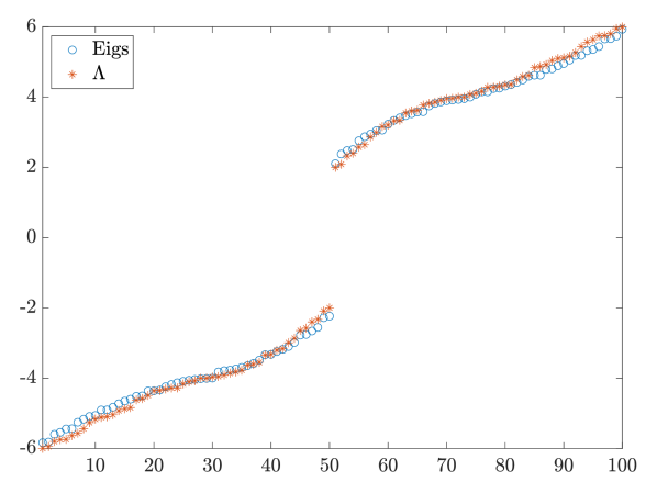
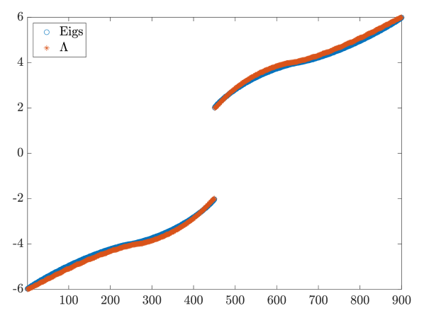
Figure 1: Comparison of the eigenvalues of $Y_{\boldsymbol{n}}T_{\boldsymbol{n}}(f)$ ( $\circ$) with $\Lambda$ collecting the uniform samples of the eigenvalue functions of $g$ for Example 4.1 ($\ast$) when $n_{1}=n_{2}=10$ (left) and $n_{1}=n_{2}=30$ (right).

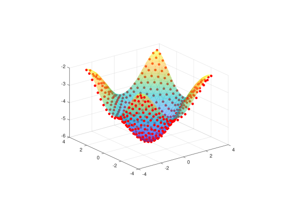
(a) $\lambda_{1}(g)=-|f|$

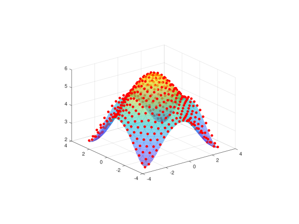
(b) $\lambda_{2}(g)=|f|$

Figure 2: Eigenvalues of $Y_{\boldsymbol{n}}T_{\boldsymbol{n}}(f)$ (red dots) and the spectrum of $g$ (colored surfaces) for Example 4.1 when $n_{1}=20$ and $n_{2}=40$.

Example 4.2.

In this example we consider the dense $2$-level Toeplitz matrix obtained by discretizing a certain time-dependent initial-boundary fractional diffusion problem by means of a second-order finite difference approximation that combines the Crank-Nicolson scheme and the so-called weighted and shifted Grünwald formula (see [16]). Precisely, we start from

$$\begin{cases}\frac{\partial u(x,y,t)}{\partial t}=\frac{\partial^{\alpha}u(x,y,t)}{\partial_{+}x^{\alpha}}+\frac{\partial^{\beta}u(x,y,t)}{\partial_{+}y^{\beta}}+v(x,y,t),\qquad\qquad&(x,y,t)\in\Omega\times(0,1],\\ u(x,y,t)=0,&(x,y,t)\in{\mathbb{R}^{2}\backslash\Omega}\times[0,1],\\ u(x,y,0)=u_{0}(x,y),&(x,y)\in\bar{\Omega},\end{cases}$$

where $\Omega=(0,1)\times(0,1)$, $\alpha,\beta\in(1,2)$, and $\frac{\partial^{\alpha}u(x,y,t)}{\partial_{+}x^{\alpha}}$, $\frac{\partial^{\alpha}u(x,y,t)}{\partial_{+}y^{\beta}}$ are fractional derivatives defined in Riemann-Liouville form (see again [2]). Then, for fixed $n_{1},n_{2},M\in\mathbb{N}$, we take the following equispaced partition of $\Omega\times[0,1]$

$$x_{i}=ih_{x}, \quad h_{x}=\frac{1}{n_{1}+1}, \quad i=0,1,\dots,n_{1},$$

$$y_{j}=jh_{y}, \quad h_{y}=\frac{1}{n_{2}+1}, \quad j=0,1,\dots,n_{2},$$

$$t^{(m)}=m\Delta t, \;\Delta t=\frac{1}{M},\quad \quad m=0,1,\dots,M,$$

and we arrive at a linear system whose coefficient matrix is the $2$-level Toeplitz matrix

$$\mathbf{\mathcal{M}}^{(\alpha,\beta)}_{\boldsymbol{n}} =\frac{2h_{x}^{\alpha}}{\Delta t}I_{n_{1}n_{2}}+I_{n_{2}}\otimes T_{n_{1}}(f_{\alpha})+\frac{h_{x}^{\alpha}}{h_{x}^{\beta}}T_{n_{2}}(f_{\beta})\otimes I_{n_{1}},$$

with $\boldsymbol{n}=(n_{1},n_{2})$,

$$f_{\gamma}(\theta)=-\sum_{k=-1}^{\infty}w_{k+1}^{(\beta)}{\rm e}^{\mathbf{i}k\theta}=-\bigg{[}\frac{2-\gamma(1-{\rm e}^{-\mathbf{i}\theta})}{2}\bigg{]}\left(1+{\rm e}^{\mathbf{i}(\theta+\pi)}\right)^{\gamma},$$

$\gamma\in\{\alpha,\beta\}$, $\theta\in\{\theta_{1},\theta_{2}\}$, and $w_{k}^{(\beta)}$ defined as in [16]. Both $T_{n_{1}}(f_{\alpha})$ and $T_{n_{2}}(f_{\beta})$ are lower Hessenberg, and so $\mathbf{\mathcal{M}}^{(\alpha,\beta)}_{\boldsymbol{n}}$ is non-symmetric.

It has been shown in [13] that, whenever $\frac{h_{x}^{\alpha}}{h_{x}^{\beta}}=O(1)$ and $\frac{2h_{x}^{\alpha}}{\Delta t}=o(1)$, it holds that

$$\{\mathbf{\mathcal{M}}^{(\alpha,\beta)}_{\boldsymbol{n}}\}_{\boldsymbol{n}}\sim_{\lambda}f_{\alpha,\beta}:=f_{\alpha}(\theta_{1})+\frac{h_{x}^{\alpha}}{h_{x}^{\beta}}f_{\beta}(\theta_{2}),$$

i.e., $\mathbf{\mathcal{M}}^{(\alpha,\beta)}_{\boldsymbol{n}}=T_{\boldsymbol{n}}(f_{\alpha,\beta})$.

In the following tests we fix $\alpha=1.8$ and $\beta=1.6$. Fig. 3(a) shows that when $M=n_{1}=30$ and $n_{2}=35$ the eigenvalues of the flipped Toeplitz matrix $Y_{\boldsymbol{n}}T_{\boldsymbol{n}}(f)$ are well described by the sampling of the eigenvalue functions of $g$ given in $\Lambda$. Similar results can be inferred from Fig. 4 when comparing the eigenvalues of $Y_{\boldsymbol{n}}T_{\boldsymbol{n}}(f)$ directly when the spectrum of $g$ with $n_{1}=20$, $n_{2}=40$.

For this example we also show how the results in Section 3 can be used to describe the convergence rate of preconditioned MINRES, which depends heavily on the spectral properties of the coefficient matrix (see, e.g., [3, Chapters 2 & 4]). With this aim we focus on the solution of the following linear system

$$T_{\boldsymbol{n}}(f_{\alpha,\beta})u_{\boldsymbol{n}}=b_{\boldsymbol{n}},$$

with $b_{\boldsymbol{n}}=2h_{x}^{\alpha}\boldsymbol{1}$, and we define the following preconditioners for $Y_{\boldsymbol{n}}T_{\boldsymbol{n}}(f_{\alpha,\beta})$:

• $\mathcal{P}_{\boldsymbol{n}}=T_{\boldsymbol{n}}(f_{R})$, with $f_{R}=\frac{f_{\alpha,\beta}+f^{\ast}_{\alpha,\beta}}{2}$. Of course, in this case the symbol of the preconditioning matrix sequence is $h=f_{R}$;

• $\mathcal{P}_{\boldsymbol{n}}=P^{2,2}_{\boldsymbol{n}}$, obtained from $\mathbf{\mathcal{M}}^{(\alpha,\beta)}_{\boldsymbol{n}}$ replacing $T_{n_{1}}(f_{\alpha})$, $T_{n_{2}}(f_{\beta})$, with $T_{n_{1}}(2-2\cos\theta_{1})$, $T_{n_{2}}(2-2\cos\theta_{2})$, respectively (see [13] for more details). In this case, the symbol of the preconditioning matrix sequence is $h=2-2\cos\theta_{1}+\frac{h_{x}^{\alpha}}{h_{x}^{\beta}}(2-2\cos\theta_{2})$;

• $\mathcal{P}_{\boldsymbol{n}}=P^{2,\beta}_{\boldsymbol{n}}$, obtained from $\mathbf{\mathcal{M}}^{(\alpha,\beta)}_{\boldsymbol{n}}$ replacing $T_{n_{1}}(f_{\alpha})$ with $T_{n_{1}}(2-2\cos(\theta_{1}))$, and $T_{n_{2}}(f_{\beta})$ with the real part of its tetra-diagonal band truncation $T_{n_{2}}(p_{\beta}(\theta_{2}))$, where

  $$p_{\beta}(\theta_{2})=-\sum_{k=-1}^{2}w_{k+1}^{(\beta)}{\rm e}^{\i k\theta_{2}}.$$

  In this case, the symbol of the preconditioning matrix sequence is $h=2-2\cos\theta_{1}+\frac{h_{x}^{\alpha}}{h_{x}^{\beta}}\frac{p_{\beta}(\theta_{2})+p^{\ast}_{\beta}(\theta_{2})}{2}$.

All of the aforementioned preconditioners are symmetric positive definite matrices that satisfy the conditions of Theorem 3.8 when $\boldsymbol{n}=(n_{1},n_{2})$ has even components. Fig. 3(b)–(d) show that the eigenvalues of $\mathcal{P}_{\boldsymbol{n}}^{-1}Y_{\boldsymbol{n}}T_{\boldsymbol{n}}(f)$ are well described by the sampling of the eigenvalue functions of $h^{-1}g$ contained in $\Lambda$ even though not all components of $\boldsymbol{n}$ are even, as required by Theorem 3.8 (here $n_{1}=30$ and $n_{2}=35$). Moreover, in all the given cases the eigenvalues of the preconditioned matrices lie close to $1$ and $-1$. This is particularly evident for $\mathcal{P}_{\boldsymbol{n}}=T_{\boldsymbol{n}}(f_{R})$. Note that, when $\mathcal{P}_{\boldsymbol{n}}=P_{\boldsymbol{n}}^{2,\beta}$, the eigenvalue functions of $h^{-1}g$ assume values around zero (while the eigenvalues of $\mathcal{P}_{\boldsymbol{n}}^{-1}Y_{\boldsymbol{n}}T_{\boldsymbol{n}}(f)$ do not); this is because $p_{\beta}(\theta_{2})$ does not have a zero at $\theta_{2}=0$ but $f_{\beta}(\theta_{2})$ does.

From Fig. 3(b)–(d) and since $\lambda_{1}(h^{-1}g),\lambda_{2}(h^{-1}g)$ are clustered at $\pm 1$, we expect that preconditioned MINRES applied to the flipped version of Example 4.2 with preconditioners $T_{\boldsymbol{n}}(f_{R})$, $P_{\boldsymbol{n}}^{2,2}$ or $P_{\boldsymbol{n}}^{2,\beta}$ will converge at a fast rate. In Table 1 the iterations of preconditioned MINRES are stopped when the residual norm is reduced by eight orders of magnitude, i.e, when $\|r_{k}\|_{2}/\|r_{0}\|_{2}<10^{-8}$. We see from these results that for all three preconditioners convergence is rapid, with $T_{\boldsymbol{n}}(f_{R})$ resulting in the lowest iteration counts. Neither $P_{\boldsymbol{n}}^{2,2}$ nor $P_{\boldsymbol{n}}^{2,\beta}$ is optimal and this is in line with the spectral analysis performed in [13, 2]. On the other hand, both are block banded with banded block matrices, and so are computationally affordable unlike the dense preconditioner $T_{\boldsymbol{n}}(f_{R})$.

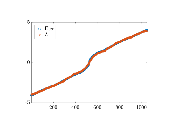
(a) Unpreconditioned

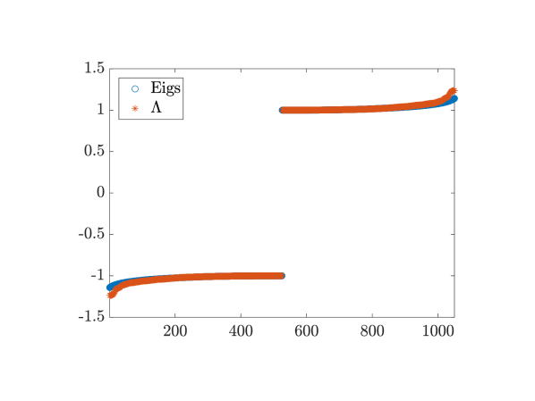
(b) $\mathcal{P}_{\boldsymbol{n}}=T_{\boldsymbol{n}}(f_{R})$

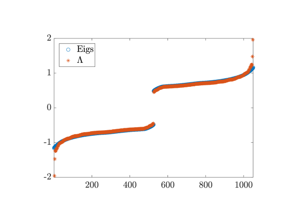
(c) $\mathcal{P}_{\boldsymbol{n}}=P^{2,2}_{\boldsymbol{n}}$

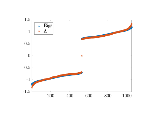
(d) $\mathcal{P}_{\boldsymbol{n}}=P^{2,\beta}_{\boldsymbol{n}}$

Figure 3: Comparison of the eigenvalues of $Y_{\boldsymbol{n}}T_{\boldsymbol{n}}(f_{\alpha,\beta})$ or $\mathcal{P}_{\boldsymbol{n}}^{-1}Y_{\boldsymbol{n}}T_{\boldsymbol{n}}(f_{\alpha,\beta})$ ( $\circ$) with $\Lambda$ collecting the uniform samples of the eigenvalue functions of $g$ or $h^{-1}g$ for Example 4.2 ($\ast$) when $M=n_{1}=30$, $n_{2}=35$.

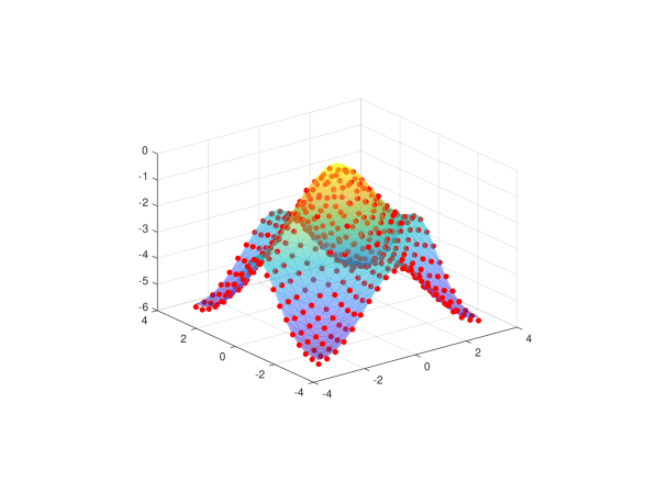
(a) $\lambda_{1}(g)=-|f|$

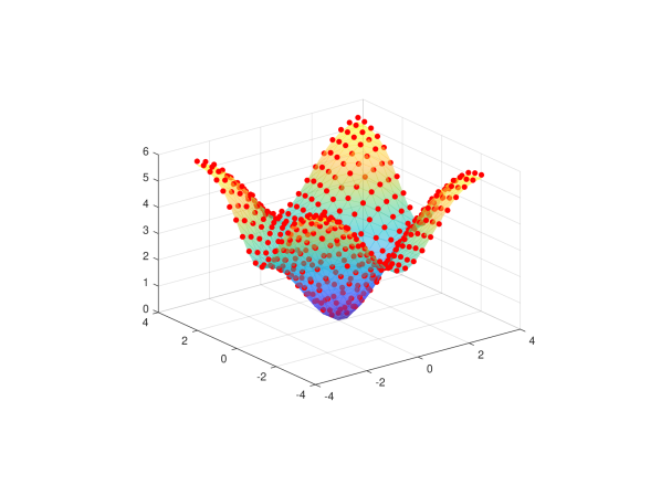
(b) $\lambda_{2}(g)=|f|$

Figure 4: Eigenvalues of $Y_{\boldsymbol{n}}T_{\boldsymbol{n}}(f)$ (red dots) and the spectrum of $g$ (colored surfaces) for Example 4.2 when $n_{1}=20$ and $n_{2}=40$.

Table 1: Preconditioned MINRES iteration counts for Example 4.2.

$d_{\boldsymbol{n}}$	$T_{\boldsymbol{n}}(f_{R})$	$P_{\boldsymbol{n}}^{2,2}$	$P_{\boldsymbol{n}}^{2,\beta}$
$10^{2}$	12	29	22
$20^{2}$	13	35	26
$40^{2}$	14	41	27
$80^{2}$	14	43	29

Example 4.3.

In our final example we consider the $3$-level Toeplitz matrix arising from an upwind finite difference discretization of the convection-diffusion equation

$$\begin{cases}-\triangle u(x,y,z)+\boldsymbol{w}\cdot\nabla u(x,y,z)=f(x,y,z),\qquad\qquad&(x,y,z)\in\Omega,\\ u(x,y,z)=0,&(x,y,z)\in\partial\Omega,\end{cases}$$

where $\Omega=(0,1)^{3}$ and $\boldsymbol{w}=[2,\ 1,\ 1.5]^{T}$.

For fixed $n_{1},n_{2},n_{3}\in\mathbb{N}$, we take the following equispaced partition of $\Omega$

$$x_{i}=ih_{x}, \quad h_{x}=\frac{1}{n_{1}+1}, \quad i=0,1,\dots,n_{1},$$

$$y_{j}=jh_{y}, \quad h_{y}=\frac{1}{n_{2}+1}, \quad j=0,1,\dots,n_{2},$$

$$z_{k}=kh_{z}, \quad h_{z}=\frac{1}{n_{3}+1}, \quad k=0,1,\dots,n_{3},$$

and apply the discretization in [1]. The resulting coefficient matrix is $T_{\boldsymbol{n}}=T_{n_{3}}\otimes I_{n_{2}}\otimes I_{n_{1}}+I_{n_{3}}\otimes T_{n_{2}}\otimes I_{n_{1}}+I_{n_{3}}\otimes I_{n_{2}}\otimes T_{n_{1}}$, where $\boldsymbol{n}=(n_{1},n_{2},n_{3})$,

$$T_{n_{1}}=\begin{bmatrix}\mathfrak{a}&\mathfrak{c}&&&&\\ \mathfrak{b}&\mathfrak{a}&\mathfrak{c}&&\\ &\ddots&\ddots&\ddots&\\ &&\mathfrak{b}&\mathfrak{a}&\mathfrak{c}\\ &&&\mathfrak{b}&\mathfrak{a}\end{bmatrix},\quad T_{n_{2}}=\begin{bmatrix}0&\mathfrak{e}&&&&\\ \mathfrak{d}&0&\mathfrak{e}&&\\ &\ddots&\ddots&\ddots&\\ &&\mathfrak{d}&0&\mathfrak{e}\\ &&&\mathfrak{d}&0\end{bmatrix}$$

$$T_{n_{3}}=\begin{bmatrix}0&\mathfrak{g}&&&&\\ \mathfrak{f}&0&\mathfrak{g}&&\\ &\ddots&\ddots&\ddots&\\ &&\mathfrak{f}&0&\mathfrak{g}\\ &&&\mathfrak{f}&0\end{bmatrix}$$

with $\mathfrak{a}=6+2h_{x}+h_{y}+1.5h_{z}$, $\mathfrak{b}=-1-2h_{x}$, $\mathfrak{c}=-1$, $\mathfrak{d}=-1-h_{y}$, $\mathfrak{e}=-1$, $\mathfrak{f}=-1-1.5h_{z}$, and $\mathfrak{g}=-1$. The associated symbol is $f(\theta_{1},\theta_{2},\theta_{3})=f_{1}(\theta_{1})+f_{2}(\theta_{2})+f_{3}(\theta_{3})$, where $f_{1}(\theta)=\mathfrak{a}+\mathfrak{b}{\rm e}^{\i\theta}+\mathfrak{c}{\rm e}^{-\i\theta}$, $f_{2}(\theta)=\mathfrak{d}{\rm e}^{\i\theta}+\mathfrak{e}{\rm e}^{-\i\theta}$ and $f_{3}(\theta)=\mathfrak{f}{\rm e}^{\i\theta}+\mathfrak{g}{\rm e}^{-\i\theta}$.

Also for this example we check the performance of the preconditioned MINRES method for solving the linear system $T_{\boldsymbol{n}}u_{\boldsymbol{n}}=b_{\boldsymbol{n}}$ with $b_{\boldsymbol{n}}=\boldsymbol{1}$. As preconditioners we choose $\mathcal{P}_{\boldsymbol{n}}=T_{\boldsymbol{n}}(f_{R})$ and the positive definite 3-level circulant preconditioner defined as

$$\mathcal{P}_{\boldsymbol{n}}=C_{\boldsymbol{n}}=|C_{n_{3}}|\otimes I_{n_{2}}\otimes I_{n_{1}}+I_{n_{3}}\otimes|C_{n_{2}}|\otimes I_{n_{1}}+I_{n_{3}}\otimes I_{n_{2}}\otimes|C_{n_{1}}|$$

with $|C_{n_{\ell}}|=(C_{n_{\ell}}^{T}C_{n_{\ell}})^{\frac{1}{2}}$, where $C_{n_{\ell}}$ is the optimal circulant preconditioner for $T_{n_{\ell}}$, with $\ell=1,2,3$. In the latter case, $h=|f_{1}|+|f_{2}|+|f_{3}|$. These symmetric positive definite preconditioners satisfy the conditions of Theorem 3.8.

Fig. 5(a)–(c) shows the matching between the eigenvalues of $Y_{\boldsymbol{n}}T_{\boldsymbol{n}}$ or $\mathcal{P}_{\boldsymbol{n}}^{-1}Y_{\boldsymbol{n}}T_{\boldsymbol{n}}$ and the sampling of the eigenvalue functions of $g$ or $h^{-1}g$ contained in $\Lambda$. From these pictures we infer that, as in previous example, $T_{\boldsymbol{n}}(f_{R})$ is a good preconditioner. On the contrary, we expect that since $\lambda_{1}(h^{-1}g),\lambda_{2}(h^{-1}g)$ are not clustered away from 0, $C_{\boldsymbol{n}}$ is not able to ensure fast convergence. This is confirmed by the iteration counts in Table 2.

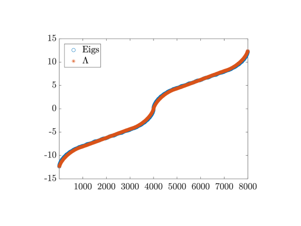
(a) Unpreconditioned

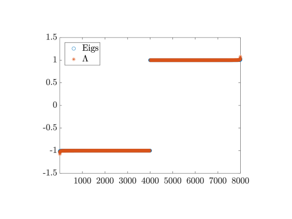
(b) $\mathcal{P}_{\boldsymbol{n}}=T_{\boldsymbol{n}}(f_{R})$

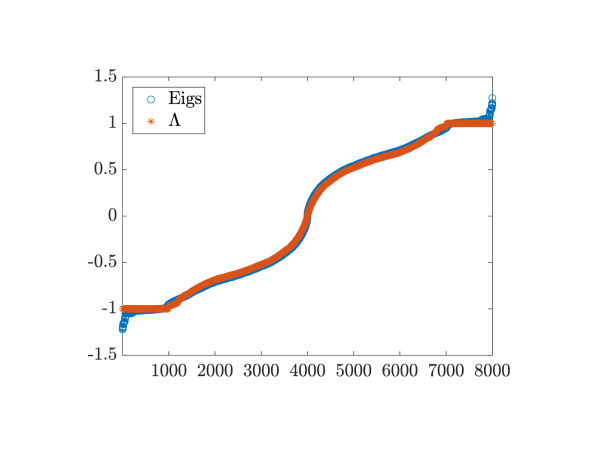
(c) $\mathcal{P}_{\boldsymbol{n}}=C_{\boldsymbol{n}}$

Figure 5: Comparison of the eigenvalues of $Y_{\boldsymbol{n}}T_{\boldsymbol{n}}$ or $\mathcal{P}_{\boldsymbol{n}}^{-1}Y_{\boldsymbol{n}}T_{\boldsymbol{n}}$ ( $\circ$) with $\Lambda$ collecting the uniform samples of the eigenvalue functions of $g$ or $h^{-1}g$ for Example 4.3 ($\ast$) $n_{1}=n_{2}=n_{3}=20$.

Table 2: Preconditioned MINRES iteration counts for Example 4.3.

$d_{\boldsymbol{n}}$	$T_{\boldsymbol{n}}(f_{R})$	$C_{\boldsymbol{n}}$
$5^{3}$	8	61
$10^{3}$	9	198
$20^{3}$	9	724

5 Conclusions

We have shown that the asymptotic eigenvalue distribution of $\{Y_{\boldsymbol{n}}T_{\boldsymbol{n}}(f)\}_{\boldsymbol{n}}$, where $T_{\boldsymbol{n}}(f)$ is a square real multilevel Toeplitz matrix generated by $f\in L^{1}([-\pi,\pi]^{d})$ and $Y_{\boldsymbol{n}}$ is the exchange matrix, is governed by a $2\times 2$ matrix-valued function whose eigenvalues are $\pm|f|$. We have also investigated the asymptotic eigenvalue distribution of preconditioned sequences $\{\mathcal{P}^{-1}_{\boldsymbol{n}}Y_{\boldsymbol{n}}T_{\boldsymbol{n}}(f)\}_{\boldsymbol{n}}$, where $\mathcal{P}_{\boldsymbol{n}}$ is Hermitian positive definite, $\{\mathcal{P}_{\boldsymbol{n}}\}_{\boldsymbol{n}}\sim_{\rm GLT}h$, and $\{\Pi_{\boldsymbol{n}}U_{\boldsymbol{n}}\mathcal{P}_{\boldsymbol{n}}U_{\boldsymbol{n}}\Pi_{\boldsymbol{n}}^{T}\}_{\boldsymbol{n}}\sim_{\rm GLT}h\cdot I_{2}$ with $h:[-\pi,\pi]^{d}\rightarrow\mathbb{C}$ and $h\neq 0$ a.e. The latter result enables us to analyse the convergence of preconditioned MINRES for this problem at least in the two quite common cases where the preconditioners are multilevel circulant or multilevel Toeplitz matrices.

References

- [1] W. M. Cheung and M. K. Ng, Block-circulant preconditioners for systems arising from discretization of the three-dimensional convection–diffusion equation, J. Comput. Appl. Math., 140 (2002), pp. 143–158, https://doi.org/10.1016/S0377-0427(01)00519-2, http://www.sciencedirect.com/science/article/pii/S0377042701005192. Int. Congress on Computational and Applied Mathematics 2000.
- [2] M. Donatelli, R. Krause, M. Mazza, and K. Trotti, Multigrid preconditioners for anisotropic space-fractional diffusion equations, Adv. in Comput. Math., 46 (2020), p. 49, https://doi.org/10.1007/s10444-020-09790-2.
- [3] H. Elman, D. Silvester, and A. Wathen, Finite Elements and Fast Iterative Solvers with Applications in Incompressible Fluid Dynamics, Oxford University Press, 2nd ed., 2014.
- [4] D. Fasino and P. Tilli, Spectral clustering properties of block multilevel Hankel matrices, Linear Algebra Appl., 306 (2000), pp. 155–163, https://doi.org/10.1016/S0024-3795(99)00251-7.
- [5] P. Ferrari, I. Furci, S. Hon, M. A. Mursaleen, and S. Serra-Capizzano, The eigenvalue distribution of special 2-by-2 block matrix-sequences with applications to the case of symmetrized Toeplitz structures, SIAM J. Matrix Anal. Appl., 40 (2019), pp. 1066–1086, https://doi.org/10.1137/18M1207399.
- [6] C. Garoni, M. Mazza, and S. Serra-Capizzano, Block generalized locally Toeplitz sequences: From the theory to the applications, Axioms, 7 (2018), p. 49, https://doi.org/10.3390/axioms7030049.
- [7] C. Garoni and S. Serra-Capizzano, Generalized locally Toeplitz sequences: theory and applications. Vol. I, Springer, Cham, 2017.
- [8] C. Garoni and S. Serra-Capizzano, Generalized locally Toeplitz sequences: a spectral analysis tool for discretized differential equations, in Splines and PDEs: From Approximation Theory to Numerical Linear Algebra, Springer, 2018, pp. 161–236.
- [9] C. Garoni and S. Serra-Capizzano, Generalized locally Toeplitz sequences: theory and applications. Vol. II, Springer, Cham, 2018.
- [10] U. Grenander and G. Szegő, Toeplitz Forms and Their Applications, vol. 321, Second Edition, Chelsea, New York, 1984.
- [11] M. Mazza and J. Pestana, Spectral properties of flipped Toeplitz matrices and related preconditioning, BIT, 59 (2019), pp. 463–482, https://doi.org/10.1007/s10543-018-0740-y.
- [12] M. Mazza, A. Ratnani, and S. Serra-Capizzano, Spectral analysis and spectral symbol for the 2d curl-curl (stabilized) operator with applications to the related iterative solutions, Math. Comput., 88 (2018), pp. 1155–1188, https://doi.org/10.1090/mcom/3366.
- [13] H. Moghaderi, M. Dehghan, M. Donatelli, and M. Mazza, Spectral analysis and multigrid preconditioners for two-dimensional space-fractional diffusion equations, J. Comput. Phys., 350 (2017), pp. 992–1011, https://doi.org/https://doi.org/10.1016/j.jcp.2017.08.064, http://www.sciencedirect.com/science/article/pii/S0021999117306459.
- [14] J. Pestana, Preconditioners for symmetrized Toeplitz and multilevel Toeplitz matrices, SIAM J. Matrix Anal. Appl., 40 (2019), pp. 870–887, https://doi.org/10.1137/18M1205406.
- [15] J. Pestana and A. J. Wathen, A preconditioned MINRES method for nonsymmetric Toeplitz matrices, SIAM J. Matrix Anal. Appl., 36 (2015), pp. 273–288, https://doi.org/10.1137/140974213.
- [16] W. Tian, H. Zhou, and W. Deng, A class of second order difference approximations for solving space fractional diffusion equations, Math. Comp., 84 (2015), pp. 1703–1727, https://doi.org/10.1090/S0025-5718-2015-02917-2.
- [17] P. Tilli, A note on the spectral distribution of Toeplitz matrices, Linear Multilin. Algebra, 45 (1998), pp. 147–159, https://doi.org/10.1080/03081089808818584.
- [18] N. L. Zamarashkin and E. E. Tyrtyshnikov, Distribution of eigenvalues and singular values of Toeplitz matrices under weakened conditions on the generating function, Sbornik: Mathematics, 188 (1997), p. 1191, https://doi.org/10.1070/SM1997v188n08ABEH000251.