Real-Time Radio Technology and Modulation Classification via an LSTM Auto-Encoder

Abstract

Identification of the type of communication technology and/or modulation scheme based on detected radio signal are challenging problems encountered in a variety of applications including spectrum allocation and radio interference mitigation. They are rendered difficult due to a growing number of emitter types and varied effects of real-world channels upon the radio signal. Existing spectrum monitoring techniques are capable of acquiring massive amounts of radio and real-time spectrum data using compact sensors deployed in a variety of settings. However, state-of-the-art methods that use such data to classify emitter types and detect communication schemes struggle to achieve required levels of accuracy at a computational efficiency that would allow their implementation on low-cost computational platforms. In this paper, we present a learning framework based on an LSTM denoising auto-encoder designed to automatically extract stable and robust features from noisy radio signals, and infer modulation or technology type using the learned features. The algorithm utilizes a compact neural network architecture readily implemented on a low-cost computational platform while exceeding state-of-the-art accuracy. Results on realistic synthetic as well as over-the-air radio data demonstrate that the proposed framework reliably and efficiently classifies received radio signals, often demonstrating superior performance compared to state-of-the-art methods.

I Introduction

Analysis of detected radio signals enables classification of communication technology and modulation schemes employed by the source that emitted the signals; this information helps optimize spectrum allocation and mitigate radio interference, supports wireless environment analysis and enables improvement of communication efficiency. However, increase in the numbers of emitter types and sources of interference, as well as temporal variations in the effects of wireless environment on the transmitted signals, render the accurate inference of communication schemes and emitter types computationally challenging.

Existing methods for modulation and technology classification can be organized into two sub-groups, likelihood-based and feature-based [1]. Likelihood-based methods make a decision by evaluating a likelihood function of the received signal and comparing the likelihood ratio with a pre-defined threshold. Although the likelihood-based classifiers are optimal in that they minimize the probability of false classification, they suffer from high computational complexity [1]. On the other hand, feature-based approaches are relatively simple to implement and may achieve near-optimal performance but the features and decision criteria need to be carefully designed. Such methods rely on expert features including cyclic moments [2] and their variations [3], and spectral correlation functions of analog and digital modulated signals [4, 5]; [6] describes novel decision criteria which utilize pre-existing expert features. [7] facilitates classification via a multilayer perceptron that relies on spectral correlation functions. Expert systems have been shown to achieve high accuracy on certain special tasks but may be challenging to apply in general settings since the crafted features may not fully reflect all the real-world channel effects. As an alternative, deep learning based methods that learn directly from the received signals have recently been proposed. In particular, [8] utilizes a convolutional neural network (CNN) that operates on in-phase and quadrature-phase (IQ) data and outperforms expert features based methods. [9] combines CNN and long short-term memory (LSTM) [10, 11] to further improve classification accuracy. [12] utilizes an LSTM on amplitude and phase data by simply transferring IQ data for modulation classification, outperforming the proposed model in [9]. [13] proposes two classification models with one adapting the Visual Geometry Group (VGG) architecture [14] principles to a 1D CNN and the other utilizing the ideas of deep residual networks (RNs) [15]. Note that while spectrum monitoring devices are capable of acquiring detailed wireless signal’s IQ components, storage of such data on distributed sensing devices or their transmission to a cloud or edge device for processing is often infeasible due to resource constraints. To this end, distributed spectrum monitoring systems such as Electrosense [16] formulate technology detection task as the classification that uses more compact Power Spectral Density (PSD) data as features. Note, however, that the aforementioned deep learning architectures are infeasible for use in distributed settings and on low-cost computational platforms. More details on practical aspects of RF acquisition can be found in [17].

In this paper, we propose a new learning framework for both modulation as well as technology classification problems based on an LSTM denoising auto-encoder. The framework aims to estimate posterior probabilities of the modulation or technology types using time domain amplitude and phase of a radio signal. Auto-encoders in an unsupervised manner learn a low-dimensional representation of data; more specifically, they attempt to perform a dimensionality reduction while robustly capturing essential content of high-dimensional data [18]. Typically, auto-encoders consist of two blocks: an encoder and a decoder. The encoder converts input data into the so-called codes while the decoder reconstructs the input from the codes. The act of copying the input data to the output would be of little interest without an important additional constraint – namely, the constraint that the dimension of codes is smaller than the dimension of the input. This enables auto-encoders to extract salient features of the input data. A denoising auto-encoder (DAE) [19] can help extract stable and robust features by introduction noise corruption to the input signal. In our proposed framework, the received radio signals are first partially corrupted and the framework then recovers the destroyed signals, simultaneously learning stable and robust low-dimensional signal representations and classifying the signals based on the learned features.

Our main contributions are summarized as follows:

• We propose a new learning framework which uses amplitude and phase data for modulation classification; the framework is based on an LSTM denoising auto-encoder and achieves state-of-the-art modulation classification accuracy.

• We extend the proposed framework to technology classification using power spectral density data.

• The proposed framework achieves significantly higher top-1 classification accuracy while having much simpler structure than the existing models. This enables real-time modulation and/or technology classification on compact and affordable computational devices, as we demonstrate using Raspberry PI platforms.

II Methods

II-A Problem Formulation

Let $r_{t_{i}}=(x_{1},...,x_{n})$ denote a sequence of $m$-dimensional features characterizing $n$ samples of the received radio signal sampled starting at time $t_{i}$. The goal of modulation (technology) classification is to identify the modulation (technology) type of the radio signal among $K$-classes by estimating $P(y=C_{k}|r_{t_{i}})$ where $C_{k}$ denotes the $k^{th}$ class and $y$ is the true class of the signal.

For modulation classification, the features are the IQ components of the sampled signal (i.e., $m=2$). Figure 1 shows examples of the IQ components for 11 different modulation types found in RadioML2016.10A dataset for signal-to-noise ratio (SNR) of $10$dB. Although there are differences between the IQ components, it is challenging even for a domain expert to distinguish between them due to pulse shaping, distortion and other channel effects [8].

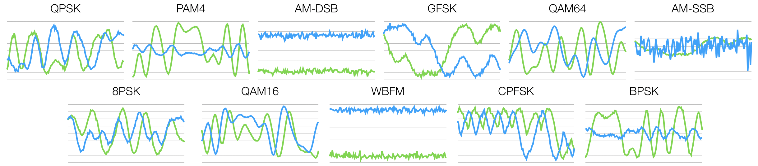
Figure 1: IQ component examples of 11 different modulation types from RadioML2016.10A data with $SNR=10$dB. The x-axis represents time and the y-axis represents amplitude. The blue line shows the in-phase component while the green line shows the quadrature component.

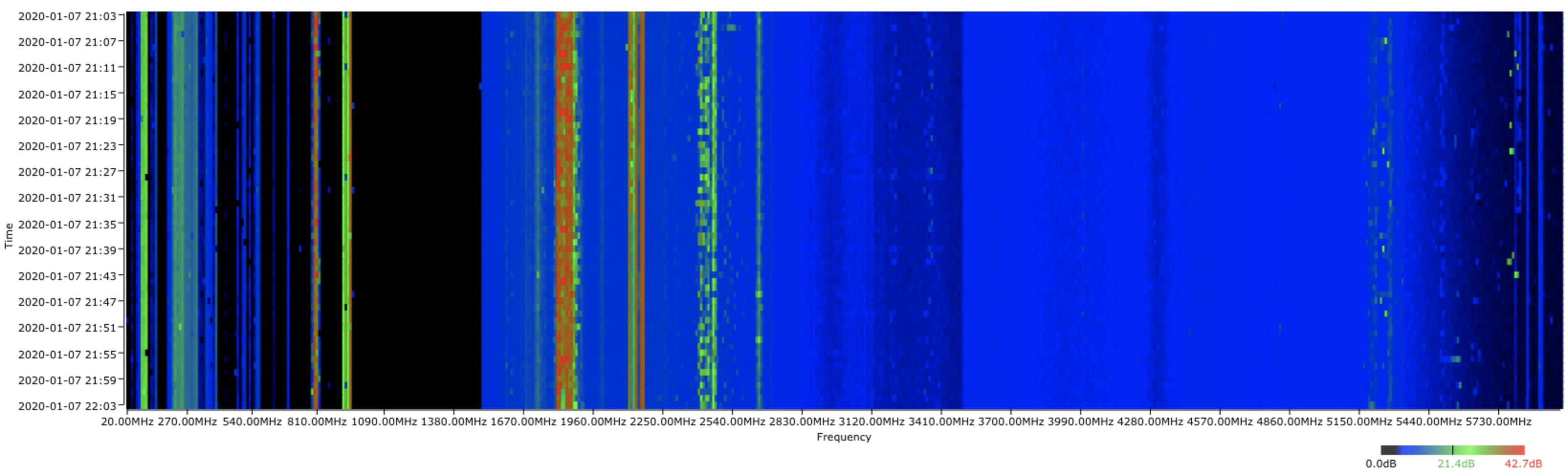
Figure 2: The wireless magnitude spectrum collected by one of the Electrosense sensors. The x-axis contains different centre frequencies while the y-axis shows sampling times.

For technology classification, the spectrum of interest is scanned by selecting a candidate carrier frequency $f_{j}$ in discrete increments, and for each such frequency a fast Fourier transform (FFT) of the received signal demodulated into baseband is computed. Average values of the FFT coefficients computed for each $f_{j}$ are then concatenated to form a sequence of features used to perform the classification task. For the Electrosense data that we analyze in this paper, $f_{j}\in(50\text{MHz},6\text{GHz})$ and the scanning resolution is $0.1$MHz. Figure 2 shows an example of wireless magnitude spectrum data from one of the Electrosense sensors.

To characterize the performance of modulation and technology classification methods, we rely on top-1 classification accuracy over SNR, confusion matrix, time and space complexity in terms of the number of trainable parameters and model size, and testing time on Raspberry Pi.

II-B An LSTM Denoising Auto-Encoder

In this section, we describe the design of our proposed classifier based on a denoising auto-encoder and recurrent neural networks. Instead of using IQ components, for modulation classification we rely on L2-normalized amplitude and normalized phase (falling between -1 and 1, in radians); such normalization benefits learning temporal dependencies [12].

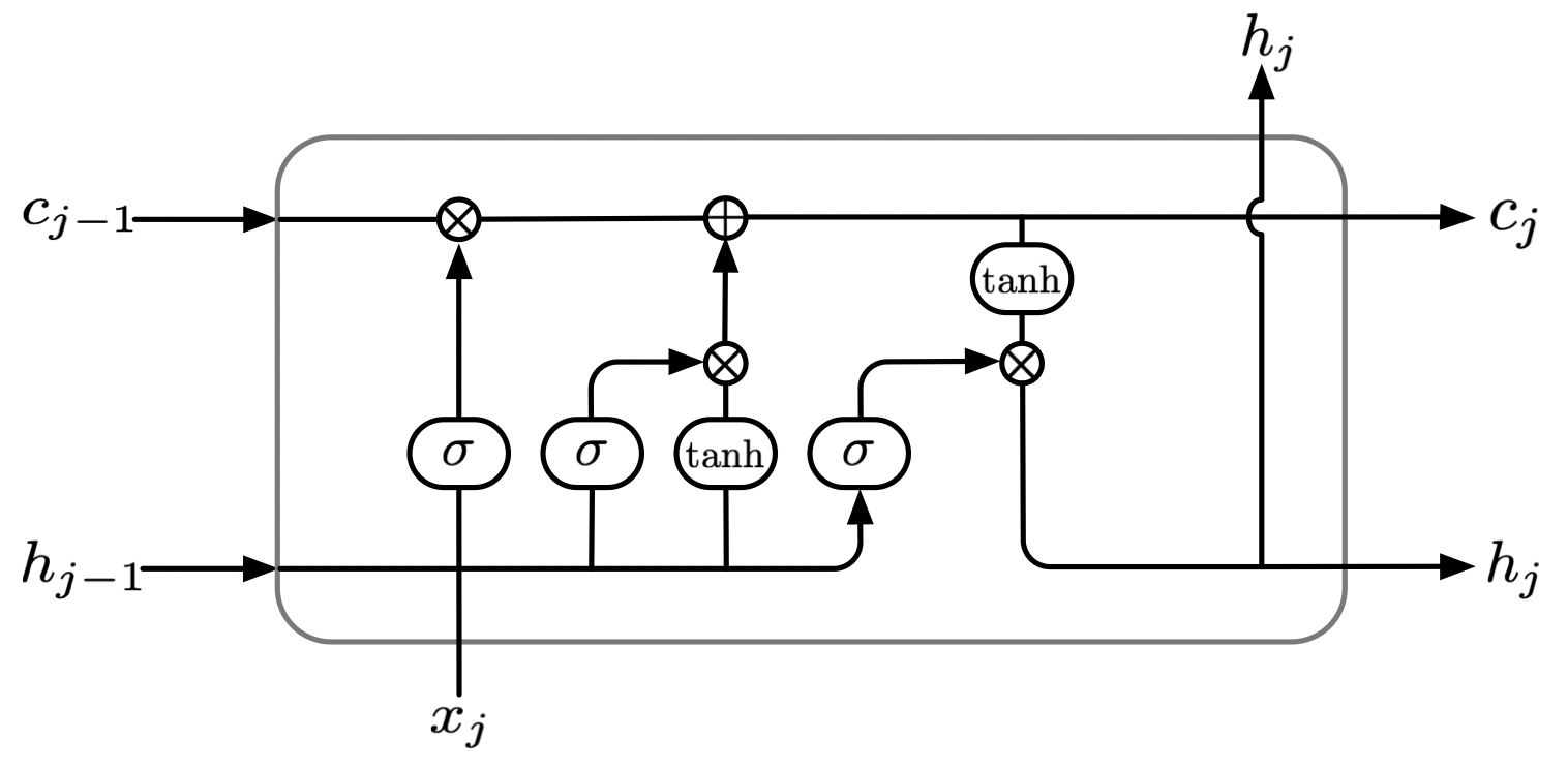
Figure 3: Structure of an LSTM cell.

A sampled radio signal results in a time series, and an LSTM is utilized to efficiently capture temporal structure of such a series. Figure 3 shows the structure of an LSTM cell with a forget gate. The input gate, output gate and forget gate can be expressed respectively as

$$i_{j}=\sigma(W_{i}x_{j}+U_{i}h_{j-1}+b_{i}),$$ (1)

$$o_{j}=\sigma(W_{o}x_{j}+U_{o}h_{j-1}+b_{o}),$$ (2)

and

$$f_{j}=\sigma(W_{f}x_{j}+U_{f}h_{j-1}+b_{f}),$$ (3)

while the cell state vector and hidden state vector are defined as

$$c_{j}=f_{t}\cdot c_{j-1}+i_{j}\cdot\tanh(W_{c}x_{j}+U_{c}h_{j-1}+b_{c})$$ (4)

and

$$h_{j}=o_{j}\cdot\tanh(c_{j}),$$ (5)

respectively, where $\sigma$ denotes the sigmoid function (i.e., $\sigma(z)=\frac{1}{1+e^{-z}}$), $W$ denotes a weight matrix for the input time series, $U$ is a weight matrix for the hidden state vector, and $b$ represents a bias vector.

The denoising auto-encoder corrupts the signal by randomly setting a portion of samples of $r(t)$ to $0$, thus obtaining a partially destroyed signal $\tilde{r}_{(t)}=(\tilde{x}_{1},...,\tilde{x}_{n})$. The partially destroyed signal is fed to the auto-encoder for training while the original signal is utilized for testing.

Motivated by [19], [20] and [21], we propose a novel LSTM denoising auto-encoder for modulation/technology classification where the auto-encoder and classifier are trained simultaneously.

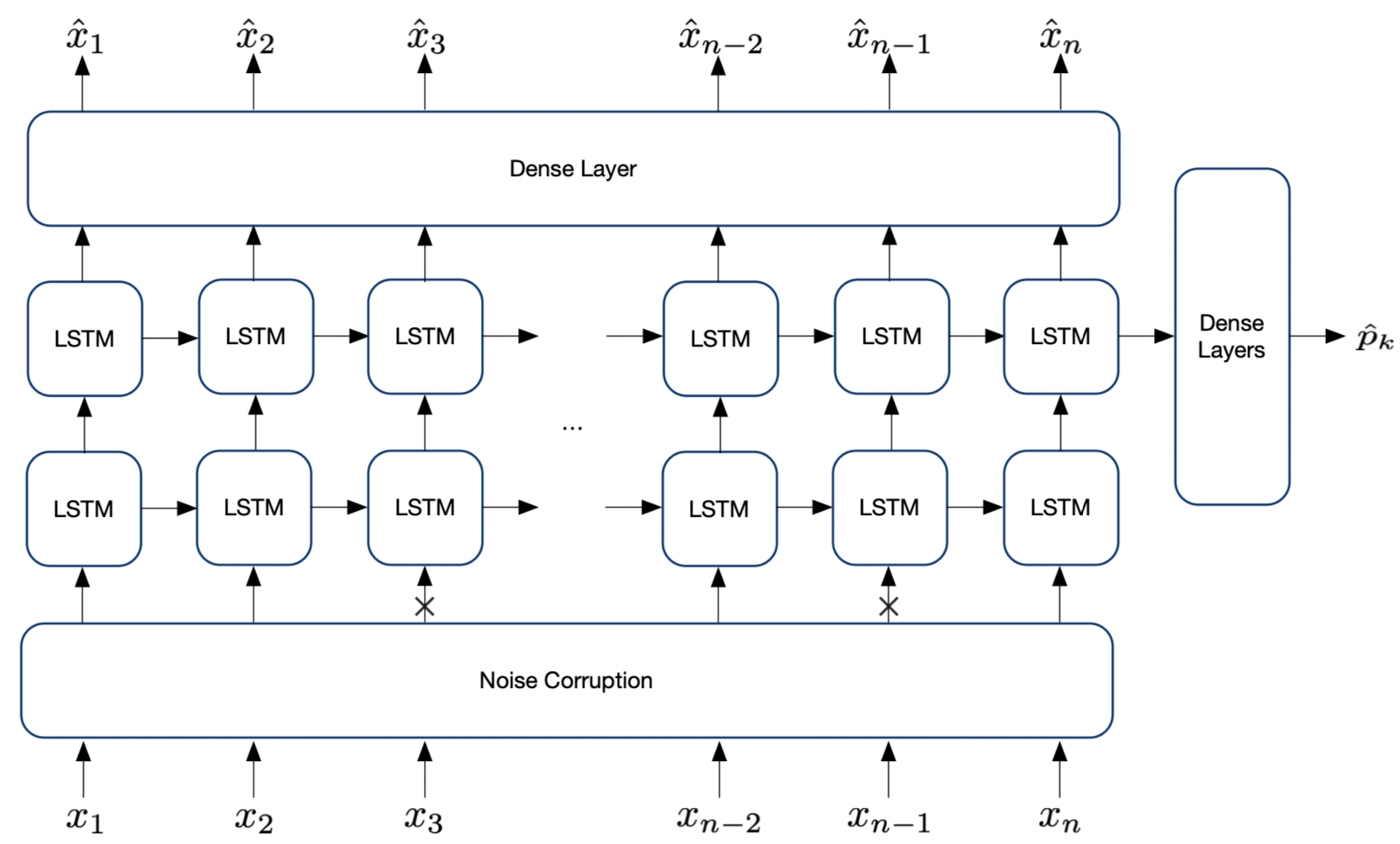
Figure 4: An LSTM denoising auto-encoder classifier.

Figure 4 shows the LSTM denoising auto-encoder classifier. The classifier is connected to the last hidden state vector $h_{n}$ and it consists of 3 fully connected layers followed by a softmax function, i.e.,

$$o^{\text{clf}}_{(1)}=\sigma(W^{\text{clf}}_{(1)}h_{n}+b^{\text{clf}}_{(1)}),$$ (6)

$$o^{\text{clf}}_{(2)}=\sigma(W^{\text{clf}}_{(2)}o^{\text{clf}}_{(1)}+b^{\text{clf}}_{(2)}),$$ (7)

$$o^{\text{clf}}_{(3)}=\sigma(W^{\text{clf}}_{(3)}o^{\text{clf}}_{(2)}+b^{\text{clf}}_{(3)}),$$ (8)

$$\hat{p}_{k}=\frac{e^{o^{\text{clf}}_{(3)_{k}}}}{\sum_{k=1}^{K}e^{o^{\text{clf}}_{(3)_{k}}}},$$ (9)

where $W^{\text{clf}}$ denotes the weight matrix, $b^{\text{clf}}$ is the bias vector, $o^{\text{clf}}$ denotes the output of a fully connected layer for classification ($o^{\text{clf}}_{(3)_{k}}$ represents its $k^{th}$ entry), $\hat{p}_{k}$ denotes the probability of predicting $r(t)$ as the $k^{th}$ class and $\sigma$ denotes the rectified linear unit (ReLU). The 2-layer LSTM operates as an encoder that converts the corrupted input $\tilde{r}_{(t)}$ into hidden state vectors $(h_{1},...,h_{n})$ while a shared fully connected layer operate as a decoder, i.e.,

$$\hat{x}_{j}=W^{\text{dec}}h_{j}+b^{\text{dec}},$$ (10)

where $\hat{x}_{j}$ is the $j^{th}$ recovered sample, $W^{\text{dec}}$ denotes the weight matrix of the decoder and $b^{\text{dec}}$ is the bias vector for the fully connected layer. Note that we break the symmetry of the architecture by using a shared fully connected layer for the decoder since doing so reduces computational complexity.

Therefore, the loss function of the network consists of the reconstruction loss, $L_{\text{DAE}}$, and the classification loss, $L_{\text{clf}}$. The final loss function is a weighted combination of these two terms, i.e.,

$$L=(1-\lambda)L_{\text{DAE}}+\lambda L_{\text{clf}},$$ (11)

where $\lambda\in[0,1]$ is a hyperparameter balancing $L_{\text{DAE}}$ and $L_{\text{clf}}$. It is worth pointing out that a small $\lambda$ eliminates the effects of classification layers while a large $\lambda$ distorts the learned representation of data. We set the value of $\lambda$ to 0.1 to promote extraction of reliable low-dimensional representations of the original signals and thus enable efficient classification with reduced dimensionality of the hidden state of an LSTM cell. This allows the proposed model to achieve higher classification accuracy at a significantly reduced computational complexity. The reconstruction loss $L_{\text{DAE}}$ is defined to be the mean-squared error (MSE) and can be expressed as

$$L_{\text{DAE}}=\frac{1}{n}\sum_{j=1}^{n}(x_{j}-\hat{x}_{j})^{2},$$ (12)

while the classification loss $L_{\text{clf}}$ is defined to be the categorical cross entropy

$$L_{\text{clf}}=-\sum_{k=1}^{K}p_{k}\log\hat{p}_{k},$$ (13)

where $p_{k}=1$ if $r(t)$ belongs to the $k^{th}$ class and $p_{k}=0$ otherwise.

II-C Model Parameters

For both tasks, we rely on Adam optimizer [22] since it helps avoid local optima. The dimensionality of the hidden states of the LSTM in our denoising autoencoder is set to $32$. Please note that prior LSTM-based methods require more than 128 hidden states to achieve desired level of accuracy; otherwise, the classification accuracy deteriorates significantly as shown in [12]. The number of nodes in the dense layer of decoder is set to $m$ and the number of nodes in the fully connected layers of the classifier are set to $32$, $16$ and $K$, respectively. The learning rate is set to $0.001$ and the number of epochs is set to $150$. Dropout rate is chosen to be $0.2$ for the LSTMs and fully connected layers; randomly selected 10% of the entries of the input signal in the training data are masked by $0$. The models are implemented on a computer with 3.70GHz Intel i7-8700K processor, 2 NVIDIA GeForce GTX 1080Ti computer graphics cards and 32GB of RAM. The minibatch size of 128 is utilized. The parameter $\lambda$ controlling how the reconstruction loss and classification loss are combined is set to $0.1$.

III Results

III-A Performance Comparison on RadioML2016.10A

We first evaluate performance of the proposed model for modulation classification on a realistic RadioML2016.10A dataset. RadioML data includes a series of synthetic and over-the-air modulation classification sets created by DeepSig Inc. Among them, RadioML2016.10A has in particular been widely used for benchmark testing [23, 9, 12]. Radio channel effects including time-delay, time-scaling, phase rotation, frequency offset and additive thermal noise are accounted for to emulate practical radio communications (details can be found in [24]). The set contains data for 11 modulation schemes (8PSK, AM-DSB, AM-SSB, BPSK, CPFSK, GFSK, PAM4, QAM16, QAM64, QPSK and WBFM). The SNR ranges from -20dB to 18dB with 2dB step size; there are $1000$ samples for each SNR resulting in the total of 220k samples. The sample length is 128. We used 50%, 25% and 25% of the dataset for training, validation and testing, respectively.

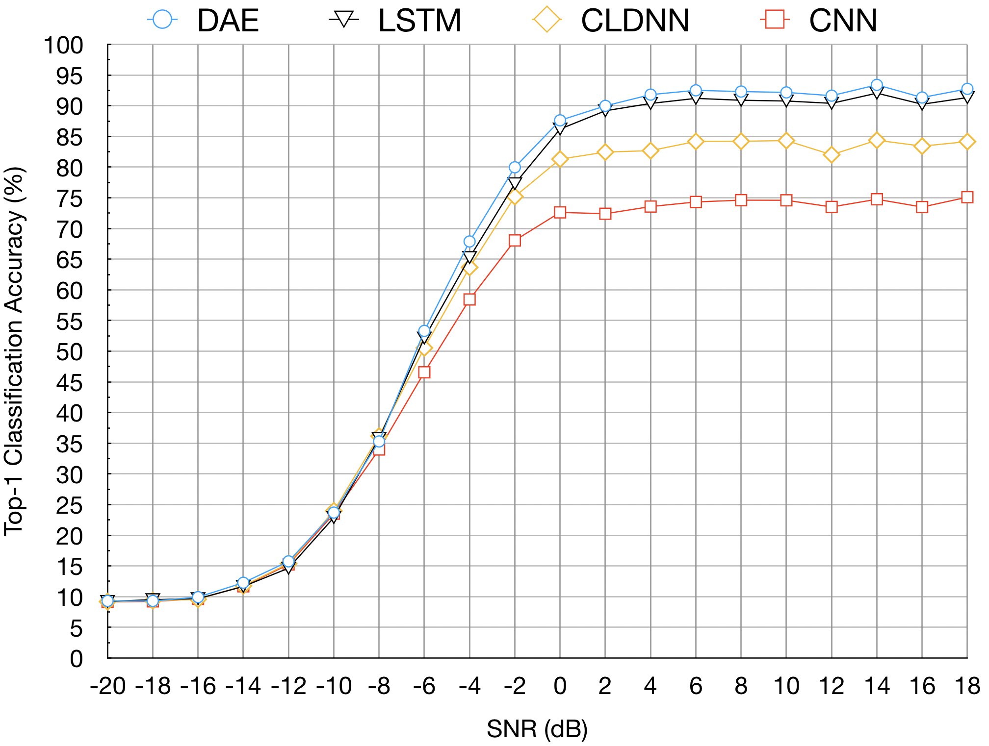
Figure 5: Top-1 classification accuracy of our proposed model (DAE) vs. existing models on RadioML2016.10A dataset.

TABLE I: Top-1 classification accuracy comparison of our proposed model (DAE) vs. existing models on RadioML2016.10A dataset. The highest average top-1 classification accuracy for each SNR is marked in bold.

Model		-20dB	-18dB	-16dB	-14dB	-12dB	-10dB	-8dB
DAE	Mean	9.30	9.35	9.92	12.27	15.75	23.70	35.29
	Std	0.09	0.17	0.43	0.98	1.32	1.25	1.13
LSTM	Mean	9.22	9.51	9.67	11.66	14.64	22.89	35.78
	Std	0.21	0.23	0.30	0.62	1.11	1.31	1.31
CLDNN	Mean	9.19	9.35	9.56	11.76	15.39	23.98	36.16
	Std	0.16	0.22	0.23	0.74	1.17	1.38	1.61
CNN	Mean	9.15	9.23	9.64	11.68	15.24	23.51	33.98
	Std	0.13	0.26	0.40	0.79	0.98	1.31	0.82

Model		-6dB	-4dB	-2dB	0dB	2dB	4dB	6dB
DAE	Mean	53.31	67.88	79.97	87.62	89.98	91.81	92.61
	Std	1.56	1.23	1.08	0.74	0.60	0.45	0.23
LSTM	Mean	52.14	65.26	77.29	86.20	89.18	90.37	91.20
	Std	0.94	1.07	0.65	0.85	0.64	0.81	0.52
CLDNN	Mean	50.54	63.66	75.20	81.30	82.45	82.68	84.18
	Std	1.30	1.57	1.53	0.83	0.91	1.43	0.96
CNN	Mean	46.56	58.43	68.05	72.62	72.40	73.57	74.32
	Std	1.06	0.92	0.65	1.14	0.91	1.56	1.15

Model		8dB	10dB	12dB	14dB	16dB	18dB	Overall
DAE	Mean	92.31	92.17	91.64	93.40	91.34	92.75	61.72
	Std	0.31	0.34	0.46	0.31	0.17	0.31	0.18
LSTM	Mean	90.89	90.77	90.39	92.05	90.24	91.33	60.49
	Std	0.50	0.58	0.78	0.63	0.69	0.78	0.37
CLDNN	Mean	84.21	84.32	82.02	84.38	83.41	84.16	56.78
	Std	1.14	0.82	0.90	0.79	1.02	0.99	0.46
CNN	Mean	74.61	74.59	73.51	74.76	73.49	75.10	51.29
	Std	0.97	1.31	1.33	1.29	1.60	1.54	0.40

The two-layer LSTM denoising auto-encoder is trained on SNRs ranging from -20dB to 18dB. The top-1 classification accuracy of CNN [8], CLDNN [9], LSTM [12] and our proposed model is shown in Figure 5 and Table I. The classification accuracy computed over all SNRs achieved by CNN, CLDNN, LSTM and our proposed model is 51.29%, 56.78%, 60.49% and 61.72%, respectively. It is worth pointing out that training with noise helps increase the classification accuracy (computed across all SNRs) by 1.1% as compared to training with the original signal. The auto-encoder enables extraction of stable low-dimensional features with a significantly reduced dimension of hidden LSTM states and thus contributes to the improvement in classification accuracy and the reduction of computational complexity. The average classification accuracy for SNRs ranging from 0dB to 18dB achieved by CNN, CLDNN, LSTM and our proposed model is 73.9%, 83.31%, 90.26% and 91.55%, respectively. The proposed model outperforms selected models for almost all SNRs. The considered softwares were executed with their default settings, i.e., we use the same hyperparameters as the authors of existing methods did when running their methods on RadioML10.A dataset. The results in Figure 5 are averaged over 10 experiments. Model parameters were initialized at the beginning of each experiment. Note that the benchmarking results for the pre-existing methods that we obtained closely match those reported in [12]. It is worth pointing out that our proposed model significantly outperforms CLDNN and CNN in high SNR regimes, while marginally outperforming LSTM in terms of top-1 classification accuracy. Figure 6-8 illustrate the confusion matrices in the experiment that achieved the highest overall top-1 classification accuracy for the proposed model and LSTM for SNRs 18dB, 0dB and -4dB. For the SNR of 18dB, the diagonal is much more sharp even though there are some confusions in separating AM-DSB from WBFM signals, which are mainly due to the silence periods of audio [12]. Similar to Figure 7, there are some difficulties in separating AM-DSB and WBFM at the SNR of 0dB. Besides, there is some level of confusion between QAM16 and QAM64 since QAM16 is a subset of QAM64. It is also worth mentioning that the proposed model performs better on AM-SSB signals and on distinguishing QAM64 from QAM16 signals at high SNRs. As shown in Figure 8, it becomes much more difficult to distinguish the signals at low SNRs.

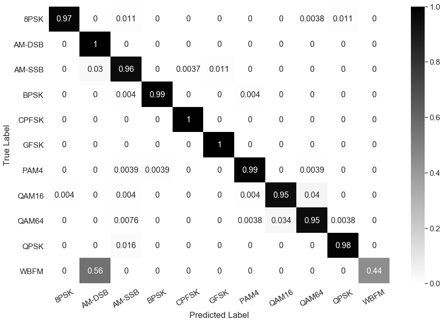
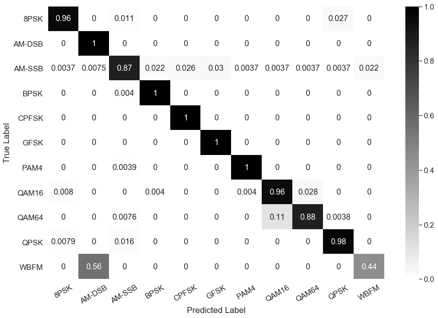
Figure 6: Confusion matrix for the proposed model (top) and LSTM (bottom) on RadioML2016.10A dataset at 18dB SNR.

Figure 7: Confusion matrix for the proposed model (top) and LSTM (bottom) on RadioML2016.10A dataset at 0dB SNR.

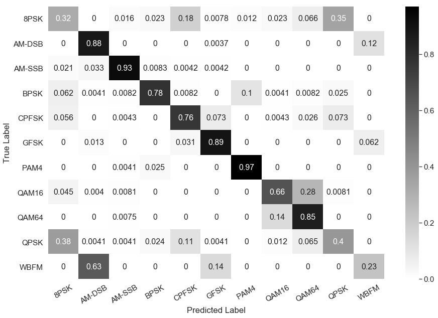
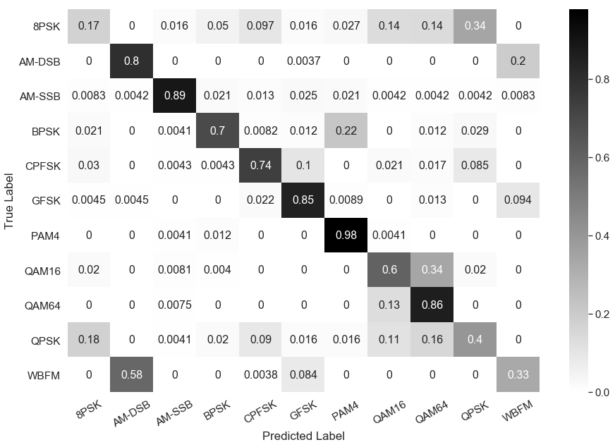
Figure 8: Confusion matrix for the proposed model (top) and LSTM (bottom) on RadioML2016.10A dataset at -4dB SNR.

TABLE II: A comparison of the number of trainable parameters, FLOPs and memory cost on RadioML2016.10A data.

Model	# Parameters	# FLOPs	Memory
DAE	14637	45040	224KB
LSTM	200075	660239	2.32MB
CLDNN	248817	588974	2.91MB
CNN	5456219	80548043	61.4MB

TABLE III: Number of classifications per second on different platforms on RadioML2016.10A data.

Platform		DAE	LSTM	CLDNN	CNN
GTX 1080Ti	Mean	8456	7325	10257	19162
	Std	153.97	138.72	102.28	346.64
Intel i7-8700K	Mean	1255	869	871	1578
	Std	7.72	21.62	15.70	14.36
Raspberry Pi 4	Mean	241	42	45	127
	Std	14.61	0.51	1.36	1.01
Raspberry Pi 3	Mean	119	19	20	45
	Std	1.45	1.97	0.23	2.39

Next, we compare considered models in terms of the number of trainable parameters, the number of floating point operations (FLOPs), the memory cost, and the number of classifications per second on different computational platforms. As shown in Table II, the proposed model has the smallest number of trainable parameters and requires the fewest FLOPs and the smallest memory space. Table III shows that in terms of the number of classifications per second on Raspberry Pi 4, the proposed model is on average approximately $5.6\times$, $5.4\times$ and $1.9\times$ faster than LSTM, CLDNN and CNN, respectively. On Raspberry Pi 3, the proposed model is on average approximately $6.3\times$, $6\times$ and $2.6\times$ faster than LSTM, CLDNN and CNN, respectively. The mean and standard deviation of the number of classifications per second are averaged over 10 experiments. Note that the complexity of existing methods cannot be reduced without causing severe deterioration of classification accuracy [12].

III-B Performance Comparison on RadioML2018.01A

We next evaluate performance of the proposed model on the modulation classification task using the realistic over-the-air RadioML2018.01A data with specific radio channel effect settings including carrier frequency offset, symbol rate offset, delay spread and thermal noise [13]. Signals over the so-called Normal Classes that are commonly seen in impaired environments, including OOK, 4ASK, BPSK, QPSK, 8PSK, 16QAM, AM-SSB-SC, AM-DSB-SC, FM, GMSK and OQPSK, are utilized. The data contains 11 modulations and the SNR range is from -20dB to 30dB with 2dB step size. For each SNR and modulation scheme there are 4096 samples, leading to about 1.17M samples in total. The sample length is 1024 and each sample is composed of IQ components. 50%, 25% and 25% of the entire dataset are used for training, validation and testing, respectively.

Table IV shows the mean and standard deviation of top-1 classification accuracy over the range of SNRs for a number of models computed over 10 experiments. The classification accuracy computed over all SNRs achieved by VGG, RN and our proposed model is 64.03%, 66.00% and 67.30%, respectively. Note that training with noise helps increase the classification accuracy (computed across all SNRs) by 0.9% as compared to training with the original signal. As before, the auto-encoder enables extraction of stable low-dimensional features with a significantly reduced dimension of hidden LSTM states, hence contributing to the improvement in classification accuracy and the reduction of computational complexity. The classification accuracy over the range of SNR from $0$dB to $30$dB achieved by VGG, RN and our proposed model is 92.16%, 94.89% and 96.56%, respectively. The proposed model outperforms state-of-the-art models for almost all SNRs.

The top-1 classification accuracy of the VGG and residual networks (RN) used in [13] and the proposed model across different SNRs are shown in Figure 9. Results in Figure 9 are averaged over 10 experiments.

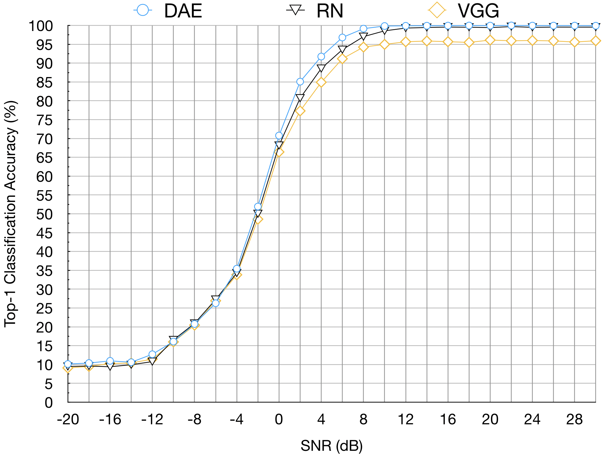
Figure 9: Top-1 classification accuracy comparison of the proposed model (DAE) with selected models on RadioML2018.01A dataset.

Figure 10-12 illustrate the confusion matrices for the experiment with the highest overall top-1 classification accuracy for the proposed model and LSTM at the SNRs 18dB, 6dB and 0dB. For the SNR of 18dB, the diagonal is very sharp for the proposed model while there are some confusions between AM-SSB-SC and 4ASK signals for RN and VGG. At the SNR of 0dB, it becomes more difficult for the proposed model to separate AM-SSB-SC and 4ASK. As shown in Figure 12, it becomes much more difficult to distinguish the signals at low SNRs and all considered models start making mistakes differentiating between GMSK, OQPSK and BPSK signals.

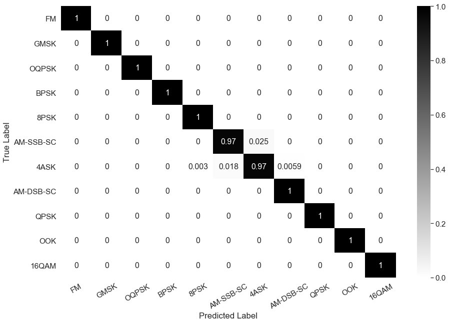
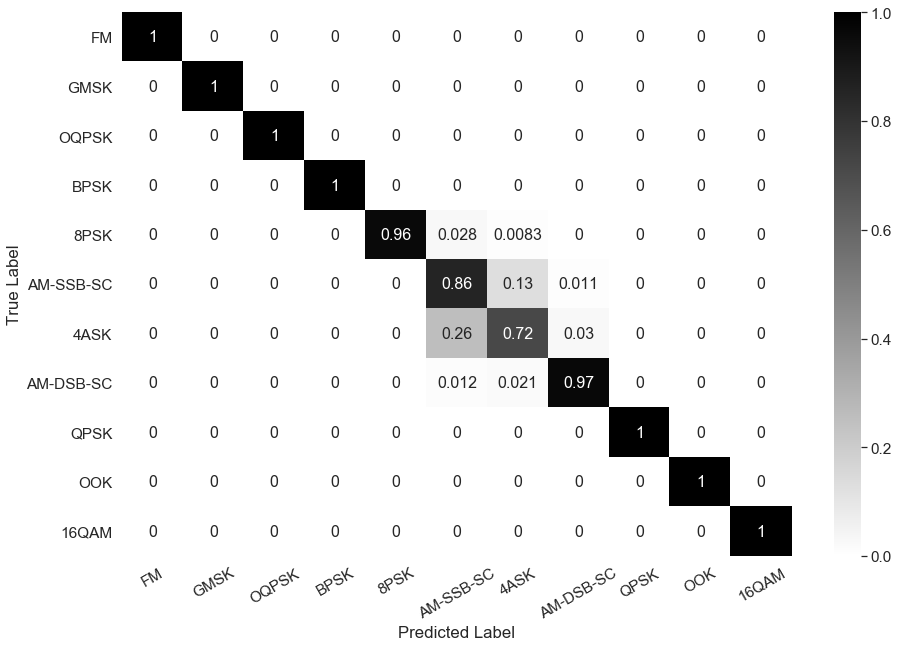
Figure 10: Confusion matrix for the proposed model (top), RN (middle) and VGG (bottom) on RadioML2018.01A dataset at 18dB SNR.

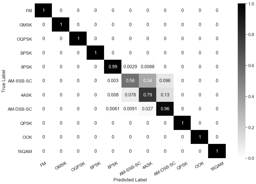
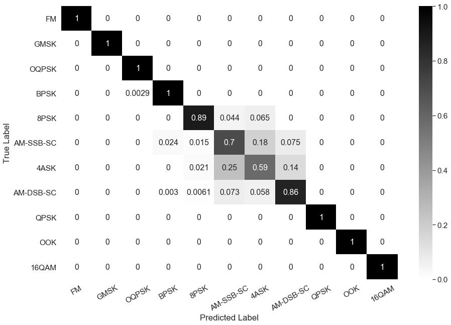
Figure 11: Confusion matrix for the proposed model (top), RN (middle) and VGG (bottom) on RadioML2018.01A dataset at 6dB SNR.

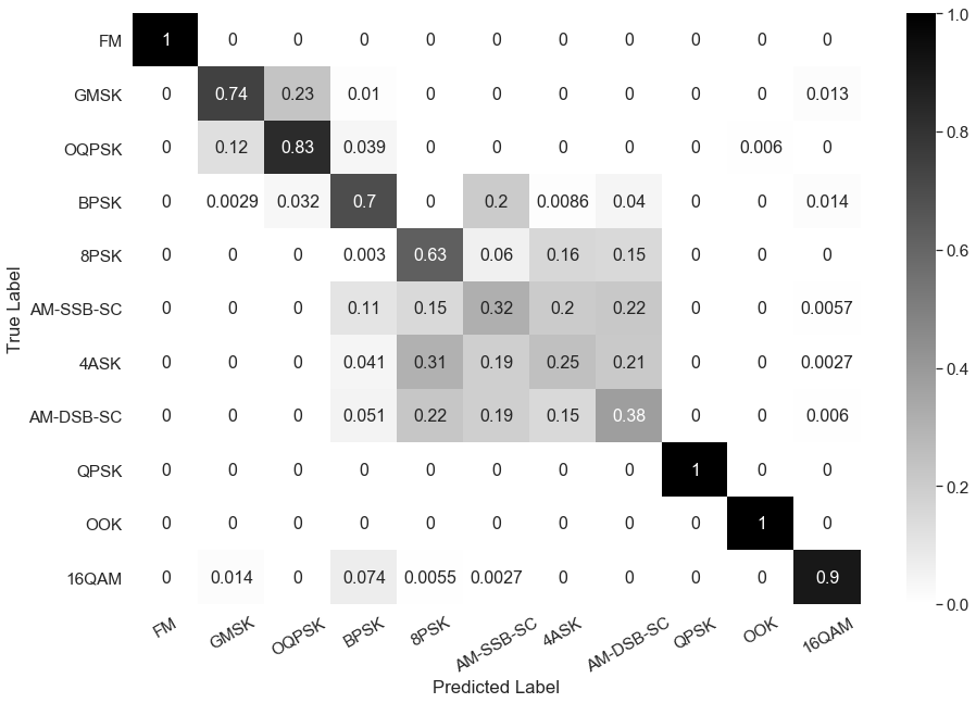
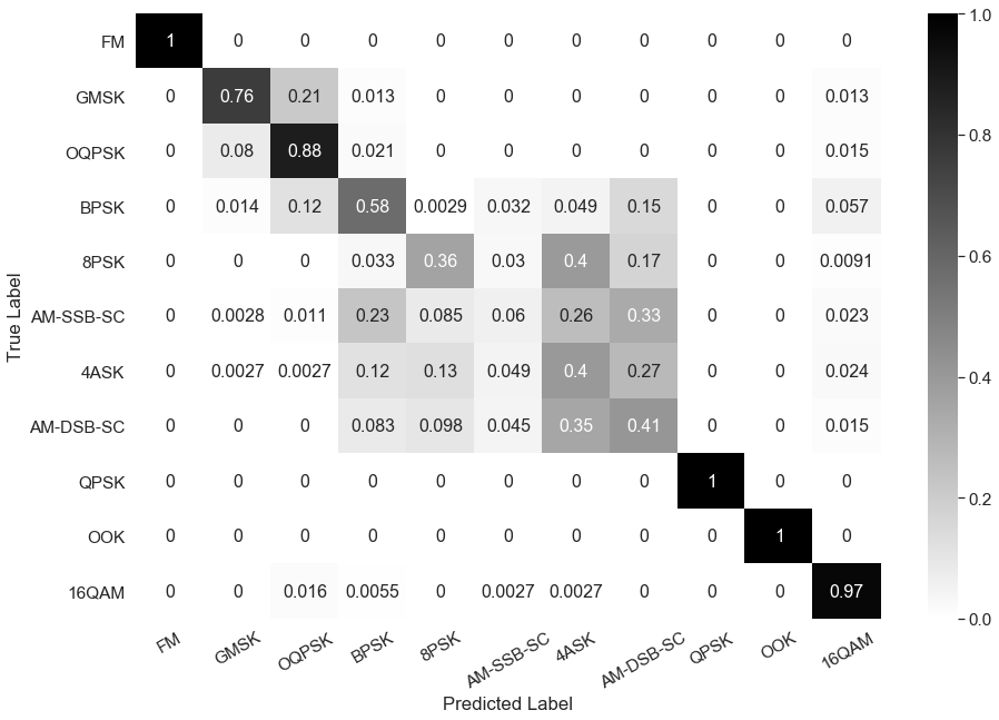
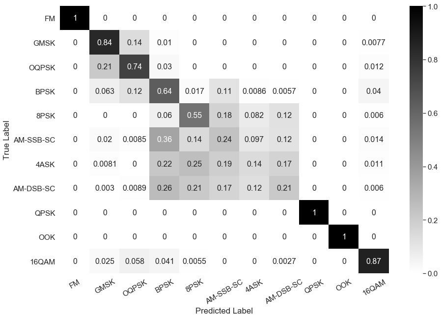
Figure 12: Confusion matrix for the proposed model (top), RN (middle) and VGG (bottom) on RadioML2018.01A dataset at 0dB SNR.

TABLE IV: Top-1 classification accuracy comparison of the proposed model (DAE) vs. existing models on RadioML2018.01A dataset (mean and standard deviation). The highest average top-1 classification accuracy for each SNR is marked in bold.

Model		-20dB	-18dB	-16dB	-14dB	-12dB	-10dB	-8dB
DAE	Mean	9.86	9.73	10.03	11.05	12.84	17.33	20.43
	Std	0.32	0.32	0.40	0.48	0.42	0.46	0.43
RN	Mean	9.28	9.42	9.69	10.49	11.81	16.21	19.87
	Std	0.50	0.60	0.46	0.43	0.89	0.77	0.87
VGG	Mean	9.82	9.17	9.69	10.59	11.50	15.41	19.87
	Std	0.47	0.40	0.38	0.41	0.48	0.67	0.39

Model		-6dB	-4dB	-2dB	0dB	2dB	4dB	6dB
DAE	Mean	26.71	35.84	52.41	72.04	85.31	92.10	97.19
	Std	0.32	0.43	0.51	0.26	0.32	0.38	0.16
RN	Mean	26.54	34.33	50.34	68.65	80.90	87.88	93.54
	Std	1.35	0.95	0.98	1.21	0.72	0.69	0.50
VGG	Mean	27.69	34.57	47.91	65.43	78.04	85.29	91.25
	Std	0.46	0.66	0.82	0.65	0.62	0.56	0.20

Model		8dB	10dB	12dB	14dB	16dB	18dB	20dB
DAE	Mean	99.33	99.77	99.91	99.87	99.95	99.95	99.91
	Std	0.09	0.05	0.05	0.05	0.05	0.08	0.05
RN	Mean	97.26	98.29	98.81	99.12	99.26	99.24	99.28
	Std	0.28	0.41	0.50	0.29	0.32	0.37	0.30
VGG	Mean	94.07	94.75	95.80	95.89	96.10	95.70	96.22
	Std	0.23	0.31	0.32	0.38	0.34	0.29	0.24

Model		22dB	24dB	26dB	28dB	30dB	Overall
DAE	Mean	99.94	99.97	99.95	99.91	99.93	67.30
	Std	0.01	0.03	0.06	0.04	0.02	0.17
RN	Mean	99.21	99.17	99.22	99.15	99.28	66.00
	Std	0.38	0.39	0.35	0.36	0.40	0.22
VGG	Mean	96.09	96.16	95.97	96.15	96.10	64.03
	Std	0.42	0.39	0.24	0.36	0.31	0.15

In addition to the top-1 classification accuracy, we also compare considered models in terms of the number of trainable parameters, the number of floating point operations, the memory cost and the number of classifications per second on different computational platforms. As shown in Table V, the proposed model has the fewest trainable parameters and requires the smallest number of FLOPs and memory space. It is noticeable in Table VI that the proposed model is on average approximately $2.4\times$ and $1.6\times$ faster than RN and VGG on Raspberry Pi 4 in terms of the number of classifications per second, respectively. On Raspberry Pi 3, the proposed model is on average approximately $2.4\times$ and $1.3\times$ faster than RN and VGG, respectively. The mean and standard deviation of the number of classifications per second are calculated over 10 experiments on 1024 signals.

TABLE V: Number of trainable parameters, number of FLOPs and memory cost of the considered models on RadioML2018.01A data.

Model	# Parameters	# FLOPs	Memory
DAE	14989	288925	242KB
RN	257009	8651090	3.41MB
VGG	236344	8343647	3.42MB

TABLE VI: Number of classifications per second on different platforms on RadioML2018.01A data.

Platform		DAE	RN	VGG
GTX 1080Ti	Mean	1327.45	902.71	1326.73
	Std	18.49	22.22	16.64
Intel i7-8700K	Mean	119.25	85.73	155.77
	Std	1.66	2.36	1.63
Raspberry Pi 4	Mean	24.43	10.32	15.43
	Std	0.26	0.36	0.61
Raspberry Pi 3	Mean	12.12	5.28	9.06
	Std	0.17	0.40	0.43

III-C Performance Comparison on Electrosense Data

We further evaluate performance of the proposed model on real-time over-the-air PSD data from Electrosense. The goal of Electrosense initiative is to enable more efficient, safe and reliable monitoring of the electromagnetic space by improving accessibility of spectrum data to general public [16]. The aggregated spectrum measurements collected from sensors all over the world could be retrieved from the Electrosense API. Six commercially deployed technologies (WFM, TETRA, DVB, RADAR, LTE and GSM) are collected from indoor sensors with omni-directional antennas by setting frequency resolution to 100kHz and time resolution to 60s [12]. 10k samples of length 2000 are retrieved for each technology and are padded with 0s accordingly for the consistency of the sample lengths. 50%, 25% and 25% of the entire dataset are used for training, validation and testing, respectively.

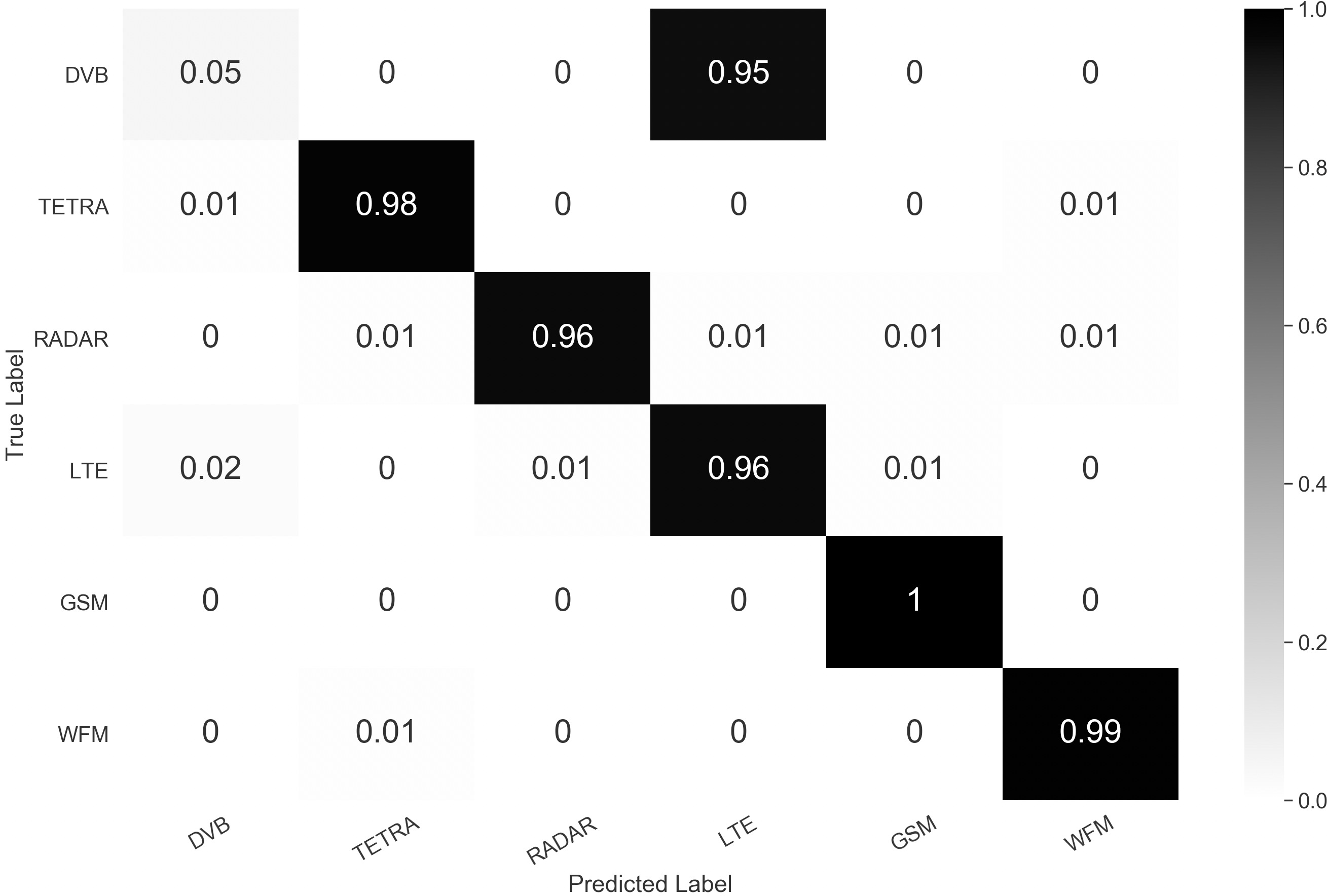
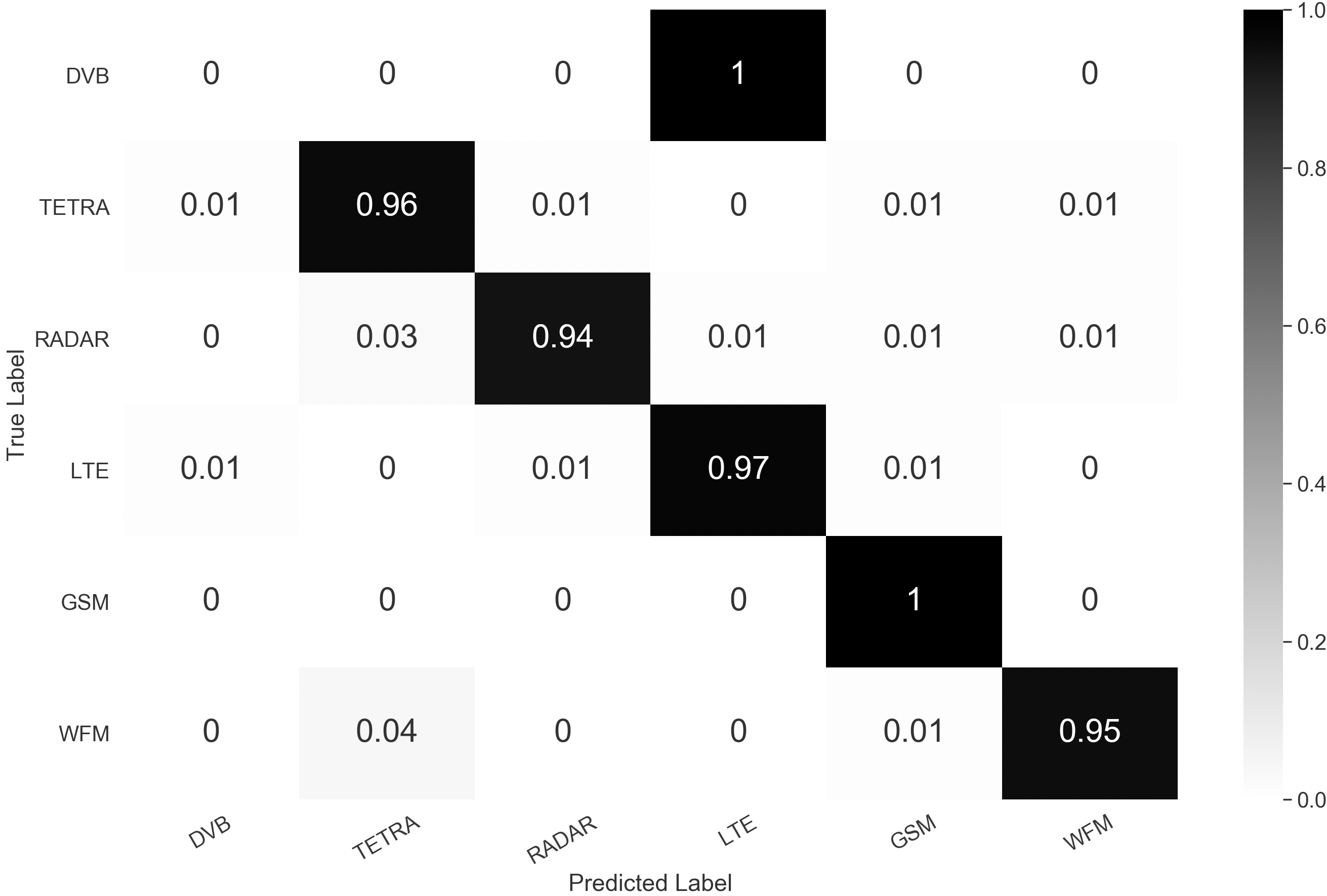
Figure 13: Confusion matrices of the proposed model (top) and LSTM (bottom) for technology classification on Electrosense data.

Figure 13 shows the confusion matrices of our proposed model and LSTM for technology classification on Electrosense data. The proposed model performs slightly better than LSTM. It is noticeable that distinguishing DVB from LTE based on PSD is difficult since the power spectra of DVB and LTE is highly similar and both of them are based on OFDM [12].

Next, we compare the considered models in terms of the number of trainable parameters, the number of FLOPs, the memory cost and the number of classifications per second on different platforms. As shown in Table VII, the proposed model has significantly fewer trainable parameters and requires much fewer FLOPs and memory space. Table VIII shows that the proposed model is on average approximately $4.3\times$ faster than LSTM on Raspberry Pi 4 in terms of the number of classifications per second. On Raspberry Pi 3, the proposed model is on average approximately $6\times$ faster than LSTM. The mean and standard deviation of the number of classifications per second are calculated over 10 experiments on 1024 signals.

TABLE VII: Number of trainable parameters, number of FLOPs and memory cost of the considered models on Electrosense data.

Model	# Parameters	# FLOPs	Memory
DAE	14572	279455	237KB
LSTM	199563	7696283	2.31MB

TABLE VIII: Number of classifications per second on different platforms for Electrosense data.

Platform		DAE	LSTM
GTX 1080Ti	Mean	685.08	613.30
	Std	13.88	10.85
Intel i7-8700K	Mean	77.72	64.08
	Std	1.69	0.76
Raspberry Pi 4	Mean	12.79	2.92
	Std	0.04	0.02
Raspberry Pi 3	Mean	6.45	1.27
	Std	0.06	0.01

IV Conclusions

In this paper, we introduce a denoising auto-encoder to the problem of inferring the modulation and technology type of a received radio signal. In particular, an LSTM auto-encoder is trained to learn stable and robust features from the noise corrupted received signals, reconstruct the original received signals and infer the modulation or technology type, simultaneously. Empirical studies show that the proposed framework generally outperforms top-1 classification accuracy of the competing methods while requiring significantly smaller computation resources. In particular, the proposed framework employs a compact architecture that it can be implemented on affordable computational devices, enabling real-time classification of the received signals at required levels of accuracy.

References

- [1] O. A. Dobre, A. Abdi, Y. Bar-Ness, and W. Su, “Survey of automatic modulation classification techniques: classical approaches and new trends,” IET Communications, vol. 1, no. 2, pp. 137–156, 2007.
- [2] W. A. Gardner, “Signal interception: a unifying theoretical framework for feature detection,” IEEE Transactions on Communications, vol. 36, no. 8, pp. 897–906, 1988.
- [3] W. A. Gardner and C. M. Spooner, “Signal interception: performance advantages of cyclic-feature detectors,” IEEE Transactions on Communications, vol. 40, no. 1, pp. 149–159, 1992.
- [4] W. Gardner, “Spectral correlation of modulated signals: Part i - analog modulation,” IEEE Transactions on Communications, vol. 35, no. 6, pp. 584–594, 1987.
- [5] W. Gardner, W. Brown, and Chih-Kang Chen, “Spectral correlation of modulated signals: Part ii - digital modulation,” IEEE Transactions on Communications, vol. 35, no. 6, pp. 595–601, 1987.
- [6] Z. Yu, “Automatic modulation classification of communication signals,” Ph.D. dissertation, Department of Electrical and Computer Engineering, New Jersey Institute of Technology, 2006.
- [7] A. Fehske, J. Gaeddert, and J. H. Reed, “A new approach to signal classification using spectral correlation and neural networks,” First IEEE International Symposium on New Frontiers in Dynamic Spectrum Access Networks, 2005. DySPAN 2005., no. 144-150, 2005.
- [8] T. J. O’Shea, J. Corgan, and T. C. Clancy, “Convolutional radio modulation recognition networks,” Engineering Applications of Neural Networks, pp. 213–226, 2016.
- [9] N. E. West and T. O’Shea, “Deep architectures for modulation recognition,” 2017 IEEE International Symposium on Dynamic Spectrum Access Networks (DySPAN), pp. 1–6, 2017.
- [10] S. Hochreiter and J. Schmidhuber, “Long short-term memory,” Neural computation, vol. 9, pp. 1735–80, 12 1997.
- [11] F. A. Gers, J. Schmidhuber, and F. Cummins, “Learning to forget: continual prediction with lstm,” 1999 Ninth International Conference on Artificial Neural Networks ICANN 99. (Conf. Publ. No. 470), vol. 2, pp. 850–855, 1999.
- [12] S. Rajendran, W. Meert, D. Giustiniano, V. Lenders, and S. Pollin, “Deep learning models for wireless signal classification with distributed low-cost spectrum sensors,” IEEE Transactions on Cognitive Communications and Networking, vol. 4, no. 3, pp. 433–445, 2018.
- [13] T. J. O’Shea, T. Roy, and T. C. Clancy, “Over-the-air deep learning based radio signal classification,” IEEE Journal of Selected Topics in Signal Processing, vol. 12, no. 1, pp. 168–179, Feb 2018.
- [14] K. Simonyan and A. Zisserman, “Very deep convolutional networks for large-scale image recognition,” arXiv e-prints, p. arXiv:1409.1556, 2014.
- [15] K. He, X. Zhang, S. Ren, and J. Sun, “Deep residual learning for image recognition,” 2016 IEEE Conference on Computer Vision and Pattern Recognition (CVPR), pp. 770–778, 2016.
- [16] S. Rajendran, R. Calvo-Palomino, M. Fuchs, B. Van den Bergh, H. Cordobes, D. Giustiniano, S. Pollin, and V. Lenders, “Electrosense: Open and big spectrum data,” IEEE Communications Magazin, vol. 56, no. 1, pp. 210–217, 2018.
- [17] T. Xu and I. Darwazeh, “Deep learning for over-the-air non-orthogonal signal classification,” arXiv:1911.06174, 2019.
- [18] I. Goodfellow, Y. Bengio, and A. Courville, Deep Learning. MIT Press, 2016.
- [19] P. Vincent, H. Larochelle, Y. Bengio, and P.-A. Manzagol, “Extracting and composing robust features with denoising autoencoders,” Proceedings of the 25th International Conference on Machine Learning, pp. 1096–1103, 2008.
- [20] M.-Y. Chen, T.-C. Huang, V. Shu, C.-C. Chen, T.-C. Hsieh, and N. Yen, “Learning the chinese sentence representation with lstm autoencoder,” Proceedings of WWW ’18: The Web Conference, 2018.
- [21] Z. Ke and H. Vikalo, “A graph auto-encoder for haplotype assembly and viral quasispecies reconstruction,” Proceedings of The Thirty-Fourth AAAI Conference on Artificial Intelligence, pp. 719–726, 2020.
- [22] D. Kingma and J. Ba, “Adam: A method for stochastic optimization,” International Conference on Learning Representations, 12 2014.
- [23] T. O’Shea and N. West, “Radio machine learning dataset generation with gnu radio,” Proceedings of the GNU Radio Conference, vol. 1, no. 1, 2016.
- [24] T. J. O’Shea, J. Corgan, and T. C. Clancy, “Unsupervised representation learning of structured radio communication signals,” 2016 First International Workshop on Sensing, Processing and Learning for Intelligent Machines (SPLINE), pp. 1–5, 2016.