Abstract

Many Polyakov loop models can be written in a dual formulation which is free of sign problem even when a non-vanishing baryon chemical potential is introduced in the action. Here, results of numerical simulations of a dual representation of one such effective Polyakov loop model at finite baryon density are presented. We compute various local observables such as energy density, baryon density, quark condensate and describe in details the phase diagram of the model. The regions of the first order phase transition and the crossover, as well as the line of the second order phase transition, are established. We also compute several correlation functions of the Polyakov loops.

  e-mail addresses: ^†oleg@bitp.kiev.ua,   ^∗Volodymyr.Chelnokov@lnf.infn.it,
^‡emanuelemendicelli@hotmail.it,   ^¶alessandro.papa@fis.unical.it

1 Introduction

The properties of strongly interacting matter at finite temperatures and densities remain in the focus of intensive theoretical and numerical studies (see Ref. [1] for a recent review). The full understanding of these properties is still far from satisfactory, especially at finite baryon chemical potential, due to the famous sign problem. Many approaches to solve this problem, partially or completely, have been designed during the last decades and a certain progress has been achieved within such methods as Taylor expansion and reweighting at small baryon chemical potential, simulations at imaginary potential, complex Langevin simulations and some others (see, e.g., the reviews [2, 3, 4]).

One of the approaches attempting to fully solve the sign problem relies on rewriting the original partition function and important observables in terms of different, usually integer valued, degrees of freedom such that the resulting Boltzmann weight is positive definite. Conventionally, all such formulations are referred to as dual formulations, though sometimes a different name can be used (e.g., flux line representation) [5]. There are several routes to construct such dual theory for non-Abelian lattice models with fermions [7, 6, 8]. While a dual formulation with a positive Boltzmann weight has not yet been constructed for full QCD, positive formulations (or formulations where sign problem appears to be very soft) are already known for few important cases. One such case refers to the strong coupling limit of QCD, where the $SU(N)$ lattice gauge theory can be mapped onto a monomer-dimer and closed baryon loop model [9] (for a recent development of this direction, see Ref. [10] and references therein). Another important case is represented by many effective Polyakov loop models which can be derived from the full lattice QCD in certain limits. A dual representation with positive Boltzmann weight is known for some $SU(N)$ [11, 12, 13] and $U(N)$ Polyakov loop models [6] (for recent advances, see Ref.[14]). Two of these versions have been studied numerically in [12, 13, 15]. The emphasis in these simulations was put on establishing the phase diagram of the model in the presence of the baryon chemical potential and on computing local observables which can be obtained by differentiating the dual partition function with respect to some of the parameters entering the action of the theory.

Important class of observables not yet computed in dual formulations are the correlations of the Polyakov loops. These correlations can be related to screening (electric and magnetic) masses at finite temperatures. Understanding the properties of such masses would lead to an essential progress in our comprehension of the high temperature QCD phase as a whole. While correlations and related masses have been subject of numerous and intensive calculations at zero chemical potential (see [16] and references therein), it seems to be an extremely difficult problem to compute these masses for the real baryon chemical potential with available simulation methods. So far correlations and screening masses have been computed only at imaginary chemical potential in [17]. A closely related and intriguing problem is the appearance of a hypothetical oscillating phase at finite density [18, 19, 20]. Such a phase is ultimately connected to the complex spectrum of the theory and requires computations of long-distance correlations with real baryon chemical potential.

Here and in a forthcoming paper we study a somewhat different, but equivalent dual form of the effective Polyakov loop model presented in [14]. This form of the dual representation has been already used by us in [21] for the computation of correlation functions related to the three-quark potential. We believe it is well suited to address the problem of screening masses at finite densities, at least in the framework of the available positive dual formulations. In the present paper we describe the Polyakov loop model we work with, its dual representation and several observables. We compute also some local observables and reveal the phase structure of the model. We shall also present preliminary results for the Polyakov loop correlations. In a companion paper we will give a detailed study of screening masses, based on the computation of correlation functions and of the second moment correlation length at finite density. This will also allow us to draw some conclusions about the existence of an oscillating phase in the model.

We work on a $3$-dimensional hypercubic lattice $\Lambda=L^{3}$, with $L$ the linear extension and a unit lattice spacing. The sites of the lattice are denoted by $\vec{x}\equiv x=(x_{1},x_{2},x_{3})$, $x_{i}\in[0,L-1]$, while $l=(\vec{x},\nu)$ is the lattice link in the direction $\nu$; $e_{\nu}$ is the unit vector in the direction $\nu$ and $N_{t}$ is the lattice size in the temporal direction. Periodic boundary conditions are imposed in all directions. Let $G$ be the $SU(N)$ group and $U(x)$ an element of $G$, then $dU$ denotes the (reduced) Haar measure on $G$ and ${\rm Tr}U$ the fundamental character of $G$.

In this paper we shall study an effective 3-dimensional Polyakov loop model which describes a $(3+1)$-dimensional lattice gauge theory with one flavor of staggered fermions. The general form of the partition function of the model is given by

$$Z_{\Lambda}(\beta,m,\mu;N,N_{f})\equiv Z\ =\ \int\ \prod_{x}\ dU(x)\prod_{x,\nu}\ B_{\rm g}(\beta)\ \prod_{x}\ B_{\rm q}(m,\mu)\ .$$ (1)

Here, $B_{\rm g}(\beta)$ is the gauge part of the Boltzmann weight and $B_{\rm q}(m,\mu)$ is the determinant for static quarks. There are many forms of $B_{\rm g}(\beta)$ and $B_{\rm q}(m,\mu)$ discussed in the literature. In what follows we use the weight that can be obtained on an anisotropic lattice and in the limit of vanishing spatial gauge coupling $\beta_{\rm s}$ after explicit integration over all spatial gauge fields (see, for instance, Refs. [22, 13, 23] and references therein):

$$B_{\rm g}(\beta)\ =\ \exp\left[\beta\ {\rm Re}{\rm Tr}U(x){\rm Tr}U^{\dagger}(x+e_{\nu})\right]\ .$$ (2)

For $SU(N)$ the effective coupling constant $\beta$ is related to the temporal coupling $\beta_{\rm t}$ by $\beta=2D_{\rm F}(\beta_{\rm t})$ with

$$D_{\rm F}(\beta_{\rm t})\ =\ \left(\frac{C_{\rm F}(\beta_{\rm t})}{NC_{0}(\beta_{\rm t})}\right)^{N_{t}}\ ,\ \ \ C_{\rm F}(\beta_{\rm t})\ =\ \sum_{k=-\infty}^{\infty}\ \Bigl{.}{\rm det}I_{\lambda_{i}-i+j+k}(\beta_{\rm t})\Bigr{|}_{1\leq i,j\leq N}\ ,$$ (3)

where $I_{n}(x)$ is the modified Bessel function and $\lambda_{i}$ refers to the fundamental representation of $SU(N)$ and is equal to $\lambda_{i}=\delta_{1i}$. The Boltzmann weight of static staggered fermions can be presented as

$$B_{\rm q}(m,\mu)\ =\ A(m)\ {\rm det}\left[1+h_{+}U(x)\right]\ {\rm det}\left[1+h_{-}U^{\dagger}(x)\right]\ ,$$ (4)

where the determinant is taken over group indices and

$$A(m)=h^{-N}\ ,\ \ \ h_{\pm}=he^{\pm\frac{\mu_{ph}}{T}}\ ,\ \ \ h=e^{-N_{t}\operatorname{arcsinh}m}\approx e^{-\frac{m_{ph}}{T}}\ .$$ (5)

Below we shall use the dimensionless quantities $m=m_{\rm ph}/T$ and $\mu=\mu_{\rm ph}/T$. Then for $SU(3)$ one has $A(m)=e^{3m}$.

The resulting Polyakov loop model we work with takes the form

$$Z\ = \ \int\prod_{x}dU(x)\exp\left[\beta\sum_{x,\nu}\ {\rm{Re}}{\rm{Tr}}U(x){\rm{Tr}}U^{\dagger}(x+e_{\nu})\right]$$ (6)

$$\times \ \prod_{x}\ A(m)\ {\rm det}\left[1+h_{+}U(x)\right]\ {\rm det}\left[1+h_{-}U^{\dagger}(x)\right]\ .$$

In this model the matrices $U(x)$ play the role of Polyakov loops, the only gauge-invariant operators surviving the integration over spatial gauge fields and over quarks. The integration in (6) is performed with respect to the Haar measure on $G$. The pure gauge part of the $SU(N)$ model is invariant under global discrete transformations $U(x)\to ZU(x)$, with $Z\in Z(N)$. This is the global $Z(N)$ symmetry. The quark contribution violates this symmetry explicitly. Another important feature of the Boltzmann weight is that it becomes complex in the presence of a chemical potential, as it follows from (6). Therefore, the model cannot be directly simulated if $\mu$ is non-zero.

In the absence of static quarks the Polyakov loop model exhibits a first order phase transition at the critical point $\beta_{\rm c}\approx 0.274$. The global $Z(N)$ symmetry gets spontaneously broken above $\beta_{\rm c}$. At finite density the model defined in Eq. (6) and its several variations have been studied both numerically via simulation of dual formulations [12, 13, 15] and analytically via mean-field approximation [24, 25, 26] and via linked cluster expansion [27]. Mean-field and Monte Carlo study are in quantitative agreement for the expectation values of energy density and Polyakov loop. This allowed to reveal the phase diagram of the model, at least in some regions of the parameters $\beta$, $h$ and $\mu$. In this paper we confirm the qualitative picture found in previous study and give further details on the behavior of local observables, including the baryon density and the quark condensate. Also, first results for Polyakov loop correlations will be presented.

The paper is organized as follows. In Section 2 we formulate our dual representation of the model valid for all $SU(N)$ groups and in all dimensions. We present also results of an analytical study of the model based on strong coupling expansion and mean-field approximation. The phase diagram of the 3-dimensional $SU(3)$ model is studied numerically in details in Section 3, where we discuss also simulation results for some local observables as the baryon density and the quark condensate. In Section 4 we present preliminary results for the Polyakov loop correlation functions. The summary and outline for future work is done in Section 5.

2 Dual formulation of the Polyakov loop model

In this Section we describe the dual form of the partition function (6). This dual representation will be used in the next Sections for numerical simulations of the model. All details of the derivation can be found in [14]. In the case of one flavor of staggered fermions the partition function (6) can be presented, after an exact integration over Polyakov loops, as

$$Z=\sum_{\{r(l)\}=-\infty}^{\infty}\ \sum_{\{s(l)\}=0}^{\infty}\ \prod_{l}\frac{\left(\frac{\beta}{2}\right)^{|r(l)|+2s(l)}}{(s(l)+|r(l)|)!s(l)!}\ \prod_{x}A(m)R_{N}(n(x),p(x))\ ,$$ (7)

$$n(x)=\sum_{i=1}^{2d}\left(s(l_{i})+\frac{1}{2}|r(l_{i})|\right)+\frac{1}{2}\sum_{\nu=1}^{d}\left(r_{\nu}(x)-r_{\nu}(x-e_{\nu})\right)\ ,$$ (8)

$$p(x)=\sum_{i=1}^{2d}\left(s(l_{i})+\frac{1}{2}|r(l_{i})|\right)-\frac{1}{2}\sum_{\nu=1}^{d}\left(r_{\nu}(x)-r_{\nu}(x-e_{\nu})\right)\ ,$$ (9)

where $l_{i},i=1,...,2d$ are $2d$ links attached to a site $x$ and

$$R_{N}(n,p)=\sum_{q=-\infty}^{\infty}\sum_{k,l=0}^{N}\sum_{\sigma\vdash n+k}\ \delta_{n+k,p+l+qN}\ d(\sigma/1^{k})d(\sigma+q^{N}/1^{l})\ h_{+}^{k}h_{-}^{l}\ .$$ (10)

The sum over $\sigma$ runs over all partitions of $n+k$, and $d\left(\sigma/1^{m}\right)$ is the dimension of a skew representation defined by a corresponding skew Young diagram, $\sigma+q^{N}=(\sigma_{1}+q,\ldots,\sigma_{N}+q)$ (for more details we refer the reader to Ref. [14]). Equation (7) is valid for all $SU(N)$ groups and in any dimension. Clearly, all factors entering the Boltzmann weight of (7) are positive. Hence, this representation is suitable for numerical simulations. The Kronecker delta-function in expression (10) represents the $N$-ality constraint on the admissible configurations of the integer-valued variables $s(l)$ and $r(l)$. This constraint can be exactly resolved only in the pure gauge model when $h_{\pm}=0$. In this case the dual representation (7) has been already tested by us on an example of 2-dimensional $SU(3)$ model, where we studied correlation functions and three-quark potential [21].

In the following Sections we study the dual representation (7) via Monte Carlo simulations for the 3-dimensional $SU(3)$ model. In this case the function $R_{N}(n,p;h_{\pm})$ takes the form

$$R_{3}(n,p)=Q_{3}(n+1,p)\left(h_{+}+h_{-}^{2}+h_{+}h_{-}^{3}+h_{+}^{3}h_{-}^{2}\right)$$

$$+ Q_{3}(n,p)\left(1+h_{+}^{3}+h_{-}^{3}+h_{+}^{3}h_{-}^{3}\right)+Q_{3}(n,p+1)\left(h_{-}+h_{+}^{2}+h_{+}^{3}h_{-}+h_{+}^{2}h_{-}^{3}\right)$$

$$+ Q_{3}(n+1,p+1)\left(h_{+}h_{-}+h_{+}^{2}h_{-}^{2}\right)+Q_{3}(n+2,p)h_{+}h_{-}^{2}+Q_{3}(n,p+2)h_{+}^{2}h_{-}\ .$$

The function $Q_{3}(n,p)$ is the result of the group integration and is given by [28]

$$Q_{N}(n,p)\ =\ \sum_{\lambda\vdash{\rm min}(n,p)}\ d(\lambda)\ d(\lambda+|q|^{N})\ ,$$ (12)

where $d(\lambda)$ is the dimension of the permutation group $S_{r}$ in the representation $\lambda$, $q=(p-n)/N$ (when $q$ is not an integer $Q_{N}(n,p)=0$).

Important is the fact that both local observables and long-distance quantities can be computed with the help of this dual representation. Explicit expressions for the correlation functions of the Polyakov loops will be given in Section 4. Below we list some local observables which we are going to compute here and which can be obtained by taking suitable derivatives of the partition function (7).

• Magnetization and its conjugate

  $$M\ =\ \left\langle\operatorname{Tr}U(x)\right\rangle\ ,\quad M^{*}\ =\ \left\langle\operatorname{Tr}U^{\dagger}(x)\right\rangle\ ,$$ (13)

• Susceptibility

  $$\chi\ =\ L^{2}\left(\left\langle\left(\operatorname{Tr}U(x)\right)^{2}\right\rangle-\left\langle\operatorname{Tr}U(x)\right\rangle^{2}\right)\ ,$$ (14)

• Energy density

  $$E\ =\ \frac{1}{3L^{3}}\;\frac{\partial\ln Z}{\partial\beta}\ =\ \frac{2}{3\beta L^{3}}\;\sum_{l}\langle 2s(l)+|r(l)|\rangle\ ,$$ (15)

• Baryon density

  $$B\ =\ \frac{1}{L^{3}}\;\frac{\partial\ln Z}{\partial\mu}\ =\ \frac{1}{L^{3}}\;\sum_{x}\langle k(x)-l(x)\rangle\ ,$$ (16)

• Quark condensate

  $$Q\ =\ \frac{1}{L^{3}}\;\frac{\partial\ln Z}{\partial m}\ =\ N-\frac{1}{L^{3}}\;\sum_{x}\langle k(x)+l(x)\rangle\ .$$ (17)

In the last two equations $k(x)$ and $l(x)$ are the summation variables from (10).

Before discussing results of numerical simulations we would like to present some results obtained by simple analytical methods. These results can serve as an additional check of numerical data and lead to a better understanding of the whole phase diagram of the model and of the behavior of the different expectation values.

2.1 Strong coupling expansion

The formulation (7) allows a straightforward expansion in powers of $\beta$. The free energy of the 3-dimensional $SU(3)$ model can be written as

$$F=3m+\ln R_{3}(0,0)+\sum_{k=1}^{\infty}\beta^{k}f_{k}\ .$$ (18)

The first three coefficients $f_{k}$ are given by

$$f_{1} =3\,p_{01}\,p_{10}$$

$$f_{2} =\frac{3}{4}\left(p_{11}^{2}+p_{02}\,p_{20}-22\,p_{01}^{2}\,p_{10}^{2}+5\,p_{02}\,p_{10}^{2}+5\,p_{01}^{2}\,p_{20}+10\,p_{10}\,p_{01}\,p_{11}\right)$$

$$f_{3} =\frac{1}{8}\left(1168\,p_{01}^{3}\,p_{10}^{3}-960\,p_{01}^{2}\,p_{10}^{2}\,p_{11}-480\left(p_{01}\,p_{02}\,p_{10}^{3}+p_{01}^{3}\,p_{10}\,p_{20}\right)\right.$$

$$\quad\left.{}+20\left(p_{03}\,p_{10}^{3}+p_{01}^{3}\,p_{30}\right)+150\,p_{11}\left(p_{02}\,p_{10}^{2}+p_{01}^{2}\,p_{20}\right)\right.$$

$$\quad\left.{}+84\,p_{01}\,p_{10}\left(p_{11}^{2}+p_{02}\,p_{20}\right)+60\left(p_{01}\,p_{10}^{2}\,p_{12}+p_{01}^{2}\,p_{10}\,p_{21}\right)\right.$$

$$\quad\left.{}+30\,p_{11}\left(p_{10}\,p_{12}+p_{01}\,p_{21}\right)+15\,p_{20}\left(p_{03}\,p_{10}+p_{01}\,p_{12}\right)\right.$$

$$\quad\left.{}+15\,p_{02}\left(p_{01}\,p_{30}+p_{10}\,p_{21}\right)+p_{03}\,p_{30}+3p_{12}\,p_{21}\right)\ ,$$ (19)

where $p_{kl}=R_{3}(k,l)/R_{3}(0,0)$ and the coefficients $R_{3}$ can be easily calculated from Eqs. (2) and (12), resulting in

$$R_{3}(0,0) =1+h^{2}+h^{4}+h^{6}+2h^{3}\cosh(3\mu)\ ,$$

$$R_{3}(0,1) =h^{2}e^{-2\mu}\left(1+h^{2}\right)+he^{\mu}\left(1+h^{2}+h^{4}\right)\ ,$$

$$R_{3}(1,0) =h^{2}e^{2\mu}\left(1+h^{2}\right)+he^{-\mu}\left(1+h^{2}+h^{4}\right)\ ,$$

$$R_{3}(0,2) =he^{-\mu}\left(1+h^{2}\right)^{2}+h^{2}e^{2\mu}\left(1+h^{2}\right)\ ,$$

$$R_{3}(2,0) =he^{\mu}\left(1+h^{2}\right)^{2}+h^{2}e^{-2\mu}\left(1+h^{2}\right)\ ,$$

$$R_{3}(1,1) =1+2h^{2}+2h^{4}+h^{6}+2h^{3}\cosh(3\mu)\ ,$$

$$R_{3}(0,3) =R(3,0)=\left(1+h^{2}\right)^{3}+2h^{3}\cosh(3\mu)\ ,$$

$$R_{3}(1,2) =2h^{2}e^{-2\mu}\left(1+h^{2}\right)+he^{\mu}\left(2+3h^{2}+2h^{4}\right)\ ,$$

$$R_{3}(2,1) =2h^{2}e^{2\mu}\left(1+h^{2}\right)+he^{-\mu}\left(2+3h^{2}+2h^{4}\right)\ .$$ (20)

All local observables listed above can be obtained from the expansion (18). The strong coupling expansion converges, presumably in the region $\beta\leq\beta_{\rm c}(h,\mu)$, where $\beta_{\rm c}(h,\mu)$ is the phase transition or crossover point. One expects that in this region numerical data agree reasonably well with strong coupling results. For the purposes of this paper it was sufficient to consider only the lowest three orders in the strong coupling series. Higher orders can be calculated using the linked cluster expansion developed in [27] for a similar Polyakov loop model.

2.2 Mean-field solution

Another obvious approach which can be used to get qualitative description of the model (6) is mean-field approximation. Within the mean-field method one obtains an approximate phase diagram of the model. Also, it allows to calculate various local observables, as the free energy density, the baryon density and some others. We use here one of the simplest mean-field schemes, applied to a similar Polyakov loop model in [24, 25, 26]. In this scheme the mean-field approximation reduces to the following replacement:

$$\sum_{x,\nu}\ {\rm{Re}}{\rm{Tr}}U(x){\rm{Tr}}U^{\dagger}(x+e_{\nu})\longrightarrow\frac{2d}{2}\sum_{x}\left(\omega{\rm{Tr}}U(x)+u{\rm{Tr}}U^{\dagger}(x)\right)\ ,$$ (21)

where

$$u=\langle{\rm{Tr}}U(x)\rangle=\frac{1}{d\beta}\ \frac{\partial\ln Z_{\rm mf}(u,\omega)}{\partial\omega}\ ,\ \omega=\langle{\rm{Tr}}U^{\dagger}(x)\rangle=\frac{1}{d\beta}\ \frac{\partial\ln Z_{\rm mf}(u,\omega)}{\partial u}\ .$$ (22)

The partition function gets the form

$$Z\ =\ \left[Z_{\rm mf}(u,\omega)\right]^{L^{d}}\ ,$$ (23)

$$Z_{\rm mf}(u,\omega)\ = \ A(m)\ \int dU\exp\left[d\beta\left(\omega{\rm{Tr}}U+u{\rm{Tr}}U^{\dagger}\right)\right]$$ (24)

$$\times \ {\rm det}\left[1+h_{+}U\right]\ {\rm det}\left[1+h_{-}U^{\dagger}\right]\ .$$

Using the integration methods developed in [28, 14] the mean-field partition function is presented as

$$Z_{\rm mf}(u,\omega)\ =\ \sum_{r,s=0}^{\infty}\ \frac{(d\beta\omega)^{r}}{r!}\ \frac{(d\beta u)^{s}}{s!}\ R_{3}(r,s)\$$ (25)

and explicit form of $R_{3}(r,s)$ reads

$$R_{3}(r,s)=\sum_{i,j=0}^{1}\ C_{ij}\ Q_{3}(r+i,s+j)+C_{20}\ Q_{3}(r+2,s)+C_{02}\ Q_{3}(r,s+2)\ ,$$ (26)

where the coefficients $C_{ij}$ are given by

$$C_{00} = 2\cosh 3m+2\cosh 3\mu\ ,C_{11}=2\cosh m\ ,\ C_{20}=e^{\mu}\ ,\ C_{02}\ =\ e^{-\mu}\ ,$$

$$C_{10} = 2e^{-\mu}\cosh 2m+2e^{2\mu}\cosh m\ ,C_{01}=2e^{\mu}\cosh 2m+2e^{-2\mu}\cosh m\ .$$ (27)

The mean-field equations (22), as well as all local observables, can now be computed numerically and compared with the strong coupling results and numerical data. In the pure gauge case, $h=0$, one finds a first order phase transition at the critical value $\beta_{\rm g}\approx 0.2615$. This value, as well as the magnetization, matches the corresponding results obtained earlier by the mean-field method [24, 25]. Fig. 1 compares our numerical data with the strong coupling expansion and mean-field results for some typical values $h=0.6,\mu=0.5$. More mean-field results and comparison with simulations will be given in the next Section.

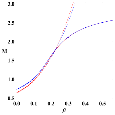
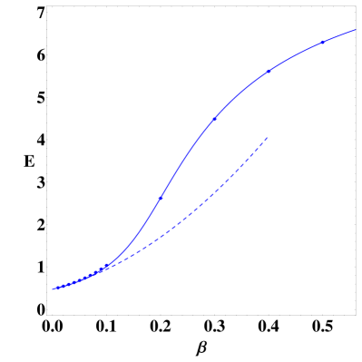
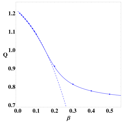
Figure 1: Comparison of the observables obtained from mean-field analysis (solid lines), strong coupling expansion up to third order in $\beta$ (dashed lines) and simulation results (dots) at $h=0.6$, $\mu=0.5$ on a 16³ lattice. Top left: magnetization (blue and red lines denote magnetization and its conjugate, respectively); top right: energy density; bottom left: baryon density; bottom right: quark condensate.

3 Phase diagram of the model

3.1 Lattice setup

To explore the phase structure of the model, we simulate numerically the partition function (7). Important ingredient of such simulations is the way we treat the triality constraint in (10). In the pure gauge theory, $h=0$, this constraint is solved exactly in terms of genuine dual variables and the resulting theory can be simulated with the usual Metropolis update [21]. Instead, at non-zero values of $h$, the function $R_{N}(n,p)$ in (7) is explicitly expanded in series (2). In this formulation every configuration of link variables $s(l)$ and $r(l)$ has non-zero Boltzmann weight, thus allowing us to use again the simple Metropolis update algorithm instead of more complicated worm-like algorithms usually adopted to probe dual model formulations. The values of the function $Q_{3}(n,p)$ are computed beforehand and stored in an array, which is then used in simulations. An extra benefit of the absence of the triality condition is the possibility to calculate a correlation function as the expectation value of a product of one-site observables instead of a product over the path connecting the sources (see Section 4).

Let us mention that our dual formulation allows to simulate all $SU(N)$ models on equal footing: the only difference between different $N$ is encoded in the function $Q_{N}(n,p)$ which, as said above, can be computed prior to simulations. Thus, the present approach can be easily extended to any values of $N$. The investigation of the large-$N$ limit is interesting per sé since it can shed light on the large-$N$ QCD phase diagram at finite density, which could exhibit novel phases, such as quarkyonic matter [29, 30, 31]. Moreover, it can reveal interesting connections between glueball states in $SU(N)$ gauge models for large $N$ and the constituents of dark matter [32].

For simulations above $h=0.01$, we performed $2\cdot 10^{5}$ thermalization updates, and then made measurements every 100 whole lattice updates, collecting a statistic of $10^{5}$ measurements. To estimate statistical error, a jackknife analysis was performed at different blocking over bins with size varying from 10 to $10^{4}$.

When we move to smaller values of $h$, we see that transition probabilities of the one-spin Metropolis update become smaller. To counter this, while keeping the simulation time reasonable, we used the combination of a multihit update with an update skipping procedure: we go through each link variable and attempt $n_{\rm hit}$ Metropolis updates, but before each attempt we calculate the a priori probability that the update is rejected and generate the number $n_{\rm rej}$ of rejects before the first acceptance (from the corresponding geometric distribution); in this way we can skip $n_{\rm rej}$ updates and therefore save on the number of updates left to perform on the current link. Then, if we still need to do some updates, we choose the update for the link using the probabilities calculated in presumption that the update is accepted. Using this technique allows us to vary $n_{\rm hit}$ for different simulation parameters in the range 5 - 2000, while keeping the simulation time constant for a fixed acceptance rate.

Below $h=0.01$ we performed $2\cdot 10^{5}$ thermalization updates, with measurements taken every 50 whole lattice updates, collecting a statistics of $10^{6}$ measurements. The bins size in the jackknife analysis varied from 10 to $10^{5}$.

3.2 Critical behavior

A clear indication of the presence of different phases can be seen from the inspection of the distribution and the scatter plot of the Monte Carlo equilibrium values for the absolute value of the magnetization near a transition value of $\beta$: for some choice of the parameters $h$ and $\mu$, we observe two separate peaks and two separate spots, respectively, which is suggestive of a first order transition; for other choices we see instead just one single peak and a single spot, respectively, as expected for a second order transition or a crossover.

Another indication comes from the behavior of the magnetization and its susceptibility versus $\beta$ near the transition for different values of $(h,\mu)$. Figs. 2-4 show that, when $h$ is kept fixed and $\mu$ is varied from $\mu=0$ to $\mu=2$, the transition softens, the “jump” of the magnetization at the pseudo-critical $\beta$ becoming less steep and the peak of the susceptibility less pronounced, which suggests that different regimes are being explored. According to the finite-size scaling analysis discussed below, the three regimes represented in Figs. 2-4 correspond to first order, second order and crossover, respectively.

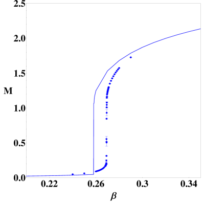
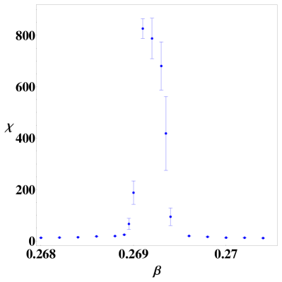
Figure 2: Magnetization (left) and magnetization susceptibility (right) versus $\beta$ at $h=0.01$ and $\mu=0$ on a $16^{3}$ lattice, in the vicinity of a first order phase transition. The solid lines represent the mean-field estimates.

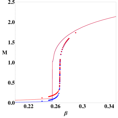
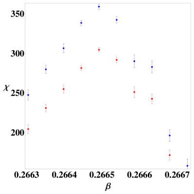
Figure 3: The same as Fig. 2 for $h=0.01$ and $\mu=0.9635$, where a second order phase transition occurs. Lines and points in blue correspond to the magnetization, while those in red correspond to the conjugate magnetization.

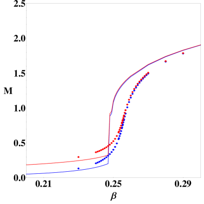
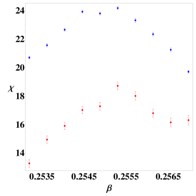
Figure 4: The same as Fig. 3 for $h=0.01$ and $\mu=2$, where a crossover transition occurs.

To characterize in a quantitative way the phase structure of the model in the $(h,\mu)$-plane, we performed a standard finite-size scaling analysis on the peak value of the magnetization susceptibility $\chi$. Although the simulation algorithm does not prevent us from considering arbitrarily large lattice sizes, we limit ourselves to the results presented here, obtained by high-statistic simulations on lattices with linear sizes $L$ = 10 and 16. Larger lattices were also studied for some choices of the couplings to investigate the behavior of the correlation functions. We do not quote those results here to keep a uniform treatment of the whole parameter space. These results will appear in a separate paper. The reason for using relatively small lattice sizes is twofold: on one side, we had to explore a wide region in a three-parameter space and simulating many volumes for each point in the parameter space would have been too expensive; on the other side, drawing a precision phase diagram for this model is beyond the scope of the present work, whose main aim is rather to show the effectiveness of the suggested model. We determined $\chi$ for several $\beta$ values in the transition region and fitted them to a Lorentzian, thus getting the position of the peak, which gives the pseudocritical coupling $\beta_{\rm pc}$, and its height. Comparing the dependence of the peak height on the lattice size $L$ with the scaling law

$$\chi_{L}(\beta_{\rm pc})=AL^{\gamma/\nu}\;,$$ (28)

we estimated the critical-index ratio $\gamma/\nu$ and collected all our determinations, as many as 202, in Table 1. More specifically, for each $(h,\mu)$ pair we extracted $\gamma/\nu$ by the following formula:

$$\dfrac{\gamma}{\nu}=\log_{\frac{16}{10}}\left(\dfrac{\chi_{16}(\beta_{\rm pc})}{\chi_{10}(\beta_{\rm pc})}\right)$$ (29)

and assigned to each determination a statistical error calculated by standard error propagation.

$h$	$\mu$	$\beta_{\rm pc}$	$\gamma/\nu$
0.001	3.0	0.269041(7)	2.83(6)
	3.2	0.267843(5)	2.50(11)
	3.3	0.267156(7)	2.14(5)
	3.35	0.266782(5)	2.06(4)
	3.36	0.266708(1)	1.96(2)
	3.365	0.266669(3)	1.93(2)
	3.375	0.266596(4)	1.88(3)
	3.4	0.266390(4)	1.79(4)
	3.5	0.265563(5)	1.39(4)
	4.0	0.26016(4)	0.07(9)
	5.0	0.2413(2)	0.01(3)
0.002	2.3	0.26904(2)	2.72(10)
	2.4	0.268487(4)	2.48(11)
	2.5	0.267861(5)	2.54(3)
	2.55	0.267526(4)	2.35(3)
	2.6	0.267172(6)	2.24(6)
	2.625	0.266992(5)	2.15(3)
	2.65	0.266809(5)	2.03(4)
	2.8	0.26558(2)	1.49(10)
	3.0	0.26370(3)	0.61(13)
	4.0	0.2485(3)	-0.07(6)
0.003	2	0.26837(2)	2.56(28)
	2.2	0.267102(6)	2.24(4)
	2.25	0.266724(3)	1.97(2)
	2.275	0.266537(5)	1.92(3)
	2.3	0.266339(3)	1.77(2)
	2.5	0.264611(7)	0.99(3)
0.004	1.6	0.268926(9)	2.64(18)
	1.8	0.267786(4)	2.48(3)
	1.88	0.267257(4)	2.22(3)
	1.9	0.267116(6)	2.18(4)
	1.95	0.266758(3)	2.02(3)
	1.96	0.266685(3)	1.98(3)
	1.97	0.266608(4)	1.94(2)
	1.975	0.266574(5)	1.87(3)
	2	0.26637(2)	1.63(22)
	3	0.2542(1)	0.08(6)
0.005	1.5	0.268147(4)	2.58(4)
	1.7	0.266877(4)	2.07(3)
	1.8	0.266137(4)	1.69(3)
	1.85	0.265729(2)	1.50(1)
	2	0.264402(5)	0.98(4)
	2.5	0.25850(5)	0.12(7)
0.007	0.8	0.26947(4)	2.50(46)
	1	0.268710(7)	2.46(14)
	1.2	0.267686(3)	2.52(5)
	1.3	0.267085(4)	2.23(3)
	1.4	0.266403(4)	1.92(5)
	1.5	0.265659(4)	1.53(3)
	2	0.26066(4)	0.21(7)
	3	0.2429(2)	0.16(4)

$h$	$\mu$	$\beta_{\rm pc}$	$\gamma/\nu$
0.008	0	0.2705(2)	3.02(13)
	0.8	0.268774(9)	2.84(5)
	1	0.26787(1)	2.60(11)
	1.2	0.266733(1)	2.06(1)
	1.3	0.266044(2)	1.69(1)
	1.35	0.265672(3)	1.50(2)
	1.5	0.264432(8)	0.99(5)
	2.5	0.25(9)	0.04(4)
0.01	0	0.26916(2)	3.19(60)
	0.01	0.26923(1)	2.87(6)
	0.2	0.26913(2)	2.92(8)
	0.4	0.26872(1)	2.91(10)
	0.7	0.26780(2)	2.50(10)
	0.8	0.26734(2)	2.21(16)
	0.9	0.266844(1)	2.14(6)
	0.95	0.26656(1)	2.04(4)
	0.96	0.266504(5)	2.02(4)
	0.963	0.26648(1)	1.95(3)
	0.96325	0.26649(1)	1.95(3)
	0.9635	0.26649(1)	1.94(4)
	0.964	0.266473(4)	1.95(2)
	0.96425	0.26648(1)	1.97(3)
	0.9645	0.26647(1)	1.98(3)
	0.965	0.26646(1)	1.92(3)
	0.967	0.26646(1)	1.92(3)
	0.97	0.26644(1)	1.92(3)
	0.98	0.26638(1)	1.86(5)
	1	0.26626(1)	1.82(4)
	1. 1	0.26558(1)	1.44(4)
	1.5	0.26204(1)	0.40(5)
	2	0.25543(9)	0.10(5)
0.0125	0	0.26791(1)	2.63(7)
	0.0125	0.26789(1)	2.55(6)
	0.125	0.26785(1)	2.56(4)
	0.2	0.26776(1)	2.57(5)
	0.3	0.26758(1)	2.52(4)
	0.4	0.26735(1)	2.43(4)
	0.5	0.267032(4)	2.32(3)
	0.6	0.266639(4)	2.06(3)
	0.65	0.26641(1)	1.93(4)
	0.7	0.26617(1)	1.83(4)
	0.8	0.26562(1)	1.54(3)
	0.9	0.26499(1)	1.27(7)
	0.95	0.26462(1)	1.08(4)
	0.97	0.26446(1)	0.96(4)
	1	0.26425(1)	0.99(6)
	1.25	0.26205(2)	0.44(8)

$h$	$\mu$	$\beta_{\rm pc}$	$\gamma/\nu$
0.014	0	0.26712(1)	2.39(8)
	0.014	0.267132(4)	2.37(3)
	0.14	0.26706(1)	2.32(3)
	0.16	0.26702(1)	2.32(4)
	0.2	0.26697(1)	2.33(3)
	0.3	0.26678(1)	2.24(4)
	0.4	0.266513(5)	2.11(4)
	0.5	0.266164(5)	1.83(3)
	0.6	0.265716(5)	1.63(2)
	0.8	0.26458(1)	1.04(4)
	0.9	0.26387(1)	0.86(3)
	1	0.26307(1)	0.61(3)
	1.2	0.26117(1)	0.31(4)
	1.4	0.25884(5)	0.12(4)
	2	0.2491(2)	-0.04(4)
0.015	0	0.26660(1)	2.13(6)
	0.015	0.26660(1)	2.19(3)
	0.15	0.26651(1)	2.04(5)
	0.2	0.26644(1)	2.06(4)
	0.3	0.26625(1)	1.94(3)
	0.35	0.26613(1)	1.91(3)
	0.4	0.26596(1)	1.82(3)
	0.45	0.265778(4)	1.71(2)
	0.5	0.26556(1)	1.44(2)
	0.6	0.26510(1)	1.34(3)
0.0155	0	0.26635(1)	1.99(3)
	0.0155	0.26635(1)	2.05(8)
	0.05	0.26635(1)	2.01(3)
	0.07	0.266332(4)	2.02(3)
	0.08	0.266312(5)	1.95(2)
	0.085	0.26632(1)	1.93(4)
	0.09	0.26632(1)	2.04(3)
	0.1	0.26630(1)	1.95(3)
	0.155	0.26625(1)	1.93(4)
	0.3	0.26597(1)	1.86(4)
	0.7	0.26423(1)	1.02(3)
	1	0.26193(2)	0.44(2)
0.0156	0	0.266303(4)	1.94(3)
	0.0156	0.266292(3)	2.01(2)
	0.02	0.266295(4)	1.96(2)
	0.025	0.26629(1)	1.98(4)
	0.0275	0.26631(1)	1.95(2)
	0.03	0.266293(5)	1.94(3)
	0.156	0.26620(1)	1.92(3)
	0.2	0.266121(1)	1.90(4)
	0.4	0.265623(4)	1.61(3)
	0.6	0.26475(1)	1.22(3)
	0.8	0.263497(4)	0.74(3)

$h$	$\mu$	$\beta_{\rm pc}$	$\gamma/\nu$
0.0157	0	0.266252(4)	2.01(3)
	0.0157	0.26625(1)	1.97(3)
	0.02	0.266247(1)	1.97(1)
	0.03	0.26624(1)	1.99(3)
	0.05	0.266235(1)	1.98(3)
	0.07	0.26623(1)	1.92(3)
	0.1	0.26621(1)	1.91(3)
	0.2	0.266072(4)	1.80(2)
0.0158	0	0.266198(3)	1.95(2)
	0.01	0.26620(1)	1.89(3)
	0.0158	0.26619(1)	1.94(4)
	0.02	0.266197(2)	1.91(2)
	0.04	0.266191(4)	1.95(3)
	0.06	0.266180(4)	1.93(2)
	0.08	0.26617(1)	1.90(2)
	0.1	0.266151(4)	1.88(2)
	0.158	0.266085(4)	1.84(2)
0.01585	0	0.26615(1)	1.94(4)
	0.01585	0.266171(4)	1.96(3)
	0.02	0.26617(1)	1.96(4)
	0.025	0.26617(1)	1.88(4)
	0.03	0.26616(1)	1.95(3)
	0.06	0.26615(1)	1.87(4)
	0.1	0.26613(1)	1.92(3)
	0.2	0.26600(1)	1.81(3)
0.0159	0	0.266157(4)	1.90(2)
	0.0159	0.26615(1)	1.93(4)
	0.02	0.266150(5)	1.88(2)
	0.04	0.266152(4)	1.91(2)
	0.06	0.26613(1)	1.93(4)
	0.08	0.266120(4)	1.91(2)
	0.1	0.26611(1)	1.85(3)
	0.159	0.266039(3)	1.87(2)
	0.2	0.26598(1)	1.79(3)
0.016	0	0.26616(1)	1.90(4)
	0.016	0.26609(1)	1.84(4)
	0.16	0.265976(3)	1.87(2)
0.017	0	0.26557(1)	1.69(4)
	0.017	0.26558(1)	1.60(4)
	0.17	0.26545(1)	1.56(3)
0.018	0.018	0.26508(1)	1.42(4)
0.02	0	0.26404(9)	0.87(1)
	0.01	0.26404(1)	1.00(4)
	0.1	0.26398(1)	0.93(4)
	1	0.25865(6)	0.14(3)
0.025	0	0.26156(1)	0.40(2)
0.03	0	0.25913(3)	0.10(2)
0.04	0	0.25466(4)	0.01(2)

Table 1: Summary of the determinations of $\beta_{\rm pc}$ and $\gamma/\nu$ for different values of $h$ and $\mu$.

We can see that, within uncertainties, the values of $\gamma/\nu$ are spread in a range between 3., which implies a first order transition, and zero, which holds for crossover, passing through the second order 3-dimensional Ising value, $\gamma/\nu=1.9638(8)$ [33]. These sparse values of $\gamma/\nu$ are evidently an artifact of the relatively small lattice sizes we could simulate. If we could approach the thermodynamic limit, we would see that values of $\gamma/\nu$ concentrate around the values of 3. (first order), 1.9638(8) (second order in the 3-dimensional Ising class) and 0. (crossover). This is expected since we know that at $\mu=0$ in the pure gauge limit of QCD or for heavy enough quark masses there is a whole region of first order deconfinement transitions in the $m_{\rm u,d}$-$m_{s}$ plane (the famous Columbia plot), delimited by a line of second order critical points in the 3-dimensional Ising class [34]: thereafter, for lower quark masses, the crossover region is met. In the simulations of our effective Polyakov loop model at non-zero density toward the thermodynamic limit we should see the continuation of the line of second order critical points to non-zero values of the chemical potential. For the lattice volumes considered in our study, we are not able to make a clear-cut assignment of each choice of the parameters $h$ and $\mu$ to one of the three transition regions. Using the determination of $\gamma/\nu$, we tried anyhow to make this assignment, extending and modifying the three possible options (first order, second order and crossover) as in Table 2. This makes no sense in the thermodynamic limit, but can be helpful in the present context. In Table 2 we introduced a color code, to help identifying at a glance in which of these regions a given parameter pair $(h,\mu)$ falls.

$\gamma/\nu$	color	phase
$\gamma/\nu\geq$3	green	first order
2.50 $\leq\gamma/\nu<$ 3	light green	more first order than second order
1.98 $<\gamma/\nu<$ 2.50	yellow	more second order than first order
1.94 $\leq\gamma/\nu\leq$ 1.98	red	very close to second order
1.85 $\leq\gamma/\nu<$ 1.94	brown	more second order than crossover
0.3 $\leq\gamma/\nu<$ 1.85	magenta	more crossover than second order
0 $\leq\gamma/\nu<$ 0.3	blue	crossover

Table 2: Color code used to characterize the different phases depending on the value of $\gamma/\nu$.

In Fig. 5(left) each parameter pair $(h,\mu)$ considered in our simulations is represented by a colored dot in the $(h,\mu)$ plane, according to the color code defined in Table 2, allowing us to sketch a tentative phase diagram in the right panel of the same figure. A different visualization of the general phase diagram is presented in Fig. 6, where in a $3d$ plot $\gamma/\nu$ values are reported in correspondence of each $(h,\mu)$ pair.

Figure 5: (Left) Assignment of each parameter pair $(h,\mu)$ to a transition region according to the color code of Table 2. (Right) Estimated phase diagram.

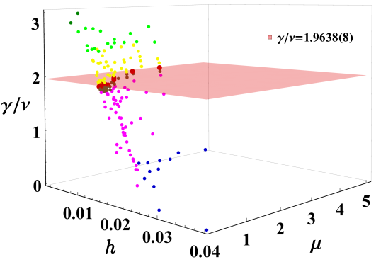
Figure 6: Values of the critical index ratio $\gamma/\nu$ for each considered choice of the pair $(h,\mu)$. The color code is as in Table 2. The plane at $\gamma/\nu=1.9638(8)$ corresponds to the $\gamma/\nu$ value for a second order phase transition in the 3-dimensional Ising class [33] .

Fig. 7 shows the values of $\beta_{\rm pc}$ obtained for each considered pair $(h,\mu)$. It is interesting to note that the variation of $\beta_{pc}$ along the red line (close to the second order phase transition) is much smaller than the variation for all other points. Hence, red points lie approximately in one plane $\beta_{\rm pc}={\rm const}$, while all points associated with other phases lie on a curved surface. This is also seen from Table 3, where we collected the values of $\beta_{\rm pc}$ close to the second order phase transition.

Figure 7: Values of $\beta_{\rm pc}$ for each considered choice of the pair $(h,\mu)$. The color code is as in Table 2. For the sake of readability, red points have been connected by a broken line and the plane $\beta_{\rm pc}=0.266334$ was drawn.

$h$	$\mu$	$\beta_{\rm pc}$	$\gamma/\nu$
0.001	3.36	0.266708(1)	1.96(2)
0.003	2.25	0.266724(3)	1.97(2)
0.01	0.963	0.26648(1)	1.95(3)
0.01	0.96325	0.26649(1)	1.95(3)
0.01	0.9635	0.26649(1)	1.94(3)
0.01	0.964	0.266473(4)	1.95(2)
0.01	0.96425	0.26648(1)	1.97(3)
0.01	0.9645	0.26647(1)	1.98(3)
0.015	0.3	0.26625(1)	1.94(3)
0.0154	0.2	0.26624(1)	1.96(4)
0.0155	0.08	0.266312(5)	1.95(2)
0.0155	0.1	0.26630(1)	1.95(3)
0.0156	0.0	0.266303(4)	1.94(3)
0.0156	0.02	0.266295(4)	1.96(2)
0.0156	0.025	0.26629(1)	1.98(4)
0.0156	0.0275	0.26631(1)	1.95(2)
0.0156	0.03	0.266293(5)	1.94(3)
0.0157	0.0	0.26625(1)	1.97(3)
0.0157	0.02	0.266247(1)	1.97(1)
0.0157	0.05	0.266235(1)	1.98(3)
0.0158	0.0	0.266198(3)	1.95(2)
0.0158	0.04	0.266191(4)	1.95(3)
0.01585	0.0	0.26615(1)	1.94(4)
0.01585	0.01585	0.266171(4)	1.96(3)
0.01585	0.02	0.26617(1)	1.96(3)
0.01585	0.03	0.26616(1)	1.95(3)

Table 3: Values of $\beta_{\rm pc}$ and $\gamma/\nu$ for $h$ and $\mu$ belonging to the region “very close to second order”. These values correspond to the bigger red points in Fig. 7.

We have not performed simulations in the absence of external field. To find the critical value $\beta_{\rm g}$ at $h=0$, i.e. for the pure gauge theory, and at $\mu=0.$, we performed a simple fit of the form $\beta_{\rm c}(h)=\beta_{\rm g}+ah$, as suggested in [13]. We obtained following values $\beta_{g}=0.274991$, $a=-0.5568$. The value of $\beta_{\rm g}$ agrees very well with the value quoted in the literature, $\beta_{\rm g}=0.274$ and reasonably well with the mean-field result $\beta_{\rm g}=0.2615$.

Another important question concerns the shape of the critical line shown in the right panel of Fig. 5 in the heavy-dense limit, $h\to 0$, $\mu\to\infty$. From the data we have, one cannot make unambiguous conclusions about its behavior. Nevertheless, data are well fitted by the function $\mu_{\rm c}=-a\ln h+c-bh^{2}$, with $a=0.932$, $c=-3.1$, $b=2367$. This shows that the line of second order phase transition might persist in the heavy-dense limit of QCD.

3.3 Quark condensate and baryon density

In this subsection we study the behavior of the quark condensate and the baryon density in different phases and compare numerical results with mean-field predictions. In the static approximation for the quark determinant one cannot observe the phenomenon of spontaneous breaking of the chiral symmetry. Indeed, even in the strong coupling region, using Eq. (18), one can easily obtain for the quark condensate $Q=0$ for all $\mu$ in the massless limit $h=1$. The same result in this limit can be obtained within mean-field approach and from numerical simulations which we performed for various values of $\beta$ and $\mu$. Nevertheless, we think it might be instructive to see the behavior of the condensate in the three regimes corresponding to first and second order transitions and to crossover. A more traditional observable to study in the effective Polyakov loop models is the baryon density. In the dual formulation the baryon density $B$ and the quark condensate $Q$ are given by Eqs. (16) and (17), respectively. We have computed the right-hand sides of these equations both numerically and using the mean-field approach, for the same values of $h$ and $\mu$.

The behavior of baryon density and quark condensate as functions of $\beta$ depends strongly on the phase of the system. Left panels of Figs. 8 and 9 show the typical behavior of $Q$ and $B$ for $h=0.01$ and various values of the chemical potential corresponding to different phases of the model. These phases are characterized as before by the values of $\gamma/\nu$ and can be approximately read off from Fig. 6 or, more precisely from the Table 1. One observes a rapid change of both $Q$ and $B$ at the first order phase transition. This rapid change becomes smoother and smoother when parameters are gradually changed toward the second order line and then to the crossover regime. The right panels of the same Figures compare Monte Carlo data with the mean-field predictions in the three regions. One can conclude that mean-field reproduces numerical simulations with good accuracy.

The quark condensate as a function of $\beta$ is shown in Fig. 10(left) for vanishing value of the chemical potential and several values of $h$. The right panel of the same figure demonstrates the approach to the saturation of the baryon density at zero quark mass, $h=1$.

As follows from Fig. 1, the baryon density $B$ is a decreasing function of $\beta$ at sufficiently large $h=0.6$, while Fig. 9 shows that for small $h$ values (large mass) $B$ is an increasing function of $\beta$. This conclusion is supported by all three methods of calculations used in this paper. Therefore, there should exists some value of the quark mass where the density changes its qualitative behavior. We have not tried to estimate this value.

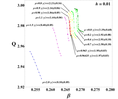
Figure 8: Behavior of the quark condensate versus $\beta$ for fixed $h=0.01$ and for different values of $\mu$ on a 16³ lattice. Left panel: results of simulations in the vicinity of a phase transition. Right panel: comparison of mean-field analysis and numerical results in three different phase regimes. The color code of Table 2 is used here and below to differentiate the phases of the system.

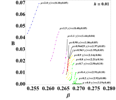
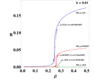
Figure 9: Behavior of the baryon density versus $\beta$ for fixed $h=0.01$ and for different values of $\mu$ on a 16³ lattice. Left panel: results of simulations in the vicinity of a phase transition. Right panel: comparison of mean-field analysis and numerical results in three different phase regimes.

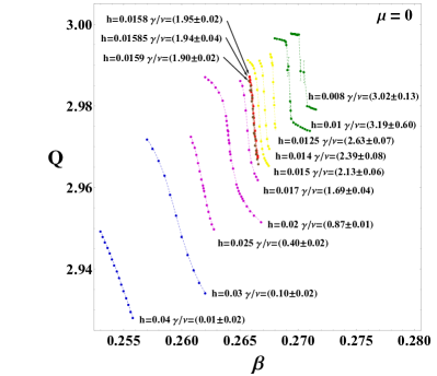
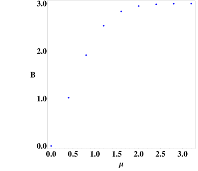
Figure 10: Left panel: behavior of the quark condensate versus $\beta$ for fixed $\mu=0$ and for different values of $h$ on a 16³ lattice. Right panel: baryon density for $h=1$ and $\beta=0.1$ on a 16³ lattice.

4 Large-distance behavior of the correlations

To see the impact of a non-zero chemical potential on the correlation function behavior, we calculated the two-point correlation functions for several values of parameters. We considered six kinds of the correlation functions:

$$\Gamma_{nn}(r) =\left\langle\operatorname{Tr}U(0)\operatorname{Tr}U(r)\right\rangle\ , \Gamma_{rr}(r) =\left\langle\operatorname{Re}\operatorname{Tr}U(0)\operatorname{Re}\operatorname{Tr}U(r)\right\rangle\ ,$$

$$\Gamma_{na}(r) =\left\langle\operatorname{Tr}U(0)\operatorname{Tr}U^{\dagger}(r)\right\rangle\ , \Gamma_{ri}(r) =\left\langle\operatorname{Re}\operatorname{Tr}U(0)\operatorname{Im}\operatorname{Tr}U(r)\right\rangle\ ,$$

$$\Gamma_{aa}(r) =\left\langle\operatorname{Tr}U^{\dagger}(0)\operatorname{Tr}U^{\dagger}(r)\right\rangle\ , \Gamma_{ii}(r) =\left\langle\operatorname{Im}\operatorname{Tr}U(0)\operatorname{Im}\operatorname{Tr}U(r)\right\rangle\ .$$ (30)

In the dual formulation the correlation functions can be written as

$$\Gamma_{nn}(r) =\left\langle\frac{R_{3}(n(0)+1,p(0))}{R_{3}(n(0),p(0))}\frac{R_{3}(n(r)+1,p(r))}{R_{3}(n(r),p(r))}\right\rangle$$

$$\Gamma_{na}(r) =\left\langle\frac{R_{3}(n(0)+1,p(0))}{R_{3}(n(0),p(0))}\frac{R_{3}(n(r),p(r)+1)}{R_{3}(n(r),p(r))}\right\rangle$$

$$\Gamma_{aa}(r) =\left\langle\frac{R_{3}(n(0),p(0)+1)}{R_{3}(n(0),p(0))}\frac{R_{3}(n(r),p(r)+1)}{R_{3}(n(r),p(r))}\right\rangle\ .$$ (31)

These formulas work for $r>0$. For $r=0$ both shifts to the $n$, $p$ variables happen at one point, so only one ratio remains. The correlations $\Gamma_{rr}$, $\Gamma_{ri}$ and $\Gamma_{ii}$ can be obtained as linear combinations of $\Gamma_{nn}$, $\Gamma_{na}$ and $\Gamma_{aa}$.

The expressions (31) become unusable when $h=0$, and can have a bad convergence properties for very small $h$, or very large $\mu$ values. We have checked by comparing the numerical results with the strong coupling expressions for small $\beta$ values, that the results can be relied on for $h>0.005$ and $\mu<3$.

Since we work at non-zero $h$, the average traces can become non-zero, introducing a constant term into the correlation function even in the disordered phase. Due to that, we introduce the subtracted correlation functions, subtracting the corresponding average trace inside the correlations:

$$\Gamma_{nn,\rm sub}(r) =\Gamma_{nn}(r)-\left\langle\operatorname{Tr}U\right\rangle^{2}\ ,$$

$$\Gamma_{na,\rm sub}(r) =\Gamma_{na}(r)-\left\langle\operatorname{Tr}U\right\rangle\left\langle\operatorname{Tr}U^{\dagger}\right\rangle\ ,$$

$$\Gamma_{aa,\rm sub}(r) =\Gamma_{aa}(r)-\left\langle\operatorname{Tr}U^{\dagger}\right\rangle^{2}\ .$$ (32)

For these subtracted correlations we expect an exponential decay,

$$\Gamma(r)=A\frac{\exp(-mr)}{r}\;,$$ (33)

at least in the disordered phase.

Samples of correlation function behavior in different regions of the phase diagram are shown in Figs. 11, 12 and 13. One can see that, indeed, both in disordered and ordered phases, the correlations decay exponentially. While the mass gap, corresponding to the slope of the plots, remains the same for $\Gamma_{nn}$, $\Gamma_{na}$, $\Gamma_{aa}$, $\Gamma_{rr}$ and $\Gamma_{ri}$ correlation functions, it is much larger for the $\Gamma_{ii}$ correlation function. Also the mass gap for the $\Gamma_{ii}$ correlation remains more or less constant, and in particular does not vanish in the vicinity of the phase transition.

The difference in mass gaps can be explained by noting that at $\mu=0$ $\Gamma_{rr}$ and $\Gamma_{ii}$ correspond to the color-magnetic and color-electric sectors having different mass gaps $m_{M}$ and $m_{E}$, $m_{M}<m_{E}$ (see [17]). While at non-zero $\mu$ these two sectors should mix, so all the correlators we study should decay with $m_{M}$, it is possible that in our case the mixing is small causing the real large distance mass gap for the color-electric sector to be visible only on distances larger than the ones for which we have reliable results.

In the ordered phase we observe an increase of the correlation function slope (at the same $\beta$ values) with the increase of $\mu$, implying that the mass gap grows with $\mu$. This means an increase of the screening effects: at finite density non-zero $\mu$ pushes system deeper in the deconfined phase. This is in qualitative accordance with the results of [17] obtained with imaginary $\mu$.

We will address these questions in more detail in a future work, which is under preparation. For now, we can note that at least in the disordered phase also the second moment correlation length for the imaginary-imaginary correlations is substantially different from the one for the real-real correlations.

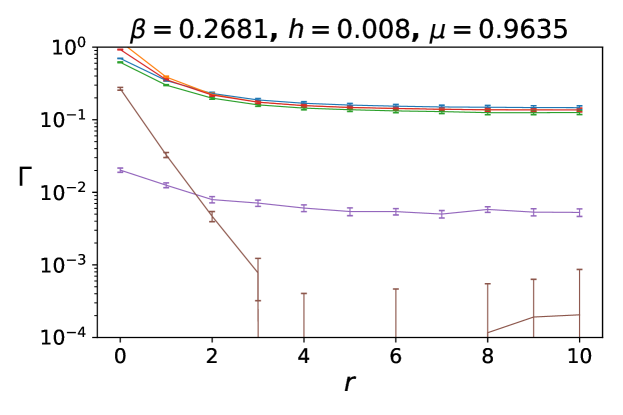
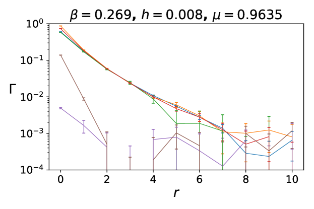
Figure 11: Behavior of the correlation functions on a $20^{3}$ lattice for different values of parameter $\beta$ ($h=0.008$, $\mu=0.9635$). Top: disordered phase. Middle: near the first order phase transition point. Bottom: ordered phase. This legend applies also to the next figures.

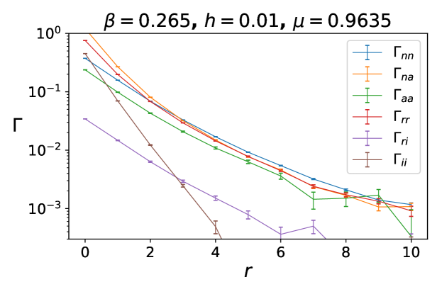
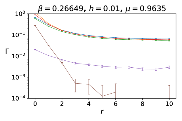
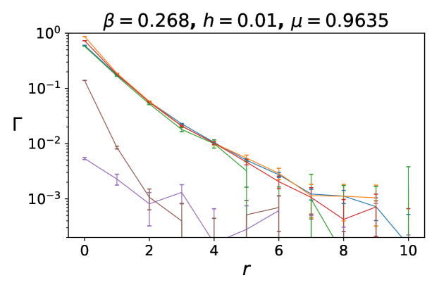
Figure 12: The same as Figure 11 for $h=0.01$, $\mu=0.9635$ (region of the second order phase transition).

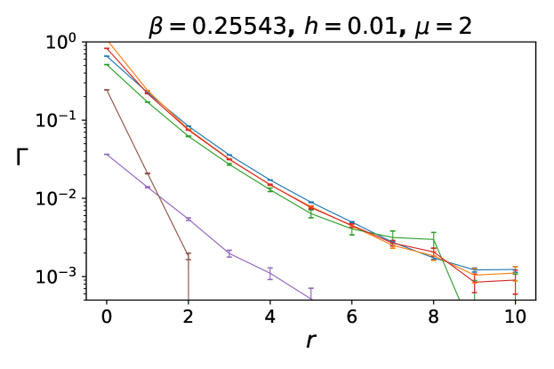
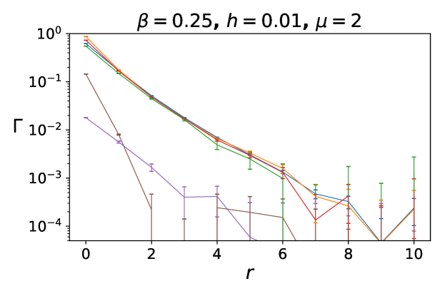
Figure 13: The same as Figure 11 for $h=0.01$, $\mu=2$ (crossover region).

5 Summary

Revealing the phase diagram of QCD at finite temperature and non-zero baryon chemical potential, as well as the nature of strong interacting matter at high temperatures, remains one of the important challenges of high energy physics. In spite of enormous efforts, many aspects of these problems are still far from unambiguous resolution. The several methods developed to solve the sign problem in finite density QCD have their own advantages and drawbacks. Dual formulations of effective Polyakov loop models for heavy-dense QCD, as the one used here, solve the sign problem completely, but are restricted so far to strong coupled regions in the case of non-Abelian gauge theories. Even in this region one can get valuable information about the phase structure of non-Abelian models and behavior of various observables. The study presented here is in the same spirit of Refs. [12, 13, 15], though we have used a different dual formulation of the Polyakov loop model, built in Ref. [14]. To corroborate our findings we have also compared in many cases simulation results with the strong coupling expansion of the dual model and with the mean-field analysis. Let us briefly recapitulate our main results.

• The phase diagram of the model was studied in great details. We have classified three regions in the parameter space of the model $(\beta,h,\mu)$ according to the type of the critical behavior: first or second order phase transition, or crossover. The values of the ratio of critical indices $\gamma/\nu$ is different in different regimes.

• As main observables we computed expectation values of the Polyakov loop and its conjugate, the baryon density and the quark condensate.

• Our dual formulation allows us to compute correlation functions of the Polyakov loops. We have presented some preliminary results for such correlations at non-zero chemical potential.

• It is interesting to note that the mean-field results agree very well with numerical simulations both at zero and non-zero $\mu$. Also, the mean-field results are in good qualitative agreement with a similar analysis in Ref. [24].

The overall qualitative picture of the phase diagram and the behavior of all observables fully agree with the picture described in Refs. [13, 15].

All observables considered in this work have shown sensitivity to the chemical potential. The general trend is that when $\mu$ is increased, they exhibit a less steep variation across transition when the coupling $\beta$ (which corresponds to the temperature in the underlying QCD theory) is increased. Qualitatively, one can say that increasing $\mu$ plays effectively the same role as a reduction of the quark mass.

The most important direction for the future work is a detailed study of the different correlations of the Polyakov loops and the extraction of screening (electric and magnetic) masses at finite chemical potential. Also, an investigation of the oscillating phase and the related complex masses can be accomplished within our dual formulation. All these problems will be addressed in a companion paper which is currently under preparation.

Acknowledgements

Numerical simulations have been performed on the ReCaS Data Center of INFN-Cosenza. O. Borisenko acknowledges support from the National Academy of Sciences of Ukraine in frames of priority project ”Fundamental properties of matter in the relativistic collisions of nuclei and in the early Universe” (No. 0120U100935). The author V. Chelnokov acknowledges support by the Deutsche Forschungsgemeinschaft (DFG, German Research Foundation) through the CRC-TR 211 ’Strong-interaction matter under extreme conditions’ – project number 315477589 – TRR 211. E. Mendicelli was supported in part by a York University Graduate Fellowship Doctoral - International. A. Papa acknowledges support from the Istituto Nazionale di Fisica Nucleare (INFN) through the NPQCD project.

References

- [1] O. Philipsen, PoS LATTICE2019, 273 (2019) [arXiv:1912.04827 [hep-lat]].
- [2] C. Schmidt, PoS LAT2006, 021 (2006) [arXiv:hep-lat/0610116 [hep-lat]].
- [3] P. de Forcrand, PoS LAT2009, 010 (2009) [arXiv:1005.0539 [hep-lat]].
- [4] E. Seiler, EPJ Web Conf. 175, 01019 (2018) [arXiv:1708.08254 [hep-lat]].
- [5] C. Gattringer, K. Langfeld, Int. J. Mod. Phys. A 31, no.22, 1643007 (2016) [arXiv:1603.09517 [hep-lat]].
- [6] O. Borisenko, V. Chelnokov, S. Voloshyn, EPJ Web Conf. 175, 11021 (2018) [arXiv:1712.03064 [hep-lat]].
- [7] C. Marchis, C. Gattringer, Phys. Rev. D 97, no.3, 034508 (2018) [arXiv:1712.07546 [hep-lat]].
- [8] G. Gagliardi, W. Unger, Phys. Rev. D 101, no.3, 034509 (2020) [arXiv:1911.08389 [hep-lat]].
- [9] F. Karsch, K.H. Mütter, Nucl.Phys. B 313 (1989) 541.
- [10] M. Klegrewe, W. Unger, Phys. Rev. D 102, no.3, 034505 (2020) [arXiv:2005.10813 [hep-lat]].
- [11] C. Gattringer, Nucl. Phys. B 850, 242-252 (2011) [arXiv:1104.2503 [hep-lat]].
- [12] Y. D. Mercado, C. Gattringer, Nucl. Phys. B 862, 737-750 (2012) [arXiv:1204.6074 [hep-lat]].
- [13] M. Fromm, J. Langelage, S. Lottini, O. Philipsen, JHEP 01, 042 (2012) [arXiv:1111.4953 [hep-lat]].
- [14] O. Borisenko, V. Chelnokov, S. Voloshyn, Phys. Rev. D 102, no.1, 014502 (2020) [arXiv:2005.11073 [hep-lat]].
- [15] Y. Delgado, C. Gattringer, Acta Phys. Polon. Supp. 5, 1033-1038 (2012) [arXiv:1208.1169 [hep-lat]].
- [16] A. Bazavov and J. H. Weber, Prog. Part. Nucl. Phys. 116 (2021) 103823 [arXiv:2010.01873 [hep-lat]].
- [17] M. Andreoli, C. Bonati, M. D’Elia, M. Mesiti, F. Negro, A. Rucci, F. Sanfilippo, Phys. Rev. D 97, no.5, 054515 (2018) [arXiv:1712.09996 [hep-lat]].
- [18] P. N. Meisinger, M. C. Ogilvie, T. D. Wiser, Int. J. Theor. Phys. 50 (2011) 1042 [arXiv:1009.0745 [hep-th]].
- [19] H. Nishimura, M. C. Ogilvie, K. Pangeni, Phys. Rev. D 93, no.9, 094501 (2016) [arXiv:1512.09131 [hep-lat]].
- [20] O. Akerlund, P. de Forcrand, T. Rindlisbacher, JHEP 10, 055 (2016) [arXiv:1602.02925 [hep-lat]].
- [21] O. Borisenko, V. Chelnokov, E. Mendicelli, A. Papa, Nucl. Phys. B 940, 214-238 (2019) [arXiv:1812.05384 [hep-lat]].
- [22] M. Billò, M. Caselle, A. D’Adda, S. Panzeri, Int. J. Mod. Phys. A 12, 1783-1846 (1997) [arXiv:hep-th/9610144 [hep-th]].
- [23] J. Langelage, M. Neuman and O. Philipsen, JHEP 09, 131 (2014) [arXiv:1403.4162 [hep-lat]].
- [24] J. Greensite, K. Splittorff, Phys. Rev. D 86, 074501 (2012) [arXiv:1206.1159 [hep-lat]].
- [25] J. Greensite, Phys. Rev. D 90, no.11, 114507 (2014) [arXiv:1406.4558 [hep-lat]].
- [26] T. Rindlisbacher and P. de Forcrand, JHEP 02, 051 (2016) [arXiv:1509.00087 [hep-lat]].
- [27] J. Kim, A.Q. Pham, O. Philipsen and J. Scheunert, JHEP 10, 051 (2020) [arXiv:2007.04187 [hep-lat]].
- [28] O. Borisenko, S. Voloshin, V. Chelnokov, Rept. Math. Phys. 85, 129-145 (2020) [arXiv:1812.06069 [hep-lat]].
- [29] L. McLerran and R.D. Pisarski, Nucl. Phys. A 796, 83-100 (2007) [arXiv:0706.2191 [hep-ph]].
- [30] T.J. Hollowood and J.C. Myers, JHEP 10, 067 (2012) [arXiv:1207.4605 [hep-th]].
- [31] O. Philipsen and J. Scheunert, JHEP 11, 022 (2019) [arXiv:1908.03136 [hep-lat]].
- [32] W.C. Huang, M. Reichert, F. Sannino and Z.W. Wang, [arXiv:2012.11614 [hep-ph]].
- [33] A. Pelissetto, E. Vicari, Phys. Rept. 368, 549-727 (2002) [arXiv:cond-mat/0012164 [cond-mat]].
- [34] F. Karsch and S. Stickan, Phys. Lett. B 488, 319-325 (2000) [arXiv:hep-lat/0007019 [hep-lat]].