The SAMI Galaxy Survey: A Statistical Approach to an Optimal Classification of Stellar Kinematics in Galaxy Surveys
Abstract
Large galaxy samples from multi-object Integral Field Spectroscopic (IFS) surveys now allow for a statistical analysis of the galaxy population using resolved kinematic measurements. However, the improvement in number statistics comes at a cost, with multi-object IFS survey more severely impacted by the effect of seeing and lower signal-to-noise. We present an analysis of galaxies from the SAMI Galaxy Survey taking into account these effects. We investigate the spread and overlap in the kinematic distributions of the spin parameter proxy as a function of stellar mass and ellipticity . For SAMI data, the distributions of galaxies identified as regular and non-regular rotators with kinemetry show considerable overlap in the - diagram. In contrast, visually classified galaxies (obvious and non-obvious rotators) are better separated in space, with less overlap of both distributions. Then, we use a Bayesian mixture model to analyse the observed - distribution. By allowing the mixture probability to vary as a function of mass, we investigate whether the data are best fit with a single kinematic distribution or with two. Below , a single beta distribution is sufficient to fit the complete distribution, whereas a second beta distribution is required above to account for a population of low- galaxies. While the Bayesian mixture model presents the cleanest separation of the two kinematic populations, we find the unique information provided by visual classification of galaxy kinematic maps should not be disregarded in future studies. Applied to mock-observations from different cosmological simulations, the mixture model also predicts bimodal distributions, albeit with different positions of the peaks. Our analysis validates the conclusions from previous, smaller IFS surveys, but also demonstrates the importance of using selection criteria for identifying different kinematic classes that are dictated by the quality and resolution of the observed or simulated data.
keywords:
cosmology: observations – galaxies: evolution – galaxies: formation – galaxies: kinematics and dynamics – galaxies: stellar content – galaxies: structure1 Introduction
The distribution of ordered to random stellar motions in present-day galaxies provides strong constraints on how galaxies assembled their mass over cosmic time. Historically, the kinematic properties of spiral galaxies were already known even as the extragalactic nature of these galaxies was still being debated (Slipher, 1914; Pease, 1916). In contrast, the kinematic variety and complexity of early-type galaxies was revealed at a much later stage (for reviews see de Zeeuw & Franx, 1991; Cappellari, 2016). One of the major discoveries for early-type galaxies was that with increasing luminosity, elliptical galaxies transition from being predominantly rapid to predominantly slow rotators (Bertola & Capaccioli, 1975; Illingworth, 1977; Davies et al., 1983), and that the flattening of these slowly-rotating ellipticals was due to anisotropy rather than rotation (Binney, 1978; Schechter & Gunn, 1979).
A key remaining question about the kinematic properties of galaxies is whether the distribution of rotation is bimodal with contrasting formation histories or a continuous transition from one type into another. While there are indications for a bimodal distribution between different types of elliptical galaxies or within the early-type population, most of the evidence is circumstantial. The idea of two intrinsically different types of ellipticals originated from the connection between the kinematic properties of ellipticals with boxy and disky isophotes (Carter, 1987; Bender, 1988; Kormendy & Bender, 1996), or with cuspy cores versus inner power-law stellar light profiles (Faber et al., 1997), that are thought to be related to the merger history.
One of the first mentions of a dichotomy in the early-type population, i.e., two physically distinct groups as based on morphological and photometric properties, is by Ferrarese et al. (1994) further supported by Lauer et al. (1995; but see also Carollo et al. 1997). Subsequently, Kormendy & Bender (1996) suggest a dichotomy between disky and boxy ellipticals based on the relation between the isophotal boxiness parameter and (the ratio of the velocity to the velocity dispersion ), however, they mention the possibility that boxy and disky ellipticals form a continuous sequence. In contrast, Ferrarese et al. (2006) present evidence in favour of a continuous distribution in the logarithmic inner slopes of early-type galaxies, instead of a bimodality. Kormendy & Bender (2012) present an extensive list of properties classifying elliptical galaxies into giant ellipticals () versus normal and dwarf true ellipticals (), a continuation of the results from Kormendy & Bender (1996) and Kormendy et al. (2009). Among other properties, giant ellipticals should have cores, rotate slowly, and have boxy-distorted isophotes.
With two-dimensional (2D) kinematic measurements from integral field spectroscopy (IFS, e.g., SAURON Bacon et al., 2001; de Zeeuw et al., 2002), Emsellem et al. (2007) did not find a clear relation between the spin parameter proxy and boxy versus disky early-types, nor between and core versus power-law early-type galaxies. Further results from ATLAS3D survey indicate no clear trend between the boxiness parameter and the fast rotator (FR) and slow rotator (SR) classes (Emsellem et al., 2011). However, while Krajnović et al. (2013) find no evidence for a bimodal distribution of nuclear slopes of ATLAS3D galaxies, the combination of and is found to be a good predictor for the shape of the inner light profile (see also Krajnović et al., 2020).
In parallel, Emsellem et al. (2007) identified two rotational types of early-type galaxies from a visual inspection of the and maps, quantitatively classified as fast and slow rotators having and , respectively. In subsequent surveys, such as ATLAS3D, a combination of the kinemetry method, which quantifies the regularity of the velocity field (Krajnović et al., 2006; Krajnović et al., 2011), and the spin-parameter proxy and ellipticity were used to classify galaxies as fast and slow rotators (Emsellem et al., 2011). One of the main results from the ATLAS3D survey is that the vast majority of early-types (86%) belong to a single family of fast-rotating disk galaxies with ordered rotation and regular velocity fields (Krajnović et al., 2011; Emsellem et al., 2011). Only a small fraction (14%) of early-type galaxies are slow rotators with more complex dynamical and morphological (e.g., triaxial) structures.
While the evidence for at least two kinematic populations of ellipticals and of early-type galaxies has been growing (e.g., Cappellari, 2016; Graham et al., 2018), there has been relatively little discussion on the possibility of a continuous distribution or on the overlap of properties between classes. Given the complexity of how massive (>10.5) galaxies assemble their stellar mass over time (e.g., see Naab et al., 2014), assigning galaxies to specific classes without expecting considerable overlap might be an unprofitable endeavour. In large volume cosmological simulations (e.g., eagle Schaye et al. 2015, Crain et al. 2015; horizon-agn Dubois et al. 2014; illustris Genel et al. 2014, Vogelsberger et al. 2014; illustris-tng Springel et al. 2018, Pillepich et al. 2018; magneticum Dolag et al., in prep, Hirschmann et al. 2014) the properties of fast and slow rotators have been studied in detail, but the fast/slow selection methods almost always follow the observational criteria (Penoyre et al., 2017; Choi et al., 2018; Lagos et al., 2018b; Schulze et al., 2018; Walo-Martín et al., 2020; Pulsoni et al., 2020). Thus, the question arises as to how much insight we will gain from comparisons to cosmological simulations when quantitatively many fundamental galaxy relations are still poorly matched to observations (van de Sande et al., 2019).
With the rise of large multi-object IFS surveys, such as the SAMI Galaxy Survey (Sydney-AAO Multi-object Integral field spectrograph; N ; Croom et al., 2012; Bryant et al., 2015) and the SDSS-IV MaNGA Survey (Sloan Digital Sky Survey Data; Mapping Nearby Galaxies at Apache Point Observatory; N ; Bundy et al., 2015), we are now able to determine the properties of different kinematic populations as a function of stellar mass using a statistical framework that can be similarly applied when studying mock-galaxies extracted from cosmological simulations. However, the observed kinematic measurements of and in SAMI and MaNGA are more severely impacted by atmospheric seeing as well as having larger kinematic uncertainties due to the lower signal-to-noise (S/N) as compared to earlier IFS surveys (e.g., SAURON, de Zeeuw et al. 2002; ATLAS3D Cappellari et al. 2011; CALIFA, Sánchez et al. 2012). Furthermore, these multi-object IFS samples include galaxies of all morphological types and uncertainties in visual morphological classification could introduce additional challenges. Therefore, a new approach is needed in order to separate non-regular or slow-rotator galaxies from the dominant fast or regular rotating population when the S/N and seeing strongly impact the data quality.
Different methods of correcting the measured for seeing now exist (Graham et al., 2018; Harborne et al., 2020a; Chung et al., 2020), although the corrections are less certain for galaxies with irregular velocity fields. It remains to be seen whether the results from statistical samples of recent IFS surveys are significantly impacted by seeing, such that an intrinsically-bimodal galaxy distribution would be observed as unimodal. Thus, we need to reinvestigate and adapt existing fast and slow rotator selection criteria (e.g., Emsellem et al., 2007, 2011; Cappellari, 2016) and investigate the amount of overlap between the different distributions using multi-object IFS data combined with mock-observations from simulations with relatively low spatial resolution.
In this paper, we revisit dynamical galaxy demographics in the era of large IFS samples, where the impact of seeing and data quality is more severe than in previous IFS surveys. We use the SAMI Galaxy Survey, which contains 3000 galaxies across a large range in galaxy stellar mass, morphology, seeing conditions, and data quality. It provides an ideal test set to investigate the challenges set out above. The main goals of this paper are 1) to determine the impact of different seeing correction methods on the kinematic populations, 2) to investigate the scatter or overlap in the fast and slow rotator distributions, 3) to provide updated methods and selection criteria for separating galaxies that belong to different kinematic families in both observations and simulations, and 4) to consolidate results from different IFS surveys over a range of sample sizes and data quality.
Given the details required to perform a rigorous statistical investigation to achieve our goals, the paper contains several long sections where we analyse and compare previous methods. These sections are independent and can be skipped without losing the main narrative. We present the data from the observations in Section 2. The core analysis of observational data is presented in 3, and for large cosmological simulations in Section 4. Readers solely interested in our new classification method can choose to skip Sections 3.1-3.3 and 4. Section 5 gives our perspective on previous claims of a bimodality (5.1-5.5) as well as a discussion on the implications of this work (5.6-5.7). A summary and conclusion is given in Section 6. Throughout the paper we assume a CDM cosmology with =0.3, , and km s-1 Mpc-1.
2 Data
2.1 SAMI Galaxy Survey
SAMI is a multi-object IFS mounted at the prime focus of the 3.9m Anglo-Australian Telescope (AAT), with 13 hexabundles (Bland-Hawthorn et al., 2011; Bryant et al., 2011; Bryant & Bland-Hawthorn, 2012; Bryant et al., 2014) deployable over a 1 degree diameter field of view. Each hexabundle consists of 61 individual 16 fibres, and covers a diameter region on the sky. The 793 object fibres and 26 individual sky fibres are fed into the AAOmega spectrograph (Saunders et al., 2004; Smith et al., 2004; Sharp et al., 2006), with a blue (3750-5750Å) and red (6300-7400Å) arm. With the 580V and 1000R grating, the spectral resolution is R at 4800Å, and R at 6850Å (Scott et al., 2018), respectively. In order to cover gaps between fibres and to create data cubes with 05 spaxel size, all observations are carried out using a six- to seven-position dither pattern (Sharp et al., 2015; Allen et al., 2015).
The SAMI Galaxy Survey (Croom et al., 2012; Bryant et al., 2015) contains galaxies between redshift with a broad range in galaxy stellar mass (MM⊙) and galaxy environment (field, groups, and clusters). Galaxies were selected from the Galaxy and Mass Assembly (GAMA; Driver et al., 2011) campaign in the GAMA G09, G12 and G15 regions, in combination with eight high-density cluster regions sampled within radius (Owers et al., 2017). We use 3072 unique galaxies from internal data release v0.12. Reduced data-cubes and stellar kinematic data products for 1559 galaxies in the GAMA fields are available as part of the first, second, and third SAMI Galaxy Survey data releases (Green et al., 2018; Scott et al., 2018; Croom et al., 2021).
2.1.1 Ancillary Data
For galaxies in the GAMA fields, aperture matched colours were measured from reprocessed SDSS Data Release Seven (York et al., 2000; Kelvin et al., 2012), by the GAMA survey (Hill et al., 2011; Liske et al., 2015). For the cluster environment, photometry from the SDSS (York et al., 2000) and VLT Survey Telescope (VST) ATLAS imaging data are used (Shanks et al., 2013; Owers et al., 2017). Stellar masses are derived from the rest-frame -band absolute magnitude and colour, by employing the colour-mass relation as outlined in Taylor et al. (2011). A Chabrier (2003) stellar initial mass function and exponentially declining star formation histories are assumed in deriving the stellar masses. For more details see Bryant et al. (2015).
We use the Multi-Gaussian Expansion (MGE; Emsellem et al., 1994; Cappellari, 2002) technique, and the code from Scott et al. (2013) to derive structural parameters of galaxies from the imaging data from the GAMA-SDSS (Driver et al., 2011), SDSS (York et al., 2000), and VST (Shanks et al., 2013; Owers et al., 2017). Those parameters are the effective radius (the half-light radius of the semi-major axis; ), the ellipticity of the galaxy within one effective radius (), and position angles. For more details, we refer to D’Eugenio et al. (in prep).
Visual morphological classifications are described in detail in Cortese et al. (2016). The classifications are determined from SDSS and VST gri colour images and are based on the Hubble type (Hubble, 1926), following the scheme used by Kelvin et al. (2014). Early- and late-type galaxies are divided according to their shape, the presence of spiral arms and/or signs of star formation. Early-types with disks are then classified as S0s and pure bulges as ellipticals (E). Late-types galaxies with a disk plus bulge component are classified as early-spirals, and galaxies with only a disk component as late-spirals.
2.1.2 Stellar Kinematics
The stellar kinematic measurements for the SAMI Galaxy Survey are described in detail in van de Sande et al. (2017b). A short summary is provided below. We use the penalized pixel fitting code (pPXF; Cappellari & Emsellem, 2004; Cappellari, 2017) assuming a Gaussian line-of-sight velocity distribution (LOSVD). Before combining the blue and red spectra, the red spectra are convolved to match the instrumental resolution in the blue. The combined spectra are rebinned onto a logarithmic wavelength scale with constant velocity spacing (57.9 km s-1). We derive a set of radially-varying optimal templates from the SAMI annular-binned spectra, using the MILES stellar library (Sánchez-Blázquez et al., 2006; Falcón-Barroso et al., 2011). For each individual spaxel, pPXF is given a set of two or three optimal templates from the annular bin in which the spaxel is located as well as the optimal templates from neighbouring annular bins. We estimate the uncertainties on the LOSVD parameters from 150 simulated spectra.
We visually inspect the 3072 SAMI kinematic maps in the GAMA and cluster regions, and 140 galaxies are flagged and excluded due to unreliable kinematic maps caused by nearby objects or mergers that influence the stellar kinematics of the main object. 1025 galaxies are excluded because the radius out to which we can accurately measure the stellar kinematics is less than 20 or <15. We also remove 40 galaxies where the ratio of the point-spread-function to the effective radius of a galaxy is larger than . We adopt the limit of 0.6 because of the relatively large impact of beam-smearing on at these values (see Harborne et al., 2020a). Lastly, for another 35 galaxies no reliable aperture correction out to one could be derived (see Section 3.1). This brings the total sample of galaxies with kinematic measurements to 1832.
The stellar kinematic completeness as compared to the full SAMI Galaxy Survey sample is presented in Fig. 1. The largest fraction of galaxies without kinematic measurements is below stellar mass of . Because the stellar kinematic completeness drops rapidly below 50 percent at low stellar mass (see Fig. 1), we do not use the remaining 67 galaxies below for the core analysis of this paper.
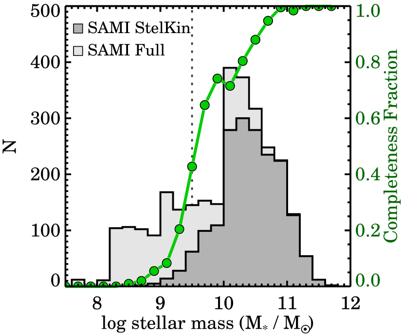
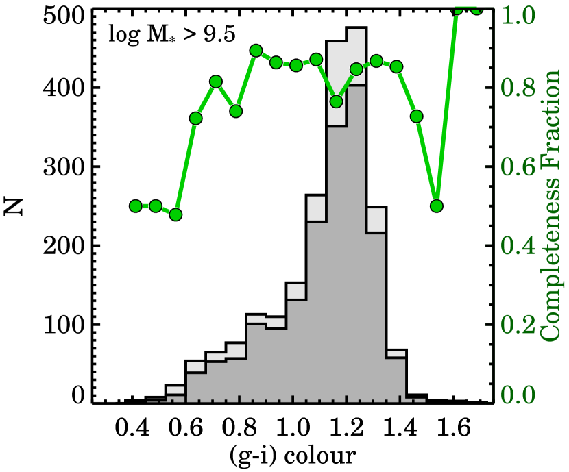
We investigate whether the kinematic sample above this mass limit of is a representative subset of the full SAMI sample by comparing the colour distributions in Fig.2. For the vast majority of the sample ( percent) we find that the colour distribution of the stellar kinematic sample matches that of the full sample, with the exception of the bluest () and some of the reddest () galaxies where the completeness drops below 75 percent. Thus, we conclude that the kinematic sample has no colour bias as compared to the full SAMI sample which was drawn from the volume-limited GAMA survey with high completeness ( percent). The final number of galaxies from the SAMI Galaxy Survey with usable stellar velocity and stellar velocity dispersion maps above a stellar mass of is 1765; we dub this set of galaxies the "SAMI stellar kinematic sample".
3 Kinematic Identifiers in Seeing-Impacted Data
3.1 Fast and Slow Rotators in Seeing Impacted Data
Fast and slow rotator galaxies are commonly selected from a combination of the spin parameter proxy (Emsellem et al., 2007) and the ellipticity . quantifies the ratio of the ordered rotation and the random motions in a stellar system, and is given by:
| (1) |
Here, the subscript refers to the position of a spaxel within the ellipse, the flux of the spaxel, is the stellar velocity in km s-1, the velocity dispersion in km s-1. is the semi-major axis of the ellipse on which spaxel lies, not the circular projected radius to the centre as is used by e.g., Emsellem et al. (2007, 2011). We use the unbinned flux, velocity, and velocity dispersion maps as described in Section 2.1.2. The sum is taken over all spaxels within an ellipse with semi-major axis and ellipticity where the ellipticity is defined from the axis ratio: . We use the input galaxy catalogue’s R.A. and Dec. and WCS information from the cube headers, to determine a galaxy’s centre. The systemic velocity is determined from 9 central spaxels ( box).
We only use spaxels that meet the quality criteria for SAMI Galaxy Survey data as described in van de Sande et al. (2017b): S/N Å-1, FWHM km s-1 where the FWHM is the full-width at half-maximum, km s-1(Q1 from van de Sande et al., 2017b), and km s-1 (Q2 from van de Sande et al., 2017b). In practise, as the uncertainties on and are strongly correlated with S/N, primarily spaxels towards the galaxy outskirts fail to meet these selection criteria. Kinematic maps with spatially discontinuous or measurements (with "holes") are rare, but if the fill factor of good spaxels is less than 85 percent, the galaxy is excluded from the sample. As outlined in van de Sande et al. (2017a), if the fill factor within one effective radius is less than 95 percent, an aperture correction to is applied (279 galaxies, 15.8 percent of the stellar kinematic sample).
Slow rotators are commonly selected using one of the following criteria, i.e., from Emsellem et al. (2007, dotted line in Fig. 3):
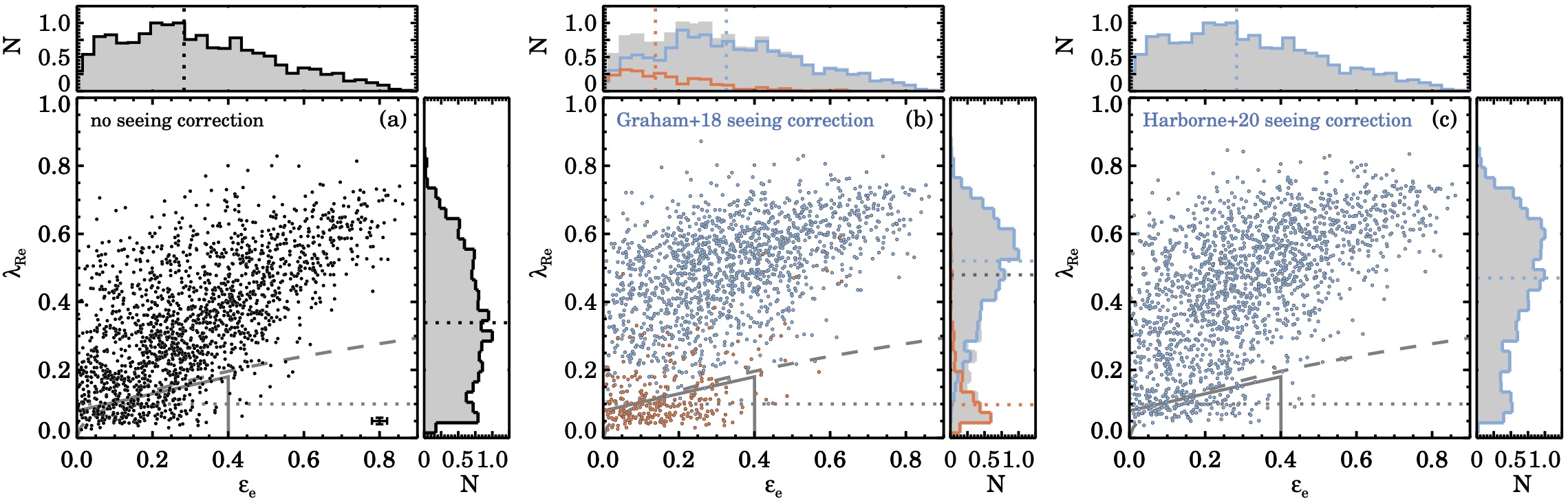
We present the SAMI stellar kinematic sample in Fig. 3(a). The distribution of galaxies in the - space is similar to previous studies (Emsellem et al., 2011; Cappellari, 2016; Graham et al., 2018; Falcón-Barroso et al., 2019). As noted by Falcón-Barroso et al. (2019), in contrast to the CALIFA Survey, our sample does not reach values above . This ceiling is partially caused by the impact of atmospheric seeing (see next paragraph), but also because of the different radius definition used to calculate in Equation 1. A similar effect due to seeing is seen in the MaNGA data as presented by Fraser-McKelvie et al. (2018), but not in Graham et al. (2018); Graham et al. (2019) using the same MaNGA data and definition, who find that reaches values close to the upper limit of 1.0, with and without a seeing correction applied. In the distribution function (Fig. 3a) we see a small peak below , but no clear evidence for two distinct peaks or populations is visible from our seeing-uncorrected data.
Atmospheric seeing impacts the stellar kinematic measurements by spatially smearing the line-of-sight velocity distribution, which results in a flatter observed velocity gradient but increased overall velocity dispersion. Hence, the seeing-impacted values will be lower compared to no-seeing measurements. An analytic correction to account for atmospheric seeing on was presented by Graham et al. (2018). This correction was derived by simulating the effect of seeing on kinematic galaxy models constructed with the Jeans Anisotropic MGE modelling method (Cappellari, 2008), and takes into account the ratio of the seeing to the galaxy effective radius and Sérsic index.
The accuracy of the analytic correction was tested in Harborne et al. (2019). Although the mean correction across a range of morphological types works well, a residual scatter of remains as a function of inclination. However, the correction is applicable only for regular rotators (Graham et al., 2018). The impact of this limitation is demonstrated in Fig. 3(b). Here, we have seeing-corrected for all regular rotating galaxies (blue circles), identified using kinemetry with (see Section 3.2 and van de Sande et al., 2017b), whereas the non-regular rotators are left uncorrected (orange circles). From the distribution shown on the side of Panel (b), a clear bimodal distribution appears111We adopt the definition of bimodality as a distribution with two different modes that appear as distinct peaks in the density distribution., although we argue that this separation is artificial enhanced by the seeing correction.
An alternative seeing correction was presented by Harborne et al. (2020a) that has been derived from a suite of hydrodynamical simulations of galaxies with different bulge-to-total ratios. While the method follows the idea of Graham et al. (2018), this new correction includes an inclination term approximated from the observed ellipticity. The residual scatter in after applying this correction on a test set of galaxies shows smaller residual scatter as compared to Graham et al. (2018), and also works for all galaxy types within the suite of simulations. Yet, true slow rotators, with complex stellar orbital distributions, kinematically distinct cores, and counter rotating disks, are harder to produce in isolated-galaxy simulations. Instead, galaxies from the eagle simulations were used which showed that can be seeing-corrected effectively for this type of galaxy with an accuracy of dex. Furthermore, the absolute impact of the seeing correction on for this galaxy type is small. The Harborne et al. (2020a) seeing-corrected measurements are presented in Fig. 3(c). The low- peak that was visible in Fig. 3(b) distribution is no longer as pronounced, and whilst there may be two populations, by eye it is not clear where and how to divide the two possible distributions.
Including a seeing correction is crucial for recovering an unbiased distribution. As galaxies with smaller angular sizes are more severely impacted by seeing, intrinsic differences in the physical sizes of early- and late-type galaxies combined with a redshift-dependent mass selection, can lead to a morphologically biased distribution. Therefore, in what follows we will use the seeing correction from Harborne et al. (2020a) as the default. The optimised correction formulae for the SAMI Galaxy Survey data are presented in Appendix A.1.
However, with the seeing correction applied to all galaxies, it is unclear whether the Emsellem et al. (2011) or Cappellari (2016) slow rotator selection regions are still valid for our data, or how much overlap there is between the different distributions. As the beam smearing of galaxies with complex inner rotational velocity and dispersion structures behaves differently from regular rotating galaxies, the impact of seeing cannot straightforwardly be predicted with a simple analytic formula; the values for complex non-rotating galaxies might be over-corrected. This could explain why it is harder to detect a bimodal distribution in Fig. 3(c). To solve this problem, we will need to include more information than and alone if we want to determine whether or not we can separate a population of fast and slow rotators in our data.
3.2 Kinemetry: Regular and Non Regular Rotators
3.2.1 Description of the kinemetry method
We first turn to kinemetry for identifying kinematic sub-groups as defined in Krajnović et al. (2011), because the fast and slow rotator selection regions from Emsellem et al. (2011) and Cappellari (2016) were designed to best separate regular and non-regular galaxies. In this section we follow a similar approach. The kinemetry method (Krajnović et al., 2006; Krajnović et al., 2008) provides an estimate of the kinematic asymmetry, under the assumption that the velocity field of a galaxy can be described with a simple cosine law along ellipses: , where is the amplitude of the rotation and is the azimuthal angle. Deviations from this cosine law can then be modelled using Fourier harmonics, where the first order decomposition is equivalent to the rotational velocity and the high-order terms (, ) then describe the kinematic anomalies. The kinematic asymmetry is defined from the amplitudes of the Fourier harmonics (Krajnović et al., 2011). Our method for measuring the kinematic asymmetry on SAMI Galaxy Survey data is described in detail in van de Sande et al. (2017b). The kinemetry method forms the basis of separating galaxies into regular versus non-regular classes. As was already noted in van de Sande et al. (2017b), the distribution of does not show a sharp transition between regular and non-regular rotators. Instead there is a peak in the distribution around with a long tail towards high values (see also Fig. 16a).
Following Emsellem et al. (2011) we use the lower limit to separate regular and non-regular rotators, taking into account that within uncertainties a galaxy that is classed as non-regular rotator can still be a regular rotator. From here on, we simply refer to within an aperture of one effective radius as . The divide between Regular Rotators (RR) and Non-Regular Rotators (NRR) was set to 4 percent in Krajnović et al. (2011) based on the peak and error of the distribution, but to 2 percent in Krajnović et al. (2008). As our data quality is different (median =0.014 for ATLAS3D versus a median =0.029 here), we adjust this limit to =0.07 which corresponds to the 84th percentile of the distribution. Note that in van de Sande et al. (2017b) we also adopted an intermediate class of Quasi-Regular Rotators, but for the clarity of directly comparing to fast and slow rotators, we do not use the QRR terminology here.
3.2.2 Identifying Fast and Slow rotators using kinemetry as a prior
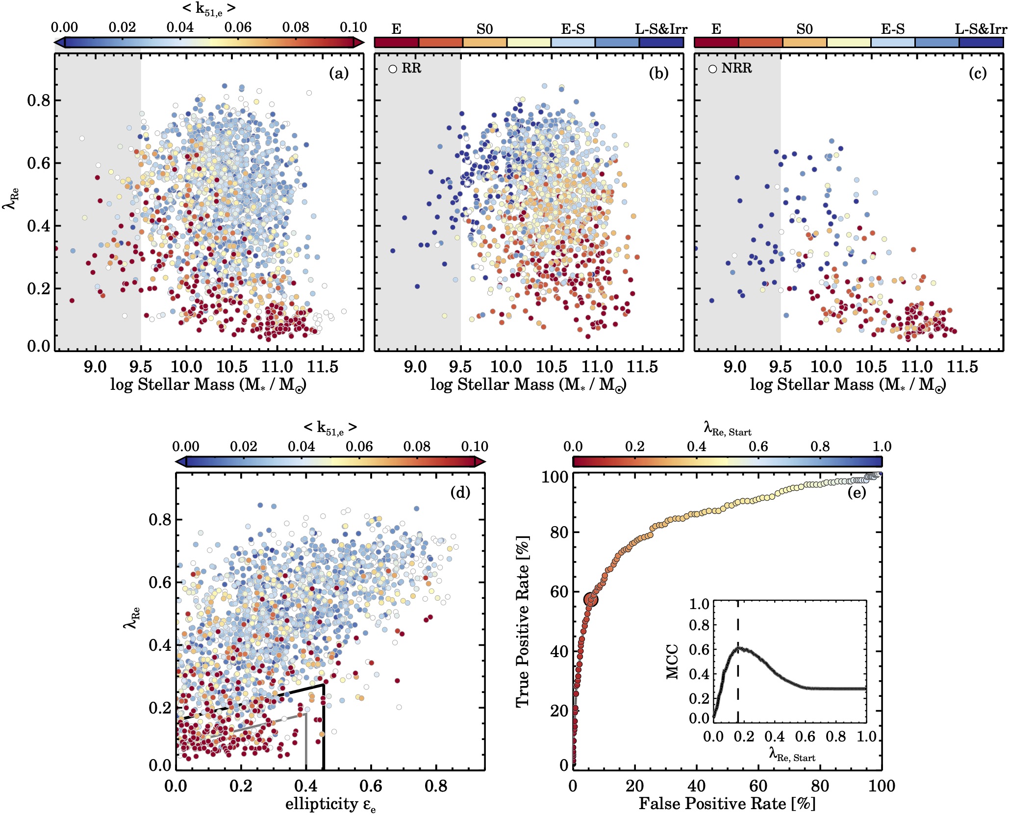
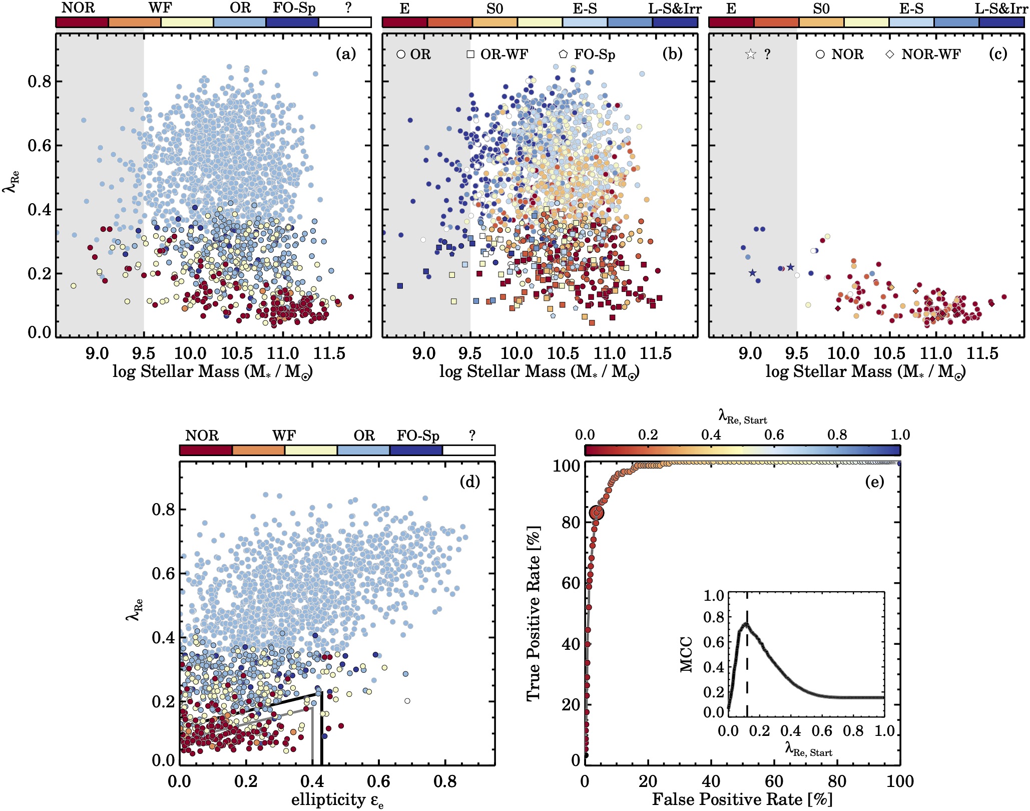
Fig. 4(a) shows the seeing-corrected spin parameter proxy using the method from Harborne et al. (2020a) versus stellar mass . The data are colour coded by the values for the entire sample. There are two clear trends visible. First, at fixed stellar mass, the kinematic asymmetry is higher for low values. Secondly, at fixed the mean kinematic asymmetry becomes higher towards lower stellar mass, likely to be dominated by a relationship in (rotational velocity) versus stellar mass. To clarify these trends, we show the RRs and NRR separately in Fig. 4(b) and 4(c) now colour-coded by visual morphology. As expected, for galaxies with high stellar masses (), NRRs have the lowest values of . However, towards lower stellar mass NRRs demonstrate a large range in , even with our strict definition of non-regularity (). We note that the relatively high-spin NRRs () roughly fall into two categories: galaxies with late-type spiral morphology and inclination with kinematic features in the velocity maps caused by spiral arms or bars, and galaxies with edge-on morphology and low spatial coverage.
The increased scatter in towards low stellar masses is caused by a combination of lower and a decrease in the overall rotational velocities () of these galaxies. Because is normalised by , slower-rotating galaxies that follow a perfect cosine rotation will have higher even if uncertainties on measurements are the same. As galaxies have lower angular momentum towards low stellar mass, higher values of are expected. Similarly, as galaxies are inclined from edge-on towards face-on, will become lower, increasing the typical . Galaxies towards low stellar mass and face-on disks with low surface brightness also have lower typical S/N values, causing higher uncertainties and, therefore, higher . Thus the higher scatter in below is caused by a combination of late-type morphology and observational effects.
The larger scatter between and leads to considerable overlap between the RR and NRR populations in the - diagram. By using a single cut-off value to separate regular and non-regular rotators we will not only cause a bias with stellar mass, but also create a large number of false positives and false negatives, if we assume that is the perfect classifier.
The versus ellipticity diagram, as presented in Fig. 4(d), is now commonly used to separate fast and slow rotators, where the empirical separation between fast and slow rotators is motivated by the location of the regular and non-regular rotators. However, from Fig. 4(d) it is immediately clear that the most-current selection criterion from Cappellari (2016) (grey lines) and the previous selection criteria (Emsellem et al., 2007, 2011, not shown), are unsuccessful in separating RRs and NRRs within our seeing-corrected SAMI sample.
In order to quantify the "success" of the SR selection region for separating RRs and NRRs, we will treat "non-regularity" as a condition that a galaxy can have, while using the - diagram as the diagnostic to identify this condition. By adopting this classification, we can calculate statistical measures of performance of this binary test, such as the sensitivity and specificity. To do so, we first construct a confusion matrix (Table 1) where we determine the True Positives (TP), True Negatives (TN), False Positives (FP), and False Negatives (FN). A true positive is where a galaxy has the condition of NRR and is also classified (i.e., tested positive) as an SR, whereas a True Negative is an RR that has been classified as an FR.
| NRR | RR | |
|---|---|---|
| SR | True Positive | False Positive |
| FR | False Negative | True Negative |
There are several statistical measures that quantify the relevance of our statistical test. Here, we will use an "Receiver Operating Characteristic Curve" analysis to quantify how well our test performs (see for example Fawcett, 2006). Specifically, we will use the sensitivity or true positive rate (), the fall-out or False Positive Rate (), the Positive Prediction Value (), and Matthews correlation coefficient (; Matthews, 1975):
| (2) |
| (3) |
| (4) |
| (5) |
Instead of calculating a single set of numbers for the Cappellari (2016) FR/SR selection, it will be more insightful to try a variety of selection criteria to determine the optimal selection region. We first explored the full range of selection boxes with different starting and end positions (i.e., with different slopes) in both and and but the retrieved optimal selection function did not have significantly improved MCC values as compared to the adopted selection function below (there was one exception that we will highlight in Section 3.4). Instead we choose a varying selection region similar to Cappellari (2016) as this was well-motivated for higher-S/N and higher-spatial resolution data (e.g., see Appendix B.1):
| (6) |
We define the optimal selection when the MCC reaches its highest value, which is a trade off between the number of true and false positives and negatives. We note that there are several other optimisation parameters, such as the "Youden’s J statistic", the Accuracy, or the F1 score, but they all returned similar results as compared to the MCC.
We show the True Positive Rate versus the False Positive Rate, also known as the "Receiver Operating Characteristic Curve" (ROC-curve), in Fig. 4(e), with an additional inset panel that shows the MCC as a function of . A completely random test would result in data residing on the one-to-one line. We test 200 different selection regions, with ranging from 0-1. With increasing values of we find an increase in the TPR but also in the FPR. According to the MCC parameter, the optimal selection region has shown as the black line in Fig. 4(d). This value is significantly higher than the from Cappellari (2016). More importantly, the optimal selection region only has a TPR of 57.4 percent with a FPR of 5.7 percent, and a Positive Prediction Value of 65.8 percent.
Thus, we conclude that using the - diagram to separate regular and non-regular rotators is only moderately successful when presented with seeing-dominated data. We emphasise that the kinemetry method was designed for higher quality data than presented here, hence we do not suggest that these results should be interpreted a "failure" of the method. Instead, it is a motivation to explore an alternative kinematic identifier that is better suited for poorer-quality data, which is the goal of the next section.
3.3 Visual Kinematic Classification: Obvious versus Non-Obvious Rotators
3.3.1 A New Visual Kinematic Classification Scheme
In the previous section we demonstrated that there is no clean separation of regular and non-regular rotators in the - plane or the - plane. Nonetheless, when the data quality is good enough, kinemetry provides a quantitative measure of what we visually interpret as kinematic deviations from a regular rotating velocity profile (e.g., see Appendix B.1). Given that the large variety of the kinematic types as presented by Krajnović et al. (2011) are also easily identified by eye in the ATLAS3D velocity maps, we will now investigate whether a visual kinematic classification of SAMI galaxies offers a clearer separation of galaxies with different kinematic structures.
Visual classification, for example of galaxy morphology, is however subjective from observer to observer and is susceptible to the quality and spatial resolution of the imaging data. Nonetheless, a well-developed framework exists that allows classifiers to determine a galaxy’s morphological type with several levels of refinement. Unfortunately, such a clear and well-defined framework does not exist for classifying kinematic maps of galaxies.
Krajnović et al. (2011) and Cappellari (2016) offer a framework for identifying kinematic features within early-types such a "Kinematically Distinct Core" or "Counter-Rotating Core", yet the classification of when a velocity field is no longer regular rotating is highly subjective. While the origin of this naming convention is closely related to the quantitative kinemetry measurements, comparing flux-weighted measurement within one and visual classifications are not always straight forward (see Section 5.1 for examples). Furthermore, the different subclasses (e.g., No Features, 2 Maxima, Kinematic Twist) for regular rotators are no longer present in Cappellari (2016, fig. 4) , who present four classes for galaxies with non-regular velocity fields but only one for regular rotators. However, the main issue with the current kinematic classification scheme is that it is not well adapted for data with different quality. When the S/N decreases and the spatial resolution becomes lower, one would be tempted to classify all galaxies as non-regular rotators if the velocity field appears noisier than the high-quality example galaxies for which the visual classification was designed.
An initial attempt by three of the authors to classify 50 SAMI galaxies with into regular versus non-regular rotators led to an identical classification of only 22 galaxies (44 percent). While kinematic features in the core, such as KDCs, are easily classified in nearby galaxies with well-resolved spatial data, they are easily missed in surveys such as SAMI and MaNGA where there is a trade off between multiplexing, spatial resolution, and spatial extent. Furthermore, the regular and non-regular classes that are based on the luminosity weighted parameter do not directly translate into a visual classification. As such, we found that the three classifiers had different interpretations of the visual regular versus non-regular classification scheme. This implies that we need to devise a more easily interpretable visual kinematic classification scheme that allows for different levels of data quality.
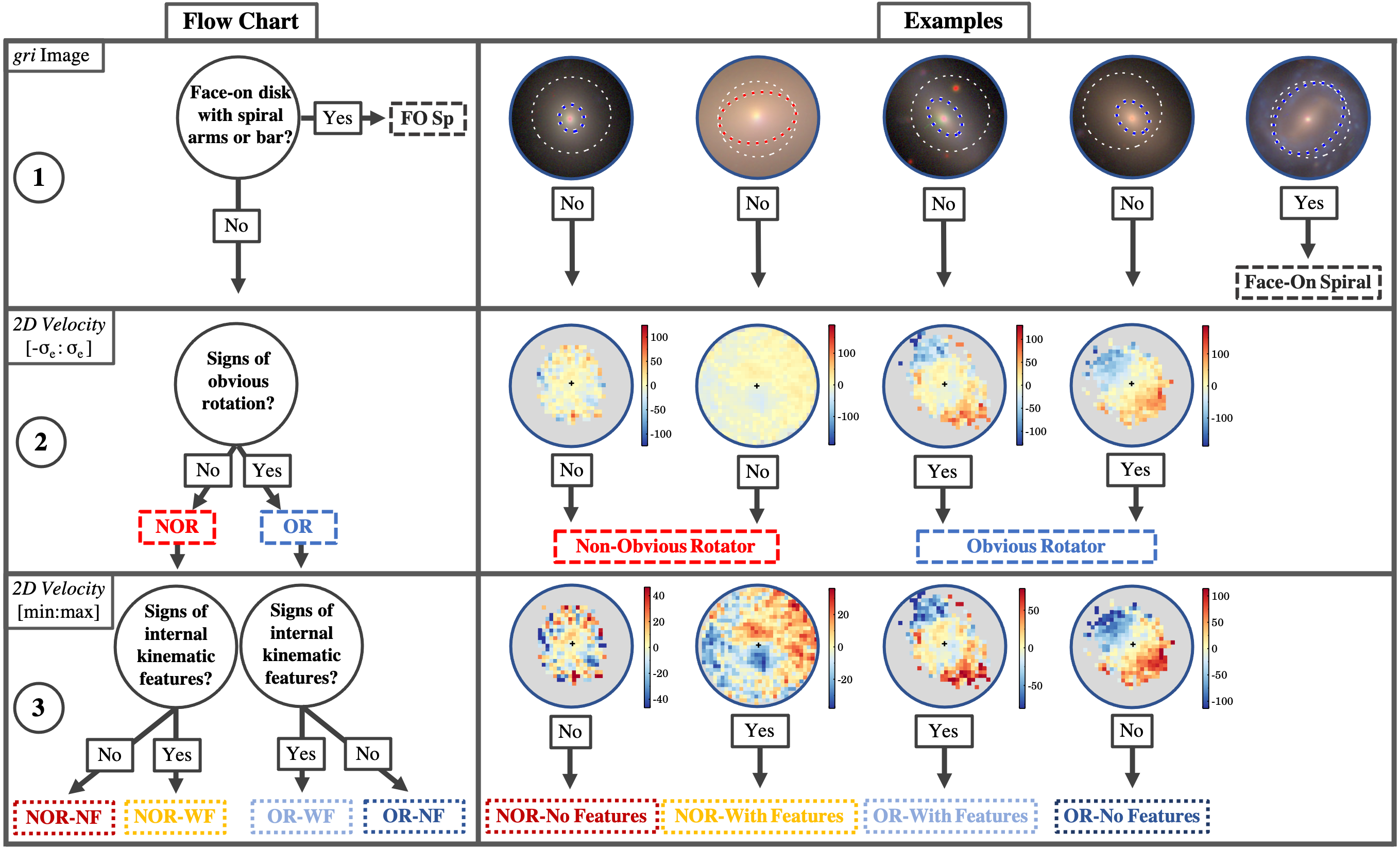
We propose a kinematic visual classification scheme defined as follows (Fig. 5). We begin by defining a specific class for spiral and/or strongly barred galaxies that are close to face-on (FO-Sp), thus showing no obvious rotation. Secondly, we divide the population into "Obvious Rotators" (ORs) and "Non-Obvious Rotators" (NORs). The adopted language is purposely vague to allow for some freedom of interpretation as the classification is qualitative, not quantitative. Whilst the velocity field does not necessarily have to be regular for a galaxy to be classified as an obvious rotator, opposite ends of the velocity field should demonstrate reversed rotation. For the SAMI Galaxy Survey stellar kinematic data, we add one level of refinement. After classifying the kinematic map into OR or NOR, in the third step we check whether the galaxy has an inner kinematic feature ("With Feature"; WF) or not. With improved data quality, this classification scheme can be further refined by adding an extra level to identify the type of kinematic feature (e.g, kinematically distinct core, 2M, etc., from Krajnović et al., 2011).
A flow-chart and five example maps of the different visual kinematic types are presented in Fig. 5. For each galaxy we show the best-available colour image derived from VST-KiDS (de Jong et al., 2017) or Subaru-Hyper Suprime Camera DR1 imaging (Aihara et al., 2018), a velocity map with a range set by the average velocity dispersion, as well as a velocity map with auto-scaling. The first velocity map with -scaling was used to classify galaxies into NORs or ORs, whereas the auto-scaled velocity map is better adjusted for identifying inner kinematic features. The choice for using a velocity range set by the velocity dispersion was motivated by the dependence of the maximum rotational velocity as a function of stellar mass, i.e., the Baryonic Tully-Fisher relation. We also wanted to incorporate the velocity dispersion into the visual classification such that with increasing velocity dispersion the rotational velocity has to become more pronounced in order for a galaxy to be classified as an obvious rotator.
Using similar maps as shown in Fig. 5, seven members of the SAMI Galaxy Survey team visually classified 600 kinematic maps of galaxies with . We chose to visually classify only a selected sample of galaxies, because no NORs were identified at in a test set of 147 galaxies (10 percent of non-classified galaxies). And because kinematic visual classification is time consuming process we only selected galaxies in the region where a mix of ORs and NORs was expected, in order to reduce the total number of galaxies.
Following a similar approach as outlined in Cortese et al. (2016), after all votes were combined, the kinematic type with at least 5/7 votes were chosen (66.7 percent, 399/598). When no absolute majority was found, ORs and ORs-WF were combined into an intermediate type, as well as NORs and NORs-WF. If 5/7 votes then agreed, the galaxy was classified as the intermediate type (23.2 percent, 139/598). For the remaining cases ( percent, 58/598) the classifications of the two most average classifiers were compared and if those agreed that type was chosen (6.2 percent, 37/598). Otherwise, we checked whether a weak majority (4/7) was reached (3.5 percent, 21/598). Only two galaxies in our sample remained unclassified under this scheme.
The results of the kinematic visual classification are presented in the - plane (Fig. 6a-c). Interestingly, we find that the distribution of ORs and ORs-WF extend to very low values of . While this is expected for face-on spirals, we also find ORs-WFs galaxies with low that are classified morphologically as Elliptical and S0s. For NORs, as expected there is an increase in their fraction towards higher stellar mass. The average values of NORs also decrease with increasing stellar mass. We find that low-mass () NORs are nearly all morphologically classified as late-spiral or irregular. In Fig. 6(d) we investigate where ORs and NORs reside in the - plane. The NORs have mostly low ellipticity values, and beyond we only find a handful of NORs. A large fraction of the ORs at low spin-parameter (<0.2) are classified having kinematic features, and similarly for and , which strengthens the argument for setting an ellipticity limit of to select galaxies with actual slow rotation rather than low values due to counter-rotating disks. Note however that face-on galaxies without a strong bar (, ) do not have a measurable rotation and will therefore end up in this SR selection region; these galaxies can only be identified as disk-galaxies from a visual morphological classification.
3.3.2 Identifying Fast and Slow Rotators using Visual Kinematic Morphology as a Prior
Similar to the test we did for kinemetry, we will now treat "Non-Obvious Rotation" as a condition that a galaxy can have, while again using the - diagram as the diagnostic to identify this condition. The confusion matrix is given in Table 2. We then use Equation 6 to select SRs and FRs for an ensemble of selecting regions and calculate the TPR (Equation 2), the FPR (Equation 3), and the MCC (Equation 5). The optimal selection is defined by the highest MCC value.
| NOR | OR | |
|---|---|---|
| SR | True Positive | False Positive |
| FR | False Negative | True Negative |
The TPR versus FPR, and the MCC distribution are shown in Fig. 6(e). According to the MCC parameter, the optimal selection region has shown as the black line in Fig. 6(d), which is close to the from Cappellari (2016). The optimal selection region only has a TPR of 83.1 percent with a small FPR of 3.6 percent, and a PPV of 67.6 percent. If we were to accept a higher FPR of 20 percent, which is reached at , then we obtain an impressive TPR of 98.7 percent, but with an unacceptably low PPV of 30.9 percent. Overall, we conclude that there is a good success of selecting Non-Obvious Rotators and Obvious Rotators using the - diagram. Nonetheless, as the - diagram only shows the average rotational properties within it cannot replace the spatial information obtained through the process of visual classification.
3.4 Using Bayesian Mixture Models for Identifying Different Kinematic Families
3.4.1 Description of the Bayesian Mixture Model
Up to this point, we have been working with the assumption that multiple kinematic populations of galaxies exist. Using kinemetry we separated galaxies into regular and non-regular and for the visual kinematic classification we split galaxies into obvious and non-obvious rotation. Both analyses indicate that the various kinematic classes exist across the full range in stellar masses, with an increased fraction of NRRs and NORs towards high stellar mass. Nonetheless, the question of whether or not a bimodal distribution with two distinct peaks exists has not been answered by this analysis. The distribution from kinemetry only reveals a highly skewed distribution, whereas the visual kinematic classification could be tracing two ends of a continuous distribution.
Here, we are interested in analysing the distribution as a function of stellar mass without forcing two distinct populations, or assuming where these populations should reside in the - plane. To do so, we analyse our data using a Bayesian mixture modelling framework222Inspired by Taylor et al. (2015) who analyse ”blue” and ”red” galaxies as two naturally overlapping populations using an MCMC analysis.. The main assumption we make is that the distribution of galaxies can be well approximated by a beta distribution, where the probability density function (PDF) is given by:
| (7) |
with defined using the Gamma function :
| (8) |
The beta distribution has the property of only being defined on the unit interval, which makes it ideal to describe values of that are also constrained to lie between 0 and 1. However, as the maxima and minima of the observed distributions are not perfectly 0 and 1, we rescale the values in the following way:
| (9) |
To model the locations of galaxies in the - plane, we use a linear combination of two beta functions at each value of stellar mass (which we label 1 and 2). However, the proportion of galaxies which are drawn from each beta distribution at a given stellar mass is not fixed. We allow the "mixture probability" to vary smoothly as a function of stellar mass, which captures the well-known dependence of kinematic morphology and mass (e.g., Emsellem et al., 2011; Brough et al., 2017; Veale et al., 2017; van de Sande et al., 2017a; Green et al., 2018; Graham et al., 2018).
Note that the expected relation of both populations with stellar mass is also the primary reason for not using the - diagram to fit the data. Even though inclination has a significant impact on the observed values that could be partially accounted for by using ellipticity instead of mass, we argue that without an inclination correction we only get an increase in the scatter and overlap of both distributions. While we could attempt to correct for inclination, this parameter is poorly constrained for galaxies below . Only correcting a subset of the data could lead to a bimodality by construction (see Section 3.1), which we want to avoid here. We further investigate the impact of inclination in Appendix C.

At this point, we also apply a volume correction to our cluster sample. The complete volume correction analysis will be presented by van de Sande et al. (in preparation), but we provide a short description here. The SAMI targets are drawn from the volume-limited GAMA survey with high completeness ( percent). However, the GAMA regions lack high over-density regions with halo mass greater than . For that reason the SAMI Galaxy Survey targeted an additional 8 cluster regions to fill this density gap. Nonetheless, the probability of finding an extremely massive cluster such as Abell 85 (the most massive cluster in the SAMI cluster sample) within the GAMA volume is less than one. Hence, a volume correction needs to be applied.
We first calculate the total survey volume, using the stepped series of stellar mass limits as a function of redshift from which the SAMI Galaxy Survey targets were selected (see Bryant et al., 2015). For each volume, we calculate the predicted halo mass function from Angulo et al. (2012) using HMFcalc: An Online Tool for Calculating Dark Matter Halo Mass Functions (Murray et al., 2013). With that halo mass function, we can then obtain a probability of finding a cluster galaxy within the SAMI-GAMA volume. For example, we find that the probability of observing a galaxy in the most massive cluster Abell 85 is . To take this over-abundance of cluster galaxies into account, we randomly draw each galaxy in the full survey - with replacement- using an oversampling of 38 multiplied by a galaxy’s volume correction. In practise, a galaxy in the most massive cluster (Abell 85) will be drawn only once, whereas a galaxy in the GAMA region will be drawn 38 times. For each draw, we add a random number to each data point derived from the measurement uncertainty on and a typical stellar mass uncertainty of 0.1dex. The total volume-corrected dataset consists of 53,587 data points.
We then use this volume-corrected sample to fit the distribution as a function of stellar mass. The shape parameters of both beta functions ( and respectively) are defined to be linear functions of stellar mass. This allows the two beta distributions to vary their width and location in the - plane to match the observational data. Note that the model has the freedom to let one set of parameters have zero contribution if the data do not motivate two populations. A full mathematical description of the model including priors is given in Appendix D.
We fit this model using the python interface to the probabilistic programming language Stan (Carpenter et al., 2017). Stan uses a modified version of the Hamiltonian Monte Carlo algorithm (Duane et al., 1987; Hoffman & Gelman, 2014) to sample the model’s posterior probability distribution and perform full Bayesian inference of the parameters. During the fitting, we run 4 separate chains for 500 warm-up steps and 500 sampling steps each. The warm-up steps are then discarded. We ensure that there are no divergent transitions during the sampling and that the Gelman-Rubin convergence diagnostic (Gelman & Rubin, 1992) for each parameter is within normal values (). Note that no binning in or is applied in the fitting process; each data-point is treated independently.
3.4.2 Probabilistic Fast and Slow Rotators
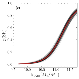
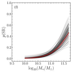
The key results from this analysis are shown in Fig. 7. We identify two clear distributions within the - diagram with moderate overlap. In Fig. 7(a), the blue high distribution, which is consistent with the location of galaxies traditionally called fast rotators, dominates at low and intermediate stellar masses. Above the contribution from a second population at low as shown in red, consistent with traditional slow rotators, becomes more and more dominant towards high stellar mass. While these two populations occupy the exact regions where we expect fast and slow rotators to reside, we want to avoid using the exact same terminology when the process of identifying these two populations is very different from previous studies. Instead, we will refer to these distributions as probabilistic fast and slow rotators (pFRs and pSRs).
In Fig. 7(b), we find that the probability of a galaxy being drawn from the pSR distribution rapidly increases as a function of stellar mass, particularly above , in agreement with previous studies (e.g., Emsellem et al., 2011; Brough et al., 2017; Veale et al., 2017; van de Sande et al., 2017a; Green et al., 2018; Graham et al., 2018). However, the model prediction becomes increasingly uncertain above >11.4 where the number of observed SAMI Galaxy Survey galaxies rapidly drops. The distribution summed over the entire mass range is shown in Fig. 7(c). There is a minor offset of the peak of the pFR distribution as compared to the peak of the data, but the peak of the pSR is well matched to the data.
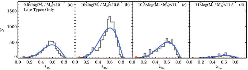
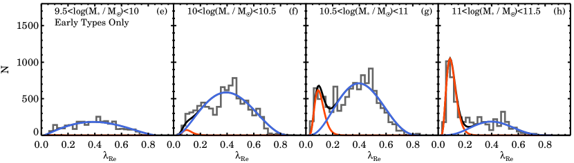
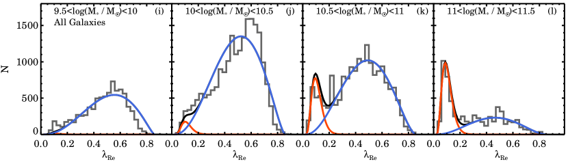
In Fig. 8 we split the sample into four equal bins of stellar mass to investigate this offset further. In particular, we are interested in determining whether or not the main assumption that the distribution can be described by a beta function is valid. Furthermore, we separate the late and early-type distributions because we expect the behaviour of these populations to be different. Indeed, for late-types only, we find that the distribution can be described by a single beta function associated with the pFRs, with minimal contribution of a second beta distribution. However, for early-type galaxies, a second dominant peak appears approximately around , which is also well fitted by a beta distribution.
In the combined sample (Fig. 8 bottom row), we see how the relative contributions of early-types and late-types as a function of stellar mass impact the distribution. Below the late-type population dominates, which is reflected by the strong peak at , whereas towards higher stellar mass the contribution from early-type galaxies becomes more dominant. Between , we find the combined late-type pFR and early-type pFR distribution, which have roughly equal numbers of galaxies, is also well described by a single beta distribution. This is perhaps surprising as the individual late-type and early-type pFR distributions are different in shape with peak values that are offset by in . While this does not exclude that the two populations are kinematically different, it validates the choice of a single beta distribution for the combined early-type and late-type pFR population. We also note that the peak and width of the pSR distributions are identical when analysed as part of the full sample or within the early-type sample. We emphasize that this is not by construction, but an outcome of our mixture model analysis.
Nonetheless, while in three out of four stellar mass bins we find a relatively good fit of our model to the data, in the bin with mass interval we see a poorer fit to the data. The discrepancy between the model and the data could be caused by a relatively high broad peak in the distribution at for late-types, or because we enforce a smooth transition of the beta distributions as a function of stellar mass using a linear relation. Instead, we attribute the poor fit in this mass regime to the lower peak around . The larger abundance of galaxies at these low values could be explained by a population of galaxies that we previously identified as NOR-WF or OR-WF (see Section 3.3). These galaxies might have outer kinematic structures consistent with either the pSR or pFR population, but the inner kinematics offset the measurements from their main distribution. Removing these galaxies from the sample indeed results in a better visual fit, but as our goal here is to use only the spin parameter proxy and stellar mass without secondary identifiers to clean or pre-select our sample, we did not attempt to improve this further.
To summarise, using a Bayesian mixture model analysis we have demonstrated that two beta distributions are required to describe the observed distribution as a function of stellar mass. For early-type galaxies, the location of pFR peak has a lower value as compared to pFR late-type galaxies, but the locations of the pFR and pSR peaks do not change with stellar mass. The amplitude of pSR distribution rapidly increases with stellar mass, but the peak and width remain constant. When we analyse the full SAMI Galaxy Survey sample, we find that the data are well-described by two beta distributions, but because the relative fraction of late and early-type galaxies changes as a function of stellar mass, we also find that the width and peak of the pFR distributions change moderately. These results are consistent with the findings of Guo et al. (2020), who show that in the local Universe, above , both late- and early-type populations become important in the total stellar mass budget, whereas below only one population is needed to reproduce the stellar mass function of galaxies.
| pSR | pFR | |
|---|---|---|
| SR | True Positive | False Positive |
| FR | False Negative | True Negative |
3.4.3 Identifying Fast and Slow rotators using Bayesian Mixture Models as a Prior
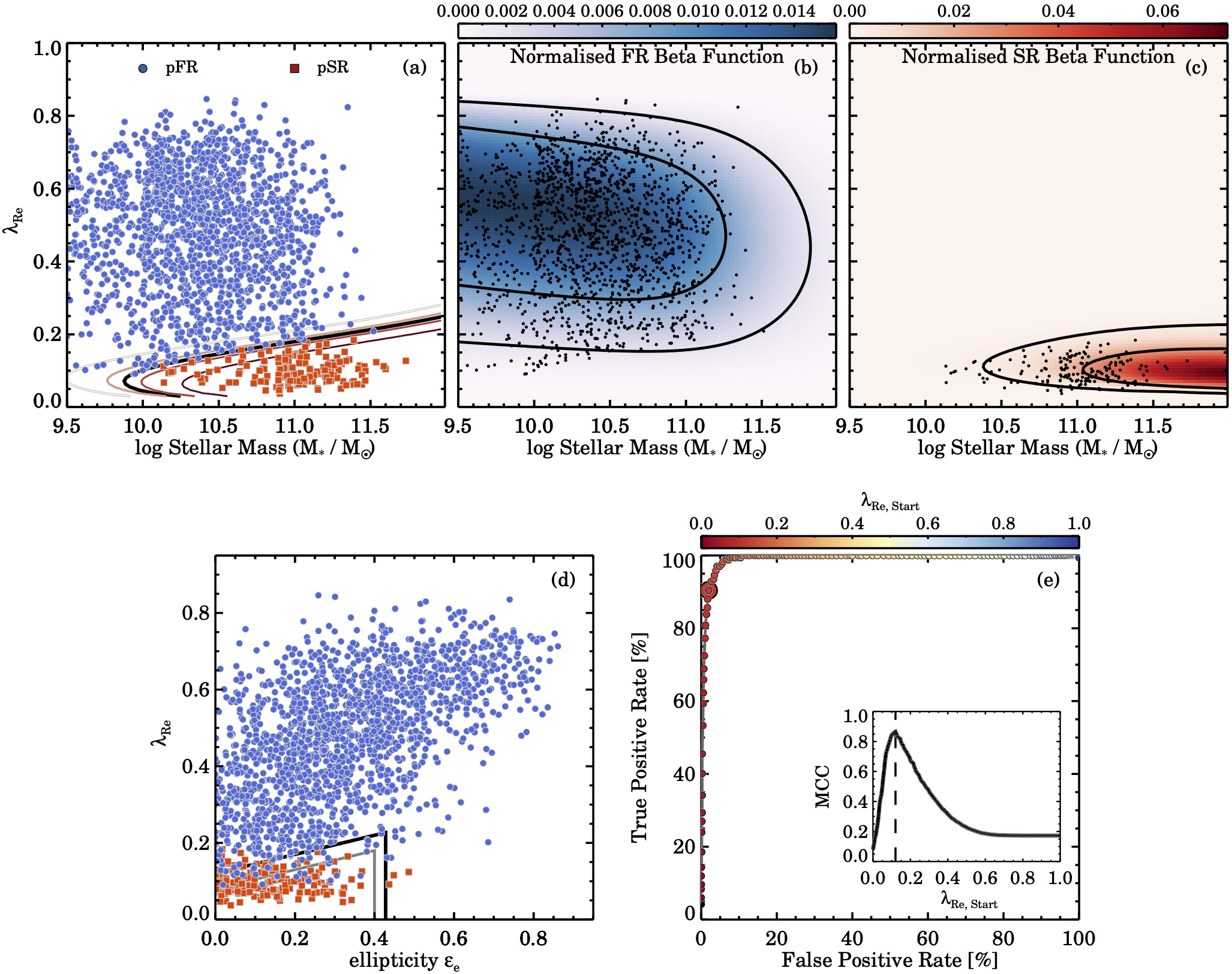
We now use the Bayesian mixture model to identify which galaxies are most likely pFRs and pSRs. In Fig. 9(a) we show the SR probability contours, where . We define a galaxy as a pSR when the is higher than 50 percent. Note that this selection does not take into account ellipticity or visual morphology. For that reason, counter rotating disks that are often excluded using an ellipticity cutoff, or face-on spirals can still be selected as pSR when they are clearly different in structure and kinematics as compared to massive-triaxial ellipticals. We find that the fraction of pSRs strongly increases with stellar mass, which was already demonstrated in Fig. 7. But, the pSR contours are more tightly packed in the direction, whereas the stellar mass range from the 20th to 80th probability covers nearly a dex in stellar mass.
In Figs 9(b) and (c) we show the mass normalised FR and SR PDFs. The contours indicate the 68 and 95 percentiles or how likely we are to find a pFR or pSR in that region. We overlay the SAMI Galaxy Survey data to identify low probability pFR and pSR galaxies. For example, in Fig. 9(b) below there are a number of pFR galaxies that lie below the 95 percentile contours. In our visual kinematic classification analysis (Fig. 6) we already found that this region is predominately occupied by OR-WF, whereas the majority of OR have no such feature. Similarly, we find low-mass pSRs that are outside the 95 percentile. However, whereas the PDFs are normalised as a function of stellar mass, the SAMI observed mass function peaks around . It is therefore no surprise that we find more pSR at than the PDF from a flat stellar mass distribution suggests.
Similar to the test we performed for kinemetry and the visual kinematic classification, we will now treat pFR versus pSR as a condition that a galaxy can have, with - diagram as the diagnostic to identify this condition. The confusion matrix is given in Table 3. In Fig. 9(d) we investigate where pFRs and pSRs reside in the - plane. Unsurprisingly, there is a clear separation between both classes because the pFR and pSR classifications come directly from the - probability cutoffs. Therefore, we are mainly gauging how much overlap of the pFR and pSR distribution there is when swapping for . While this may seem somewhat artificial, we note that both kinemetry and the kinematic visual classification are also based on the kinematic data. Thus, all kinematic identifiers have some degree of interdependence.
We find no dependence on the location of pSR with respect to the ellipticity (Fig. 9d), and in particular towards low , we do not detect a decline in the values of pSR. This result is similar to the NOR category defined from visual classification. To quantify this trend, we explore different selection boxes with varying slopes, start and end positions in both and . Indeed, the optimal selection function has a nearly flat slope starting at =0.14 and extends out =0.5, with an MCC value that is higher than the MCC value from the default selection region from Eq. 6 (0.890 vs. 0.865, respectively).
In Fig. 9(e) we show the TPR versus FPR of our test as well as the MCC distribution for the default selection region region from Eq. 6. The optimal selection only has value of 0.12, with a TPR of 90.4 percent with a small FPR of 1.9 percent, and a PPV of 83.0 percent. Overall, there is an excellent agreement between the selection of probabilistic fast and slow rotators using the - diagram, although we re-emphasise that this is mostly by construction.
4 Different Kinematic Distributions in Cosmological Hydrodynamical Simulations
Cosmological hydrodynamical simulations offer great insight into the formation and evolution of galaxies from high-redshift () to the present-day (). By simultaneously comparing structural, dynamical, and stellar population measurements from simulations and observations, van de Sande et al. (2019) demonstrate that recent large cosmological simulations are now capable of reproducing many of the known galaxy relations. While recent comparisons with IFS measurements showed a qualitatively good agreement for several fundamental galaxy relations (see e.g., Penoyre et al., 2017; Schulze et al., 2018; Lagos et al., 2018b; Choi et al., 2018; Walo-Martín et al., 2020; Pulsoni et al., 2020), quantitatively some fundamental parameters are not well reproduced (Lange et al., 2016; van de Sande et al., 2019; Xu et al., 2019); moreover, areas of discrepancy and agreement vary between the different simulations (van de Sande et al., 2019). Nonetheless, these simulations are useful to interpret the kinematic properties of different galaxy populations across time and different environments (Teklu et al., 2015; Dubois et al., 2016; Welker et al., 2017; Remus et al., 2017; Penoyre et al., 2017; Choi & Yi, 2017; Kaviraj et al., 2017; Choi et al., 2018; Lagos et al., 2018a, b; Schulze et al., 2018; Martin et al., 2018; Pillepich et al., 2019; Walo-Martín et al., 2020; Pulsoni et al., 2020; Schulze et al., 2020).
To assess whether observational selection criteria can be successfully applied to data from simulations to separate fast and slow rotators, we will now repeat the mixture model analysis on IFS mock-observations from cosmological hydrodynamical simulations. We use the data as presented by van de Sande et al. (2019) where we used the eagle, horizon-agn, and Magneticum Pathfinder simulations. All simulations model key physical processes of galaxy formation, including gas cooling, star formation, feedback from stars and from supermassive black holes, although each simulation adopts different philosophies for calibrating to and reproducing observational results. The details of the simulations and mock-observations are summarised below.
4.1 EAGLE and Hydrangea
From the publicly available eagle project (Evolution and Assembly of GaLaxies and their Environments; Schaye et al., 2015; Crain et al., 2015; McAlpine et al., 2016) data, we use the reference model Ref-L100N1504 that has a volume of (100 Mpc)3 co-moving. We combine eagle with hydrangea that consists of 24 cosmological zoom-in simulations of galaxy clusters and their environments (Bahé et al., 2017) to provide a better environmental match to the observed SAMI Galaxy Survey. hydrangea is part of the larger Cluster-eagle project (Barnes et al., 2017). Cluster-eagle is similar to eagle but with different parameter values for the active galactic nuclei (AGN) feedback model, to make it more efficient. Both eagle and hydrangea adopt the Planck Collaboration XVI (2014) cosmological parameters (=0.307, , km s-1 Mpc-1). Each dark matter particle has a mass of , and the initial gas particle mass is . The typical mass of a stellar particle is similar to the gas particle mass. In what follows, we will refer to the joined eagle and hydrangea sample as eagle+.
4.2 Horizon-AGN Simulations
The second set of cosmological hydrodynamic simulations is horizon-agn with the details presented by Dubois et al. (2014). Here, we use the simulation box with a volume of (142 Mpc)3 co-moving with an adopted cosmology that is compatible with the Wilkinson Microwave Anisotropy Probe 7 cosmology (=0.272, , km s-1 Mpc-1; Komatsu et al., 2011). horizon-agn uses a grid to compute the hydrodynamics, employing adaptively refinement to the local density following a quasi Lagrangian scheme (Teyssier, 2002), with cells that are 1kpc wide at maximal refinement level. The dark matter particle mass is , and the adopted resolution is such that the typical mass of a stellar particle is .
4.3 MAGNETICUM Simulations
The third set of cosmological hydrodynamical simulations that we will use are the Magneticum Pathfinder simulations (www.magneticum.org), hereafter simply magneticum (see Dolag et al., in preparation, Hirschmann et al. 2014 and Teklu et al. 2015 for more details on the simulation). We use the data from the medium-sized cosmological box (Box 4) with a volume of (68 Mpc)3 co-moving at the ultra high resolution level. magneticum adopts a cosmology compatible with the Wilkinson Microwave Anisotropy Probe 7 cosmology (=0.272, , km s-1 Mpc-1; Komatsu et al., 2011). The dark matter and gas particles have masses of respectively and , and each gas particle can spawn up to four stellar particles.
4.4 Mock Observations
The method for extracting kinematic measurements from eagle+ are described in Lagos et al. (2018b), for horizon-agn in Welker et al. (2020), and in Schulze et al. (2018) for magneticum, all corrected to km s-1 Mpc-1. For all simulations, we extract -band luminosity-weighted effective radii, ellipticities, line-of-sight velocities and velocity dispersions, adopting techniques that closely match the observations. The values for horizon-agn and magneticum are derived using Eq. 1, whereas for eagle+ we use the definition as described in Emsellem et al. (2007). Note that these different definitions do not impact our analysis as we are investigating the separation of two kinematic families within each distribution, without a direct quantitative comparison. Specifically, the different definitions will only significantly impact galaxies with high values of ellipticity, well above the region where both kinematic distributions are expected to overlap.
A lower mass limit of is used for eagle, hydrangea, and horizon-agn, but a higher mass limit of for magneticum, to ensure that the simulated measurements from the mock-observations are well-converged. Nonetheless, we acknowledge that with the spatial resolution of these simulations, effects similar to observational beam-smearing might play a role in the kinematic measurements of mock-observed simulated galaxies. Lastly, a mass-matching technique is used to remove the difference between the observed and simulated stellar mass function for a clearer comparison of the results (for more details see van de Sande et al., 2019), but we note that we find consistent results when no mass-matching is enforced.

4.5 Separating Fast and Slow Rotators in Simulations using Bayesian Mixture Models
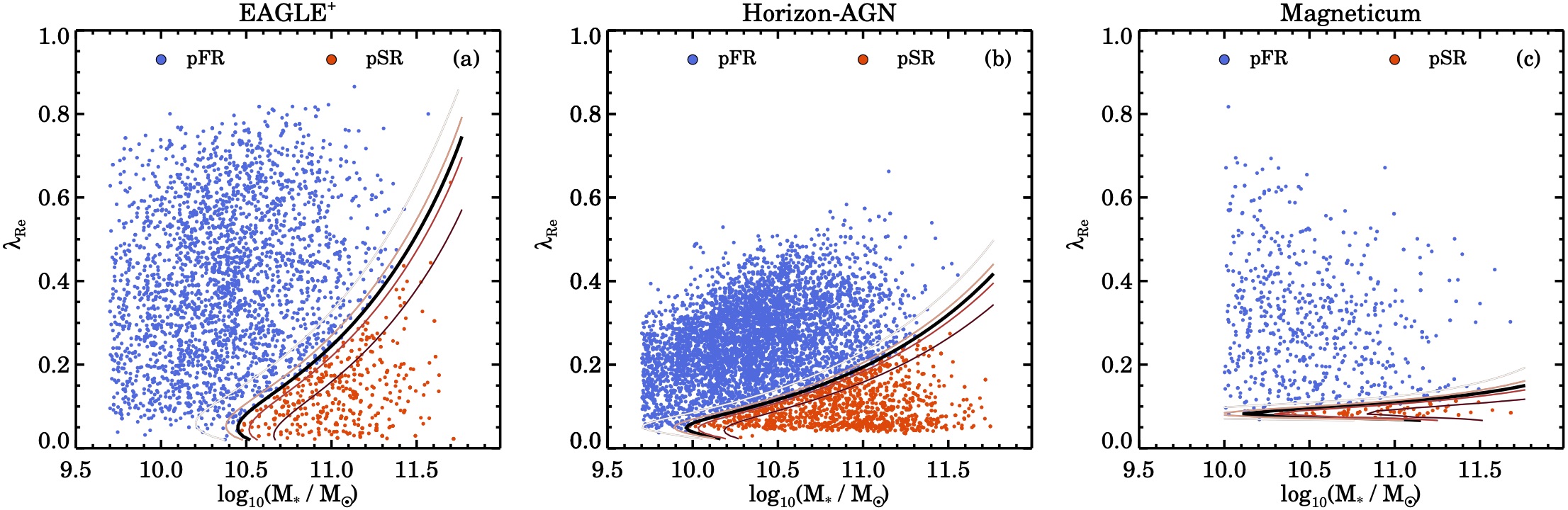
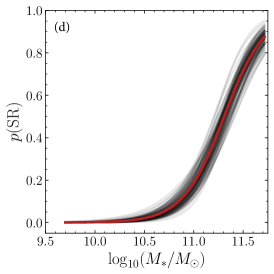
We now repeat the Bayesian mixture model analysis from Section 3.4. Our goal is to see whether or not our mixture model recovers a meaningful separation of the two kinematic distributions within the simulated data, even though we have not demonstrated yet that two kinematic populations exist. The results for all three simulations are presented in Fig. 10, with the left column showing the eagle+ analysis, horizon-agn in the middle column, and magneticum on the right-hand side. We present the separation of pSRs (red) and pFRs (blue) using the 50 percent probability levels in the top row, whereas the bottom row shows the probability of being drawn from the pSR beta distribution.
The difference in the location of the pSR population is striking for all three simulations. As compared to pSR selection region from observations, we detect a steeper upturn in towards high stellar masses for horizon-agn and even steeper for eagle+. In contrast, the magneticum pSR contours increase much slower as a function of stellar mass, with a narrow range in permitted values, although the upper limit of the pSR selection is similar to observations. The other striking difference between the observations and simulations is the location and the shape of the pFR distribution. Below for eagle+ and for magneticum, the pFR distribution covers the full range, whereas for horizon-agn the peak of the pFR distribution is very low from to .
From the probability of the pSR beta distribution as a function of stellar mass (Fig. 10f) it is clear that the Bayesian mixture model for the magneticum simulation data is not as well constrained as compared to the other two simulations and the observed SAMI Galaxy Survey data (Fig. 7). The numerous model realisations indicate that there is a considerable range of possible solutions. The probability of finding the pSRs distribution at the highest stellar masses in magneticum is also lower as compared to the observations (respectively, 0.5 versus 0.75), whereas eagle+ and horizon-agn predict consistent values. Furthermore, in Fig. 10d)-e) we find that for eagle+ and horizon-agn the p(SR) as a function of stellar mass are similar. It is not obvious that this should be the case, especially given the large differences in the ranges of from the two simulations (Fig. 10a-b).
In order to see how well the mixture model separates the pSR and pFR distributions in the simulations data, we present the distributions in different stellar mass bins in Fig.11. We find a wide variety of distributions, both in terms of shape and maximum extent. Most noticeably for eagle+, and to a lesser extend in horizon-agn, we find that the width of the pSR distribution increases with increasing stellar mass, with a tail towards higher and higher even though the peak of the pSR distribution remains at the same location. However, for magneticum the pSR distribution is extremely narrow and does not change considerably as a function of stellar mass.
In all three simulations the mixture model suggests a bimodal distribution, even though two distinct peaks are not evident for each simulation in Fig.11. While this does not imply that multiple kinematic populations do not exist, it does demonstrate the value of investigating the kinematic distributions beyond the work as presented in van de Sande et al. (2019). Here, we find that the overlap between the pSR and pFR distributions is more considerable in the simulations as compared to observations, and that the dividing line for pSR and pFR is at different values as a function of stellar mass. Thus, a good agreement between the observed and simulated distributions does not automatically imply that the ratio of sub populations matches as well. These results also show that the observational selection criteria that are used to classify galaxies into fast and slow rotators are not suitable to study the fractions of the simulated populations as a function of stellar mass or environment. Within the same SR selection region, between observations and simulations it is unlikely that a comparable population of galaxies will be selected without considerable contamination.
5 Discussion
The taxonomy of galaxies determined from their visual morphological properties has been a powerful tool to advance our knowledge of the processes that shape galaxies, with the Hubble Sequence (Hubble, 1926) and the De Vaucouleurs system (De Vaucouleurs, 1959) still in active use today. However, like any other area where taxonomy is used, an introduction of hard boundaries between classes can create artificial dichotomies when in reality the transition between these classes could be continuous 333See Graham (2019) for a detailed discussion on the ”artificial division of the early-type galaxy population” from size measurements..
With increasingly large samples of galaxies with resolved kinematic measurements, various kinematic classifications have now been proposed. Some of these naming conventions have perhaps led to an oversimplification of the way we view the kinematic galaxy population with an assumption that the previously proposed classes are distinct and independent. In this paper, we have investigated how well we can separate a bimodal kinematic distribution in the galaxy population, specifically when the data quality is more severely impacted by seeing and spatial sampling. In the second half of this analysis, we convincingly show that we can separate two kinematic populations, yet when relying on secondary classifiers such as kinematic visual classification or kinemetry we find that the overlap of these different classes can be considerable. Because of the mixing of the different distributions, we are cautious to assign individual galaxies to a certain class. Instead, we advocate using probabilities to assess how likely it is that galaxies share the same properties. Nonetheless, historically various kinematic tracers have been used to promote the existence of a dichotomy. These will be reviewed in Section 5.1-5.5, whereas the implications of our work are discussed in Section 5.6-5.7.
5.1 Separating Fast and Slow Rotators based on Visual Kinematic Classification
We will start with a historical context on the visual kinematic identification of the first resolved kinematic maps that formed the foundation of the work that we present in this paper. Kinematic visual classification only became advantageous with the introduction of the SAURON IFS (Bacon et al., 2001), followed by several IFS surveys. But, as we will argue in this section, the lack of a clear and well-defined classification scheme and the limited field of view has made kinematic visual classification overly subjective with some key results left open to alternative interpretations.
The SAURON survey (de Zeeuw et al., 2002) yielded kinematic maps for a significant sample of 48 nearby early-type galaxies. A visual analysis revealed that most early-type galaxies show a significant amount of rotation, whereas others have complex dynamical structures inconsistent with being simple rotating oblate spheroids (Emsellem et al., 2004). Visual classification of the kinematic maps was further explored in Emsellem et al. (2007) and Cappellari et al. (2007) who introduced the fast and slow rotator classes. However, a detailed look at some of the early results suggests that even with good quality data, the classification is not always obvious. For example, we would argue that from fig. 1 in Emsellem et al. (2007), it is not clear that elliptical NGC 5982 (2nd row, 6th column) is a slow-rotator galaxy as the outskirts show rapid rotation. In our revised kinematic classification scheme from Section 3.3 this galaxy would be classified as an obvious rotator with features (OR-WF).
Similar ambiguities can be found in the kinematic maps from the ATLAS3D Survey using the SAURON IFS, as presented in fig. 1 from Krajnović et al. (2011). For example, galaxies NGC 4472 and NGC 4382 are classified as NRR-CRC (Counter-Rotating Core) and RR-2M (Double Maxima), respectively. From kinemetry the classification into NRR and RR is clear: for NGC 4472 and for NGC 4382. However, when attempting a visual classification of the velocity fields, we would argue that these velocity fields in the outskirts do not look that different, where there are clear signs of rapid ordered rotation. Both galaxies are round (=0.17, 0.2) and have respective values of 0.08 and 0.16, which puts them well-below and relatively close to the fast/slow rotator dividing line (SRs must have <0.14 at =0.20). Combined with the fact that both velocity fields do not extend beyond 0.26-0.36, it is hard to argue that one galaxy is a clear slow rotator whilst the other is not.
Our revised kinematic classification scheme was purposely designed to take into account such ambiguity by adopting a new terminology of "obvious" and "non-obvious" rotation (ORs and NORs). Even though the extent of the kinematic maps is still important, outer versus inner rotation is more clearly defined in this revised scheme (see also Section 5.4). Additionally, our SAMI kinematic sample has at least one kinematic coverage for percent of the galaxies, and only a relatively small fraction of galaxies do not extend beyond 0.5 ( percent).
The new visual classification scheme also allows each user to come up with their own interpretation of what ORs and NORs could look like, although we offer some examples of what the classes might look like. "Self-calibration" is important in this classification scheme, and to facilitate this, each classifier was shown their collection of galaxies assigned to the same class after each subset. By being allowed to swap galaxies between classes, the most optimal selection could be made. Given this ambiguity and flexibility in the classification scheme, the bimodal distribution of ORs and NORs in the - space (Fig. 6) is surprisingly clear, and confirms that two classes indeed exist.
Unlike some previous classifications (Graham et al., 2018), we advocate for the aggregation of classifications from many independent classifiers. A comparison of visual classifications from three different authors on the SAMI maps, using the classifying scheme from Krajnović et al. (2011), resulted in a large range in classification, with poor overall agreement. Results based off single classifiers may thus be biased and artificially skew the resulting distributions. A supervised machine learning approach (e.g., boosting), or a citizen science project (e.g., Galaxy Zoo; Lintott et al., 2008), could provide a viable solution for the near future when the number of galaxies with 2D kinematic maps is expected to grow beyond 10,000. We further emphasise that a more quantitative approach guided by these visual classifications should always be sought to connect to other studies and simulations
5.2 Separating Regular and Non-Regular Rotators using Kinemetry
kinemetry offers a quantification of the irregularity of the velocity field (Krajnović et al., 2006; Krajnović et al., 2008, 2011) and has been exploited to classify galaxies into Regular and Non-Regular classes. This classification scheme formed the basis for the revised - separation line of fast and slow rotators in Emsellem et al. (2011) and Cappellari (2016). We re-analyse the separation of ATLAS3D fast and slow rotators using our ROC analysis (see Appendix B.1) and find a clean separation of RR and NRR with a high Positive Prediction Value (89.7), but with an optimal selection region that has a higher limit as compared to Emsellem et al. (2011) or Cappellari (2016).
Nonetheless, using a sub-set of high-quality SAMI Galaxy Survey data, van de Sande et al. (2017b) showed that the distribution from both ATLAS3D and SAMI was peaked around but with a continuous tail towards higher values. Yet, the shape of this distribution does not suggest that the distribution in is bimodal. Furthermore, in Section 3.2 we show that with lower quality data, the overlap of regular and non-regular galaxies in the - and - space is considerable. As is intrinsically correlated with and through the rotational component, galaxies with high or values will always have lower if the component remains constant. Thus, while kinemetry provides a useful and quantifiable measure of the kinematic asymmetry of the velocity field, we argue that this method does not provide strong evidence for a kinematic dichotomy.
5.3 Separating two kinematic families using JAM Modelling
Using Jeans Anisotropic MGE (JAM) modelling of ATLAS3D galaxies (Cappellari et al., 2013b), Cappellari (2016) shows that the distribution of is bimodal, where is the ratio of the observed velocity and the modelled velocity from JAM using an oblate velocity ellipsoid. Regular rotators are Gaussian distributed around , whereas non-regular rotators conglomerate towards zero, with minor overlap of both distributions (see also 14c).
In Appendix B.2 we repeat our ROC analysis with ATLAS3D data using as the identifier for slow rotators. We only find a marginal improvement of the MCC parameter if we use JAM modelling as compared to using kinemetry. Further, as noted by Cappellari (2016), for non-regular rotators without a disk "the shape of the predicted is, even qualitatively, very different from the observed velocity field." JAM models assume axisymmetry, so perhaps it is unsurprising that triaxial ETGs have low values of . Nonetheless, dynamical modelling clearly shows that there is a family of galaxies consistent with being axisymmetric oblate rotating spheroids, and a class of galaxies with more complex dynamical properties that are not well-fitted by Jeans models. Schwarzschild modelling (Schwarzschild, 1979), has great potential for understanding the orbital structure of all types of galaxies (see for example van den Bosch et al., 2008; van de Ven et al., 2008; Zhu et al., 2018a, b, using SAURON and CALIFA IFS data). Yet, the technique remains computationally expensive and requires high-quality data for the orbital decompositions to be non-degenerate.
5.4 The impact of a Radial Extent on the Slow Rotator Classification
The radial extent out to which the kinematic measurements are analysed also has a significant impact on the fast and slow rotator classification. When visually classifying kinematic maps, more attention may subconsciously be given to larger radii, with the eye being drawn to the larger number of spaxels in the outskirts. This is one of the reasons why our revised classification scheme distinguishes between obvious versus non-obvious rotation, which can be more easily picked up in the outskirts, with a refinement option for kinematic features towards the centre. Nonetheless, if the radial coverage of the kinematic maps do not extend beyond the central region (e.g., ), the classification will be inherently biased.
For quantitative measurements, a scale of one is typically adopted because of observational constraints that are necessary to obtain the required S/N ratio to extract the LOSVD beyond this radius. However, there is no physical reason to restrict our kinematic measurements to within this radius and this approach might have hampered our understanding of galaxies (e.g., see Graham, 2019). The radial coverage varies considerably between different IFS surveys, but more importantly, it typically changes as a function of stellar mass within surveys as well. The necessity for aperture-correcting and measurements is demonstrated in van de Sande et al. (2017a) (see also D’Eugenio et al., 2013) who show that there is a strong bias in the largest measurable kinematic radius as a function of stellar mass, which significantly impacts the fraction of slow rotators.
Studies measuring the kinematic parameters out to larger radius have demonstrated that the rotational properties of galaxies can change when measured at a different radius (e.g., Weijmans et al., 2009; Proctor et al., 2009; Arnold et al., 2011). More recently, radial tracks within the space have been utilised to study how the radial kinematic behaviour changes using increasingly large samples (Graham et al., 2017; Bellstedt et al., 2017; Foster et al., 2018; Rawlings et al., 2020). Kinematic full-spectral bulge–disk decomposition now also offer the possibility to explore for bulges and disks separately (Tabor et al., 2017; Méndez-Abreu et al., 2018; Tabor et al., 2019; Oh et al., 2020). For a single kinematic galaxy classification that is based on an average quantity such as , a larger aperture will always be preferred to include the largest possible fraction of stellar mass. But for classifying internal sub-components the aforementioned methods will be essential. While several past (e.g., SLUGGS, Brodie et al. 2014; CALIFA, Sánchez et al. 2012) and upcoming (e.g., Hector Bryant et al. 2016; MAGPI, Foster et al. 2020) IFS surveys are aimed at providing larger coverage, for the coming years the largest samples of galaxies will still be restricted to 1-2.
Therefore, well-calibrated large cosmological simulations will be crucial to offer insight into the build-up of mass and angular momentum at large radius (e.g., Schulze et al., 2020; Pulsoni et al., 2020) which can be tested observationally with smaller samples that have large coverage (e.g., Sarzi et al., 2018; Gadotti et al., 2019).
5.5 Do Simulations Predict Two Kinematic Families?
Many theoretical studies have tried to explain the origin of the different kinematic classes of galaxies, in particular in relation to the impact of mergers (for a review on the topic, see Naab et al., 2014). While several early-type formation models managed to create galaxies with little rotation, the detailed properties of those simulated galaxies still differ significantly from observations (e.g., Bendo & Barnes, 2000; Jesseit et al., 2009; Bois et al., 2011).
Binary galaxy merger simulations demonstrate that the majority of merger remnants are consistent with being fast rotating galaxies (Bois et al., 2010, 2011), with the mass ratio of the progenitors being a crucial parameter for creating slow rotators, although the orbit-spin orientation of the merger might be as important (Moody et al., 2014). A clear bimodality in - is seen in both Jesseit et al. (2009) and Bois et al. (2011), but Bois et al. (2011) caution that this bimodality "could likely result from the specific choices of simulated mass ratios and the limited number of simulated incoming orbits". The relative importance of a dissipational component in the formation of a bimodal populations is still unclear, with contrasting results from Cox et al. (2006) and Taranu et al. (2013).
Cosmological simulations offer a more realistic insight into the kinematic distribution of modelled galaxies, although the fast/slow selection nearly always follows the observational criteria. In this paper, we demonstrate that considerable differences in the location of the different distributions of fast and slow rotators exist as compared to observations and between simulations. Quantitative offsets in galaxy structural, kinematic, and stellar population parameters were already demonstrated to exist as shown by van de Sande et al. (2019), so it is not surprising that the selection criteria for fast and slow rotators should be adapted for the different simulations.
Nonetheless, the large differences of the pSR populations towards higher stellar mass in the simulations is perhaps surprising. While lower mass galaxies assemble their stellar material primarily though star formation (Robotham et al., 2014), mergers dominate the addition of stellar material in galaxies above () and also are key in lowering angular momentum in galaxies. Large differences between the frequency and mass-ratio of mergers are not expected between different cosmological simulations, which points towards a different problem within the simulations. The key might lie in the fast-rotating population. None of the simulations showed a close match to the observed pFR distribution, and if the progenitors of slow rotators do not match the observed distribution, perhaps we should not expect the pSR distribution to match either.
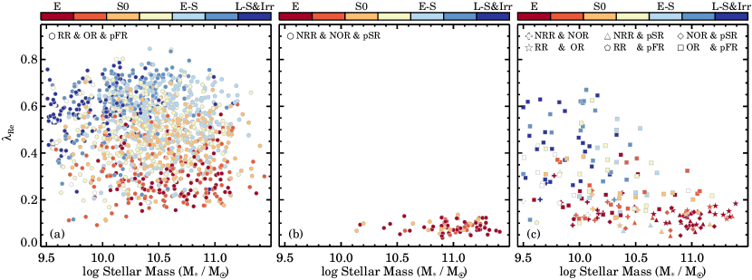
Alternatively, the large differences in the distributions could indicate that the presence and treatment of gas, star-formation, as well the feedback subgrid models in these simulations are more critical for the kinematic properties of all galaxies than previously assumed, although the effects could be indirect. The exact prescription for how feedback is modelled will change the abundance of gas in galaxies and will therefore impact the frequency in which dry versus wet mergers happen as well as their typical mass ratios (e.g., see Dubois et al., 2013, 2016; Lagos et al., 2018a). Both of these factors are important in the formation of slow rotators. This idea is in contradiction with the finding from Penoyre et al. (2017) who conclude that no major difference is found due to presence of gas in mergers in illustris, whereas Naab et al. (2014) using cosmological zoom-in simulations, and Lagos et al. (2018a, b) using eagle, found a clear impact of the gas content on galaxy spin. The latter results are also confirmed by Martin et al. (2018) who find that the morphology of merger remnants strongly depends on the gas fraction of the merger and that re-grown disks are common in gas-rich mergers. However, as no clear picture into the formation of slow rotators has yet emerged from large-volume cosmological simulations, it will be paramount to accurately compare distributions of observations and simulations in consistent ways.
5.6 How To Best Separate Two Kinematic Families
The main aim of this paper is to investigate how we can best separate different kinematic populations and to what extent these different kinematic populations overlap. In our analysis, we have investigated three kinematic classifications in detail (kinemetry, visual kinematic morphology, and Bayesian mixture model classification), but have not yet directly compared the different classifications to each other. We address this here by looking at the agreement and disagreement between these methods. We select galaxies which have all three classifications, which reduces the total sample from 1765 to 1625 galaxies, caused by the fact that not all galaxies have measurements out to one . Galaxies are then grouped according to where their classifications agree: 1) a galaxy is an RR, an OR, and a pFR (Fig. 12a), or 2) a galaxy is an NRR, an NOR, and a pSR ( Fig. 12b), or 3) a galaxy only has two out of three matching classifications (Fig. 12c). It should be noted that none of the kinematic identifiers used here are truly independent as they all rely on the velocity and velocity dispersion maps.
The overlapping FR classifications form the biggest group with 82.6 percent (1342/1625), the SR classifiers are the smallest (4.8 percent; 78/1625), whereas galaxies with mixed classifications make up 12.6 percent of the total sample (205/1625). Within the mixed classified sample, the largest subgroup is where galaxies are classified as ORs and pFRs, but where kinemetry suggests the galaxies are NRRs (114/205). As most of these galaxies reside towards lower stellar masses and higher we argued before that the high values that lead to this classification are more likely caused by observational effects rather than their intrinsic properties. This suggests that when using kinemetry with SAMI-like data quality, the NRR population has the highest probability to be contaminated with ORs and pFRs.
We conclude that the visual kinematic morphology and the Bayesian mixture model analysis provide the most consistent classification. Using a modified version of the Cappellari (2016) slow rotator selection region, we also find a high positive predictive value for separating the NOR/OR and pSR/pFR classes. Therefore, a combination of the two methods with the associated selection box is recommended for selecting SRs from the SAMI Galaxy Survey or data with similar quality when aiming to compare to previous studies that separate fast and slow rotators.
5.7 Implications for Galaxy Formation Scenarios
A critical stellar mass limit of has been proposed as the limit above which passive slow rotators with cores dominate (see discussion in Cappellari, 2016), to the point where galaxies below this mass limit are no longer classified as slow rotators (Graham et al., 2019). Although our data quality does not allow us to address the question of whether slow rotators in our sample have core or power-law inner light profiles, we do not find evidence for a limit below which there are no NNRs, NORs, or pSRs, as based on kinemetry, visual kinematic classification, or the Bayesian mixture models. Depending on the kinematic galaxy identifier (e.g., kinemetry, visual classification, Bayesian mixture models) we find the fraction of these different populations to start rising at different stellar masses. The analysis from Falcón-Barroso et al. (2019, fig. 5) using CALIFA data also clearly shows a group of slow-rotator ellipticals with stellar masses below . Furthermore, some of the cosmological simulation data analysed here also reveal a small, but non-negligible fraction of slow rotators towards low stellar mass. Hence, we are cautious to use mass as a selection criterion for slow rotators, in particular when their formation process is still not well understood.
One of the striking results from our Bayesian mixture model analysis is that the peaks of the pFR and pSR distributions are nearly constant as a function of stellar mass. While this appears to be in conflict with the general notion that galaxies have lower with increasing stellar mass, our results indicate that this kinematic trend is caused by a changing fraction of galaxies in the pFR and pSR distribution. Towards higher stellar mass, the fraction of galaxies in the pFR decreases while it increases for the pSR, leading to a lower of the entire population.
The constant peak for pSRs as a function of stellar mass implies that the formation process of SRs, i.e., the near complete removal of a galaxy’s angular momentum, is likely similar across all stellar masses. If the mechanism transforming pFRs into pSRs was different as a function of stellar mass, we would either observe a different pSR peak, or a change in the width of the pSR distribution. We detect neither. Nonetheless, the strong fractional increase of the pSRs distribution as a function of stellar mass may indicate that the SRs formation process is more efficient towards higher stellar mass, or else that the processes which cause a galaxy to evolve into a slow rotator also tend to lead to it becoming very massive. This picture is consistent with predictions from cosmological simulations that show that approximately 30-50 percent of the SRs are produced in a single massive merger (e.g., Schulze et al., 2018; Lagos et al., 2020), a process that can happen at all stellar masses, albeit it is most efficient in transforming galaxies into slow rotators if the merger is dry, which is more likely at higher masses.
These predictions can be tested with enhanced number statistics combined with better kinematic data quality (e.g., Hector, Bryant et al., 2016) or by going to higher redshift (e.g., MAGPI at , Foster et al. 2020; LEGA-C at , van der Wel et al. 2016). Early results from the LEGA-C survey indicate that there is increased rotational support in quiescent galaxies (Bezanson et al., 2018), although it’s not clear yet whether this is due to a change in the or peak of the pFR and pSR distributions or a change in the fractions of pFRs and pSRs distributions.
6 Conclusion
The dynamics of galaxies offers great insight into the assembly and redistribution of stellar mass within galaxies over time. The prevailing physical explanation for drastically altering the dynamical properties of galaxies is undoubtedly merging and accretion. Yet many questions still remain on the importance of gas as a dissipational component as well as the frequency of major and minor mergers and their impact on the inner and outer stellar distributions. Key to answering these questions is identifying the different kinematic populations that exist and link these to the various proposed formation scenarios.
Using data from the SAMI Galaxy Survey we investigate whether or not we can detect a bimodality in the kinematic properties of the entire galaxy population using versus stellar mass and ellipticity. The main goal of the paper is to use different techniques to identify whether we can accurately separate a bimodal kinematic distribution in relatively low-signal-to-noise, seeing-impacted data, and to what extent different kinematic populations overlap. By doing so, we aim to consolidate results from ongoing multi-object IFS surveys with the conclusions from previous IFS surveys that had better S/N and spatial resolution, but where the sample size did not allow a statistical analysis. We also provide a framework for comparing these results to mock-observations from cosmological simulations.
We find the following results:
(i) Partially applied seeing corrections can lead to an artificially enhanced bimodality. Using 1765 SAMI galaxies with measurements we investigate the impact of the seeing corrections. No clear bimodal distribution in is detected in the SAMI seeing-dominated data or when the Harborne et al. (2020a) correction is applied to all galaxies (Figs 3a and c). However, when only regular rotators are seeing-corrected, as was done in Graham et al. (2018), we detect a clear bimodal distribution in , but we argue this is an artificial construct as the correction is applied to a subset of the sample (Fig. 3b). Thus, from the - diagram alone using SAMI Galaxy Survey data, we do not find strong evidence for distinct kinematic populations of galaxies.
(ii) There is considerable overlap of regular and non-regular rotator distributions with SAMI. With galaxies classified as regular and non-regular rotators from the kinematic asymmetry of the rotational velocity fields using the kinemetry method, we investigate the amount of overlap of the RR and NRR distributions within the - and - diagrams. At low stellar mass, NRR (>0.07) have higher values of than at high stellar mass (Figs 4a and c). We find considerable mixing of the regular and non-regular rotator populations in our SAMI sample, in particular below . The trend of decreasing values with increasing stellar mass also leads to considerable overlap of RRs and NRRs within the - diagram. We use a "Receiver Operating Characteristic Curve" (ROC) and "Matthews correlation coefficient" () to determine the best possible selection box to separate RR and NRR within the - diagram. For SAMI Galaxy Survey data the optimal selection region has a higher threshold as compared to the selection box from Cappellari (2016), but overall does not provide a clean separation of regular and non-regular rotator classes as the Positive Prediction Value is only 65.7 percent.
(iii) Visual kinematic classification of SAMI data leads to a cleaner separation of two kinematic populations. We devise a new visual classification scheme that first separates galaxies with obvious rotation (ORs) from galaxies with no obvious rotation (NORs), combined with a second layer of refinement to find galaxies with inner kinematic features (with-features versus no-features). There is a well-defined separation of ORs and NORs within the - and - planes. Similar to kinemetry we find that the NORs have higher values of towards lower stellar mass. The optimal selection region for selecting NORs using and is close to the selection region from Cappellari (2016). Furthermore, the ROC analysis reveals a significantly higher success rate as compared to using kinemetry for SAMI, which suggests that our visual classification scheme is more suitable for data that has a large range of S/N and the typical spatial resolution of SAMI or MaNGA.
(iv) Bayesian mixture models provide the cleanest separation of two kinematic families. Rather than looking for two populations using kinemetry or visual classification, we use a Bayesian mixture model analysis to determine whether multiple populations can be identified as a function of stellar mass. At all stellar masses, the distribution for late-type galaxies is well described by a single beta distribution that peaks at . However, for early-type galaxies above a second beta distribution is required with a lower peak at . These results demonstrate clearly that we can separate two stellar kinematic populations from the distribution, even when these distributions have non-negligible overlap. Based on these results, we then refer to galaxies as probabilistic fast or slow rotators (respectively, pFRs and pSRs). In contrast to NRRs and NORs, pSRs have lower values at lower stellar mass. This could indicate that the NRRs and NORs found at low stellar mass are simply the lower tail of a broad distribution, but not a separate class. Even though pSR have slightly higher values towards high stellar mass, the pSRs and pFRs are extremely well-separated within the -, but with a caveat that pSRs were selected primarily using .
(v) Mixed results from Cosmological Hydrodynamical Simulations. We apply the same Bayesian mixture model analysis to mock-observations from the eagle and hydrangea, horizon-agn, and magneticum cosmological hydrodynamical simulations. Although the mixture model predicts two populations of stellar rotators in all three simulations, the peak of the two beta distributions is significantly offset from observations, and the fraction of both beta distributions as a function of stellar mass also change considerably. The overlap of the two beta distributions also differs significantly between the simulations. Our results indicate that the treatment of the ISM and feedback subgrid models within these simulation have a considerable impact on the distribution of fast and slow rotators. More importantly, observational selection criteria for fast and slow rotators should not be applied to data from simulations to derive the fraction of different kinematic populations unless the distributions in and are well-matched to the observations they are compared to.
(vi) The optimal classification of galaxy stellar kinematics. By comparing three kinematic classification methods (kinemetry, visual kinematic morphology, and a Bayesian mixture model) we find the best agreement between the visual kinematic morphology and Bayesian mixture model classification. Nonetheless, we argue that visual classification provides a unique spatial kinematic insight, and maintains its usefulness for future work. For comparing to previous studies that adopted the Cappellari (2016) selection box to separate fast and slow rotators, we advise using Eq. 6 with when the data quality is similar to that of the SAMI Galaxy Survey. However, we stress that our analysis revealed a significant amount of overlap between the different kinematic distributions which should be acknowledged.
Going forward. Many claims about a kinematic bimodality have been made in the past with an ongoing unquenchable drive to separate galaxies into binary classification. In this paper, we confirm key findings from previous and ongoing IFS studies that the vast majority of galaxies are consistent with being a family of oblate rotating systems viewed at random orientation. At the same time, there is a group of mainly massive early-type galaxies that show complex dynamical structures, irregular velocity fields, 2-sigma peaks, or kinematic misalignment, with indications that some fraction of these galaxies are triaxial systems.
The rapid increase in the number of galaxy IFS observations has been achieved by a compromise between multiplexing, spatial resolution and S/N. Nevertheless, we have demonstrated that we can extract different kinematic populations in seeing-impacted data, but only when the analysis techniques are matched to the data quality. However, even when using higher-quality data (e.g., see Appendix B), with different kinematic identifiers the same galaxy can be simultaneously classified into opposite groups (e.g., a RR-SR or NRR-FR). Our results show that it has become essential to take into consideration that the distributions of various kinematic populations overlap. When the overlap and mixing of classes is ignored, and naming conventions for various kinematic classifications slowly morph into a singular class (e.g., all non-regular rotators are slow rotators and vice versa), the complexity of galaxy evolution is disregarded. Cosmological simulations have shown that galaxy evolution is a highly stochastic process, hence we do not expect distinct, cleanly separated classes. Instead, we promote the analysis of stellar kinematic data using probability distribution functions instead of bimodal classes. With more than 10,000 IFS galaxy observations becoming publicly available soon (e.g., SAMI Galaxy Survey, SDSS-IV MaNGA), now is the perfect time to further pursue such an endeavour.
Acknowledgements
We thank the anonymous referee for their thorough and thoughtful comments that have improved the clarity of this paper. We also thank Tim de Zeeuw and Michele Cappellari for insightful and helpful comments on the paper, and thank Alister Graham for useful discussions on this topic. The SAMI Galaxy Survey is based on observations made at the Anglo-Australian Telescope. The Sydney-AAO Multi-object Integral field spectrograph (SAMI) was developed jointly by the University of Sydney and the Australian Astronomical Observatory, and funded by ARC grants FF0776384 (Bland-Hawthorn) and LE130100198. The SAMI input catalogue is based on data taken from the Sloan Digital Sky Survey, the GAMA Survey and the VST ATLAS Survey. The SAMI Galaxy Survey is supported by the Australian Research Council Centre of Excellence for All Sky Astrophysics in 3 Dimensions (ASTRO 3D), through project number CE170100013, the Australian Research Council Centre of Excellence for All-sky Astrophysics (CAASTRO), through project number CE110001020, and other participating institutions.
JvdS acknowledges support of an Australian Research Council Discovery Early Career Research Award (project number DE200100461) funded by the Australian Government. LC is the recipient of an Australian Research Council Future Fellowship (FT180100066) funded by the Australian Government. NS acknowledges support of an Australian Research Council Discovery Early Career Research Award (project number DE190100375) funded by the Australian Government and a University of Sydney Postdoctoral Research Fellowship. The research of JD is supported by the Beecroft Trust and STFC. JBH is supported by an ARC Laureate Fellowship (FL140100278) that funded the SAMI prototype. JJB acknowledges support of an Australian Research Council Future Fellowship (FT180100231). M.S.O. acknowledges the funding support from the Australian Research Council through a Future Fellowship (FT140100255). FDE acknowledges funding through the H2020 ERC Consolidator Grant 683184. Parts of this research were conducted by the Australian Research Council Centre of Excellence for All Sky Astrophysics in 3 Dimensions (ASTRO 3D), through project number CE170100013. The Magneticum Pathfinder simulations were partially performed at the Leibniz-Rechenzentrum with CPU time assigned to the Project ’pr86re’. This work was supported by the DFG Cluster of Excellence ’Origin and Structure of the Universe’.
This paper made use of the mpfit IDL package (Markwardt, 2009), as well as the astropy python package (Astropy Collaboration et al., 2013), IPython (Perez & Granger, 2007), the matplotlib plotting software (Hunter, 2007), the scientific libraries numpy (Harris et al., 2020), seaborn (Waskom et al., 2017), and scipy (Virtanen et al., 2020).
Data availability
All observational data presented in this paper are available from Astronomical Optics’ Data Central service at https://datacentral.org.au/ as part of the SAMI Galaxy Survey Data Release 3. The eagle simulations are available at http://icc.dur.ac.uk/Eagle/database.php, and the magneticum simulations are available at http://www.magneticum.org. Data from the ATLAS3D Survey are available at http://www-astro.physics.ox.ac.uk/atlas3d/.
References
- Aihara et al. (2018) Aihara H., et al., 2018, PASJ, 70, S8
- Allen et al. (2015) Allen J. T., et al., 2015, MNRAS, 446, 1567
- Angulo et al. (2012) Angulo R. E., Springel V., White S. D. M., Jenkins A., Baugh C. M., Frenk C. S., 2012, MNRAS, 426, 2046
- Arnold et al. (2011) Arnold J. A., Romanowsky A. J., Brodie J. P., Chomiuk L., Spitler L. R., Strader J., Benson A. J., Forbes D. A., 2011, ApJ, 736, L26
- Astropy Collaboration et al. (2013) Astropy Collaboration et al., 2013, A&A, 558, A33
- Bacon et al. (2001) Bacon R., et al., 2001, MNRAS, 326, 23
- Bahé et al. (2017) Bahé Y. M., et al., 2017, MNRAS, 470, 4186
- Barnes et al. (2017) Barnes D. J., et al., 2017, MNRAS, 471, 1088
- Bellstedt et al. (2017) Bellstedt S., Graham A. W., Forbes D. A., Romanowsky A. J., Brodie J. P., Strader J., 2017, MNRAS, 470, 1321
- Bender (1988) Bender R., 1988, A&A, 193, L7
- Bendo & Barnes (2000) Bendo G. J., Barnes J. E., 2000, MNRAS, 316, 315
- Bertola & Capaccioli (1975) Bertola F., Capaccioli M., 1975, ApJ, 200, 439
- Bezanson et al. (2018) Bezanson R., et al., 2018, The Astrophysical Journal, 858, 60
- Binney (1978) Binney J., 1978, MNRAS, 183, 501
- Binney (2005) Binney J., 2005, MNRAS, 363, 937
- Bland-Hawthorn et al. (2011) Bland-Hawthorn J., et al., 2011, Optics Express, 19, 2649
- Bois et al. (2010) Bois M., et al., 2010, MNRAS, 406, 2405
- Bois et al. (2011) Bois M., et al., 2011, MNRAS, 416, 1654
- Brodie et al. (2014) Brodie J. P., et al., 2014, ApJ, 796, 52
- Brough et al. (2017) Brough S., et al., 2017, ApJ, 844, 59
- Bryant & Bland-Hawthorn (2012) Bryant J. J., Bland-Hawthorn J., 2012, in Ground-based and Airborne Instrumentation for Astronomy IV. p. 84466K, doi:10.1117/12.925127
- Bryant et al. (2011) Bryant J. J., O’Byrne J. W., Bland-Hawthorn J., Leon-Saval S. G., 2011, MNRAS, 415, 2173
- Bryant et al. (2014) Bryant J. J., Bland-Hawthorn J., Fogarty L. M. R., Lawrence J. S., Croom S. M., 2014, MNRAS, 438, 869
- Bryant et al. (2015) Bryant J. J., et al., 2015, MNRAS, 447, 2857
- Bryant et al. (2016) Bryant J. J., et al., 2016, preprint, (arXiv:1608.03921)
- Bundy et al. (2015) Bundy K., et al., 2015, ApJ, 798, 7
- Cappellari (2002) Cappellari M., 2002, MNRAS, 333, 400
- Cappellari (2008) Cappellari M., 2008, MNRAS, 390, 71
- Cappellari (2016) Cappellari M., 2016, ARA&A, 54, 597
- Cappellari (2017) Cappellari M., 2017, MNRAS, 466, 798
- Cappellari & Emsellem (2004) Cappellari M., Emsellem E., 2004, PASP, 116, 138
- Cappellari et al. (2007) Cappellari M., et al., 2007, MNRAS, 379, 418
- Cappellari et al. (2011) Cappellari M., et al., 2011, MNRAS, 413, 813
- Cappellari et al. (2013a) Cappellari M., et al., 2013a, MNRAS, 432, 1709
- Cappellari et al. (2013b) Cappellari M., et al., 2013b, MNRAS, 432, 1862
- Carollo et al. (1997) Carollo C. M., Franx M., Illingworth G. D., Forbes D. A., 1997, ApJ, 481, 710
- Carpenter et al. (2017) Carpenter B., et al., 2017, Journal of Statistical Software, Articles, 76, 1
- Carter (1987) Carter D., 1987, ApJ, 312, 514
- Chabrier (2003) Chabrier G., 2003, PASP, 115, 763
- Choi & Yi (2017) Choi H., Yi S. K., 2017, ApJ, 837, 68
- Choi et al. (2018) Choi H., Yi S. K., Dubois Y., Kimm T., Devriendt J. E. G., Pichon C., 2018, ApJ, 856, 114
- Chung et al. (2020) Chung H., Park C., Park Y.-S., 2020, arXiv e-prints, p. arXiv:2008.04313
- Cortese et al. (2016) Cortese L., et al., 2016, MNRAS,
- Cox et al. (2006) Cox T. J., Dutta S. N., Di Matteo T., Hernquist L., Hopkins P. F., Robertson B., Springel V., 2006, ApJ, 650, 791
- Crain et al. (2015) Crain R. A., et al., 2015, MNRAS, 450, 1937
- Croom et al. (2012) Croom S. M., et al., 2012, MNRAS, 421, 872
- Croom et al. (2021) Croom S. M., et al., 2021, arXiv e-prints, p. arXiv:2101.12224
- D’Eugenio et al. (2013) D’Eugenio F., Houghton R. C. W., Davies R. L., Dalla Bontà E., 2013, MNRAS, 429, 1258
- Davies et al. (1983) Davies R. L., Efstathiou G., Fall S. M., Illingworth G., Schechter P. L., 1983, ApJ, 266, 41
- De Vaucouleurs (1959) De Vaucouleurs G., 1959, Classification and Morphology of External Galaxies. Springer Berlin Heidelberg, Berlin, Heidelberg, pp 275–310, doi:10.1007/978-3-642-45932-0_7, https://doi.org/10.1007/978-3-642-45932-0_7
- Driver et al. (2011) Driver S. P., et al., 2011, MNRAS, 413, 971
- Duane et al. (1987) Duane S., Kennedy A. D., Pendleton B. J., Roweth D., 1987, Physics Letters B, 195, 216
- Dubois et al. (2013) Dubois Y., Gavazzi R., Peirani S., Silk J., 2013, MNRAS, 433, 3297
- Dubois et al. (2014) Dubois Y., et al., 2014, MNRAS, 444, 1453
- Dubois et al. (2016) Dubois Y., Peirani S., Pichon C., Devriendt J., Gavazzi R., Welker C., Volonteri M., 2016, MNRAS, 463, 3948
- Emsellem et al. (1994) Emsellem E., Monnet G., Bacon R., 1994, A&A, 285
- Emsellem et al. (2004) Emsellem E., et al., 2004, MNRAS, 352, 721
- Emsellem et al. (2007) Emsellem E., et al., 2007, MNRAS, 379, 401
- Emsellem et al. (2011) Emsellem E., et al., 2011, MNRAS, 414, 888
- Faber et al. (1997) Faber S. M., et al., 1997, AJ, 114, 1771
- Falcón-Barroso et al. (2011) Falcón-Barroso J., Sánchez-Blázquez P., Vazdekis A., Ricciardelli E., Cardiel N., Cenarro A. J., Gorgas J., Peletier R. F., 2011, A&A, 532, A95
- Falcón-Barroso et al. (2019) Falcón-Barroso J., et al., 2019, A&A, 632, A59
- Fawcett (2006) Fawcett T., 2006, Pattern Recognition Letters, 27, 861
- Ferrarese et al. (1994) Ferrarese L., van den Bosch F. C., Ford H. C., Jaffe W., O’Connell R. W., 1994, AJ, 108, 1598
- Ferrarese et al. (2006) Ferrarese L., et al., 2006, ApJS, 164, 334
- Foster et al. (2018) Foster C., et al., 2018, MNRAS, 480, 3105
- Foster et al. (2020) Foster C., et al., 2020, arXiv e-prints, p. arXiv:2011.13567
- Fraser-McKelvie et al. (2018) Fraser-McKelvie A., Aragón-Salamanca A., Merrifield M., Tabor M., Bernardi M., Drory N., Parikh T., Argudo-Fernández M., 2018, MNRAS, 481, 5580
- Gadotti et al. (2019) Gadotti D. A., et al., 2019, MNRAS, 482, 506
- Gelman & Rubin (1992) Gelman A., Rubin D. B., 1992, Statistical Science, 7, 457
- Genel et al. (2014) Genel S., et al., 2014, MNRAS, 445, 175
- Graham (2019) Graham A. W., 2019, Publ. Astron. Soc. Australia, 36, e035
- Graham et al. (2017) Graham A. W., Janz J., Penny S. J., Chilingarian I. V., Ciambur B. C., Forbes D. A., Davies R. L., 2017, ApJ, 840, 68
- Graham et al. (2018) Graham M. T., et al., 2018, MNRAS, 477, 4711
- Graham et al. (2019) Graham M. T., Cappellari M., Bershady M. A., Drory N., 2019, arXiv e-prints, p. arXiv:1910.05139
- Green et al. (2018) Green A. W., et al., 2018, MNRAS, 475, 716
- Guo et al. (2020) Guo K., et al., 2020, MNRAS, 491, 773
- Harborne et al. (2019) Harborne K. E., Power C., Robotham A. S. G., Cortese L., Taranu D. S., 2019, MNRAS, 483, 249
- Harborne et al. (2020a) Harborne K. E., van de Sande J., Cortese L., Power C., Robotham A. S. G., Lagos C. D. P., Croom S., 2020a, MNRAS,
- Harborne et al. (2020b) Harborne K. E., Power C., Robotham A. S. G., 2020b, Publ. Astron. Soc. Australia, 37, e016
- Harris et al. (2020) Harris C. R., et al., 2020, Nature, 585, 357–362
- Hill et al. (2011) Hill D. T., et al., 2011, MNRAS, 412, 765
- Hirschmann et al. (2014) Hirschmann M., Dolag K., Saro A., Bachmann L., Borgani S., Burkert A., 2014, MNRAS, 442, 2304
- Hoffman & Gelman (2014) Hoffman M. D., Gelman A., 2014, Journal of Machine Learning Research, 15, 1593
- Hubble (1926) Hubble E. P., 1926, ApJ, 64
- Hunter (2007) Hunter J. D., 2007, Computing in Science and Engineering, 9, 90
- Illingworth (1977) Illingworth G., 1977, ApJ, 218, L43
- Jesseit et al. (2009) Jesseit R., Cappellari M., Naab T., Emsellem E., Burkert A., 2009, MNRAS, 397, 1202
- Kaviraj et al. (2017) Kaviraj S., et al., 2017, MNRAS, 467, 4739
- Kelvin et al. (2012) Kelvin L. S., et al., 2012, MNRAS, 421, 1007
- Kelvin et al. (2014) Kelvin L. S., et al., 2014, MNRAS, 439, 1245
- Komatsu et al. (2011) Komatsu E., et al., 2011, ApJS, 192, 18
- Kormendy & Bender (1996) Kormendy J., Bender R., 1996, ApJ, 464, L119
- Kormendy & Bender (2012) Kormendy J., Bender R., 2012, ApJS, 198, 2
- Kormendy et al. (2009) Kormendy J., Fisher D. B., Cornell M. E., Bender R., 2009, ApJS, 182, 216
- Krajnović et al. (2006) Krajnović D., Cappellari M., de Zeeuw P. T., Copin Y., 2006, MNRAS, 366, 787
- Krajnović et al. (2008) Krajnović D., et al., 2008, MNRAS, 390, 93
- Krajnović et al. (2011) Krajnović D., et al., 2011, MNRAS, 414, 2923
- Krajnović et al. (2013) Krajnović D., et al., 2013, MNRAS, 432, 1768
- Krajnović et al. (2020) Krajnović D., et al., 2020, A&A, 635, A129
- Lagos et al. (2018a) Lagos C. d. P., et al., 2018a, MNRAS, 473, 4956
- Lagos et al. (2018b) Lagos C. d. P., Schaye J., Bahé Y., Van de Sande J., Kay S. T., Barnes D., Davis T. A., Dalla Vecchia C., 2018b, MNRAS, 476, 4327
- Lagos et al. (2020) Lagos C. d. P., Emsellem E., van de Sande J., Harborne K. E., Cortese L., Davison T., Foster C., Wright R. J., 2020, arXiv e-prints, p. arXiv:2012.08060
- Lange et al. (2016) Lange R., et al., 2016, MNRAS, 462, 1470
- Lauer et al. (1995) Lauer T. R., et al., 1995, AJ, 110, 2622
- Lintott et al. (2008) Lintott C. J., et al., 2008, MNRAS, 389, 1179
- Liske et al. (2015) Liske J., et al., 2015, MNRAS, 452, 2087
- Markwardt (2009) Markwardt C. B., 2009, in Bohlender D. A., Durand D., Dowler P., eds, Astronomical Society of the Pacific Conference Series Vol. 411, Astronomical Data Analysis Software and Systems XVIII. p. 251 (arXiv:0902.2850)
- Martin et al. (2018) Martin G., Kaviraj S., Devriendt J. E. G., Dubois Y., Pichon C., 2018, MNRAS,
- Matthews (1975) Matthews B., 1975, Biochimica et Biophysica Acta (BBA) - Protein Structure, 405, 442
- McAlpine et al. (2016) McAlpine S., et al., 2016, Astronomy and Computing, 15, 72
- Méndez-Abreu et al. (2018) Méndez-Abreu J., et al., 2018, MNRAS, 474, 1307
- Moody et al. (2014) Moody C. E., Romanowsky A. J., Cox T. J., Novak G. S., Primack J. R., 2014, MNRAS, 444, 1475
- Murray et al. (2013) Murray S. G., Power C., Robotham A. S. G., 2013, Astronomy and Computing, 3, 23
- Naab et al. (2014) Naab T., et al., 2014, MNRAS, 444, 3357
- Oh et al. (2020) Oh S., et al., 2020, MNRAS, 495, 4638
- Owers et al. (2017) Owers M. S., et al., 2017, MNRAS, 468, 1824
- Pease (1916) Pease F. G., 1916, PASP, 28
- Penoyre et al. (2017) Penoyre Z., Moster B. P., Sijacki D., Genel S., 2017, MNRAS, 468, 3883
- Perez & Granger (2007) Perez F., Granger B. E., 2007, Computing in Science and Engineering, 9, 21
- Pillepich et al. (2018) Pillepich A., et al., 2018, MNRAS, 473, 4077
- Pillepich et al. (2019) Pillepich A., et al., 2019, MNRAS, 490, 3196
- Planck Collaboration et al. (2014) Planck Collaboration et al., 2014, A&A, 571, A31
- Proctor et al. (2009) Proctor R. N., Forbes D. A., Romanowsky A. J., Brodie J. P., Strader J., Spolaor M., Mendel J. T., Spitler L., 2009, MNRAS, 398, 91
- Pulsoni et al. (2020) Pulsoni C., Gerhard O., Arnaboldi M., Pillepich A., Nelson D., Hernquist L., Springel V., 2020, arXiv e-prints, p. arXiv:2004.13042
- Rawlings et al. (2020) Rawlings A., et al., 2020, MNRAS, 491, 324
- Remus et al. (2017) Remus R.-S., Dolag K., Naab T., Burkert A., Hirschmann M., Hoffmann T. L., Johansson P. H., 2017, MNRAS, 464, 3742
- Robotham et al. (2014) Robotham A. S. G., et al., 2014, MNRAS, 444, 3986
- Sánchez-Blázquez et al. (2006) Sánchez-Blázquez P., et al., 2006, MNRAS, 371, 703
- Sánchez et al. (2012) Sánchez S. F., et al., 2012, A&A, 538, A8
- Sarzi et al. (2018) Sarzi M., et al., 2018, A&A, 616, A121
- Saunders et al. (2004) Saunders W., et al., 2004, in Moorwood A. F. M., Iye M., eds, Proc. SPIEVol. 5492, Ground-based Instrumentation for Astronomy. pp 389–400, doi:10.1117/12.550871
- Schaye et al. (2015) Schaye J., et al., 2015, MNRAS, 446, 521
- Schechter & Gunn (1979) Schechter P. L., Gunn J. E., 1979, ApJ, 229, 472
- Schulze et al. (2018) Schulze F., Remus R.-S., Dolag K., Burkert A., Emsellem E., van de Ven G., 2018, MNRAS, 480, 4636
- Schulze et al. (2020) Schulze F., Remus R.-S., Dolag K., Bellstedt S., Burkert A., Forbes D. A., 2020, MNRAS, 493, 3778
- Schwarzschild (1979) Schwarzschild M., 1979, ApJ, 232, 236
- Scott et al. (2013) Scott N., et al., 2013, MNRAS, 432, 1894
- Scott et al. (2018) Scott N., et al., 2018, preprint, (arXiv:1808.03365)
- Shanks et al. (2013) Shanks T., et al., 2013, The Messenger, 154, 38
- Sharp et al. (2006) Sharp R., et al., 2006, in Society of Photo-Optical Instrumentation Engineers (SPIE) Conference Series. p. 62690G (arXiv:astro-ph/0606137), doi:10.1117/12.671022
- Sharp et al. (2015) Sharp R., et al., 2015, MNRAS, 446, 1551
- Slipher (1914) Slipher V. M., 1914, Lowell Observatory Bulletin, 2, 66
- Smith et al. (2004) Smith G. A., et al., 2004, in Moorwood A. F. M., Iye M., eds, Proc. SPIEVol. 5492, Ground-based Instrumentation for Astronomy. pp 410–420, doi:10.1117/12.551013
- Springel et al. (2018) Springel V., et al., 2018, MNRAS, 475, 676
- Tabor et al. (2017) Tabor M., Merrifield M., Aragón-Salamanca A., Cappellari M., Bamford S. P., Johnston E., 2017, MNRAS, 466, 2024
- Tabor et al. (2019) Tabor M., Merrifield M., Aragón-Salamanca A., Fraser-McKelvie A., Peterken T., Smethurst R., Drory N., Lane R. R., 2019, MNRAS, 485, 1546
- Taranu et al. (2013) Taranu D. S., Dubinski J., Yee H. K. C., 2013, ApJ, 778, 61
- Taylor et al. (2011) Taylor E. N., et al., 2011, MNRAS, 418, 1587
- Taylor et al. (2015) Taylor E. N., et al., 2015, MNRAS, 446, 2144
- Teklu et al. (2015) Teklu A. F., Remus R.-S., Dolag K., Beck A. M., Burkert A., Schmidt A. S., Schulze F., Steinborn L. K., 2015, ApJ, 812, 29
- Teyssier (2002) Teyssier R., 2002, A&A, 385, 337
- Veale et al. (2017) Veale M., Ma C.-P., Greene J. E., Thomas J., Blakeslee J., McConnell N., Walsh J., Ito J., 2017, preprint, (arXiv:1703.08573)
- Virtanen et al. (2020) Virtanen P., et al., 2020, Nature Methods, 17, 261
- Vogelsberger et al. (2014) Vogelsberger M., et al., 2014, MNRAS, 444, 1518
- Walo-Martín et al. (2020) Walo-Martín D., Falcón-Barroso J., Dalla Vecchia C., Pérez I., Negri A., 2020, MNRAS, 494, 5652
- Waskom et al. (2017) Waskom M., et al., 2017, mwaskom/seaborn: v0.8.1 (September 2017), doi:10.5281/zenodo.883859, https://doi.org/10.5281/zenodo.883859
- Weijmans et al. (2009) Weijmans A.-M., et al., 2009, MNRAS, 398, 561
- Welker et al. (2017) Welker C., Dubois Y., Devriendt J., Pichon C., Kaviraj S., Peirani S., 2017, MNRAS, 465, 1241
- Welker et al. (2020) Welker C., et al., 2020, MNRAS, 491, 2864
- Xu et al. (2019) Xu D., et al., 2019, MNRAS, 489, 842
- York et al. (2000) York D. G., et al., 2000, AJ, 120, 1579
- Zhu et al. (2018a) Zhu L., et al., 2018a, Nature Astronomy, 2, 233
- Zhu et al. (2018b) Zhu L., et al., 2018b, MNRAS, 473, 3000
- de Jong et al. (2017) de Jong J. T. A., et al., 2017, A&A, 604, A134
- de Zeeuw & Franx (1991) de Zeeuw T., Franx M., 1991, ARA&A, 29, 239
- de Zeeuw et al. (2002) de Zeeuw P. T., et al., 2002, MNRAS, 329, 513
- van de Sande et al. (2017a) van de Sande J., et al., 2017a, MNRAS, 472, 1272
- van de Sande et al. (2017b) van de Sande J., et al., 2017b, ApJ, 835, 104
- van de Sande et al. (2018) van de Sande J., et al., 2018, Nature Astronomy,
- van de Sande et al. (2019) van de Sande J., et al., 2019, MNRAS, 484, 869
- van de Ven et al. (2008) van de Ven G., de Zeeuw P. T., van den Bosch R. C. E., 2008, MNRAS, 385, 614
- van den Bosch et al. (2008) van den Bosch R. C. E., van de Ven G., Verolme E. K., Cappellari M., de Zeeuw P. T., 2008, MNRAS, 385, 647
- van der Wel et al. (2016) van der Wel A., et al., 2016, The Astrophysical Journal Supplement Series, 223, 29
1Sydney Institute for Astronomy, School of Physics, A28, The University of Sydney, NSW, 2006, Australia
2ARC Centre of Excellence for All Sky Astrophysics in 3 Dimensions (ASTRO 3D), Australia
3International Centre for Radio Astronomy Research, The University of Western Australia, 35 Stirling Highway, Crawley WA 6009, Australia
4School of Physics, University of New South Wales, NSW 2052, Australia
5Australian Astronomical Optics, AAO-USydney, School of Physics, University of Sydney, NSW 2006, Australia
6University of Oxford, Astrophysics, Keble Road, Oxford OX1 3RH, UK
7Institut d’Astrophysique de Paris, UMR 7095, CNRS, UPMC Univ. Paris VI, 98 bis boulevard Arago, 75014 Paris, France
8Sterrenkundig Observatorium, Universiteit Gent, Krijgslaan 281 S9, B-9000 Gent, Belgium
9Australian Astronomical Optics, Faculty of Science and Engineering, Macquarie University, 105 Delhi Rd, North Ryde, NSW 2113, Australia
10Research School of Astronomy and Astrophysics, Australian National University, Canberra ACT 2611, Australia
11Department of Physics and Astronomy, Macquarie University, NSW 2109, Australia
12Astronomy, Astrophysics and Astrophotonics Research Centre, Macquarie University, Sydney, NSW 2109, Australia
13 Universitäts-Sternwarte München, Scheinerstr. 1, D-81679 München, Germany
14SOFIA Science Center, USRA, NASA Ames Research Center, Building N232, M/S 232-12, P.O. Box 1, Moffett Field, CA 94035-0001, USA
15 Max Planck Institute for Extraterrestrial Physics, Giessenbachstraße 1, D-85748 Garching, Germany
16School of Mathematics and Physics, University of Queensland, Brisbane, QLD 4072, Australia
17Department of Physics and Astronomy, The Johns Hopkins University, Baltimore,MD 21210, USA
Appendix A Testing Seeing Corrections on Repeat Observations
A.1 Analytic correction to account for atmospheric seeing
In this paper we use an analytic seeing correction for as presented by Harborne et al. (2020a) using the public code SIMSPIN (Harborne et al., 2020b), optimised for SAMI Galaxy Survey data. Specifically, the corrections in Harborne et al. (2020a) cover the full range of , whereas the median =0.22 for SAMI data with a defined maximum limit of . The updated equation for is (where is the semi-major axis of the ellipse on which each spaxel lies):
| (10) |
where,
| (11) |
| (12) |
Here, is the Sérsic index, and is the radius (in units of ) at which is measured ( in our case). Similarly, for :
| (13) |
where,
| (14) |
and
| (15) |
Using these equations, we can then calculate (the intrinsic or true value of the spin parameter proxy) from the observed .
| (16) |
and similarly for :
| (17) |
The SAMI stellar kinematic sample has a median =0.22 that results in a median correction factor of 0.14 dex, or an average absolute increase in of +0.11. Above , the correction factor increases rapidly, which is the main motivation for not using data above this limit for the main analysis.
A.2 Testing Seeing correction on Repeat Observations
We now use SAMI Galaxy Survey repeat observations to test the analytic seeing correction as described in the previous section. Repeat observations are ideal for estimating uncertainties due to weather conditions, such as seeing and transmission, but also in the use of different hexabundles. Due to the SAMI Galaxy Survey’s optimal field tiling and plate configuration, there are a total of 210 galaxies that have repeat observations. For this analysis, we only use galaxies that meet our selection criteria from Section 2, with full stellar kinematic coverage. The full coverage selection is applied to avoid confusing uncertainties from our aperture correction with those due to the impact of seeing. This selection reduces the number of galaxies with repeat observations to 169.
In the top row of Fig. 13 we present the measurement for the original and repeat observations, with and without different methods to correct for the seeing. The bottom row of Fig. 13 shows the fractional difference of the PSF’s FWHM versus the fractional difference in . Galaxies from observations with the best combination of seeing and S/N are called "original", whereas the other secondary observations are named "repeats". We note that our sample of repeat observations is a representative sub-sample of the total stellar kinematic sample, with similar stellar mass and morphological type, and is observed under similar seeing conditions. The median FWHMPSF of the repeat observations is 206, whereas the average seeing of the entire stellar kinematic sample is 204. The best-seeing repeat observation has FWHM=137, whereas the worst repeat has FWHM=285.
The seeing correction from Harborne et al. (2020a) applied to the repeat measurements are shown in Fig. 13(c). This figure demonstrates that the seeing correction works well across the large range in measurements. For low values of <0.35, where we expect most galaxies with complex kinematic features, the agreement between the seeing-corrected original and the repeat measurement is excellent. Thus, the analytic correction works for all types of galaxies, including slow rotators. Figs 13(b) and (d) show that the RMS of the fractional differences goes down from 0.065 to 0.045 when the seeing correction is included.
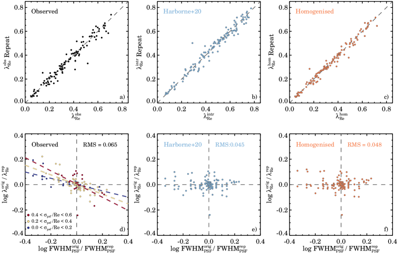
A.3 Empirical correction to account for atmospheric seeing
In this section, we test an alternative method to correct for the impact of seeing on our kinematic data. The idea here will be to use an empirical relation derived from the repeat observations to homogenise the sample to a common average seeing. Such a data driven approach has the advantage that it is not biased to the choice of simulations to derive the analytic seeing correction. For example, the analytic correction has not been designed for galaxies with complex dynamics (although the correction works relatively well with little scatter and the absolute correction for these galaxies is small). An empirical seeing homogenisation can be applied to the whole sample because it is based on the exact same observational setup and data quality as the sample that it will be applied to. The large range in morphology, stellar mass, and values for the repeat observations also remove any morphological bias. A homogenised sample might also be more appropriate to use for comparing to simulations. The philosophy here is that it is more reliable to convolve mock-observations from simulations to the seeing of an observational survey then it is to deconvolve observational results.
For these reasons, we will now derive an empirical seeing correction or homogenisation, and test how well it removes the scatter in and using repeat observations. Figs 13(a) and (d) show the results from the repeat observations without applying any corrections. We find that there is a linear trend between FWHM and , such that with a larger difference in seeing between the original and repeat, the larger the difference in . By fitting a linear relation to our data from Fig. 13(d), our goal is to remove the trend between FWHM and . Motivated by the results from the analytic correction we separate the sample into different bins of where the impact of seeing will be different. We find that:
| (18) |
| (19) |
| (20) |
The best-fit relation are shown in Fig. 13(b). As expected, with increasing fractions of the slope of the relation between and FWHM also increases. The analysis is repeated on the measurements (not shown here), from which we find the following relations:
| (21) |
| (22) |
| (23) |
We use Eq. A.3 to homogenise our measurements to a single seeing value of 20, which are shown in Fig. 13c,f. The difference between the original and repeat observations has become smaller, with a clear reduction in the RMS scatter. The method works surprisingly well given the low number of free parameters in the fit. Even more so, if we use a single relation to fit all data between , the RMS scatter only increases marginally to 0.048. In summary, homogenising the data reduces the scatter similarly as the analytic correction from Harborne et al. (2020a). In this paper, we adopt the analytic corrected to derive the intrinsic such that we can compare to previous surveys where seeing was not a limitation. However, for a comparison to mock observations from large cosmological simulations, which might be impacted by numerical resolution effects, a seeing homogenisation method might be more suitable.
Appendix B Fast and Slow rotators in ATLAS3D
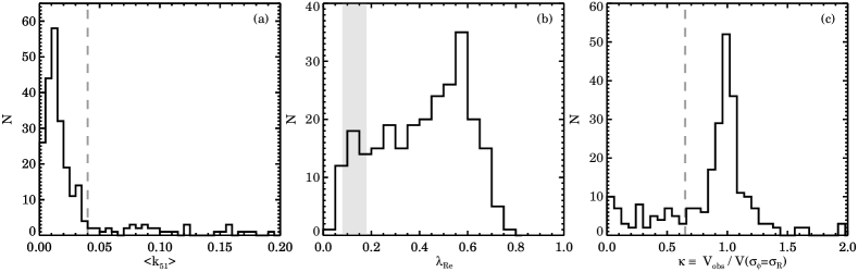
One of the goals of this paper is to investigate whether or not we can identify multiple kinematic populations in data where impact of seeing and data quality cannot be ignored. We present a framework to quantify how well kinematic identifiers are separated in the - diagram based upon the ratio of the True Positive Rate and the True Negative Rate. Here, we re-analyse results from the ATLAS3D survey, using data as presented by Emsellem et al. (2004), Cappellari et al. (2011), Krajnović et al. (2011), Emsellem et al. (2011), and Cappellari et al. (2013a, b), adapted to definitions used in this paper. For more details on these measurements we refer to van de Sande et al. (2019).
In Fig. 14 we first present the distributions of , and (see Section 5.3) which is the ratio of the observed velocity and the modelled velocity from JAM models. Note that for the values, we did not imply a JAM quality cut, as non-regular rotators are not expected to be well described by JAM models. The vertical grey lines in Fig. 14 show the commonly used selection regions for each parameter. However, we do not find clear evidence for a bimodal distribution from these three parameters, although this does not exclude the existence of a bimodality. Instead, it shows that a larger sample of galaxies is required to detect a multimodal distribution if these parameters are used independently.
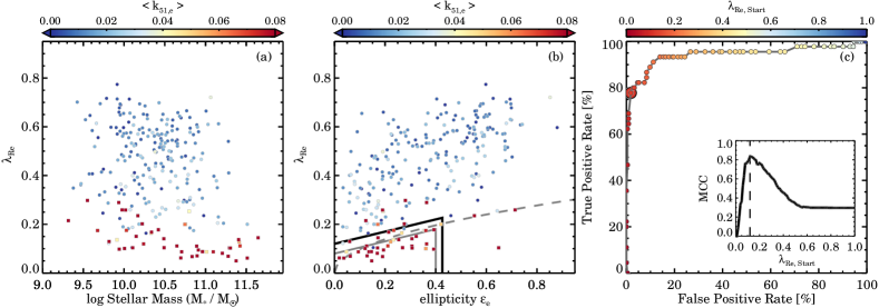
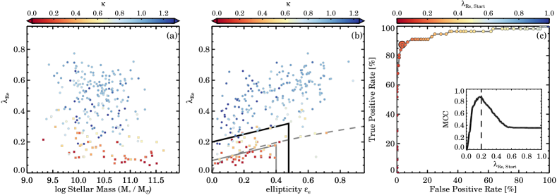
B.1 Regular and non-regular rotators from kinemetry using ATLAS3D data
Following Krajnović et al. (2011) we use kinemetry to mark the condition a galaxy can have, using to select fast rotators. We present the measurements in Fig. 15. Similar to SAMI data, we find that galaxies with high also have higher values of towards low stellar mass. When using the ROC analysis with the confusing matrix from Table 1, we find that the optimal selection region that starts at only has a True Positive Rate of 77.8 percent with a False Positive Rate of 1.9 percent. However, the Positive Prediction Value for ATLAS3D data is significantly higher than for SAMI data, with respectively 89.7 versus 70.6 percent, with a similar result for the MCC with ATLAS3D=0.83 and SAMI=0.66. The TPR for the Emsellem et al. (2011) and Cappellari (2016) selection criteria are similar but relatively low at 62.2 percent. The MCC values are 0.747 and 0.757, respectively. Thus, from a statistical point of view, we do not find a significant difference between the selection criteria from Emsellem et al. (2011) and Cappellari (2016), but we note that for example the criteria was introduced to exclude counter-rotating disks from the SR class.
B.2 Fast and Slow rotators from JAM modelling using ATLAS3D data
We will now use the parameter to classify galaxies as SR () and FR (). We use the JAM model parameters from Cappellari et al. (2013b), without applying a quality cut or limit on the inclination, but we note that with "" or inclination the results are qualitatively the same. The data and the ROC analysis are presented in Fig. 16. Similar to kinemetry, we find that galaxies with low also have higher values of towards low stellar mass. The optimal selection region is now considerably higher than the selection box from Cappellari (2016), with a starting value of and a TPR = 87.5, an FPR = 3.5, a PPV = 87.5, and an MCC = 0.875. In contrast, the TPR for the Emsellem et al. (2011) and Cappellari (2016) selection regions are both 51.8 with MCC = 0.674 and 0.682, respectively.
While the parameter presents the cleanest separation within the - diagram of all identifiers that we have used, the optimal selection is significantly higher as compared to the kinemetry optimal selection box. However, a closer look at the MCC distribution in Fig. 16(c) reveals that the peak of the MCC values is quite broad, and the relatively small ATLAS3D sample size could offset the starting value to higher values. Nevertheless, the fact the kinemetry and selection boxes differ quite considerably should be a warning that even with high-quality IFS data, the question of how to select fast and slow rotators from the - diagram is sensitive to the kinematic identifier used.
Appendix C The impact of inclination on the distributions
To test the impact of inclination on the distributions, we will compare our default measurement to values corrected to an edge-on projection. These edge-on estimates are derived from the observed and measurements following the method described in van de Sande et al. (2018). The method combines the observed properties with theoretical predictions from the tensor Virial theorem (Binney, 2005) and builds on the assumption that galaxies are simple rotating oblate axisymmetric spheroids with varying intrinsic shape and mild anisotropy (Cappellari et al., 2007). As this is an oversimplification of the known complexities of galaxy structure and dynamics, in particular for massive early-type galaxies, we therefore only use late-type galaxies for the analysis here.
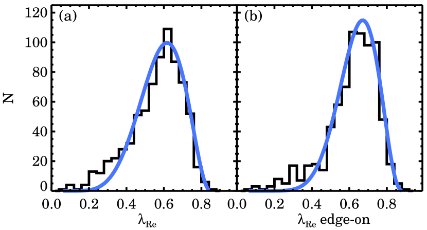
We present the and distributions for SAMI late-type galaxies in Fig. 17. The low- galaxies that are not well-fitted by the Beta function, do not disappear after applying our inclination correction. As many of these galaxies are observed close to face-on, uncertainties on the ellipticity measurements play an increasingly negative role on the inclination correction. Moreover, morphological features such as bars and spiral arms can make the galaxies’ ellipticity to appear flatter than they really are, inhibiting an accurate deprojection. Alternative methods to determine edge-on measurements will be explored in future work.
Nonetheless, the edge-on projected distribution becomes only mildly narrower () and shifts slightly towards higher from 0.586 to 0.641. As these changes are relatively small, we do not expect our results on separating a bimodal distribution to change significantly due to the effects of inclination.
Appendix D The Bayesian Mixture Model in detail
D.1 Model description
For each galaxy in our sample, we have measurements of its stellar mass () and a proxy for the spin parameter measured within one effective radius (). We aim to model a galaxy’s spin parameter, which we label to keep with standard notation in the literature, in terms of its stellar mass. We do this by building a probabilistic mixture model. In this appendix, we describe the Bayesian Mixture model used in Section 3.4 in detail.
A mixture model uses a number (in this case two) of different probability distributions to model a set of observed data. The probability of a single data point being drawn from one distribution is denoted . This implies that the likelihood function is of the form:
| (24) |
where and refer to the different probability distributions and is a vector of model parameters.
In this case, we assign and to be two distinct beta distributions, each with shape parameters and (i.e., and ). We allow these shape parameters to vary as a function of stellar mass via a first order polynomial:
| (25) | ||||
| (26) | ||||
| (27) |
These correspond to eight free parameters. Note that the beta distribution’s shape parameters must be constrained to be positive, and as such we vary them on the logarithmic scale, such that and are always greater than zero.
Furthermore, we allow the mixture probability, , to vary with stellar mass. This represents the well-known dependence of kinematic morphology with stellar mass, with massive galaxies much more likely to be slow rotators (e.g., Emsellem et al., 2011; Brough et al., 2017; Veale et al., 2017; van de Sande et al., 2017a; Green et al., 2018; Graham et al., 2018). Since is a probability, it must lie between 0 and 1. To ensure this is always the case, we use the sigmoid function to map any real number to the interval [0, 1], which also introduces a further two parameters to the model ( and ):
| (28) |
To summarise, our model has 10 free parameters; eight corresponding to the change in beta distribution shape parameters with stellar mass and two corresponding to how the probability of being drawn from either beta distribution varies with stellar mass. The final likelihood function is therefore:
| (29) |
D.2 Priors
| SAMI Observations | EAGLE | HorizonAGN | Magneticum | |||||
|---|---|---|---|---|---|---|---|---|
| Parameter | Location | Scale | Location | Scale | Location | Scale | Location | Scale |
| 0.5 | 0.3 | 0 | 3 | 1 | ||||
| 0 | 0.5 | 0 | 0.5 | 0 | 3 | 0 | 3 | |
| 0.5 | 0.3 | 3 | 1 | |||||
| 0 | 0.5 | 0 | 0.5 | 3 | 0 | 3 | ||
| 0.5 | 1 | 3 | 1 | |||||
| 0 | 0.5 | 0 | 0.5 | 0 | 3 | 0 | 3 | |
| 0.5 | 0.3 | 0.5 | 1 | |||||
| 0 | 0.5 | 0 | 0.5 | 0 | 3 | 0 | 3 | |
| 0 | 1 | 1 | 0.3 | 0 | 1 | 0 | 1 | |
| 0 | 2 | -1 | 0.3 | 0 | 2 | 0 | 2 | |
As with any Bayesian analysis, each free parameter must be assigned a prior. Our prior choices are described in Table 4. We conduct simulations to see the effect of our prior choices (known as “prior predictive checks") and ensure that our prior choices do not give rise to unphysical distributions of simulated data. Reasonable changes to these priors do not change our conclusions.