JWST/MIRI Simulated Imaging: Insights into Obscured Star-Formation and AGN for Distant Galaxies in Deep Surveys
Abstract
The JWST MIRI instrument will revolutionize extragalactic astronomy with unprecedented sensitivity and angular resolution in mid-IR. Here, we assess the potential of MIRI photometry to constrain galaxy properties in the Cosmic Evolution Early Release Science (CEERS) survey. We derive estimated MIRI fluxes from the spectral energy distributions (SEDs) of real sources that fall in a planned MIRI pointing. We also obtain MIRI fluxes for hypothetical AGN-galaxy mixed models varying the AGN fractional contribution to the total IR luminosity (). Based on these model fluxes, we simulate CEERS imaging (3.6-hour exposure) in 6 bands from F770W to F2100W using mirisim, and reduce these data using jwst pipeline. We perform PSF-matched photometry with tphot, and fit the source SEDs with x-cigale, simultaneously modeling photometric redshift and other physical properties. Adding the MIRI data, the accuracy of both redshift and is generally improved by factors of for all sources at . Notably, for pure-galaxy inputs (), the accuracy of is improved by times thanks to MIRI. The simulated CEERS MIRI data are slightly more sensitive to AGN detections than the deepest X-ray survey, based on the empirical - relation. Like X-ray observations, MIRI can also be used to constrain the AGN accretion power (accuracy dex). Our work demonstrates that MIRI will be able to place strong constraints on the mid-IR luminosities from star formation and AGN, and thereby facilitate studies of the galaxy/AGN co-evolution.
1 Introduction
Mid-infrared (mid-IR) wavelengths provide extremely valuable information for extragalactic sources. Galaxies often contain a large amount of polycyclic aromatic hydrocarbon (PAH) molecules (see Tielens 2008 for a review). When heated by starlight, these PAH molecules produce strong emission features mainly at m. In star-forming galaxies, PAHs can emit as much as of the total IR luminosity and the m PAH feature can contribute as much as 50% of the total PAH emission (e.g., Shipley et al., 2016). The PAH emission features not only can reveal important information about, e.g., metallicity and ionization parameter (e.g., Draine & Li, 2007; Shivaei et al., 2017), but also are potential redshift indicators for high-redshift objects (e.g., Chary et al., 2007).
Active galactic nuclei (AGNs) are often surrounded by large amounts of dust (e.g., Antonucci, 1993; Urry & Padovani, 1995; Netzer, 2015). The dust absorbs UV/optical radiation from the central engine and reaches temperatures of above a few hundred kelvin, much higher than the typical temperatures of interstellar dust heated by starlight (a few ten kelvin). This AGN-heated hot dust reemits the absorbed energy mainly at mid-IR wavelengths. Therefore, AGNs can be identified based on the hot dust emission (e.g., Stern et al., 2012; Assef et al., 2013; Kirkpatrick et al., 2015). The mid-IR selection of AGNs has significant advantages over other methods in terms of dust obscuration (e.g., Hickox & Alexander 2018; Alberts et al. 2020). The UV/optical selection is often affected by dust obscuration and biased to bright type 1 AGNs. X-ray data are currently the most robust method of AGN selection (e.g., Brandt & Alexander, 2015; Xue, 2017). Deep X-ray surveys can sample low-luminosity AGNs below erg s-1 up to (Xue et al., 2016; Luo et al., 2017; Vito et al., 2018). At such a low level, most () of the X-ray selected AGNs are type 2, which are potentially missed by UV/optical selections (e.g., Merloni et al., 2014). However, X-ray selection could miss a large population of extremely obscured “Compton-thick” AGNs (neutral-hydrogen column density, cm-2; e.g., Brandt & Alexander 2015; Hickox & Alexander 2018). These obscured AGN can be identified through warm-dust emission from the AGN in the mid-IR (e.g., Alexander et al., 2008; Del Moro et al., 2016), and therefore it is useful to explore the utility of mid-IR observations to identify these objects.
Past and current facilities have not been sufficiently sensitive to capture the mid-IR fluxes from most sources in the distant universe. Until now, the most sensitive mid-IR facility has been Spitzer/IRACMIPS, covering wavelengths 3.6–24 µm. However, the IRAC+MIPS coverage has a large uncovered gap between the longest IRAC band (m) and the shortest MIPS band (m), leaving a large room for model degeneracy at mid-IR wavelengths. For example, observations have found some galaxies with elevated 24 m emission compared to that expected from star formation (mid-IR-excess galaxies; e.g., Daddi et al., 2007a; Papovich et al., 2007). The mid-IR excess emission may be interpreted as either PAH emission or AGN-heated dust radiation, and it is challenging to decompose these two components with broad-band imaging alone that lacks contiguous mid-IR wavelength coverage (e.g. Daddi et al., 2007b; Azadi et al., 2018). Furthermore, the Spitzer imaging has a large point spread function (PSF, FWHM at m), causing source-confusion issues in crowded deep fields (e.g., Dole et al., 2004; Ashby et al., 2018). AKARI/IRC provided contiguous wavelength imaging over 2–26 m. However, its sensitivity is relatively low compared to Spitzer, and many Spitzer faint sources are undetectable by AKARI (e.g., Papovich et al., 2004; Clements et al., 2011). Due to the lack of sensitive 8–24 m imaging, many of the IR AGN selection techniques are forced to use m colors that are also biased toward type 1 AGNs, similar to UV/optical selections (e.g., Donley et al. 2012; Li et al. 2020).
The upcoming James Webb Space Telescope (JWST) mission will revolutionize the field of infrared astronomy. The onboard Mid-Infrared Instrument (MIRI), equipped with both an imaging camera and a spectrograph, covers a wavelength range from to 28m. The sensitivity of MIRI is generally orders of magnitude higher than Spitzer (e.g., Glasse et al., 2015), able to capture the bulk of cosmic mid-IR emission (e.g., Bonato et al., 2017; Rieke et al., 2019). The MIRI imager has a PSF FWHM of –. The sub-arcsecond angular resolution provided by MIRI reduces greater source blending and source confusion. The detector’s field of view (FOV) is , sufficient for extragalactic surveys. MIRI has a total of 9 broad-band filters with contiguous wavelength coverage, and able to well characterize the mid-IR spectral shape.
Aside from observational facilities, reliable techniques are also essential for the estimation of source properties. Past methods have relied on color-selection (and color-color selection) to classify IR sources (e.g., Stern et al., 2005; Donley et al., 2012; Messias et al., 2012; Kirkpatrick et al., 2017). The color-color methods provide a mechanism to classify galaxies as AGN versus non-AGN, and to identify candidates for “composite sources” (e.g,. Kirkpatrick et al., 2017). These methods can be be straightforwardly applied to a large sample of sources. Indeed, previous work has shown that MIRI mid-IR color-color diagrams can reliably identify AGNs in galaxies down to low AGN luminosities (Eddington ratios of , e.g., Kirkpatrick et al. 2017). However, color-color methods have disadvantages. They often require knowledge of the redshift of the source a priori to interpret (for example, the redshift can determine which colors best separate warm dust heated by AGN from emission from PAHs). In addition they are typically binary (either a source is an AGN or it is not), or trinary (including composite sources). Lastly, typical color-selection methods use only a portion of the available information (e.g., a color-color diagram only uses flux densities measured at passbands). Historically, these methods have been very successful. However, as the amount of available data and passbands increases (as will be the case in the JWST/MIRI era) it is prudent to explore methods that can provide more detailed constraints using the full dataset, and thereby improve our understanding of the co-evolution of AGN and star formation in distant galaxies.
An alternative type of quantitative method to characterize the IR emission from sources is spectral energy distribution (SED) fitting. SED fitting has been successfully applied to AGN identification/characterization in previous works, based on the fact that AGNs and star-forming galaxies typically have distinctive SED shapes (e.g., Alonso-Herrero et al., 2006; Caputi, 2013; Chang et al., 2017). SED-fitting methods typically fit the photometric data with numerous model templates. They are more computationally intensive than color-color methods, but they have the advantage that they can simultaneously take into account all photometric data, and fit for multiple model parameters, including fitting for a photometric redshift (e.g., Małek et al., 2014). Simulations indicate that MIRI data, when included in the SED fitting, can significantly improve the accuracies of fitting results (e.g., Bisigello et al., 2016, 2017; Kauffmann et al., 2020).
Here, we employ one such SED-fitting method, x-cigale, which is an efficient python code that can model multiwavelength galaxy/AGN SEDs from X-ray to radio (Yang et al., 2020). Compared to its original version, cigale (Boquien et al., 2019), x-cigale implements many AGN-related improvements. For example, x-cigale allows a polar-dust component that has been recently observed with high-resolution imaging of local AGNs (e.g., Asmus, 2019; Stalevski et al., 2019). Thanks to its optimized parallel algorithm, x-cigale is able to fit thousands of SEDs using millions of models within a few hours on a typical multi-core desktop/laptop. x-cigale adopts physical models following the law of energy conservation. Aside from the traditional least- analysis, x-cigale also allows simultaneous analysis for source properties such as redshift and (where is the fraction of total dust IR luminosity attributed to the AGN) in a Bayesian style. The Bayesian analysis considers the full probably density functions (PDFs). In contrast, the least- analysis only considers the best-fit SED model and the non-negligible probability of other models may be neglected. Therefore, the Bayesian results provide estimates of the PDFs for model parameters that are more informative than minimum- results (e.g., Pirzkal et al., 2012; Boquien et al., 2019).
In this paper, we investigate the potential ability of deep imaging with JWST/MIRI to constrain the properties of distant galaxies. We use as our fiducial example the MIRI observations expected as part of the Cosmic Evolution Early Release Science (CEERS) survey, including the existing multiwavelength photometry expected with that dataset. We simulate a realistic set of galaxy flux densities in the MIRI bands, using predictions from real galaxies observed in deep HST imaging from CANDELS (Grogin et al., 2011; Koekemoer et al., 2011; Stefanon et al., 2017). We then generate simulated raw MIRI images that account for realistic estimates of the noise. We then reduce MIRI raw imaging data to obtain MIRI mosaics that are matched to the existing HST/CANDELS imaging. We measure the mid-IR fluxes in the MIRI bands. We then perform SED fitting with x-cigale on the fluxes of MIRI and currently existing bands in UV-to-IR wavelengths. The redshift and other source properties are fit simultaneously in this SED-fitting process, where results are then derived by marginalizing over the other parameters. Finally, we evaluate the results by comparing the SED-fitting source properties with the model input ones.
This paper is structured as follows. In §2, we describe the CEERS survey, the existing CANDELS catalog, the construction of our model MIRI flux densities, and how we generated the simulated MIRI (raw) data. In §3, we discuss the reduction of the simulated MIRI raw data, method for measuring matched-aperture flux densities, and we analyze the SEDs (using SED fitting from x-cigale). We then assess the results, focusing on the ability to constrain the photometric redshifts and of distant galaxies by including the MIRI data. In §4, we discuss our results and future prospects using JWST/MIRI for this application. We summarize our work in §5.
Throughout this paper, we assume the same cosmology as x-cigale, i.e., a flat CDM cosmology with km s-1 Mpc-1 and (WMAP7; Komatsu et al. 2011). We adopt a Chabrier initial mass function (IMF; Chabrier 2003) for relevant quantities (stellar masses, etc.). Quoted uncertainties are at the (68%) confidence level. All magnitudes are in AB units (Oke & Gunn, 1983), where for in units of erg s-1 cm-2 Hz-1.
2 Sample and data
2.1 The CEERS survey
The Cosmic Evolution Early Release Science (CEERS) Survey is an approved JWST program (Finkelstein et al., 2017), covering arcmin2 in the Extended Groth Strip field (EGS). CEERS consists of 63 hours of NIRCam (1–5 m) and MIRI (5–21 m) imaging, NIRSpec and spectroscopy, and NIRCam/grism spectroscopy. CEERS will be one of the first public JWST surveys with data publicly available 5 months after acquisition in Cycle 1.
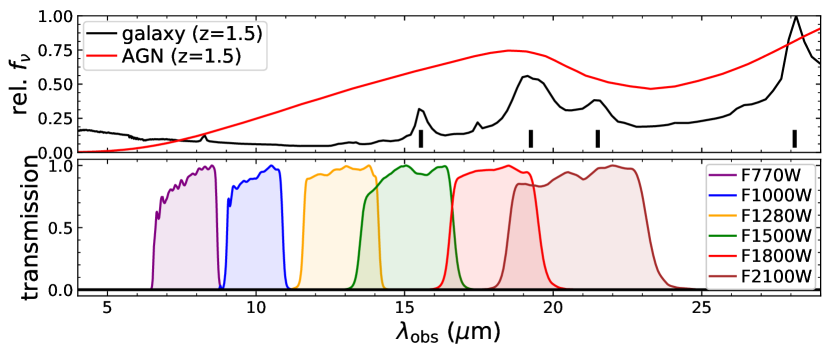
CEERS has four MIRI pointings, labeled as MIRI 1–4 fields, respectively. In this paper, we focus on the MIRI2 pointing that has the widest wavelength coverage of six bands: F770W, F1000W, F1280W, F1500W, F1800W, and F2100W. MIRI2 is centered at (, ).111The coordinate is based on a spring launch configuration, which might differ from the future true pointing. However, the sample in this work is broadly representative of an arbitrary extragalactic pointing, and the conclusions should not depend on the exact pointing coordinates. For the five bands from F770W to F1800W, the planned exposure time is 1665 seconds/band (3 dithers/band); for F2100W, the exposure time is 4662 seconds (6 dithers). The designed limiting magnitudes in the proposal are 25.5 (F770W), 24.8 (F1000W), 24.3 (F1280W), 23.8 (F1500W), 22.9 (F1800W), and 22.8 (F2100W). Fig. 1 displays the transmission curves of the available MIRI bands in the MIRI2 pointing.
With the goal of making our simulation as realistic as possible, we use all available data for the galaxies in the CEERS/MIRI2 field. Our work is based on the F160W (-band) selected CANDELS/EGS catalog (Stefanon et al., 2017). In this catalog, there are 463 sources down to within the MIRI2 pointing. Only 8 of these sources have secure spectroscopic redshift (spec-) measurements, while the rest have photometric redshifts (photo-) from Stefanon et al. (2017). These CANDELS/EGS sources are mostly in the redshift range of –3. The CEERS/MIRI2 region is covered by 15 broad bands from CFHT/MegaCam to Spitzer/MIPS 24 m (Dickinson et al., 2006; Stefanon et al., 2017). Although this region is also covered by Herschel (Lutz et al., 2011; Oliver et al., 2012), most of our sources are beyond the sensitivity of Herschel (only two sources in the current MIRI2 field are detected () by PACS and none by SPIRE). Therefore, we do not use Herschel data in this work due to the low detection rate. Based on these photometric and redshift data, we obtain the model input MIRI fluxes in §2.2.
2.2 The model MIRI fluxes
We have incomplete knowledge as to which galaxies in the CANDELS catalog (within MIRI2 pointing) host AGNs, because the currently existing photometric data provide very weak constraints on AGN emission (see §3.3.2). However, considering the relatively small area of MIRI FOV (2.2 arcmin2), we estimate that only AGNs (out of 463 sources; §2.1) actually exist within the MIRI2 pointing, based on the AGN number density derived from the deepest X-ray survey, 7 Ms Chandra Deep Field-South (CDF-S; Luo et al., 2017). Actually, none of the MIRI2 galaxies have been detected by the existing 800 ks X-ray data in the EGS field (2–7 keV; Nandra et al. 2015). Therefore, in §2.2.1, we first model the SEDs of real existing photometry with pure galaxy models (i.e., ), and integrate the best-fit SEDs with the MIRI filter transmission curves to obtain the bandpass-averaged flux densities as inputs to the MIRI simulations. To test the cases when AGN is present, we also add a hypothetical AGN component to the best-fit galaxy SEDs and rederive the MIRI flux densities to test for this possibility in additional sets of simulations in §2.2.2. These MIRI fluxes are used as the model input in our simulations of MIRI imaging data §2.3.
2.2.1 Pure galaxy models based on empirical SEDs
We obtain model MIRI fluxes based on the SED fitting of real observations. We fit the currently existing broad-band photometric data (from Stefanon et al. 2017) that exist for the galaxies in the nominal MIRI2 pointing (§2.1) with x-cigale (Boquien et al., 2019; Yang et al., 2020). We do not use the X-ray module of x-cigale due to the lack of X-ray detections (§2.2). In the x-cigale analysis, we fix the redshift at the spec- value (when available) or otherwise the photo- from the CANDELS/EGS catalog (Stefanon et al., 2017). The fitting parameters are similar to those used by Yang et al. (2020) and are summarized in Table 1. As in Table 1, we adopt the model of Dale et al. (2014) for galactic dust emission. In this model, a single parameter of radiation slope222, where and represent dust mass and radiation strength, respectively. controls the IR SED shape (e.g., the MIR/FIR ratio and PAH emission strength). The model is derived from observations of local galaxies, and admittedly it may deviate from the true IR SEDs of distant sources. However, for this exercise it is sufficient as our goal is to recover the mid-IR emission. In the future, new models dedicated for distant galaxies can be obtained using empirical measurements from the MIRI data themselves (especially if additional spectroscopy from the medium-resolution spectrometer, MRS, becomes available). We will implement these new models to x-cigale to facilitate the modeling of distant galaxies with real MIRI data.
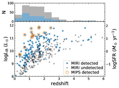
After running x-cigale, we obtain the model MIRI fluxes by integrating the best-fit SEDs with the transmission curves of MIRI filters (Fig. 1). Fig. 2 shows the best-fit dust IR luminosity as a function of redshift. Because we do not have FIR data to directly constrain galaxy cold-dust emission, the IR luminosity largely comes from the modelling of UV/optical stellar extinction, but this is satisfactory for our purposes here where we study the measured mid-IR emission from MIRI based on the simulations. x-cigale follows energy conservation, and thus the extincted UV/optical luminosity equals the dust re-emitted IR luminosity.
| Module | Parameter | Values |
| Star formation history | (Gyr) | 0.1, 0.5, 1, 5 |
| (Gyr) | 0.5, 1, 3, 5, 7 | |
| Simple stellar population Bruzual & Charlot (2003) | IMF | Chabrier (2003) |
| Stellar extinction Calzetti et al. (2000) Leitherer et al. (2002) | 0.1, 0.2, 0.3, 0.4, 0.5, 0.7, 0.9 | |
| Galactic dust emission Dale et al. (2014) | Radiation | 1.0, 1.5, 2.0, 2.5 |
| slope | ||
| Redshifting | Fixed at of | |
| Stefanon et al. (2017) |
Note. — For parameters not listed here, we use x-cigale default values.
2.2.2 Hypothetical AGN-galaxy mixed models
In §2.2.1, we derive the model-input MIRI fluxes from pure-galaxy templates based on the real existing photometry. Now, we add a hypothetical AGN component to the SEDs to explore the cases when an AGN is present. The purpose of using realistic galaxy templates is to test, if a galaxy in our field hosts an AGN, how well we can detect/characterize the AGN component. As we argue below (§ 4.2) MIRI observations may be sensitive to the presence of emission from obscured AGN even in galaxies that are not detected in the X-ray data. For this reason, it is useful to test the ability to recover the AGN emission in these “real” objects like those that will be seen in CEERS.
To generate AGN-galaxy mixed SEDs, we again employ x-cigale, which not only fit the photometric data but also generate model SEDs with given physical parameters. For each source, we adopt the best-fit parameters in §2.2.1 for the galaxy component. Then, we add an AGN component with the SKIRTOR model in x-cigale (Stalevski et al., 2012, 2016). SKIRTOR is a modern clumpy torus model based on Monte Carlo simulations. Yang et al. (2020) introduced a polar-dust component to this model when implementing it to x-cigale.
For the AGN model parameters, we set the torus angle (between horizontal plane and torus edge) as 40∘ (the x-cigale default value), which is favored by the observations of Stalevski et al. (2016). We randomly choose a viewing angle (between AGN axis and line of sight) among 60∘, 70∘, 80∘, and 90∘. We do not include smaller face-on viewing angles that correspond to type 1 (broad-line) AGNs. These AGNs are typically luminous as the UV/optical emission from the central engine is directly visible. Therefore, their properties such as redshift and AGN luminosity can be well measured with UV/optical spectroscopy and photometry. Also, most AGNs selected in deep X-ray surveys are type 2 (see §1). In this paper, we focus on type 2 AGNs for which the UV/optical emission is entirely obscured and therefore our choice of the larger viewing angles is appropriate.
For other AGN torus parameters such as the 9.7 m optical depth () and radial profile index (density ), we randomly assign values to each source from all allowed values in the SKIRTOR model (e.g., and ). For the AGN polar-dust , temperature, and emissivity, we randomly assign values for each source from ranges of 0–0.3 (SMC extinction law), 100–300 K, and 1–2. This random choice of model parameters is to represent the diversity of torus physical properties based on current constraints (Stalevski et al., 2012, 2016). There are a total of nine parameters describing the hypothetical AGN component. We note that four of these parameters are free when we perform the SED fitting while the other five parameters are fixed to canonical values (see §3.3). We further note that the values of these fixed parameters do not impact the conclusions here (see also Yang et al., 2019).
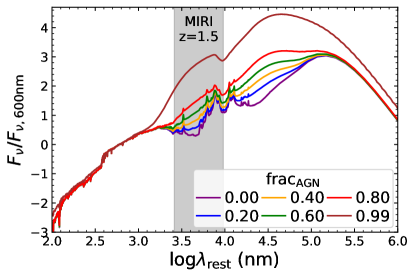
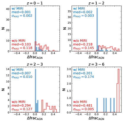
After determining the AGN parameters above, we generate the total (galaxy AGN) SEDs with a given , and convolve the SEDs with MIRI filter curves to obtain model-input MIRI fluxes. We adopt five values of 0.2, 0.4, 0.6, 0.8, and 0.99, for different AGN strengths.333The pure-galaxy models in §2.2.1 can be considered as . For each , we perform a set of MIRI simulations in §2.3. Fig. 3 shows a set of SED models with different values (as a reminder, is the fraction of the IR luminosity [3–1000 µm] from the AGN component). As increases, the shape of mid-IR SEDs changes significantly, because AGN hot-dust emission mostly concentrates on mid-IR wavelengths. After inserting the hypothetical AGN component, the flux densities at other bands may exceed the observed fluxes (this is especially for the IRAC and MIPS bands), and we deal with this issue in §3.3 by generating mock fluxes for these bands from the new SED.
2.3 The simulations of imaging data
We use mirisim (version 2.2.0; Klaassen et al. 2020) to simulate the images of MIRI bands. mirisim, developed by the MIRI European Consortium, is a dedicated simulation package for the JWST/MIRI instrument. mirisim accepts source positions, fluxes, and morphological shapes as input. The MIRI images generated by mirisim are preliminary (raw) “level 0” data products, and need to be processed through the jwst calibration pipeline444https://github.com/spacetelescope/jwst (pipeline hereafter) for further reduction (§3.1). In this way, mirisim provides data products equivalent in format to what we expect JWST to deliver.
We set the background noise as “low” in mirisim, as the EGS region has weak zodiacal background (Finkelstein et al., 2017). We set the background spatial gradient to 5%/arcmin (i.e., the background changes by 5% per arcmin) with a position angle (PA) of . We adopt a dither pattern identical to the one in the CEERS Astronomer’s Proposal Tool (APT) file, optimized for parallel observations between Near Infrared Camera (NIRCam) and MIRI (Finkelstein et al., 2017). The exposure duration for each dither is the same as that in the CEERS APT configuration (using the same Groups/integration, integrations/exposure, and exposures/dither as expected for CEERS; §2.1). The detector readout mode is set to “fast”, the same as proposed for CEERS. The input fluxes are the model fluxes obtained in §2.2.
Besides a point-like source profile, mirisim also allows galaxy morphologies with Sérsic profiles. Based on the HST F160W imaging data, van der Wel et al. (2012) performed Sérsic fitting (Sersic, 1968) for galaxies in the CANDELS/EGS field. We adopt their results for sources with good fitting quality (flag ). For the rest of the sources (flag or ), we adopt a point-like profile as mirisim input to test results for unresolved sources. The adopted galaxy profiles have diameters () of – (20%–80% percentile), while the MIRI PSFs have FWHMs ranging from (F770W) to (F2100W). Therefore, MIRI can spatially resolve a non-negligible fraction of the CANDELS galaxies even at m. In this work, we assume that the AGN and galaxy emissions have the same morphology, but in reality the former is likely more compact than the latter. Therefore, a source could be more compact in MIRI than in F160W due to the presence of an AGN. Such a morphological difference between MIRI and F160W could serve as an AGN indicator. We leave the investigation of this potential technique of AGN identification to future works.
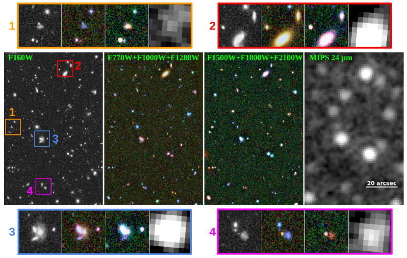
For each model-input (§2.2), we perform an independent set of mirisim simulations for all the six MIRI bands (from F770W to F2100W). Fig. 4 displays the simulated images of the pure-galaxy case in false (RGB) color (after the data reduction in §3.1). It is clear that the colors and morphologies from MIRI will provide an unprecedented view of the IR emission from distant galaxies compared to previous missions (e.g., MIPS 24 µm).
Since our simulations are based on the CANDELS F160W sources, we assume that all MIRI sources are detected in F160W. We acknowledge that a new type of optically-faint MIR-bright sources could actually exist, and such sources may be detectable by MIRI but not by F160W. The real MIRI images after launch will provide a great chance to explore this unknown regime of distant galaxies.
In addition to the real CANDELS sources, we also simulated a set of bright point sources in Appendix A using the CEERS MIRI exposure configuration. These point sources are used for the purposes of data validation, photometric tests, and corrections (see Appendix A). For the photometry extraction purpose (see §3.2.1 for details), we also need to simulate HST F160W images using the identical galaxy morphologies (i.e., pure Sérsic models) that are equivalent to those in the simulated MIRI images. We describe the simulated F160W images in Appendix B.
3 Data processing and analyses
3.1 The reduction of MIRI imaging data
We run the JWST pipeline (version 0.15.2) to process the mirisim output of the level 0 data from mirisim (§2.3). The level 0 data for each dither is in the format of a FITS file. There are three stages of data processing. Stage 1 performs detector-level corrections for individual dithers, producing count-rate maps from the “up-the-ramp” readouts. Stage 2 applies physical corrections and calibrations to individual dithers, producing flux maps with image header containing standard World Coordinate System (WCS) information. Stage 3 combines individual dithers to a single image.
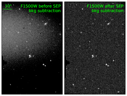
Stage 1 involves the rejection of cosmic rays, which are deposited onto the imaging data during the exposure. While this process successfully rejects most () of the cosmic rays, it still misses up to cosmic rays per dither after visual inspection. To clean up these outliers, we run astro-scrappy555https://github.com/astropy/astroscrappy which implements the “Laplacian Edge” algorithm of cosmic-ray detection (see van Dokkum 2001), and mask the pixels polluted by the detected cosmic rays. Stage 3 involves background subtraction before merging the dithers. However, the current version of pipeline only subtracts a single global background value, although the actual background may have spatial dependence due to instrumental thermal emission and/or scattered light. Therefore, before merging the dithers, we perform an additional background subtraction with sep (version 1.0.3; Barbary 2016), which realizes the core algorithms of source extractor (Bertin & Arnouts, 1996) in python. We adopt a cell size of 32 pixels (pixel size ) and a median-filtering size of 3 cells. Fig. 5 demonstrates the effect of our background subtraction. After this background subtraction, we find there is a small fraction of pixels () that have extremely negative values ( uncertainties) in the F1800W and F2100W images. The status of these pixels are not marked as abnormal in the associated quality map. Therefore, we manually mask these pixels by setting their values to zero and their status as abnormal.
Stage 3 provides the a final image that merges all the individual images for that band. We find the merged images also show traces of a residual background, especially for the red bands (F1800W and F2100W) where the background is stronger. Therefore, we repeat the background subtraction step again with the same sep parameters as above. This process effectively removes the residual background for each band. The merged images have a native pixel size of . We find that the background-subtraction procedure above does not bias the measured flux densities (see Appendix A), so we conclude this background is mostly additive and removable by this procedure.
However, for photometry we make an additional set of MIRI mosaics at the pixel scale of the HST F160W image. The simulated HST F160W image has a pixel size of . Our process of photometry extraction (§3.2) requires that MIRI and F160W images have pixel scales that are integer multiples of this pixel scale. Because the current version of pipeline does not allow a user-defined pixel size for the final image, we reprojected the MIRI images to the frame of the simulated F160W image for our photometric step (utilizing the reproject_exact function of astropy (Astropy Collaboration et al., 2018)). The algorithm of reproject_exact is designed to conserve fluxes, so the final image is oversampled to the F160W pixel scale (/pixel where the fluxes are conserved.
3.2 The extraction of MIRI photometry
We utilize tphot (version 2.1; Merlin et al., 2015, 2016) to measure MIRI fluxes. tphot performs PSF-matched photometric measurements based on a “template-fitting” technique (Laidler et al., 2007). First, for each source from a given “high-resolution” image, it crops a template (i.e., a cutout containing this source) and normalize the total flux to unity. tphot then convolves these templates with a given PSF kernel. This kernel matches the PSF of the high-resolution image to that of the “low-resolution” image (i.e., the image for photometric measurements). Next, tphot makes a model low-resolution image by convolving these templates with the kernel and normalizing it to have unity flux. Finally, the code scales the templates for sources near the source of interest simultaneously so that the model image is an optimal match to the values in the input low-resolution image (through minimization). The scaling factor for each template is the output best-fit flux for the corresponding source.
We opt to use “forced photometry” models (specifically tphot Merlin et al. 2015, 2016) instead of methods that measure direct aperture photometry (e.g., source extractor Bertin & Arnouts 1996) for MIRI photometry extraction, as the former (tphot) accounts for different PSF sizes in different bands without degrading the image quality and can provide flux densities measured in matched apertures for all objects detected in a catalog. It is also possible to perform PSF-matched photometry under the “dual image” mode of source extractor. However, this typically requires to degrade all images to a dataset’s largest PSF (F2100W in our case) so that all PSFs across different bands become similar (e.g., Yang et al., 2014). In our case, this approach means a huge loss for the imaging quality of the blue MIRI bands, because, e.g., the F770W PSF is times sharper than the F2100W PSF. Therefore, we consider that our tphot approach is superior to this one.
We note that it is possible to run source extractor on each MIRI image independently, and then match the detected single-band MIRI sources with the CANDELS/EGS catalog. However, another advantage to using forced-photometry methods, such as TPHOT is that they are able to measure flux densities (or upper limits) for all sources in a catalog. This provides useful constraints on the emission (in the case here on the mid-IR emission) which can place limits on the amount of warm dust from AGN or molecular emission from star-formation on all galaxies in our catalog. We present a detailed comparison between the photometry of tphot and source extractor in Appendix C. The results show tphot performs better than source extractor, justifying our choice of the former.
3.2.1 TPHOT preparation
We adopt the simulated HST F160W map (Appendix B) as the input high-resolution image and the simulated MIRI maps as the low-resolution images. We adopt this step because we expect (nearly) all galaxies detected in the red-MIRI bands to be detected in the deep CANDELS HST F160W imaging. The full width at half maximum (FWHM) of F160W PSF is , smaller than those of MIRI bands (ranging from F770W to F2100W ). As a reminder, for the test here we use the simulated F160W image (using identical morphological models as used in the MIRI simulations). The reason to use the simulated F160W image rather than the observed one is that, some sources in the observed F160W image have morphologies with structures that are not represented by the simple Sérsic profiles used to create the MIRI images. This is especially true for some large (angular-size) galaxies that show asymmetric features (tails, star-forming knots, disturbed morphologies, see Figure 23, for example). When processing the real observed MIRI images in the future, the observed F160W image rather than the simulated one should be used, as we expect the morphologies between the real F160W and actual MIRI imaging will be more consistent than the models used here.
Our tphot run also needs the kernels that transform (through convolution) the F160W PSF (Appendix B) to match the MIRI PSFs. We obtain the MIRI PSF for each band using webbpsf. webbpsf can only generate PSFs with pixel sizes of 0.11, where is a user-defined integer. We first generate a PSF with 0.055/pixel. We then re-project this PSF to the F160W PSF of 0.06/pixel using reproject_exact (Astropy Collaboration et al., 2018). Our PSFs have a format of , which is much larger than the FWHM of each PSF profile (F2100W ). We have also tested larger PSFs (e.g., ) and the resulting photometry only has limited minor changes, but the tphot run becomes significantly slower.
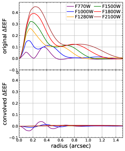
To derive the kernels, we utilize pypher (version 0.6.4; Boucaud et al. 2016) which is based on Wiener filtering. pypher has a tunable regularization parameter (). A lower value leads to higher fidelity at the expense of smoothness. The fidelity can be measured as EEF (encircled energy fraction) between the convolved high-resolution PSF (F160W) and the low-resolution PSF (MIRI bands). We normalize the total fluxes of all the input PSFs to unity before feeding them to pypher. We adopt a value of 0.03, which leads to EEF always below 4% at any radius for all of the MIRI bands (and better than 1% for all radii, except for F770W). Fig. 6 displays the EEF (before and after the convolution) as a function radius for different MIRI bands. After the convolution, EEF becomes much smaller, demonstrating the effectiveness of the kernels constructed by pypher.
tphot also needs a source list and a segmentation map for the input high-resolution image (F160W), and we run source extractor (Bertin & Arnouts, 1996) to generate these ingredients. The segmentation map describes the pixel area covered by each source, and the area is critical in affecting the tphot photometry. A small area may miss a significant fraction of light in tphot analysis, systematically leading to a lower flux. On the other hand, a large area may include too many noise-dominated pixels, increasing the uncertainty of the output flux. The segmentation map is mainly controlled by the parameters “detect_thresh” and “detect_minarea” in source extractor (Bertin & Arnouts, 1996). We find that a setting of detect_thresh and detect_minarea is appropriate in producing optimal tphot photometry (see §3.2.2), and we adopt this setting. We note that a typical configuration (i.e., higher detect_thresh and lower detect_minarea) would lead to a significant flux underestimation due to the missing of faint wings. Our source extractor run detects 545 sources. We associate these sources with the simulation input catalog (i.e., the CANDELS/EGS catalog of 463 sources; see §2.2) using a matching radius, and find 388 matches. Most of the 75 () undetected sources are faint with , and only a few of them would be MIRI-detected given their expected low MIRI fluxes (the pure-galaxy models; §3.2.2). The extra 157 () sources detected by source extractor are noise likely due to our low-detect_thresh setting. This is acceptable as our main goal is to study the recovered MIRI flux densities for the majority of the (brighter) sources detected in the F160W image. We therefore exclude the sources with no associated source in the input CANDELS/EGS catalog.
3.2.2 TPHOT results
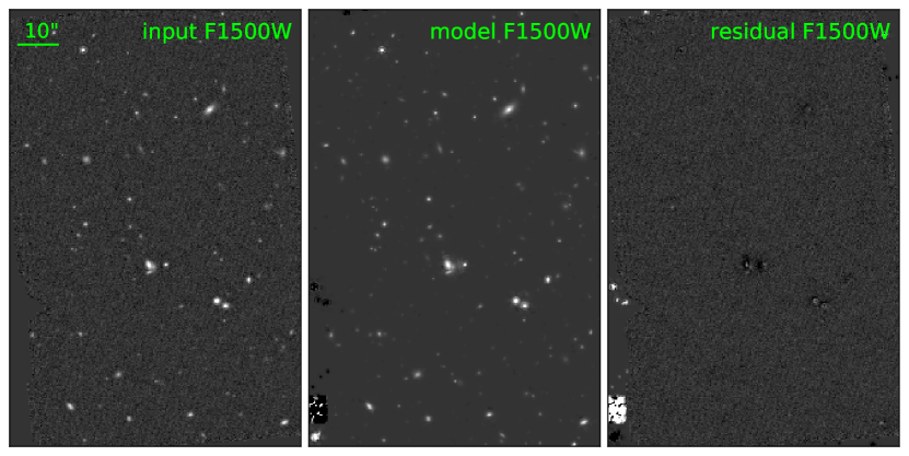
We run tphot (Merlin et al., 2015, 2016) on each MIRI band individually, while using the simulated F160W image and associated source extractor results as high-resolution prior (§3.2.1). Fig. 7 shows the input, model, and residual maps for F1500W (pure-galaxy model; §2.2.1) as an example. Overall, the model map looks very similar to the input map, and the residual map is dominated by noise (except at some spots outside of MIRI detector coverage). This result indicates that tphot successfully models the MIRI galaxy profiles with PSF matching. Some sources close to the image edges are poorly constrained due to the lack of good imaging coverage. These objects are flagged by tphot, and we exclude them from further analysis for this reason.
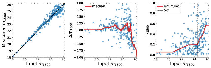
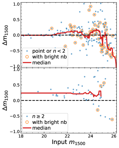
In Fig. 8, we compare the tphot-measured and input magnitudes (also for the F1500W of pure-galaxy model as an example). From Fig. 8 (middle), the measured magnitudes tend to be slightly fainter than the input magnitudes (except for the faint tail of ). The cause could be that we miss some light from the faint wing component of the source profiles. To investigate this possibility, we divide the sample by (input) Sérsic index. We re-plot Fig. 8 (middle) for Sérsic and point sources versus sources, respectively, in Fig. 9 (see Appendix D for the full version including all bands). The latter have more significant wing component than the former (see, e.g., Häussler et al. 2007). From Fig. 9, the measured magnitudes for and point sources do not suffer from significant systematics, but those for sources show a bias of up to several tenths of a magnitude. This result indicates that the light loss due to faint wings indeed causes systematic offset in photometry measurements, and care is needed to interpret the flux densities of these objects. Currently these objects constitute a minority of the sources (only 21% of the F1500W sources). As we do not know what the morphologies of MIRI sources will be, we defer more detailed analysis to a future work.
In Fig. 9, we indicate crowded sources () having at least one neighbor (within radius) brighter than mag. These are objects where flux residuals from the (relatively) bright companion can bias the flux measurements of the sources. From Fig. 9, the measured photometry of these sources is not always deviant from the distribution, although we notice that these sources do have a larger scatter (, where MAD is the median absolute deviation) in compared to isolated sources (0.23 vs. 0.17 for the sources in Fig. 9 top). The sources with neighbors only contribute to a small fraction of the population (e.g., 15% for F1500W). Therefore, we conclude that source crowding does not significantly affect the quality of our measured photometry, and it is clearly superior to previous instruments thanks to the high angular resolution of MIRI (see, e.g., Fig. 4).
The photometric errors in the tphot output are based on the fitting of low-resolution source profiles (§3.2). We find that these errors are often significantly smaller (up to a factor of ) than the actual differences between the measured and input magnitudes. This underestimation of uncertainties could be possibly due to the assumption of pixel-noise is uncorrelated in tphot (Merlin et al., 2015, 2016). We do not adopt the tphot uncertainties. Instead, we establish an empirical “error function” for each MIRI band based on the distribution of input-to-measured flux densities. First, we bin our sources on their input MIRI magnitudes with each bin containing 30 sources. For each bin, we calculate the median input magnitude and the median difference between the measured and input magnitudes. Finally, we obtain the error function by linearly interpolating the median difference as a function of median magnitudes (see Fig. 8, right). Although the error function for each band is derived based on the simulation set of pure-galaxy models (§2.2.1), we also apply it to the other simulation sets with non-zero (§2.2.2). From Fig. 8 right, the uncertainty is mag at the bright end, and rises toward faint sources as expected. For each source, we estimate the magnitude uncertainty by evaluating the error function on the measured magnitude.
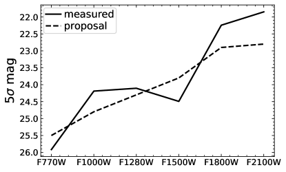
We estimate the 5 limiting magnitude for each band as the value where the error function equals 0.217 mag, corresponding to (assuming standard error propagation, ). Fig. 10 compares these measured limiting magnitudes and those expected for CEERS (Finkelstein et al., 2017) based on JWST Exposure Time Calculator (ETC), assuming a point-source profile. From Fig. 10, our measured depths are similar to those in the CEERS proposal (differences mag), where we interpret offsets as a result of limited sample sizes, our more realistic treatment of source surface brightness profiles and source crowding, and different background-noise assumptions of mirisim (spatially dependent; §2.3) versus ETC (uniform). We consider the last factor is mainly responsible for the relative large difference between the F2100W depths of mirisim and ETC (0.95 mag; Fig. 10), as the F2100W has the strongest background in our filter set. However, whether the background is spatially dependent or not can only be determined from the real MIRI imaging data after launch. For now, we caution that the ETC S/N could be over-optimistic for F2100W (and also F2550W for which background is even stronger than F2100W), because ETC does not account for the spatial dependence of background.
3.3 The SED fitting
We again use x-cigale to perform SED fitting of the galaxies’ (simulated) photometry that includes measurement errors on the photometry. To assess the effects of MIRI data, we focus the sources having significant () detections in at least two MIRI bands (Fig. 2). For the simulation set of pure-galaxy models (§2.2.1), these MIRI sources consist of 53% and 75% of the and population, respectively. For the simulation sets of AGN-galaxy models (§2.2.2), the detection rates are even higher due to the additional AGN contribution. In contrast, the MIPS m detections rates are only 5% () and 9% () in the real data. The high detection rates of MIRI highlight its superior flux sensitivity.
For the currently existing non-MIRI bands, we cannot use the actually observed photometry directly in the SED fitting. The reason is that the observed photometry is not entirely consistent with that expected from the SED models used to generate model-input MIRI fluxes (§2.2). This is especially a serious issue for the models of high . When we add a strong hypothetical AGN component to the galaxy SED (§2.2.2), the model-expected IRAC and MIPS fluxes could be significantly higher than the observed values. Another issue is that our adopted model-input redshifts are mostly photo- from the CANDELS/EGS catalog (§2.2), and these photo- are just an approximation, not the “true” values. However, to assess the accuracy of our SED-fitting results, we need the true redshifts instead of approximated ones (§3.3.2 and §3.3.3).
To deal with the issues above, we use a mock catalog for each simulation set (§2.2), which is built following the technique in Boquien et al. (2019). First, we convolve the model SED with the filter transmissions to obtain the model flux for each source. We then perturb the model flux with a Gaussian fluctuation ( observed flux error in the CANDELS/EGS catalog) for each non-MIRI band. We adopt the perturbed fluxes in the x-cigale input, while keeping the original flux uncertainties. The mock catalog assumes the model-input SED parameters such as redshift and are the “true” values solving the aforementioned issue, while it also perturbs the photometry to account for observational uncertainties. We note that our use of the mock, model photometry is only to gauge the ability of our methods to recover input parameters in this work. For real MIRI data after JWST launch, the observed non-MIRI photometry rather than the mock one should be used.
As noted previously, one benefit of x-cigale is that redshift and other source properties can be modeled simultaneously, although users can also fix the redshift at a given value such as spec-. This feature is extremely valuable for deep-field sources whose spec- are challenging to measure.
The x-cigale run time for our simulated MIRI pointing (a few hundred sources) is hour on a typical desktop/laptop. The run time will still be acceptable ( day) even for a large sample of a million sources, thanks to the efficient parallel algorithm of x-cigale (Boquien et al., 2019).
3.3.1 x-cigale configurations
The x-cigale parameters for our fittings are summarized in Table 2. The model parameters for the galaxy properties are the same as in Table 1. For the AGN component, we do not explore the full parameter space (9 parameters; §2.2.2), because many parameters (such as radial profile index and polar-dust [PD] emissivity) only have limited effects on the AGN SED. Also, adopting all the possible parameters would take too much unnecessary computational time for practical purposes. Therefore, we only allow multiple values for 4 key parameters (i.e., , , PD , and PD temperature) that significantly affect the AGN SED, while fixing other parameters at the single default value. Also, we allow the redshift to be a free parameter in x-cigale over a grid of =0.01–6 (in steps of ). Therefore, the Bayesian analysis of x-cigale also considers the uncertainties of redshift when analyzing other source properties such as , because the analysis is performed on the entire parameter space. There are a total of 10 free parameters in our fitting (4 for galaxy, 4 for AGN, one for redshift, and one for SED normalization). We have 21 photometry data points (15 real existing bands and 6 simulated MIRI bands).
With the configurations above, we run x-cigale twice. First, we run x-cigale with the currently existing photometry only (§2.2). Second, we run x-cigale with the photometry from the mock catalogs (§3.3) and the simulated MIRI photometry (§3.2.2). We adopt the Bayesian (rather than best-fit) values of the source properties (such as redshift and ). Unlike the best-fit value, the Bayesian value properly considers all of the models weighted by their probabilities. The x-cigale runs are performed for the six simulation sets of pure-galaxy (§3.3.2) and galaxy-AGN mixed models (§3.3.3). Therefore, there are a total of x-cigale runs.
| Module | Parameter | Values |
| Star formation history | (Gyr) | 0.1, 0.5, 1, 5 |
| (Gyr) | 0.5, 1, 3, 5, 7 | |
| Simple stellar population Bruzual & Charlot (2003) | IMF | Chabrier (2003) |
| Stellar extinction Calzetti et al. (2000) Leitherer et al. (2002) | 0.1, 0.2, 0.3, 0.4, 0.5, 0.7, 0.9 | |
| Galactic dust emission Dale et al. (2014) | Radiation slope | 1.0, 1.5, 2.0, 2.5 |
| AGN (UV-to-IR) SKIRTOR | Torus | 3, 5, 7, 9, 11 |
| Torus angle | 40∘ | |
| Viewing angle | 70∘ | |
| 0–0.99 (step 0.1) | ||
| Polar-dust extinction law | SMC | |
| Polar-dust | 0–0.3 (step 0.1) | |
| Polar-dust temperature (K) | 100, 200, 300 | |
| Redshifting | 0.01–6 (step | |
Note. — For parameters not listed here, we use x-cigale default values.
3.3.2 Fitting results for pure-galaxy models
In this section, we present the SED-fitting results for the simulation set of realistic pure-galaxy models (i.e., ; §2.2.1). Note that “pure-galaxy” here refers to the input models that generate the MIRI photometry. In the fitting (§3.3.1), we allow both zero and positive (Table 2), because we do not know if a MIRI-observed galaxy hosts AGN or not in realistic cases. We remind the readers that the output source properties (such as ) are continuously distributed, although the parameters in Table 2 are discrete. This is because the Bayesian results are PDF-weighted means of the parametric grid values (see §3.3.1 and §4.3 of Boquien et al. 2019). As stated in §3.3, we focus on sources that have detections in MIRI bands.
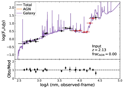
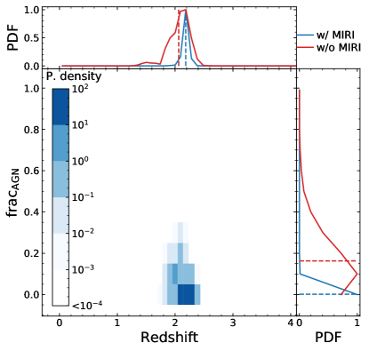
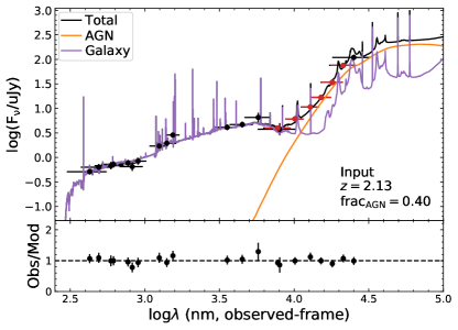
Fig. 11 displays the fitting results for an example source. Note that the MIRI bands cover the PAH emission feature, which can be used as a robust redshift indicator and constrains the nature of the IR emission. Including the MIRI data greatly improves both redshift and constraints, compared to the fitting results without MIRI. In particular, MIRI facilities a constraint on , where data that lack MIRI provide almost no information. This is because MIRI covers the shape of the emission associated with the hot-dust heated by the AGN (§1).
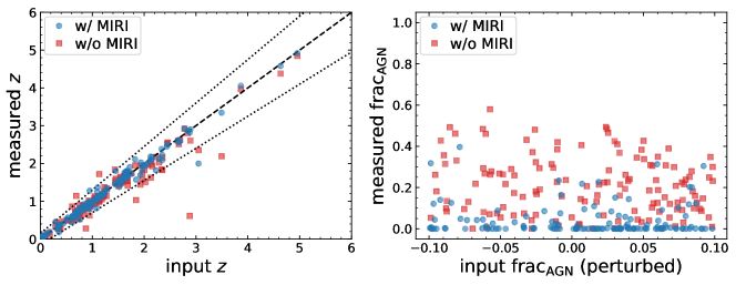
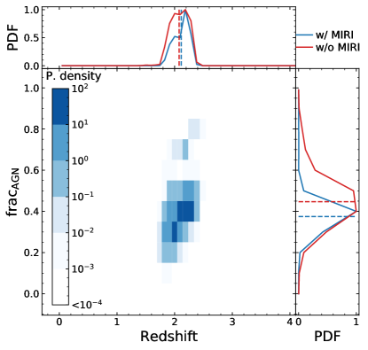
In Fig. 12, we compare the x-cigale redshift and with the input values (§2.2). Following the convention in the literature (e.g., Yang et al., 2014), we adopt fractional redshift uncertainty, , where and and are x-cigale output and input-model redshifts, respectively. We calculate the median and of as well as the outlier fraction (sources with ). These results are marked in Fig. 12. All of the three quantities (median, , and ) are improved significantly after using MIRI. Notably, drops from 10% to 1.5% thanks to MIRI.
One factor for the photo- improvement is likely the capture of PAH emission by MIRI (e.g., Fig. 1). We note that the typical PAH emission is sufficiently strong to be detected by our MIRI filters. For example, the 6.2 m line has a typical rest-frame equivalent width (EW) of m in our galaxy-dust models of Dale et al. (2014) (see, e.g., Armus et al. 2007; Spoon et al. 2007 for similar values). This EW translates to a flux excess of for a galaxy (Fig. 1).666 where is the rest-frame EW and is the filter width (e.g., Papovich et al., 2001). This value is significantly larger than our sources’ photometric uncertainties (–0.22 mag; §3.2.2). The m PAH EW is typically times wider than the m one (e.g., Stierwalt et al., 2014), and thus the former will even have a stronger impact on our MIRI photometry than the latter. We note that the observed EW grows with redshift as so the effects of PAHs on the MIRI bands are more substantive toward higher redshift.
We also calculate the median and values of as shown in Fig. 12. With MIRI, the median and of are 0.002 and 0.003, respectively, both close to the 0. This result indicates tight constraints on the AGN component. Without MIRI, the constraints are poor, and the median and are 0.200 and 0.155, respectively, indicating that the constraints on the AGN component are poor. The significant role of MIRI in constraining AGN highlights its ability of sampling the emission from AGN-heated hot dust (e.g., Figs. 1 and 11). Without MIRI, there is large gap in coverage from IRAC 8 µm to MIPS 24 µm, which is unable to probe the hot dust heated by the AGN, and thus the constraints on the AGN component are much weaker (e.g., Fig. 11). Specifically, surveys that include multiple MIRI bands will be very effective at identifying galaxies without AGN emission.
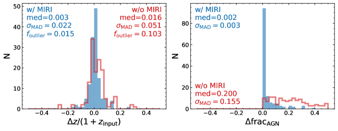
Because the AGN hot-dust emission typically peaks at rest-frame m (e.g., Fig. 3), it is possible that the constraints on become weaker at high redshifts, when the bulk of AGN emission shifts out of the MIRI coverage. To investigate this redshift dependence, we show the distributions of for different redshift bins in Fig. 13. The constraints on are excellent up to , with median and both below . At higher redshifts (), the constraints become substantially weaker as expected as the mid-IR features associated with hot-dust from the AGN shift to higher wavelengths than can be probed by even MIRI. The photo- quality also appears to drop at , although the high- sample size is not sufficiently large for a solid conclusion. The relatively poor photo- quality at high-, if true, could result from the fact that the PAH features also shift to wavelength beyond those covered by MIRI.
3.3.3 Fitting results for galaxy-AGN mixed models
In this section, we present the SED-fitting results for the simulation sets of hypothetical galaxy-AGN mixed models with different positive values of input (§2.2.2). Fig. 14 displays an example SED fitting and PDFs for a source with model . After using MIRI data, the projected 1D PDFs of both redshift and become narrower.
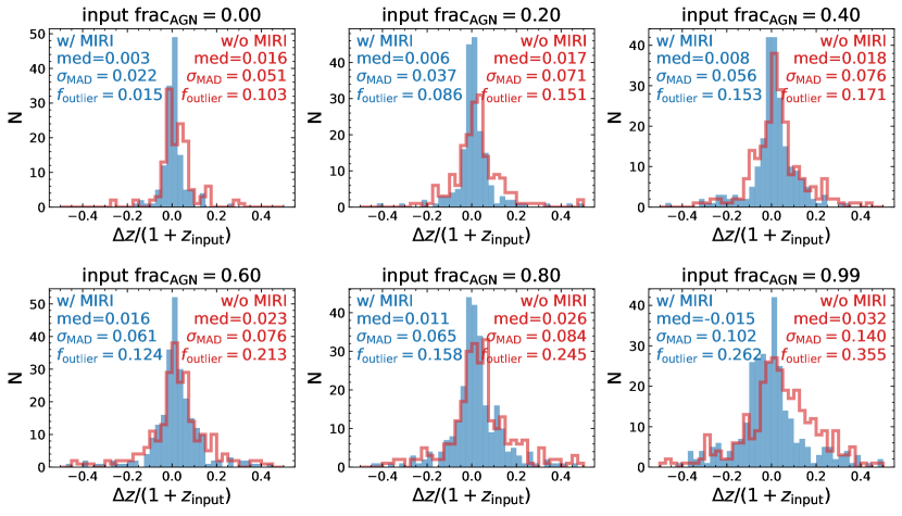
In Fig. 15, we compare the distribution of redshift uncertainties from the fittings with and without MIRI data for different model-input . The redshift accuracy is improved after using MIRI data for each case, as both the scatter and outlier fraction improve with the inclusion of MIRI data. The photo- scatter, , increases as the input increases. This is because, as AGN strength rises, the PAH features (used as redshift indicator) becomes weaker in the SED (see Fig. 3). Another reason is that we select more optically faint objects for higher , as our selection is based on mid-IR (detected in MIRI bands; §3.3). The optical flux uncertainties are larger for these optically faint sources. Regardless, there is appreciable gain when including the MIRI bands.
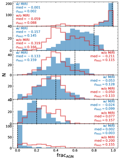
Fig. 16 shows the fitting results of . With MIRI, the dispersion of is remarkably small () for the cases of pure-galaxy () and AGN-dominant (), and it is much larger () for the intermediate cases. This is expected, as in the two extreme cases ( or 0.99), the SED features of galaxy or AGN are dominant. In contrast, when is intermediate, the total SED has mixed features of galaxy and AGN, and the SED decomposition is challenging. These sources would likely be considered “composites” in previous studies (e.g., Kirkpatrick et al., 2017).
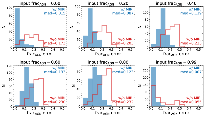
At first glance, for model and , it may appear that the accuracy of does not change significantly after using MIRI data. However, this is misleading. This is because the Bayesian output value in x-cigale is calculated as the PDF-weighted mean (see §4.3 of Boquien et al. 2019), and this produces a median that tends to be located near the center of the parametric range (0.5 for ) in the case that the constraints are weak. Considering the extreme case when the model and the PDF is totally flat, the Bayesian will be exactly the same as the model value, although the constraints on is none. The Bayesian values (dashed lines) are similar for the fitting with and without MIRI, but the PDFs for individual objects is much narrower after using MIRI data. Therefore, sometimes it is not sufficient to use the mean values from the PDF only, and the errors (PDF-weighted standard deviation; §4.3 of Boquien et al. 2019) calculated by x-cigale may serve as a necessary diagnostic. Fig. 17 displays the error distributions for all model configurations. Indeed, for all model (including and ), the median of uncertainties always becomes smaller after using the MIRI data, showing that the constraint on becomes tighter with MIRI. Quantitatively, MIRI data improves the accuracy by a factor of for the case of AGN-galaxy composite input (see Fig. 17).
3.3.4 Constraints on AGN accretion power with MIRI
In §3.3.3, we assess the SED-fitting quality of for the cases where an hypothetical AGN is present in the input models. describes the relative luminosities of AGN vs. galaxy in terms of total IR luminosity. It is understandable that the fitted still has significant scatter even using MIRI data, because we do not have far-IR photometry to tightly constrain the galaxy cold-dust emission, which also affects .
However, it is often useful to obtain absolute AGN luminosities in AGN studies, as black-hole (BH) accretion rates can be estimated from the absolute luminosities (e.g., Ni et al., 2019, 2020; Yang et al., 2019). x-cigale is able to estimate the intrinsic AGN accretion disk luminosity, (i.e., “agn.accretion_power” in the output; Yang et al. 2020). The SKIRTOR AGN model in x-cigale adopts anisotropic disk emission, and is calculated averaging over all viewing angles. Note that the is numerically equivalent to the angle-averaged obscured disk dust luminosity, as SKIRTOR is a physical model obeying energy conservation.
We compare the measured and model-input in Fig. 18 for the simulation sets of different input (§2.2.2). The median and for all cases are dex and dex, respectively (see Fig. 18). Therefore, we can reliably recover from SED fitting of the photometric data of MIRI (and other bands). In the future, MIRI photometric surveys can be widely used in the studies of BH accretion and evolution across cosmic history (§4.2). From Fig. 18, the quality of becomes slightly better toward higher , indicating that the constraint on AGN power is better for sources whose AGN SED component is more dominant in infrared.
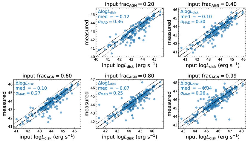
Therefore, in addition to the constraints on , the x-cigale results also provide reliable constraints on the BH accretion power which is a useful quantity for AGN studies.
4 Discussion
4.1 Comparison to Kirkpatrick et al. (2017)
Kirkpatrick et al. (2017) were one of the first to evaluate the use of MIRI to classify and characterize AGN and star-formation in distant galaxies. Their classification scheme is based on MIRI color-color diagrams, and demonstrated that MIRI can identify objects whose IR emission is powered by star-formation, AGN, and composite cases. The method here uses x-cigale and SED-fitting and improves on this previous work as it uses all the available MIRI bands, and measures simultaneously the photometric redshift and galaxy properties simultaneously, providing PDF for each parameter.
We provide here a qualitative comparison between the two methods. Kirkpatrick et al. 2017 derived a parameter (fractional AGN contribution to the rest-frame 5–15 m SED, where the superscript denotes these are derived by Kirkpatrick et al. 2017). They then divided their source SEDs into three classes, i.e., galaxy (), composite (), and AGN (), and define an empirical color-color scheme to classify simulated sources into these classes. They find that their color-color scheme is able to reach a high accuracy level of (galaxy), 76% (composite), and 87% (AGN).
The thresholds and above roughly correspond to our and , respectively (the exact conversions vary from model to model). Therefore, to compare with Kirkpatrick et al. (2017), we choose , , and as the criteria for the galaxy, composite, and AGN classes in our analysis. Under these criteria, for our simulation set of pure-galaxy input models (§2.2.1), 88% sources are correctly classified as a (star-formation-dominated) “galaxy”. (i.e., the in x-cigale output below 0.1; Fig. 12). For the input models of (i.e., the composite models, §2.2.2), the classification accuracy is 72% (Fig. 15). For the input models of , 0.8, and 0.99 (i.e., the AGN models), the success rates are 77%, 90%, and 99%, respectively. Therefore, there is a high degree of overlap between the method of Kirkpatrick et al. (2017) and our SED-fitting method here.
Again, we note that the classifications above are for the comparison with Kirkpatrick et al. (2017) only. The method of Kirkpatrick et al. (2017) is straightforward: one just needs to apply a suitable color-color scheme depending on the source’s redshift which can be spec- (if available) or photo-. The qualitative classification results can be obtained instantaneously. Our SED fitting of x-cigale is a quantitative method that yields PDF-based property estimation as well as best-fit SEDs.
Another advantage of our x-cigale method is that the redshift does need to be known a priori, and x-cigale will fit simultaneously for the redshift and other parameters (including ). This feature is extremely valuable for deep-field sources whose spec- are challenging to measure.
The x-cigale run time for our simulated MIRI pointing (a few hundred sources) is hour on a typical desktop/laptop. The run time will still be acceptable ( day) even for a large sample of a million sources, thanks to the efficient parallel algorithm of x-cigale (Boquien et al., 2019).
4.2 Comparison with X-ray AGN selection
X-ray observations are effective in AGN identification (e.g., Brandt & Alexander, 2015; Xue, 2017). Strong X-ray emission is almost a universal property of the BH accretion process, and galactic processes (e.g., X-ray binaries and hot gas) can only reach low X-ray luminosities typically below erg s-1. Thanks to these strengths, X-ray surveys have detected numerous AGNs in the distant universe, significantly deepening our understanding of BH evolution across cosmic history (e.g., Civano et al., 2016; Luo et al., 2017; Yang et al., 2018b, a). Like X-ray observations, MIRI can also reliably constrain the AGN accretion power (see §3.3.4). To evaluate the effectiveness of MIRI AGN selection, we compare the sensitivities of MIRI vs. X-ray observations below.
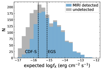
To estimate the equivalent X-ray flux limit in the MIRI selections, first, we calculate model-input AGN 6m luminosities () for all hypothetical sources in all of the simulations (§2.2.2). We then convert to based on the empirical - relation in Stern (2015). We derive the X-ray fluxes (, observed-frame 0.5–7 keV) from assuming an X-ray spectral photon index of (e.g., Yang et al., 2016; Liu et al., 2017). Finally, we decrease these by a factor of 2, which represents the typical X-ray obscuration effect (e.g., Luo et al., 2017). The distributions of MIRI detected and undetected sources are displayed in Fig. 19. From Fig. 19, the MIRI detection becomes significantly incomplete () as the flux drops below erg cm-2 s-1. This is slightly lower than the 50%-completeness limit of CDF-S (Luo et al. 2017; see Fig. 19). Therefore, the deep MIRI exposures (like the multi-hour CEERS/MIRI2) have the potential to identify fainter AGN than even the deepest, highest sensitivity X-ray data achieved so far.
MIRI can even go beyond X-ray for AGN studies, as X-ray AGN selection has a significant weakness. When the obscuration level is high ( cm-2), even hard X-rays can be easily scattered/absorbed, escaping the census of X-ray surveys (e.g., Brandt & Alexander, 2015; Hickox & Alexander, 2018). Such heavily obscured AGNs are often called “Compton-thick” AGNs because of the strong Compton-scattering effect in this high- regime. The analyses of cosmic X-ray background (CXB) suggest that Compton-thick sources may contribute to a large fraction of the AGN population (up to ; e.g., Gilli et al. 2007; Akylas et al. 2012; Ueda et al. 2014). However, the population of Compton-thick AGNs is poorly understood due to the lack of effective selection methods (e.g., Buchner et al., 2015; Li et al., 2019, 2020). The forthcoming MIRI surveys will be a game-changer. The mid-IR emission comes from AGN-heated hot dust, and Compton-thick AGNs likely have abundant obscuring dust (e.g., Georgantopoulos et al., 2011). Therefore, MIRI should be able to detect the missing population of Compton-thick AGNs, and x-cigale can serve as a reliable tool to identify their AGN nature (e.g., Li et al., 2020; Pouliasis et al., 2020).
Assuming the versus intrinsic relation (Stern, 2015) also holds for Compton-thick AGNs, MIRI should be able to detect even many low-luminosity Compton-thick sources according to our sensitivity estimation above. For example, MIRI can sample Compton-thick AGNs with intrinsic down to erg s-1 at (the peak of cosmic AGN activity). This sensitivity is times below the break of the known AGN luminosity function, which is derived based on non-Compton-thick AGNs (e.g., Aird et al., 2010; Ueda et al., 2014). Therefore, future MIRI surveys will allow us to infer a completely new AGN luminosity function for Compton-thick AGNs, shedding light on this mysterious population.
In summary, with a moderate amount of exposure time (such as the 3.6 hours for CEERS/MIRI2), MIRI can already reach a sensitivity level similar to the deepest X-ray survey. MIRI should also be able to identify the Compton-thick population, which is largely missed in X-ray surveys. In the future, MIRI surveys will provide a complete census of the entire population of accreting BHs, enabling unbiased studies of BH evolution across the cosmic history (§3.3.4).
4.3 The effects of different MIRI bands
Our analyses in §3.3 utilizes the full set of simulated MIRI bands from F770W to F2100W. Using all these six bands takes full advantage of the data, and thus yields the tightest possible constraints on source properties. However, there are likely to be MIRI observations in the future that do not have full band coverage as we expect for CEERS. Therefore, understanding the effects on redshifts and galaxy diagnostics using different combinations of MIRI bands is helpful for future survey design and analysis. Below, we investigate the effects of the bluer (F770W, F1000W, and F1280W) and redder (F1500W, F1800W, and F2100W) MIRI bands, respectively. This test is an example of using different band combinations.777Readers may need to know the effects of other band sets for purposes of, e.g., survey planning. We are willing to perform similar assessment for any specific band combination upon e-mail request.
We re-perform the SED fittings in §3.3.2 (pure-galaxy inputs) where we only add the three bluer MIRI bands (F770W, F1000W, F1280W) or the three redder MIRI bands (F1500W, F1800W, F2100W) to the other CANDELS multiband catalogs. These combinations result in photometric accuracies of and outlier fractions of when using the blue/red MIRI bands, respectively. These values are intermediate between those obtained by using none of the MIRI bands versus all MIRI bands (Fig. 12), as expected. The blue MIRI bands improve the photo- accuracy more significantly than the red bands. We attribute the reason to that the blue bands generally have higher sensitivity than the red bands. For example, the median S/Ns in F1000W and F1800W are 6.6 and 3.9, respectively, for our analyzed sources. Notably, the blue bands significantly reduce by a factor of , compared to the case when using only non-MIRI bands. This result is consistent with the findings of Bisigello et al. (2016), who concluded blue MIRI bands (F560W and F770W in their case) can significantly reduce the photo- outliers. Therefore, future photo- surveys could consider including a few MIRI blue bands in their data if possible.
Lastly, we discuss the effects of blue/red MIRI bands on . We re-perform the SED fittings for different inputs (§3.3.2 and §3.3.3) but using the same combinations of only the blue/red MIRI bands, respectively, combined with the other CANDELS multiwavelength bands. As expected, the resulting accuracy of is between those when using none and all MIRI bands (Fig. 16), similar to our finding for the photometric redshifts above. However, in contrast to the photo- results, the accuracy is similar when using either the combination of blue or red MIRI bands. For example, for input , the fitted qualities are and when using the blue/red bands, respectively. We conclude that this is because AGN emission is typically stronger in the red bands than in the blue bands (e.g., Figs. 1 and 14), which enables similar constraining power on the AGN emission and this overcomes the fact that the bluer MIRI bands typically have higher flux sensitivity.
5 Summary and Future Prospects
In this work, we simulate the JWST/MIRI photometric data, and investigate its ability to constrain source properties with SED fitting. Specifically we focus on the ability of surveys with multi-band MIRI imaging to constrain the AGN properties of distant galaxies. Our data processing and results are summarized below.
-
1.
Based on the currently existing broad-band photometry from CANDELS/EGS, we perform SED fitting for the 463 sources within the CEERS/MIRI2 pointing (§2.2). We employ x-cigale to realize the fitting, using pure-galaxy models. In addition, we also add a hypothetical AGN component to the best-fit galaxy SEDs, assuming different fractions of the AGN to the total IR emission (). We obtain model MIRI fluxes for the cases when there is no AGN and when AGN is present, by convolving the model SEDs with the MIRI filters.
-
2.
We simulate the MIRI imaging data with mirisim, using the predicted flux densities above, and adopting Sérsic profiles for the galaxy morphologies (§2.3). We take the raw (Stage 0) data products from the simulation, and reduce them using the jwst calibration pipeline applying custom corrections to the background. We then obtain the dither-merged images for each MIRI band (§3.1). We apply scaling and aperture corrections to the data based on a set of simulated bright point sources (Appendix A). Theses corrections can be refined empirically for real observations of bright calibration stars after launch. We perform PSF-matched photometry with tphot using the existing CANDELS/EGS HST F160W source catalog. We show this achieves depths in the MIRI data similar to those expected in the CEERS using the JWST/ETC(§3.2). The detection rate of sources in the HST catalog by MIRI is high: 75% of the sources are significantly () detected in at least two MIRI bands (for the default case where SEDs assume pure-galaxy models).
-
3.
We perform x-cigale SED fitting, with and without the addition of the MIRI data (§3.3). We focus on the ability of the SED fitting to constrain the photometric redshift and (these are fit simultaneously, and we marginalize of the probability density functions to derive constraints on these parameters). The accuracies of both redshift and are improved significantly after using MIRI data, thanks to the capture of PAH features and AGN hot-dust emission by MIRI. Notably, for the simulation set of pure-galaxy models (which is likely the case for most MIRI sources), can be constrained to the level of with MIRI data, which is times better than the fitting without MIRI data. At the same time, the photo- scatter and outlier fraction are improved by a factor of and , respectively, thanks to MIRI’s capture of PAH emission.
- 4.
-
5.
We assess the AGN-detection sensitivity of MIRI vs. X-ray (§4.2) and find that, for a deep MIRI exposures (such as the CEERS-depth, 3.6-hour data simulated in this work), MIRI can already reach a sensitivity level even slightly higher than the deepest X-ray survey, CDF-S. MIRI should also detect Compton-thick AGNs for which X-ray selection is highly incomplete. Therefore, we conclude that MIRI will provide a complete census of the entire population of accreting BHs, enabling unbiased studies of BH evolution across cosmic history.
-
6.
We discuss the effects of using different MIRI bands in SED fitting (§4.3). In particular, we focus on comparing the bluer (F770W, F1000W, and F1280W) and redder (F1500W, F1800W, and F2100W) bands. We find that the blue bands are more helpful for photo- improvement than the red bands, because the former are more sensitive than the latter. However, the blue and red bands have similar effects in terms of constraining , likely due to the fact that AGN emission is typically stronger in the red bands than in the blue ones.
Although this work focuses on the CEERS/MIRI2 observational strategy, it has general implications for other MIRI extragalactic surveys. For the surveys with the same filters (F770W to F2100W) but different depths, the qualitative conclusions in this paper are likely to hold in general as any MIRI data with similar depth will achieve similar results. The only change is that different exposures will yield different detection limits (e.g., Fig. 2). For example, deeper exposures will be able to detect more faint mid-IR sources at higher fidelity, thereby constraining their source properties (such as photo- and ). For surveys with similar exposures as CEERS/MIRI2 but different band coverage, we have performed an example assessment in §4.3. We are willing to repeat the assessment for any other specific band set upon e-mail request, to satisfy the realistic needs of, e.g., survey planning.
Acknowledgements
We thank the helpful discussions with Jacqueline Antwi-Danso, Emiliano Merlin, Karl Gordon, and the STScI JWST team. We also thank our collaborators on CEERS for their work and contributions to the project. The authors acknowledge the Texas A&M University Brazos HPC cluster and Texas A&M High Performance Research Computing Resources (HPRC, http://hprc.tamu.edu) that contributed to the research reported here. We also acknowledge our collaborators within CEERS for their input in the project. This work acknowledges support from the NASA/ESA/CSA James Webb Space Telescope through the Space Telescope Science Institute, which is operated by the Association of Universities for Research in Astronomy, Incorporated, under NASA contract NAS5-03127. Support for program number JWST-ERS-01345 was provided through a grant from the STScI under NASA contract NAS5-03127. PGP-G acknowledges support from Spanish Government research grant PGC2810-093499-BI00.
In this appendix, we provide addition information about the simulations, modeling, and tests on the MIRI data.
Appendix A Simulated MIRI Data Validation and Aperture Corrections
Both mirisim and pipeline are still in development. This work uses current versions of the available software, but we acknowledge these could be updated prior to the acquisition of JWST data post-launch. One known issue is that the the mirisim and pipeline adopt different MIRI calibration files, which might also affect our simulated MIRI imaging data. Therefore, to investigate potential issues related to mirisim and pipeline, we applied additional tests to validate the imaging data before the photometry-extraction process (§3.2). Below we perform data validation and correction processes based on a set of simulated bright point sources.
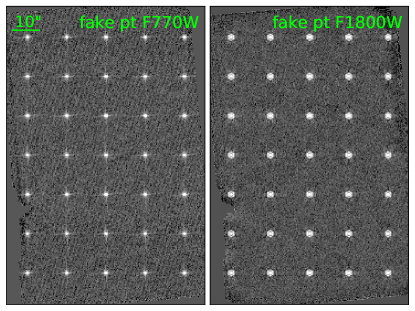
Using mirisim (§2.3), we simulate a grid of bright (but non-saturated) point sources with a signal-to-noise (S/N) of for each MIRI band. The separation between the neighboring sources is , which is sufficiently large to avoid light pollution from neighbors. Fig. 20 displays example simulated images for the MIRI F770W and F1800W bands (where these images have been fully reduced following the procedures in §3.1), where we have repeated this process for all MIRI bands to be obtained for the CEERS/MIRI2 field. These sources have a high S/N of 1000, and thus are less affected by the details of noise in the data-reduction process compared to the realistic faint sources.
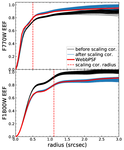
We measure the EEF as a function of radius for each simulated point source at different positions. The EEF at a given radius is calculated as the encircled flux within the radius divided by the model-input flux. The results for F770W and F1800W are displayed in Fig. 21 as examples. The EEFs for the point sources at different positions show slight variations, which is expected given the spatial variations in the background (§3.1). but the scatter is small ( at ). This small scatter indicates that the flat-field correction in pipeline functions well. However, we find systematic offsets between the measured EEFs for these point sources compared to the theoretical PSF EEF from webbpsf (version 0.90).888https://www.stsci.edu/jwst/science-planning/proposal-planning-toolbox/psf-simulation-tool The specific reason is possibly due to the inconsistencies between the MIRI calibration files adopted by mirisim and pipeline (K. Gordon 2020, private communication). It is also possible that one of the simulation steps are truncating the wings of the PSF. As these possibilities are associated with the production of the simulations, they are unlikely to be present in the real JWST data. Here, for our purposes we measure the systematic offset as a “scaling correction”, which we then apply to the flux densities in MIRI that we measure. This scaling “correction factor” is calculated as,
| (A1) |
where is the median of point-source EEF at (the radius where PSF EEF; see Fig. 21). The value 0.8 is chosen, because most of the light is encircled within and the pixels are still source-dominated instead of background-dominated at . The values of are all within 10% of unity and range from 0.87 (F1800W) to 1.08 (F770W). We apply the scaling correction by multiplying all pixel values by a factor of for each MIRI band. After this procedure, the point-source EEFs become similar to the PSF EEF as displayed in Fig. 21.
Besides the scaling correction above, we also need to consider aperture corrections. This is because the PSF faint wings extend to large radii, and can contribute to the background (Fig. 21). We calculate the aperture-correction by comparing the total (input/true) flux density to the averaged measured flux density. The aperture-correction factor is,
| (A2) |
where is the PSF EEF at 1.5. We choose the radius of as a fiducial value as beyond this radius the EEF has little growth (see Fig. 21). We apply the aperture correction by multiplying the measured source fluxes by a factor of . As expected, is higher for longer wavelengths which correspond to more extended PSF. The values of increase with PSF FWHM (which scales with wavelength) and range from 1.10 (F770W) to 1.19 (F2100W).
We note that the correction procedures above are not limited to the simulated MIRI data and can be applied to real MIRI data. After the launch of JWST, some bright “standard stars” with known mid-IR fluxes can play the same role as the simulated point sources in this work. In fact, some key calibration programs focusing on standard stars have already been scheduled for the upcoming Cycle 1.999https://jwst-docs.stsci.edu/data-processing-and-calibration-files/absolute-flux-calibration
After the corrections above, we extract photometry for the simulated point sources using tphot (see §3.2). We assess the photometry quality by comparing the measured magnitudes and the model-input magnitudes. Fig. 22 shows the distribution of the magnitude offsets for F770W and F1800W as examples. The systematics and scatters are both mag for all MIRI bands, indicate that our photometric corrections above and tphot measurements are reliable.
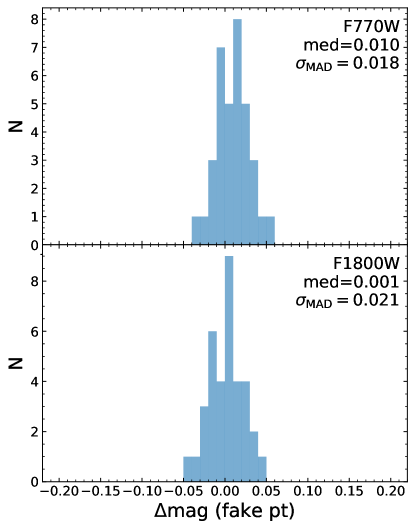
Appendix B The simulation of F160W imaging data
To extract the photometry on the simulated MIRI images, we also need to simulated F160W images that have source morphologies consistent with MIRI morphologies (see §3.2.1). Note that we use the simulated HST image only to measure MIRI flux densities from TPHOT (we use the real F160W source fluxes and errors from the CANDELS/EGS catalog when fitting the SEDs in §2.2.1). First, we create an empty image covering the same region as the simulated MIRI fields, with pixel size set to (the same as CANDELS survey). We then position all sources (Stefanon et al., 2017) within the FOV on the image. The fluxes are set to the observed F160W fluxes in the Stefanon et al. (2017) catalog, and the morphologies use the same Sérsic model parameters (from the van der Wel et al. 2012 catalog) that are used for the mirisim input above. In addition, for a point-like sources, we allow slight shifts to center the pixel at the pixel nearest to the source position; for a Sérsic source, we generate its profile utilizing the sersic2d function of astropy (Astropy Collaboration et al., 2018), which allows fractional pixel positions. Next, we convolve the image with the F160W point spread function (PSF) derived by the 3DHST team (Momcheva et al., 2016). We perform this convolution process with the convolve_fft function of astropy. Finally, we add a random Gaussian noise to each pixel with an amplitude from the RMS map produced by the CANDELS team (Grogin et al., 2011; Koekemoer et al., 2011). Fig. 23 compares the cutouts of the original/simulated F160W images and two MIRI-band images. For the galaxy near the center, the simulated and original F160W profiles are obviously different, since a Sérsic profile, as a proxy, cannot reproduce the complex morphological feature of spiral arms. As expected, the MIRI images have the similar profiles as the simulated F160W image, because they share the same input Sérsic profile.
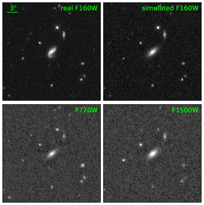
Appendix C Comparison between source extractor and tphot photometry
source extractor (Bertin & Arnouts, 1996) is widely used for photometry extraction (e.g., Caputi, 2013; Yang et al., 2014; Kauffmann et al., 2020). Therefore, it is instructive to test the performance of source extractor on our simulated MIRI images. Using F1500W as an example, we perform source extractor photometry and compare the resulting quality with that from tphot below. The results are similar for other MIRI bands.
The “AUTO” mode photometry in source extractor provides an estimation of the bulk of the total flux based on an adaptive-aperture algorithm (Kron, 1980). The AUTO method automatically adjusts the size and shape of an elliptical aperture and it works best for bright resolved sources with high S/Ns. However, for a faint low-S/N source, the aperture size (and thus the resulting flux) could be systematically underestimated (Bertin & Arnouts, 1996). This issue can be alleviated by adopting a circular photometry aperture of a fixed size for faint sources. Therefore, we adopt a strategy of choosing the brighter one of the AUTO and fixed-aperture fluxes (after corrections) for each source.
We run source extractor on the same F1500W image as in our tphot run (§3.2.2; pure-galaxy inputs). Our source extractor run adopts the parameters listed in Table. 3. The aperture size (PHOTO_APERTURES ) corresponds to 80% point-source EEF in F1500W, and thus we correct the resulting aperture fluxes by a factor of 1/0.8 to estimate the total fluxes. Based on our choice of “PHOTO_AUTOPARAMS”, the AUTO flux is expected to recover of the total flux on average (Bertin & Arnouts, 1996). Therefore, we correct the resulting AUTO fluxes by a factor of 1/0.94 to obtain the total. The run detects 379 F1500W sources. We associate them with the input source catalog using a matching radius, and this procedure results in 177 matches. We assess the source extractor photometry quality using these 177 sources below.
Fig. 24 compares the resulting source extractor magnitudes with the input magnitudes. The right panel of Fig. 24 displays the error function of both source extractor and tphot photometry. The tphot photometric uncertainties are generally smaller than the source extractor uncertainties at a given magnitude, indicating that tphot photometry has superior quality than source extractor photometry. Another advantage of tphot is that it can estimate the fluxes of all sources provided in the high-resolution prior catalog (see §3.2.1), and this provides valuable information for the mid-IR emission in these sources. However, source extractor could miss many sources that are faint in the photometric band. For example, our source extractor run misses 53% of the sources in the input catalog. These sources are all present in our tphot catalog.
Fig. 25 directly compares source extractor vs. tphot magnitudes for point/ and sources (similar as Fig. 9). The systematic differences (as indicated by the median) between source extractor and tphot magnitudes are generally small ( mag). This systematic consistency indicates that, like tphot, source extractor also misses the light from the faint extended wings for sources (see §3.2.2).
| Parameter | Value |
|---|---|
| DETECT_MINAREA | 5 |
| FILTER | Y |
| FILTER_NAME | gauss_5.0_9x9.conv |
| PHOTO_APERTURES | 31 |
| PHOTO_AUTOPARAMS | 2.5, 3.5 |
| BACK_SIZE | 64 |
| BACK_FILTERSIZE | 6 |
| BACKPHOTO_TYPE | LOCAL |
| BACKPHOTO_THICK | 40 |
Note. — For parameters not listed here, we use default values.
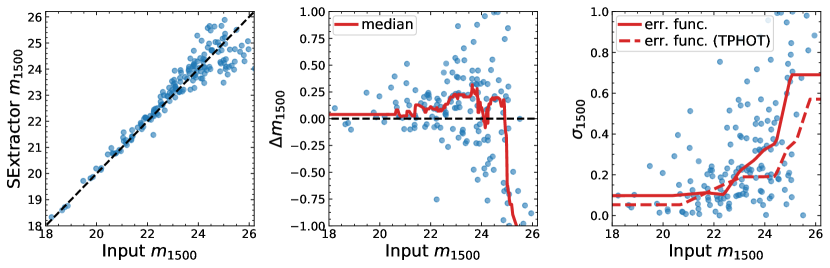
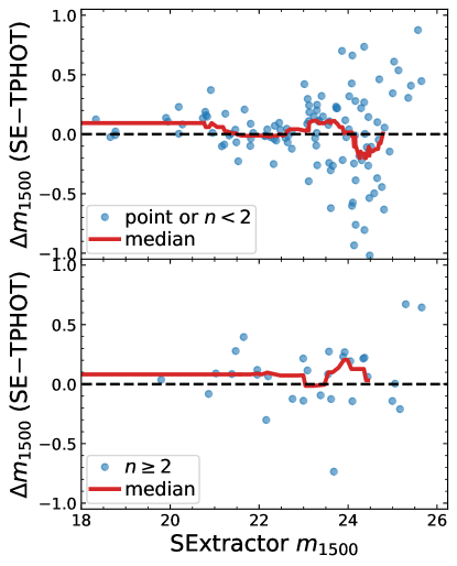
Appendix D Complete Comparisons between Input and Measured Flux Densities for all MIRI bands
In this appendix, Fig. 26 shows the comparison between input and measured flux densities for all the MIRI bands (and is similar to Fig. 8 above). Figure 24 compares the results dividing the sample by morphology (Sérsic index) for all bands (and is similar to Fig. 9 above).
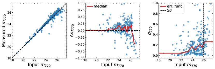
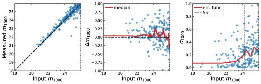
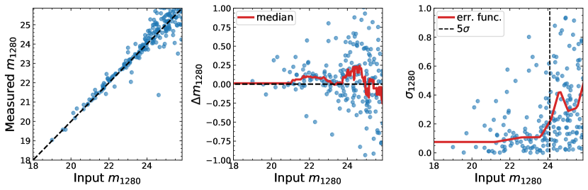

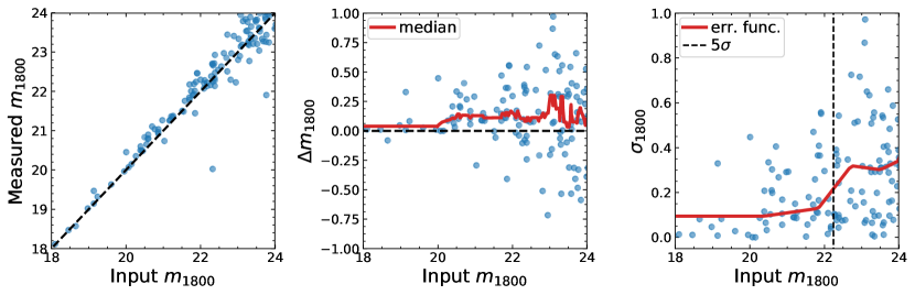
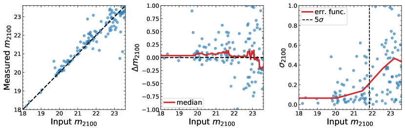
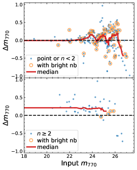
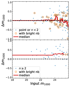
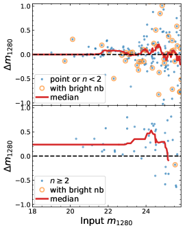
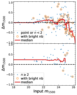
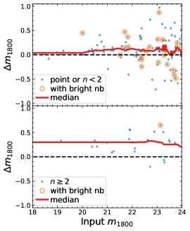
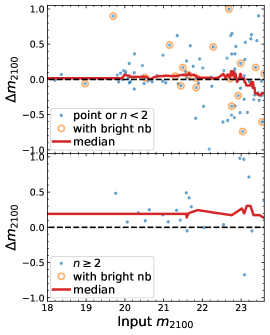
References
- Aird et al. (2010) Aird, J., Nandra, K., Laird, E. S., et al. 2010, MNRAS, 401, 2531, doi: 10.1111/j.1365-2966.2009.15829.x
- Akylas et al. (2012) Akylas, A., Georgakakis, A., Georgantopoulos, I., Brightman, M., & Nandra, K. 2012, A&A, 546, A98, doi: 10.1051/0004-6361/201219387
- Alberts et al. (2020) Alberts, S., Rujopakarn, W., Rieke, G. H., Jagannathan, P., & Nyland, K. 2020, ApJ, 901, 168, doi: 10.3847/1538-4357/abb1a0
- Alexander et al. (2008) Alexander, D. M., Chary, R.-R., Pope, A., et al. 2008, ApJ, 687, 835, doi: 10.1086/591928
- Alonso-Herrero et al. (2006) Alonso-Herrero, A., Pérez-González, P. G., Alexand er, D. M., et al. 2006, ApJ, 640, 167, doi: 10.1086/499800
- Antonucci (1993) Antonucci, R. 1993, ARA&A, 31, 473, doi: 10.1146/annurev.aa.31.090193.002353
- Armus et al. (2007) Armus, L., Charmandaris, V., Bernard-Salas, J., et al. 2007, ApJ, 656, 148, doi: 10.1086/510107
- Ashby et al. (2018) Ashby, M. L. N., Caputi, K. I., Cowley, W., et al. 2018, ApJS, 237, 39, doi: 10.3847/1538-4365/aad4fb
- Asmus (2019) Asmus, D. 2019, arXiv e-prints, arXiv:1908.03552. https://arxiv.org/abs/1908.03552
- Assef et al. (2013) Assef, R. J., Stern, D., Kochanek, C. S., et al. 2013, ApJ, 772, 26, doi: 10.1088/0004-637X/772/1/26
- Astropy Collaboration et al. (2018) Astropy Collaboration, Price-Whelan, A. M., Sipőcz, B. M., et al. 2018, AJ, 156, 123, doi: 10.3847/1538-3881/aabc4f
- Azadi et al. (2018) Azadi, M., Coil, A., Aird, J., et al. 2018, ApJ, 866, 63, doi: 10.3847/1538-4357/aad3c8
- Barbary (2016) Barbary, K. 2016, The Journal of Open Source Software, 1, 58, doi: 10.21105/joss.00058
- Bertin & Arnouts (1996) Bertin, E., & Arnouts, S. 1996, A&AS, 117, 393
- Bisigello et al. (2016) Bisigello, L., Caputi, K. I., Colina, L., et al. 2016, ApJS, 227, 19, doi: 10.3847/0067-0049/227/2/19
- Bisigello et al. (2017) —. 2017, ApJS, 231, 3, doi: 10.3847/1538-4365/aa7a14
- Bonato et al. (2017) Bonato, M., Sajina, A., De Zotti, G., et al. 2017, ApJ, 836, 171, doi: 10.3847/1538-4357/aa5c85
- Boquien et al. (2019) Boquien, M., Burgarella, D., Roehlly, Y., et al. 2019, A&A, 622, A103, doi: 10.1051/0004-6361/201834156
- Boucaud et al. (2016) Boucaud, A., Bocchio, M., Abergel, A., et al. 2016, A&A, 596, A63, doi: 10.1051/0004-6361/201629080
- Brandt & Alexander (2015) Brandt, W. N., & Alexander, D. M. 2015, A&A Rev., 23, 1, doi: 10.1007/s00159-014-0081-z
- Bruzual & Charlot (2003) Bruzual, G., & Charlot, S. 2003, MNRAS, 344, 1000, doi: 10.1046/j.1365-8711.2003.06897.x
- Buchner et al. (2015) Buchner, J., Georgakakis, A., Nandra, K., et al. 2015, ApJ, 802, 89, doi: 10.1088/0004-637X/802/2/89
- Calzetti et al. (2000) Calzetti, D., Armus, L., Bohlin, R. C., et al. 2000, ApJ, 533, 682, doi: 10.1086/308692
- Caputi (2013) Caputi, K. I. 2013, ApJ, 768, 103, doi: 10.1088/0004-637X/768/2/103
- Chabrier (2003) Chabrier, G. 2003, ApJ, 586, L133, doi: 10.1086/374879
- Chang et al. (2017) Chang, Y.-Y., Le Floc’h, E., Juneau, S., et al. 2017, ApJS, 233, 19, doi: 10.3847/1538-4365/aa97da
- Chary et al. (2007) Chary, R.-R., Teplitz, H. I., Dickinson, M. E., et al. 2007, ApJ, 665, 257, doi: 10.1086/519243
- Civano et al. (2016) Civano, F., Marchesi, S., Comastri, A., et al. 2016, ApJ, 819, 62, doi: 10.3847/0004-637X/819/1/62
- Clements et al. (2011) Clements, D. L., Bendo, G., Pearson, C., et al. 2011, MNRAS, 411, 373, doi: 10.1111/j.1365-2966.2010.17689.x
- Daddi et al. (2007a) Daddi, E., Dickinson, M., Morrison, G., et al. 2007a, ApJ, 670, 156, doi: 10.1086/521818
- Daddi et al. (2007b) Daddi, E., Alexander, D. M., Dickinson, M., et al. 2007b, ApJ, 670, 173, doi: 10.1086/521820
- Dale et al. (2014) Dale, D. A., Helou, G., Magdis, G. E., et al. 2014, ApJ, 784, 83, doi: 10.1088/0004-637X/784/1/83
- Del Moro et al. (2016) Del Moro, A., Alexander, D. M., Bauer, F. E., et al. 2016, MNRAS, 456, 2105, doi: 10.1093/mnras/stv2748
- Dickinson et al. (2006) Dickinson, M., Alexander, D., Bell, E., et al. 2006, A Deep-Wide Far-Infrared Survey of Cosmological Star Formation and AGN Activity, Spitzer Proposal
- Dole et al. (2004) Dole, H., Rieke, G. H., Lagache, G., et al. 2004, ApJS, 154, 93, doi: 10.1086/422690
- Donley et al. (2012) Donley, J. L., Koekemoer, A. M., Brusa, M., et al. 2012, ApJ, 748, 142, doi: 10.1088/0004-637X/748/2/142
- Draine & Li (2007) Draine, B. T., & Li, A. 2007, ApJ, 657, 810, doi: 10.1086/511055
- Finkelstein et al. (2017) Finkelstein, S. L., Dickinson, M., Ferguson, H. C., et al. 2017, The Cosmic Evolution Early Release Science (CEERS) Survey, JWST Proposal ID 1345. Cycle 0 Early Release Scienc
- Georgantopoulos et al. (2011) Georgantopoulos, I., Rovilos, E., Akylas, A., et al. 2011, A&A, 534, A23, doi: 10.1051/0004-6361/201117400
- Gilli et al. (2007) Gilli, R., Comastri, A., & Hasinger, G. 2007, A&A, 463, 79, doi: 10.1051/0004-6361:20066334
- Glasse et al. (2015) Glasse, A., Rieke, G. H., Bauwens, E., et al. 2015, PASP, 127, 686, doi: 10.1086/682259
- Grogin et al. (2011) Grogin, N. A., Kocevski, D. D., Faber, S. M., et al. 2011, ApJS, 197, 35, doi: 10.1088/0067-0049/197/2/35
- Häussler et al. (2007) Häussler, B., McIntosh, D. H., Barden, M., et al. 2007, ApJS, 172, 615, doi: 10.1086/518836
- Hickox & Alexander (2018) Hickox, R. C., & Alexander, D. M. 2018, ARA&A, 56, 625, doi: 10.1146/annurev-astro-081817-051803
- Kauffmann et al. (2020) Kauffmann, O. B., Le Fèvre, O., Ilbert, O., et al. 2020, A&A, 640, A67, doi: 10.1051/0004-6361/202037450
- Kennicutt (1998) Kennicutt, Jr., R. C. 1998, ApJ, 498, 541, doi: 10.1086/305588
- Kirkpatrick et al. (2015) Kirkpatrick, A., Pope, A., Sajina, A., et al. 2015, ApJ, 814, 9, doi: 10.1088/0004-637X/814/1/9
- Kirkpatrick et al. (2017) Kirkpatrick, A., Alberts, S., Pope, A., et al. 2017, ApJ, 849, 111, doi: 10.3847/1538-4357/aa911d
- Klaassen et al. (2020) Klaassen, P. D., Geers, V. C., Beard, S. M., et al. 2020, arXiv e-prints, arXiv:2010.15710. https://arxiv.org/abs/2010.15710
- Koekemoer et al. (2011) Koekemoer, A. M., Faber, S. M., Ferguson, H. C., et al. 2011, ApJS, 197, 36, doi: 10.1088/0067-0049/197/2/36
- Komatsu et al. (2011) Komatsu, E., Smith, K. M., Dunkley, J., et al. 2011, ApJS, 192, 18, doi: 10.1088/0067-0049/192/2/18
- Kron (1980) Kron, R. G. 1980, ApJS, 43, 305, doi: 10.1086/190669
- Laidler et al. (2007) Laidler, V. G., Papovich, C., Grogin, N. A., et al. 2007, PASP, 119, 1325, doi: 10.1086/523898
- Leitherer et al. (2002) Leitherer, C., Li, I. H., Calzetti, D., & Heckman, T. M. 2002, ApJS, 140, 303, doi: 10.1086/342486
- Li et al. (2019) Li, J., Xue, Y., Sun, M., et al. 2019, ApJ, 877, 5, doi: 10.3847/1538-4357/ab184b
- Li et al. (2020) —. 2020, arXiv e-prints, arXiv:2008.05863. https://arxiv.org/abs/2008.05863
- Liu et al. (2017) Liu, T., Tozzi, P., Wang, J.-X., et al. 2017, ApJS, 232, 8, doi: 10.3847/1538-4365/aa7847
- Luo et al. (2017) Luo, B., Brandt, W. N., Xue, Y. Q., et al. 2017, ApJS, 228, 2, doi: 10.3847/1538-4365/228/1/2
- Lutz et al. (2011) Lutz, D., Poglitsch, A., Altieri, B., et al. 2011, A&A, 532, A90, doi: 10.1051/0004-6361/201117107
- Małek et al. (2014) Małek, K., Pollo, A., Takeuchi, T. T., et al. 2014, A&A, 562, A15, doi: 10.1051/0004-6361/201321665
- Merlin et al. (2015) Merlin, E., Fontana, A., Ferguson, H. C., et al. 2015, A&A, 582, A15, doi: 10.1051/0004-6361/201526471
- Merlin et al. (2016) Merlin, E., Bourne, N., Castellano, M., et al. 2016, A&A, 595, A97, doi: 10.1051/0004-6361/201628751
- Merloni et al. (2014) Merloni, A., Bongiorno, A., Brusa, M., et al. 2014, MNRAS, 437, 3550, doi: 10.1093/mnras/stt2149
- Messias et al. (2012) Messias, H., Afonso, J., Salvato, M., Mobasher, B., & Hopkins, A. M. 2012, ApJ, 754, 120, doi: 10.1088/0004-637X/754/2/120
- Momcheva et al. (2016) Momcheva, I. G., Brammer, G. B., van Dokkum, P. G., et al. 2016, ApJS, 225, 27, doi: 10.3847/0067-0049/225/2/27
- Nandra et al. (2015) Nandra, K., Laird, E. S., Aird, J. A., et al. 2015, ApJS, 220, 10, doi: 10.1088/0067-0049/220/1/10
- Netzer (2015) Netzer, H. 2015, ARA&A, 53, 365, doi: 10.1146/annurev-astro-082214-122302
- Ni et al. (2019) Ni, Q., Yang, G., Brandt, W. N., et al. 2019, MNRAS, 490, 1135, doi: 10.1093/mnras/stz2623
- Ni et al. (2020) Ni, Q., Brandt, W. N., Yang, G., et al. 2020, arXiv e-prints, arXiv:2007.04987. https://arxiv.org/abs/2007.04987
- Oke & Gunn (1983) Oke, J. B., & Gunn, J. E. 1983, ApJ, 266, 713, doi: 10.1086/160817
- Oliver et al. (2012) Oliver, S. J., Bock, J., Altieri, B., et al. 2012, MNRAS, 424, 1614, doi: 10.1111/j.1365-2966.2012.20912.x
- Papovich et al. (2001) Papovich, C., Dickinson, M., & Ferguson, H. C. 2001, ApJ, 559, 620, doi: 10.1086/322412
- Papovich et al. (2004) Papovich, C., Dole, H., Egami, E., et al. 2004, ApJS, 154, 70, doi: 10.1086/422880
- Papovich et al. (2007) Papovich, C., Rudnick, G., Le Floc’h, E., et al. 2007, ApJ, 668, 45, doi: 10.1086/521090
- Pirzkal et al. (2012) Pirzkal, N., Rothberg, B., Nilsson, K. K., et al. 2012, ApJ, 748, 122, doi: 10.1088/0004-637X/748/2/122
- Pouliasis et al. (2020) Pouliasis, E., Mountrichas, G., Georgantopoulos, I., et al. 2020, MNRAS, 495, 1853, doi: 10.1093/mnras/staa1263
- Rieke et al. (2019) Rieke, G., Alberts, S., Shivaei, I., Colina, L., & Nørgaard-Nielsen, H. U. 2019, BAAS, 51, 11
- Salim et al. (2007) Salim, S., Rich, R. M., Charlot, S., et al. 2007, ApJS, 173, 267, doi: 10.1086/519218
- Sersic (1968) Sersic, J. L. 1968, Atlas de Galaxias Australes
- Shipley et al. (2016) Shipley, H. V., Papovich, C., Rieke, G. H., Brown, M. J. I., & Moustakas, J. 2016, ApJ, 818, 60, doi: 10.3847/0004-637X/818/1/60
- Shivaei et al. (2017) Shivaei, I., Reddy, N. A., Shapley, A. E., et al. 2017, ApJ, 837, 157, doi: 10.3847/1538-4357/aa619c
- Spoon et al. (2007) Spoon, H. W. W., Marshall, J. A., Houck, J. R., et al. 2007, ApJ, 654, L49, doi: 10.1086/511268
- Stalevski et al. (2012) Stalevski, M., Fritz, J., Baes, M., Nakos, T., & Popović, L. Č. 2012, MNRAS, 420, 2756, doi: 10.1111/j.1365-2966.2011.19775.x
- Stalevski et al. (2016) Stalevski, M., Ricci, C., Ueda, Y., et al. 2016, MNRAS, 458, 2288, doi: 10.1093/mnras/stw444
- Stalevski et al. (2019) Stalevski, M., Tristram, K. R. W., & Asmus, D. 2019, MNRAS, 484, 3334, doi: 10.1093/mnras/stz220
- Stefanon et al. (2017) Stefanon, M., Yan, H., Mobasher, B., et al. 2017, ApJS, 229, 32, doi: 10.3847/1538-4365/aa66cb
- Stern (2015) Stern, D. 2015, ApJ, 807, 129, doi: 10.1088/0004-637X/807/2/129
- Stern et al. (2005) Stern, D., Eisenhardt, P., Gorjian, V., et al. 2005, ApJ, 631, 163, doi: 10.1086/432523
- Stern et al. (2012) Stern, D., Assef, R. J., Benford, D. J., et al. 2012, ApJ, 753, 30, doi: 10.1088/0004-637X/753/1/30
- Stierwalt et al. (2014) Stierwalt, S., Armus, L., Charmandaris, V., et al. 2014, ApJ, 790, 124, doi: 10.1088/0004-637X/790/2/124
- Tielens (2008) Tielens, A. G. G. M. 2008, ARA&A, 46, 289, doi: 10.1146/annurev.astro.46.060407.145211
- Ueda et al. (2014) Ueda, Y., Akiyama, M., Hasinger, G., Miyaji, T., & Watson, M. G. 2014, ApJ, 786, 104, doi: 10.1088/0004-637X/786/2/104
- Urry & Padovani (1995) Urry, C. M., & Padovani, P. 1995, PASP, 107, 803, doi: 10.1086/133630
- van der Wel et al. (2012) van der Wel, A., Bell, E. F., Häussler, B., et al. 2012, ApJS, 203, 24, doi: 10.1088/0067-0049/203/2/24
- van Dokkum (2001) van Dokkum, P. G. 2001, PASP, 113, 1420, doi: 10.1086/323894
- Vito et al. (2018) Vito, F., Brandt, W. N., Yang, G., et al. 2018, MNRAS, 473, 2378, doi: 10.1093/mnras/stx2486
- Xue (2017) Xue, Y. Q. 2017, New A Rev., 79, 59, doi: 10.1016/j.newar.2017.09.002
- Xue et al. (2016) Xue, Y. Q., Luo, B., Brandt, W. N., et al. 2016, ApJS, 224, 15, doi: 10.3847/0067-0049/224/2/15
- Yang et al. (2019) Yang, G., Brandt, W. N., Alexander, D. M., et al. 2019, MNRAS, 485, 3721, doi: 10.1093/mnras/stz611
- Yang et al. (2018a) Yang, G., Brandt, W. N., Darvish, B., et al. 2018a, MNRAS, 480, 1022, doi: 10.1093/mnras/sty1910
- Yang et al. (2014) Yang, G., Xue, Y. Q., Luo, B., et al. 2014, ApJS, 215, 27, doi: 10.1088/0067-0049/215/2/27
- Yang et al. (2016) Yang, G., Brandt, W. N., Luo, B., et al. 2016, ApJ, 831, 145, doi: 10.3847/0004-637X/831/2/145
- Yang et al. (2018b) Yang, G., Brandt, W. N., Vito, F., et al. 2018b, MNRAS, 475, 1887, doi: 10.1093/mnras/stx2805
- Yang et al. (2020) Yang, G., Boquien, M., Buat, V., et al. 2020, MNRAS, 491, 740, doi: 10.1093/mnras/stz3001