Entropy and information flow in quantum systems strongly coupled to baths

Abstract

Considering von Neumann expression for reduced density matrix as thermodynamic entropy of a system strongly coupled to baths, we use nonequilibrium Green’s function (NEGF) techniques to derive bath and energy resolved expressions for entropy, entropy production, and information flows. The consideration is consistent with dynamic (quantum transport) description and expressions reduce to expected forms in limiting cases of weak coupling or steady-state. Formulation of the flows in terms of only system degrees freedom is convenient for simulation of thermodynamic characteristics of open nonequilibrium quantum systems. We utilize standard NEGF for derivations in noninteracting systems, Hubbard NEGF is used for interacting systems. Theoretical derivations are illustrated with numerical simulations within generic junction models.

I Introduction

Rapid development of experimental techniques at the nanoscale in the last decade has led to miniaturization of devices for energy storage and conversion to sizes where quantum mechanics becomes relevant. For example, thermoelectric single atom and single molecule junctions are expected to operate more effectively compared to their bulk analogs due to possible utilization of quantum effects Reddy et al. (2007); Lee et al. (2013); Kim et al. (2014); Zotti et al. (2014); Cui et al. (2017a, b, 2018, 2019). Proper description of performance of nanoscale devices for energy conversion requires development of corresponding nonequilibrium quantum thermodynamics. Moreover, with molecules chemisorbed on at least one of the contacts, thermodynamic theory should account for strong system-bath couplings.

In recent years there is a surge of research in this field both experimentally Jezouin et al. (2013); Pekola (2015); Hartman et al. (2018); Klatzow et al. (2019) and theoretically Esposito et al. (2015a, b); Uzdin et al. (2016); Katz and Kosloff (2016); Carrega et al. (2016); Strasberg et al. (2016); Kato and Tanimura (2016); Hsiang and Hu (2018); Perarnau-Llobet et al. (2018); Funo and Quan (2018); Strasberg (2019). One of the guiding principles for theoretical research is consistency of the thermodynamic description with underlying system dynamics Kosloff (2013); Alicki and Kosloff (2018); Kosloff (2019). Thermodynamic formulations for systems strongly coupled to their baths can be roughly divided into two groups: 1. supersystem-superbath and 2. system-bath approaches.

The first group complements the physical supersystem (system strongly coupled to its baths) with a set of superbaths (additional baths) weakly coupled to the supersystem. Choosing thermodynamic border at the weak link (i.e. between the supersystem and superbath) and utilizing tools of standard thermodynamics, thermodynamics of the system strongly coupled to its baths is introduced as the difference between thermodynamic formulations for the supersystem and free baths (both weakly coupled to the superbaths). This approach was pioneered in Refs. Hänggi et al., 2008; Ingold et al., 2009 and extended to nonequilibrium using scattering theory Ludovico et al. (2014); Ludovico et al. (2016a, b); Bruch et al. (2018); Semenov and Nitzan (2020), density matrix Dou et al. (2018); Oz et al. (2019); Dou et al. (2020); Oz et al. (2020); Rivas (2020); Brenes et al. (2020), and nonequilibrium Green’s function Bruch et al. (2016); Ochoa et al. (2018); Haughian et al. (2018) formulations. However, this way of building the thermodynamic description is inconsistent with the microscopic dynamical description of the physical system Bergmann and Galperin (2020). Thus, it is natural that the approach has difficulties in describing energy fluctuations Ochoa et al. (2016).

The second group builds the thermodynamic description using physical supersystem only (system strongly coupled to its baths, no additional baths are assumed). This approach postulates von Neumann entropy expression for reduced density matrix of the system as thermodynamic entropy. Then, the second law is formulated in terms of system and baths characteristics. The integral expression for entropy production defined as relative entropy is guaranteed to be positive, although it does not increase monotonically. The approach was originally proposed in Refs. Lindblad, 1983; Peres, 2002; Esposito et al., 2010 and later used in a number of studies Sagawa (2012); Kato and Tanimura (2016); Strasberg et al. (2017). An attractive feature of the formulation is its consistency with the dynamical (quantum transport) description Bergmann and Galperin (2020). Although this approach was recently criticized as being formulated using external to the system (i.e. baths) variables and as being not consistent with expected behavior at thermal equilibrium Rivas (2020), it seems, that Green’s function based formulation presented below is capable of satisfying the requirements: below we express all thermodynamic characteristics of the system in terms of system variables only, and reaching thermal equilibrium was shown in Ref. Sieberer et al., 2015 to be consequence of a symmetry of the Schwinger-Keldysh action.

Another active area of research establishes a connection between thermodynamic and information theory. A number of experimental Bérut et al. (2012); Cottet et al. (2017); Naghiloo et al. (2018); Masuyama et al. (2018) and theoretical Bhattacharya et al. (2013); Horodecki and Oppenheim (2013); Brandão et al. (2013); Parrondo et al. (2015); Brandão et al. (2015); Gour et al. (2015); Sharma and Rabani (2015); Goold et al. (2016); Vinjanampathy and Anders (2016); Gagatsos et al. (2016); Strasberg et al. (2017); Sánchez et al. (2019) studies establish foundations for thermodynamics of quantum information. Recently, discussion of quantum information flows in Markovian open quantum systems was presented in Refs. Horowitz and Esposito, 2014; Ptaszyński and Esposito, 2019. In particular, the local Clausius inequality relating entropy balance of a subsystem to the information flow was established for system weakly coupled to its baths (Markov dynamics with second order in system-bath couplings).

Here, we utilize the system-bath approach to extend description of quantum information flow to non-Markov dynamics of systems strongly coupled to their baths. We reformulate the system-bath approach in terms of Green’s functions. This leads to local (system variables only) formulation and allows to introduce separability of baths contributions beyond weak (second order) coupling. Also, strong coupling results in energy-resolved expressions for entropy and information fluxes. The structure of the paper is as follows: in Section II we introduce Green’s function based formulation first for non-interacting and then for interacting systems. The former uses the standard nonequilibrium Green’s function (NEGF) technique Haug and Jauho (2008); Balzer and Bonitz (2013); Stefanucci and van Leeuwen (2013), while the latter employs its many-body flavor - the Hubbard NEGF Chen et al. (2017); Miwa et al. (2017); Bergmann and Galperin (2019). Numerical simulations within generic junction models for thermodynamic and information properties of open quantum systems are presented in Section III. Section IV summarizes our findings and indicates directions for future research.

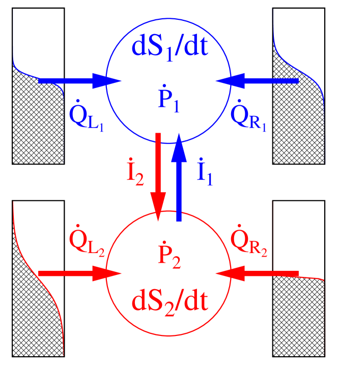
Figure 1: Sketch of a junction which consists of two sub-systems, each coupled to its own baths. Entropy change $dS_{i}/dt$ in subsystem $i$ is caused by heat fluxes $\dot{Q}_{L_{i}}$ and $\dot{Q}_{R_{i}}$, entropy production rate $\dot{P}_{i}$, and information flow $\dot{I}_{i}$.

II Thermodynamics: Green’s functions formulation

We consider a junction which consists of system $S$ strongly coupled to set of baths $\{B\}$. The system and the couplings are subjected to time-dependent driving. Hamiltonian of the model is (here and below $e=k_{B}=\hbar=1$)

$$\hat{H}(t)=\hat{H}_{S}(t)+\sum_{B}\bigg{(}\hat{H}_{B}+\hat{V}_{SB}(t)\bigg{)}$$ (1)

Before system-bath coupling is established at time $t_{0}$, baths are assumed to be in thermal equilibrium characterized by temperature $\beta_{B}=1/T_{B}$ and chemical potential $\mu_{B}$.

System-bath approach to thermodynamics introduced in Ref. Esposito et al., 2010 defines von Neumann expression as the system entropy

$$S(t)\equiv-\mbox{Tr}_{S}\big{[}\hat{\rho}_{S}(t)\,\log\hat{\rho}_{S}(t)\big{]}$$ (2)

Here, $\hat{\rho}(t)$ is the density operator of the universe (system plus baths) and $\hat{\rho}_{S}(t)\equiv\mbox{Tr}_{\{B\}}\big{[}\hat{\rho}(t)\big{]}$. Considering the system and baths initially in the product state $\hat{\rho}(t_{0})=\hat{\rho}_{S}(t_{0})\otimes_{B}\hat{\rho}_{B}^{eq}$, this leads to integral version of the second law in the form Esposito et al. (2010)

$$\Delta S(t)=\sum_{B}\beta_{B}\,Q_{B}(t)+\Delta P(t)$$ (3)

where

$$\begin{split}Q_{B}(t)&\equiv-\mbox{Tr}\big{[}\hat{H}_{B}\,\hat{\rho}(t)\big{]}+\mbox{Tr}\big{[}\hat{H}_{B}\,\hat{\rho}(t_{0})\big{]}\\ \Delta P(t)&\equiv D\big{[}\hat{\rho}(t)||\hat{\rho}_{S}(t)\otimes_{B}\hat{\rho}_{B}^{eq}\big{]}\end{split}$$ (4)

are the heat transferred from bath B into the system and entropy production during time $t-t_{0}$. Here, $D[\hat{\rho}_{1}||\hat{\rho}_{2}]=\mbox{Tr}[\hat{\rho}_{1}\log\hat{\rho}_{1}]-\mbox{Tr}[\hat{\rho}_{1}\log\hat{\rho}_{2}]$ is the quantum relative entropy.

Below, starting from (2) and using NEGF techniques we introduce expressions for thermodynamic characteristics (entropy, entropy production, heat and information fluxes) in terms of single-particle Green’s functions. These expressions are defined in the system subspace only and are suitable for actual calculations. Note that expression for heat in (4) is consistent with definitions of particle and energy fluxes accepted in quantum transport considerations. Also, the system-bath approach (2)-(4) does not introduce artificial additions to the physical system. Thus, thermodynamic formulation is consistent with dynamic (quantum transport) description. Note also that while thermodynamic formulation of Ref. Esposito et al., 2010 strict in assumption of initial product state, Green’s function based analysis in principle allows to relax this restriction by shifting consideration from the Keldysh to Konstantinov-Perel contour Konstantinov and Perel (1961); Wagner (1991). First, we utilize standard NEGF Haug and Jauho (2008); Balzer and Bonitz (2013); Stefanucci and van Leeuwen (2013) and consider non-interacting system. After that, we use the Hubbard NEGF Chen et al. (2017); Miwa et al. (2017); Bergmann and Galperin (2019) to generalize the consideration to interacting systems.

Exact formulations of the second law of thermodynamics in the form of energy resolved partial Clausius, Eq.(8), and local Clausius, Eq. (17), expressions together with equations for the energy resolved entropy, heat, entropy production and information fluxes, Eqs. (9), (18), (19), (27), (28), and (30), are the main results of our consideration.

II.1 Non-interacting system

First, we consider an open non-interacting Fermi system described by the Hamiltonian (1) with

$$\begin{split}\hat{H}_{S}(t)&=\sum_{i,j\in S}H^{S}_{ij}(t)\,\hat{d}_{i}^{\dagger}\hat{d}_{j},\qquad\hat{H}_{B}=\sum_{k\in B}\varepsilon_{k}\hat{c}_{k}^{\dagger}\hat{c}_{k}\\ \hat{V}_{SB}(t)&=\sum_{i\in S}\sum_{k\in B}\bigg{(}V_{ik}(t)\,\hat{d}_{i}^{\dagger}\hat{c}_{k}+V_{ki}(t)\,\hat{c}_{k}^{\dagger}\hat{d}_{i}\bigg{)}\end{split}$$ (5)

Here, $\hat{d}_{i}^{\dagger}$ ($\hat{d}_{i}$) and $\hat{c}_{k}^{\dagger}$ ($\hat{c}_{k}$) creates (annihilates) electron in orbital $i$ of the system and state $k$ of the bath $B$, respectively.

For the non-interacting system (5) entropy (2) is Sharma and Rabani (2015); Bergmann and Galperin (2020)

$$\begin{split}S(t)=&-\mbox{Tr}_{S}\bigg{[}-i\mathbf{G}^{<}(t,t)\,\ln\big{(}-i\mathbf{G}^{<}(t,t)\big{)}\bigg{]}\\ &-\mbox{Tr}_{S}\bigg{[}i\mathbf{G}^{>}(t,t)\,\ln\big{(}i\mathbf{G}^{>}(t,t)\big{)}\bigg{]}\end{split}$$ (6)

where $\mathbf{G}^{\gtrless}(t,t)$ are matrices in the system subspace representing greater/lesser projections of the single-particle Green’s function defined on the Keldysh contour as Haug and Jauho (2008); Balzer and Bonitz (2013); Stefanucci and van Leeuwen (2013)

$$G_{ij}(\tau,\tau^{\prime})\equiv-i\langle T_{c}\,\hat{d}_{i}(\tau)\,\hat{d}_{j}^{\dagger}(\tau^{\prime})\rangle$$ (7)

Here, $T_{c}$ is the contour ordering operator, $\tau_{1,2}$ are the contour variables, operators in the expression are in the Heisenberg picture, and $\langle\ldots\rangle=\mbox{Tr}[\ldots\hat{\rho}(t_{0})]$.

Using (6) and Dyson equation for (7) leads to differential analog of the second law (3) in the form of energy-resolved partial Clausius relation (see Appendix A for details)

$$\frac{d}{dt}S_{B}(t;E)=\beta_{B}\,\dot{Q}_{B}(t;E)+\dot{P}_{B}(t;E)$$ (8)

where

$$\frac{d}{dt}S_{B}(t;E)=\mbox{Tr}_{S}\bigg{[}\mathbf{i}^{B}(t;E)\,\ln\frac{i\mathbf{G}^{>}(t,t)}{-i\mathbf{G}^{<}(t,t)}\bigg{]}$$ (9)

$$\dot{Q}_{B}(t;E)=(E-\mu_{B})\,\mbox{Tr}_{S}\big{[}\mathbf{i}^{B}(t;E)\big{]}$$

$$\dot{P}_{B}(t;E)=\mbox{Tr}_{S}\bigg{[}\mathbf{i}^{B}(t;E)\ln\frac{i\mathbf{G}^{>}(t,t)\,f_{B}(E)}{-i\mathbf{G}^{<}(t,t)\,[1-f_{B}(E)]}\bigg{]}$$

are the bath and energy resolved entropy, heat and entropy production fluxes, and where

$$i^{B}_{ij}(t;E)\equiv\sum_{n\in S}\int_{t_{0}}^{t}ds\,$$ (10)

$$\bigg{(}\big{[}\sigma^{B\,<}_{in}(t,s;E)\,G^{>}_{nj}(s,t)-\sigma^{B\,>}_{in}(t,s;E)\,G^{<}_{nj}(s,t)\big{]}e^{iE(s-t)}$$

$$+\big{[}G^{>}_{in}(t,s)\,\sigma^{B\,<}_{nj}(s,t;E)-G^{<}_{in}(t,s)\,\sigma^{B\,>}_{nj}(s,t;E)\big{]}e^{iE(t-s)}\bigg{)}$$

is the matrix of energy-resolved particle flux at interface $S-B$. Here, $E$ is resolution in the energy of bath states,

$$\begin{split}\sigma^{B\,<}_{i_{1}i_{2}}(t_{1},t_{2};E)&\equiv i\,\gamma^{B}_{i_{1}i_{2}}(t_{1},t_{2};E)\,f_{B}(E)\\ \sigma^{B\,>}_{i_{1}i_{2}}(t_{1},t_{2};E)&\equiv-i\,\gamma^{B}_{i_{1}i_{2}}(t_{1},t_{2};E)\,\big{[}1-f_{B}(E)\big{]}\end{split}$$ (11)

are the lesser and greater projections of the self-energy due to coupling to bath $B$, $f_{B}(E)$ is the Fermi-Dirac thermal distribution, and Jauho et al. (1994)

$$\gamma^{B}_{i_{1}i_{2}}(t_{1},t_{2};E)=2\pi\sum_{k\in B}V_{i_{1}k}(t_{1})\,V_{ki_{2}}(t_{2})\,\delta(E-\varepsilon_{k})$$ (12)

is the energy-resolved dissipation matrix at interface $S-B$.

Expressions (9) introduce energy resolved fluxes of entropy, heat and entropy production. Corresponding total fluxes are obtained by summing over baths and integrating over energy

$$\begin{split}\frac{d}{dt}S(t)&=\sum_{B}\int\frac{dE}{2\pi}\,\frac{d}{dt}S_{B}(t;E)\\ \dot{Q}_{B}(t)&=\int\frac{dE}{2\pi}\,\dot{Q}_{B}(t;E)\\ \dot{P}(t)&=\sum_{B}\int\frac{dE}{2\pi}\,\dot{P}_{B}(t;E)\end{split}$$ (13)

That is, in noninteracting systems the fluxes are exactly additive in terms of bath contributions (below we show that the same is true in presence of interactions). Thus, non-Markov character of Green’s function formulation alleviates non-additivity problems of quantum master equation considerations Chan et al. (2014); Giusteri et al. (2017); Mitchison and Plenio (2018); Friedman et al. (2018).

Additive form of fluxes, Eq.(13), also indicates that for system which consists of several coupled parts,

$$\hat{H}_{S}(t)=\sum_{p=1}^{N_{p}}\hat{H}_{S}^{(p)}(t)+\sum_{p_{1}<p_{2}}^{N_{p}}\hat{H}_{S}^{(p_{1}p_{2})}(t),$$ (14)

such that each part $p$ is connected to its own group of baths $\{B_{p}\}$, one can use expressions for entropy of part $p$,

$$S_{p}(t)=-\mbox{Tr}_{p}\big{[}\hat{\rho}_{p}(t)\,\ln\hat{\rho}_{p}(t)\big{]},$$ (15)

and for multipartite mutual information,

$$I_{1,\ldots,N_{p}}(t)=\sum_{p=1}^{N_{p}}S_{p}(t)-S(t),$$ (16)

to derive energy resolved version of the local Clausius expression (see Appendix A for details)

$$\frac{d}{dt}S_{p}(t;E)=\sum_{B_{p}}\bigg{(}\beta_{B_{p}}\,\dot{Q}_{B_{p}}(t;E)+\dot{P}_{B_{p}}(t;E)\bigg{)}+\dot{I}_{p}(t;E)$$ (17)

Here,

$$\begin{split}&\frac{d}{dt}S_{p}(t;E)=\sum_{B_{p}}\mbox{Tr}_{p}\bigg{[}\mathbf{i}_{p}^{B_{p}}(t;E)\,\ln\frac{i\mathbf{G}_{p}^{>}(t,t)}{-i\mathbf{G}_{p}^{<}(t,t)}\bigg{]}+\\ &2\pi\delta(E)\,\mbox{Tr}_{p}\bigg{[}\big{[}\mathbf{G}^{<}(t,t),\mathbf{H}^{(S)}(t)\big{]}_{p}\,\ln\frac{i\mathbf{G}_{p}^{>}(t,t)}{-i\mathbf{G}_{p}^{<}(t,t)}\bigg{]}\end{split}$$ (18)

and

$$\begin{split}\dot{I}_{p}(t;E)&\equiv\frac{d}{dt}S_{p}(t;E)-\sum_{B_{p}}\frac{d}{dt}S_{B_{p}}(t;E)\\ &=\dot{I}_{p}^{reg}(t;E)+\dot{I}_{p}^{\delta}(t;E)\\ \dot{I}_{p}^{reg}(t;E)&\equiv\sum_{B_{p}}\bigg{(}\mbox{Tr}_{p}\bigg{[}\mathbf{i}_{p}^{B_{p}}(t;E)\,\ln\frac{i\mathbf{G}_{p}^{>}(t,t)}{-i\mathbf{G}_{p}^{<}(t,t)}\bigg{]}\\ &\qquad\,\,-\mbox{Tr}_{S}\bigg{[}\mathbf{i}^{B_{p}}(t;E)\,\ln\frac{i\mathbf{G}^{>}(t,t)}{-i\mathbf{G}^{<}(t,t)}\bigg{]}\bigg{)}\\ \dot{I}_{p}^{\delta}(t;E)&\equiv 2\pi\delta(E)\times\\ &\mbox{Tr}_{p}\bigg{[}\big{[}\mathbf{G}^{<}(t,t),\mathbf{H}^{(S)}(t)\big{]}_{p}\,\ln\frac{i\mathbf{G}_{p}^{>}(t,t)}{-i\mathbf{G}_{p}^{<}(t,t)}\bigg{]}\end{split}$$ (19)

are the part $p$ entropy and information fluxes, respectively. Subscript $p$ in $\big{[}\mathbf{G}^{<}(t,t),\mathbf{H}^{(S)}(t)\big{]}_{p}$, $\mathbf{G}_{p}^{\gtrless}(t,t)$, and $\mathbf{i}_{p}^{B_{p}}(t;E)$ in (18) and (19) indicates matrices in the subspace $p$ of $S$.

II.2 Interacting system

We now turn to interacting systems. In the basis $\{\lvert S\rangle\}$ of many-body states of an isolated system contributions to the Hamiltonian (1) are

$$\hat{H}_{S}(t) =\sum_{S_{1},S_{2}\in S}H^{S}_{S_{1}S_{2}}(t)\hat{X}_{S_{1}S_{2}}$$

$$\hat{H}_{B} =\sum_{k\in B}\varepsilon_{k}\hat{c}_{k}^{\dagger}\hat{c}_{k}$$ (20)

$$\hat{V}_{SB}(t) =\sum_{S_{1},S_{2}\in S}\sum_{k\in B}\bigg{(}V_{(S_{1}S_{2})k}(t)\,\hat{X}_{S_{1}S_{2}}^{\dagger}\hat{c}_{k}+H.c.\bigg{)}$$

Here, $\hat{X}_{S_{1}S_{2}}\equiv\lvert S_{1}\rangle\langle S_{2}\rvert$ is the Hubbard operator. Note that while focus of our consideration is on Fermi baths, generalization to Bose case is straightforward.

Entropy of the system, Eq. (2), is defined by the system density operator. Its representation in the basis of the system many-body states is

$$\big{[}\rho_{S}(t)\big{]}_{S_{1}S_{2}}=\langle\hat{X}_{S_{2}S_{1}}(t)\rangle$$ (21)

Exact equation of motion (EOM) for the system density matrix is (see Appendix B for details)

$$\begin{split}&\frac{d}{dt}\langle\hat{X}_{S_{2}S_{1}}(t)\rangle=-i\big{[}\mathbf{H}^{(S)}(t),\mathbf{\rho}_{S}(t)\big{]}_{S_{1}S_{2}}\\ &+\sum_{B}\int\frac{dE}{2\pi}\,I^{B}_{S_{1}S_{2}}(t;E)\end{split}$$ (22)

where

$$I^{B}_{S_{1}S_{2}}(t;E)\equiv\sum_{S_{3},S_{4},S_{5}\in S}\int_{-\infty}^{t}ds$$ (23)

$$\bigg{(}\ \Sigma^{B\,<}_{(S_{3}S_{1})(S_{4}S_{5})}(t,s;E)\,e^{iE(s-t)}\,\mathcal{G}^{>}_{(S_{4}S_{5})(S_{3}S_{2})}(s,t)$$

$$-\Sigma^{B\,>}_{(S_{3}S_{1})(S_{4}S_{5})}(t,s;E)\,e^{iE(s-t)}\,\mathcal{G}^{<}_{(S_{4}S_{5})(S_{3}S_{2})}(s,t)$$

$$-\Sigma^{B\,<}_{(S_{2}S_{3})(S_{4}S_{5})}(t,s;E)\,e^{iE(s-t)}\,\mathcal{G}^{>}_{(S_{4}S_{5})(S_{1}S_{3})}(s,t)$$

$$+\Sigma^{B\,>}_{(S_{2}S_{3})(S_{4}S_{5})}(t,s;E)\,e^{iE(s-t)}\,\mathcal{G}^{<}_{(S_{4}S_{5})(S_{1}S_{3})}(s,t)$$

$$+\mathcal{G}^{>}_{(S_{3}S_{1})(S_{4}S_{5})}(t,s)\,e^{iE(t-s)}\,\Sigma^{B\,<}_{(S_{4}S_{5})(S_{3}S_{2})}(s,t;E)$$

$$-\mathcal{G}^{<}_{(S_{3}S_{1})(S_{4}S_{5})}(t,s)\,e^{iE(t-s)}\,\Sigma^{B\,>}_{(S_{4}S_{5})(S_{3}S_{2})}(s,t;E)$$

$$-\mathcal{G}^{>}_{(S_{2}S_{3})(S_{4}S_{5})}(t,s)\,e^{iE(t-s)}\,\Sigma^{B\,<}_{(S_{4}S_{5})(S_{1}S_{3})}(s,t;E)$$

$$+\mathcal{G}^{<}_{(S_{2}S_{3})(S_{4}S_{5})}(t,s)\,e^{iE(t-s)}\,\Sigma^{B\,>}_{(S_{4}S_{5})(S_{1}S_{3})}(s,t;E)\bigg{)}$$

is the matrix of energy resolved probability flux at interface $S-B$,

$$\begin{split}\Sigma^{B\,<}_{(S_{1}S_{3})(S_{2}S_{4})}(t_{1},t_{2};E)&\equiv i\,\Gamma^{B}_{(S_{1}S_{3})(S_{2}S_{4})}(t_{1},t_{2};E)\,f_{B}(E)\\ \Sigma^{B\,>}_{(S_{1}S_{3})(S_{2}S_{4})}(t_{1},t_{2};E)&\equiv-i\,\Gamma^{B}_{(S_{1}S_{3})(S_{2}S_{4})}(t_{1},t_{2};E)\,\\ &\qquad\qquad\times[1-f_{B}(E)]\end{split}$$ (24)

are the lesser and greater projections fo the self-energy due to coupling to bath $B$, $f_{B}(E)$ is the Fermi-Dirac thermal distribution, and

$$\begin{split}&\Gamma^{B}_{(S_{1}S_{3})(S_{2}S_{4})}(t_{1},t_{2};E)\equiv\\ &\qquad 2\pi\sum_{k\in B}V_{(S_{1}S_{3})k}(t_{1})\,V_{k(S_{2}S_{4})}(t_{2})\,\delta(E-\varepsilon_{k})\end{split}$$ (25)

is the energy-resolved dissipation matrix. $\mathcal{G}^{\gtrless}_{(S_{1}S_{3})(S_{2}S_{4})}(t_{1},t_{2})$ are greater/lesser projections of the Hubbard Green’s function defined on the Keldysh contour as Chen et al. (2017); Miwa et al. (2017); Bergmann and Galperin (2019)

$$\mathcal{G}_{(S_{1}S_{3})(S_{2}S_{4})}(\tau_{1},\tau_{2})\equiv-i\big{\langle}T_{c}\,\hat{X}_{S_{1}S_{3}}(\tau_{1})\hat{X}_{S_{2}S_{4}}^{\dagger}(\tau_{2})\,\big{\rangle}$$ (26)

EOM (22) leads to expression for second law in the form of energy-resolved version of the partial Clausius relation (8) with entropy, heat and entropy production fluxes given by (see Appendix C for derivation)

$$\frac{d}{dt}S_{B}(t;E)=-\mbox{Tr}_{S}\bigg{[}\mathbf{I}^{B}(t;E)\,\ln\mathbf{\rho}_{S}(t)\bigg{]}$$ (27)

$$\dot{Q}_{B}(t;E)=(E-\mu_{B})\mbox{Tr}_{S}\big{[}\mathbf{N}\,\mathbf{I}^{B}(t;E)\big{]}$$

$$\dot{P}_{B}(t;E)=-\mbox{Tr}_{S}\bigg{[}\mathbf{I}^{B}(t;E)\bigg{(}\ln\mathbf{\rho}_{S}(t)-\mathbf{N}\ln\frac{f_{B}(E)}{1-f_{B}(E)}\bigg{)}\bigg{]}$$

Here, $\mathbf{N}$ is matrix representing the system number operator in the basis of many-body states $\{\lvert S\rangle\}$, its elements $N_{S_{1}S_{2}}\equiv\langle S_{1}\rvert\hat{N}\lvert S_{2}\rangle=\delta_{N_{S_{1}},N_{S_{2}}}\,N_{S_{1}}$ yield information on number of electrons $N_{S}$ in state $\lvert S\rangle$. As previously, total fluxes are given by integrating over energy and summing over baths, Eq.(13).

Finally, for the multipartite system (14) one can derive energy-resolved local Clausius expression (17). Derivation follows the same steps as in the noninteracting case considered in Appendix A. The only new feature is connection between probability and particle/energy fluxes as discussed in Appendix C. Similar to noninteracting case, Eq.(18), consideration of part of the system results in non-zero contribution from the first term in the right of (22) to the entropy flow

$$\begin{split}&\frac{d}{dt}S_{p}(t;E)=-\sum_{B_{p}}\mbox{Tr}_{p}\bigg{[}\mathbf{I}_{p}^{B_{p}}(t;E)\,\ln\mathbf{\rho}_{p}(t)\bigg{]}\\ &\qquad+2\pi i\delta(E)\,\mbox{Tr}_{p}\bigg{[}\big{[}\mathbf{H}^{(S)}(t),\mathbf{\rho}_{S}(t)\big{]}_{p}\,\ln\mathbf{\rho}_{p}(t)\bigg{]}\end{split}$$ (28)

Here,

$$\begin{split}&\hat{\rho}_{p}(t)\equiv\mbox{Tr}_{S\setminus p}\big{[}\hat{\rho}_{S}(t)\big{]},\quad\mathbf{I}_{p}^{B_{p}}(t;E)\equiv\mbox{Tr}_{S\setminus p}\big{[}\mathbf{I}^{B_{p}}(t;E)\big{]},\\ &\big{[}\mathbf{H}^{(S)}(t),\mathbf{\rho}_{S}(t)\big{]}_{p}\equiv\mbox{Tr}_{S\setminus p}\bigg{[}\big{[}\mathbf{H}^{(S)}(t),\mathbf{\rho}_{S}(t)\big{]}\bigg{]}.\end{split}$$ (29)

Using (8), (27) and (28) in energy resolved analog of (16) (see Eq. (48) in Appendix A), leads to the energy resolved local Clausius expression (17) with information flux given by

$$\begin{split}\dot{I}_{p}(t;E)&=\dot{I}_{p}^{reg}(t;E)+\dot{I}_{p}^{\delta}(t;E)\\ \dot{I}_{p}^{reg}(t;E)&\equiv\sum_{B_{p}}\bigg{(}\mbox{Tr}_{S}\bigg{[}\mathbf{I}^{B_{p}}(t;E)\,\ln\mathbf{\rho}_{S}(t)\bigg{]}\\ &\qquad\,\,-\mbox{Tr}_{p}\bigg{[}\mathbf{I}_{p}^{B_{p}}(t;E)\,\ln\mathbf{\rho}_{p}(t)\bigg{]}\bigg{)}\\ \dot{I}_{p}^{\delta}(t;E)&\equiv 2\pi i\delta(E)\times\\ &\mbox{Tr}_{p}\bigg{[}\big{[}\mathbf{H}^{(S)}(t),\mathbf{\rho}_{S}(t)\big{]}_{p}\,\ln\mathbf{\rho}_{p}(t)\bigg{]}\end{split}$$ (30)

III Numerical illustrations

Here we illustrate our derivations with simulations performed in generic junction model sketched in Fig. 1. Fermi energy $E_{F}$ in each bath is taken as zero, and bias $V_{i}$ between left and right sides is applied symmetrically, $\mu_{L_{i}}=E_{F}+V_{i}/2$ and $\mu_{R_{i}}=E_{F}-V_{i}/2$ ($i=1,2$). Simulations are performed at steady state.

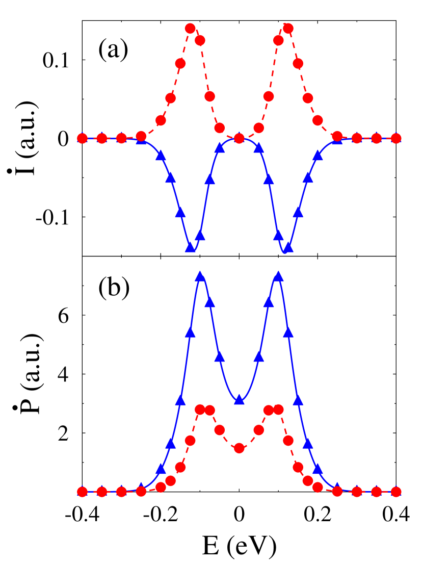
Figure 2: Junction of Fig. 1 with $S$ represented by two-level system. Shown are steady state energy resolved (a) information flow $\dot{I}$, Eq. (19), and (b) entropy production $\dot{P}$, Eq. (9). Characteristics of parts $S_{1}$ and $S_{2}$ are shown with solid (blue) and dashed (red) lines, respectively. Triangles (blue) and circles (red) present information flow and entropy production evaluated using formulation for interacting systems, Eqs. (30) and (27). See text for parameters.

First, we consider two-level system as an example for noninteracting $S$. Hamiltonian of the system is given in Eq.(14) with

$$\begin{split}&\hat{H}_{S}^{(i)}=\varepsilon_{i}\hat{d}_{i}^{\dagger}\hat{d}_{i}\quad(i=1,2)\\ &\hat{H}_{S}^{(12)}=t_{12}\big{(}\hat{d}_{1}^{\dagger}\hat{d}_{2}+\hat{d}_{2}^{\dagger}\hat{d}_{1}\big{)}\end{split}$$ (31)

Here, $\hat{d}_{i}^{\dagger}$ ($\hat{d}_{i}$) creates (annihilates) electron in level $\varepsilon_{i}$ of subsystem $S_{i}$.

Figure 2 shows results of the simulation. Parameters are $T=300$ K, $\varepsilon_{1}=\varepsilon_{2}=0$, $t_{12}=0.1$ eV, $\gamma^{B}_{ij}=\delta_{i,j}\,0.05$ eV, $V_{1}=0.4$ eV and $V_{2}=-0.2$ eV. Simulation was performed on energy grid spanning range from $-10$ to $10$ eV with step $0.001$ eV. Panel (a) shows information flow from $S_{1}$ and into $S_{2}$, which is natural consequence of $V_{1}>\lvert V_{2}\rvert$. Because of steady-state $\dot{I}_{1}=-\dot{I}_{2}$. Entropy production is presented in panel (b). The simulations were performed utilizing non-interacting (lines) and interacting (markers) methodology. Fig. 2 shows close correspondence between NEGF and Hubbard NEGF results.

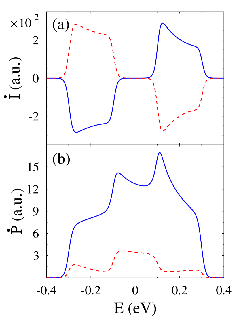
Figure 3: Junction of Fig. 1 with $S$ represented by quantum dot in the limit of strong Coulomb repulsion. Subsystem $S_{1}$ represents spin up and $S_{2}$ represents spin down levels. Shown are steady state energy resolved (a) information flow $\dot{I}$, Eq. (30), and (b) entropy production $\dot{P}$, Eq. (27). Characteristics of parts $S_{1}$ and $S_{2}$ are shown with solid (blue) and dashed (red) lines, respectively. See text for parameters.

We now turn to consider interacting system. As a toy model we take quantum dot junction in the regime of strong Coulomb repulsion. Subsystems $S_{1}$ and $S_{2}$ represent spin up and spin down levels of the system. The dot is subjected coupling to external spin degree of freedom (e.g. magnetic adatom) induces spin-flip processes which we model by effective electron transfer matrix element between the two levels. Hamiltonian has a form (14) with

$$\begin{split}&\sum_{i=1}^{2}\hat{H}_{S}^{(i)}=\sum_{\sigma=\uparrow,\downarrow}\varepsilon_{\sigma}\hat{d}_{\sigma}^{\dagger}\hat{d}_{\sigma}+U\hat{n}_{\uparrow}\hat{n}_{\downarrow}\\ &\hat{H}_{S}^{(12)}=t_{12}\left(\hat{d}_{\uparrow}^{\dagger}\hat{d}_{\downarrow}+H.c.\right)\end{split}$$ (32)

Here, $\hat{d}_{\sigma}^{\dagger}$ ($\hat{d}_{\sigma}$) creates (annihilates) electron of spin $\sigma$ in level $\varepsilon_{\sigma}$, $\hat{n}_{\sigma}\equiv\hat{d}_{\sigma}^{\dagger}\hat{d}_{\sigma}$. We consider strong Coulomb repulsion, $U\to\infty$, in the parameter regime where Kondo feature is detectable. Simulations were performed utilizing equation of motion approach to the Hubbard Green’s functions within a method presented in Ref. Ochoa et al., 2014. We note that such consideration yields Kondo feature only qualitatively, which is enough for illustration purposes. More elaborate considerations should employ more advanced decoupling scheme of Ref. Lacroix, 1981 or rely on numerically exact techniques.

Figure 3 shows results of the simulation. Parameters are $T=100$ K, $\varepsilon_{\uparrow}=\varepsilon_{\downarrow}=-2$ eV, $t_{12}=0.5$ eV, $\gamma^{B}_{ij}=\delta_{i,j}\,0.5$ eV, $V_{\uparrow}=0.6$ eV and $V_{\downarrow}=0.2$ eV. Simulation was performed on energy grid spanning range from $-10$ to $10$ eV with step $0.001$ eV. Information flow (panel a), entropy production is presented in panel (b). Note that entropy production for $S_{1}$ demonstrate Kondo features near chemical potentials of the opposite spin ($E=\pm 0.1$ eV). The feature at $E=0.1$ eV is also observed in the information flow. Note also that contrary to the noninteracting case, where information flow is always from $S_{1}$ into $S_{2}$, interacting model yields more structured energy profile. This example indicates potential importance of strong correlations in thermodynamic properties of systems strongly coupled to their baths.

IV Conclusion

Starting from von Neumann expression with reduced (system) density matrix as definition of thermodynamic entropy for a system strongly coupled to its baths, we formulate the second law of thermodynamics in the form of bath and energy resolved partial and local Clausius relations. The derivation yields expressions for entropy, heat, and information flows and for entropy production rate formulated in terms of system variables only. This makes the expressions suitable for actual calculations of the thermodynamic characteristics of open nanoscale molecular devices.

The expressions are derived using the standard NEGF for noninteracting and Hubbard NEGF for interacting systems. Utilization of Green’s function techniques allows to generalize Markov weak coupling (second order in system-baths) consideration of Ref. Ptaszyński and Esposito (2019) to strongly coupled case of non-Markov system dynamics. In particular, we utilize exact equation of motion for the reduced (system) density matrix in terms of Green’s functions, introduce energy resolution of the thermodynamic flows, and show that Green’s function analysis allows to alleviate non-separability problems of density matrix considerations and thus to introduce exact general form of information flow. Expressions for thermodynamic characteristics reduce to known expected limiting forms in weak coupling or steady-state situations. We stress that while theoretical consideration in the manuscript focuses on Fermi baths and charge flux between the system and baths, generalization to incorporate Bose degrees of freedom and energy flux is straightforward within the interacting (Hubbard NEGF) formulation.

Theoretical derivations are illustrated with numerical results for a junction which consists fo two sub-systems each coupled its own pair of baths (Fig. 1). Generic models of the two-level system and quantum dot with spin-flip processes are used as illustrations for noninteracting and interacting system, respectively. Energy resolved thermodynamic characteristics of the interacting system are shown to demonstrate strongly correlated features (Kondo), which in principle can be detected in corresponding flows similar to conductance measurements.

Appendix A Derivation of energy resolved partial and local Clausius expression for noninteracting system

For noninteracting systems (i.e. systems described by quadratic Hamiltonian), the Wick’s theorem holds for any part of the universe (system plus baths). This means that corresponding many-body density operator for any part of the system has Gaussian form. Thus, path integral formulation yields for the local density matrix Bergmann and Galperin (2020)

$$\rho_{A}(t)=\mbox{det}\big{[}i\mathbf{G}_{A}^{>}(t,t)\big{]}\frac{-i\mathbf{G}_{A}^{<}(t,t)}{i\mathbf{G}_{A}^{>}(t,t)}$$ (33)

Here, $A$ can be any part of the universe. Below we consider system ($A=S$) or its part ($A=p$), and assume that each part $p$ of the system is coupled to its own set of baths $\{B_{p}\}$.

Assuming von Neumann expression for entropy of the part $A$, Eq.(33) leads to

$$\begin{split}S_{A}(t)=&-\mbox{Tr}_{A}\big{[}\rho_{A}(t)\,\ln\rho_{A}(t)\big{]}\\ =&-\mbox{Tr}_{A}\big{[}-i\mathbf{G}_{A}^{<}(t,t)\,\ln\big{(}-i\mathbf{G}_{A}^{<}(t,t)\big{)}\big{]}\\ &-\mbox{Tr}_{A}\big{[}i\mathbf{G}_{A}^{>}(t,t)\,\ln\big{(}i\mathbf{G}_{A}^{>}(t,t)\big{)}\big{]}\end{split}$$ (34)

Here, $\mathbf{G}_{A}^{\gtrless}(t,t)$ is the greater/lesser projection of the single-particle Green’s function for the system, $\mathbf{G}^{\gtrless}(t,t)$ ($A=S$), or its part, $\mathbf{G}^{\gtrless}_{p}(t,t)$ ($A=p$). Taking time derivative of (34) leads to expression for entropy flux

$$\frac{d}{dt}S_{A}(t)=\mbox{Tr}_{A}\bigg{[}\bigg{(}-i\frac{d}{dt}\mathbf{G}_{A}^{<}(t,t)\bigg{)}\,\ln\frac{i\mathbf{G}_{A}^{>}(t,t)}{-i\mathbf{G}_{A}^{<}(t,t)}\bigg{]}$$ (35)

Dyson equation for the lesser projection of the single particle Green’s function is

$$-i\frac{d}{dt}\big{(}G_{A}^{<}(t,t)\big{)}_{ij}=\big{[}\mathbf{G}^{<}(t,t),\mathbf{H}^{(S)}(t)\big{]}_{ij}$$ (36)

$$+\sum_{n\in S}\int_{t_{0}}^{t}ds\,\bigg{(}G^{r}_{in}(t,s)\,\sigma^{<}_{nj}(s,t)+G^{<}_{in}(t,s)\,\sigma^{a}_{nj}(s,t)$$

$$\qquad\qquad\quad-\sigma^{r}_{in}(t,s)\,G^{<}_{nj}(s,t)-\sigma^{<}_{in}(t,s)\,G^{a}_{nj}(s,t)\bigg{)}$$

Here, $i,j\in A$, $</r/a$ is the lesser/retarded/advanced projection, $G$ is defined in (7), and for noninteracting system self-energy $\sigma$ is

$$\begin{split}\sigma_{ij}(\tau,\tau^{\prime})&=\sum_{B}\sigma^{B}_{ij}(\tau,\tau^{\prime})\\ \sigma^{B}_{ij}(\tau,\tau^{\prime})&\equiv\sum_{k\in B}V_{ik}(t)\,g_{k}(\tau,\tau^{\prime})\,V_{kj}(t^{\prime})\end{split}$$ (37)

where $g_{k}(\tau,\tau^{\prime})$ is single-particle Green’s function of free electron in state $k$ of the bath $B$. Substituting (37) into (36) and using

$$\begin{split}\mathbf{G}^{r}(t,t^{\prime})&=\theta(t-t^{\prime})\big{(}\mathbf{G}^{>}(t,t^{\prime})-\mathbf{G}^{<}(t,t^{\prime})\big{)}\\ \mathbf{G}^{a}(t,t^{\prime})&=\theta(t^{\prime}-t)\big{(}\mathbf{G}^{<}(t,t^{\prime})-\mathbf{G}^{>}(t,t^{\prime})\big{)}\end{split}$$ (38)

and similar expressions for $\sigma$ leads to

$$-i\frac{d}{dt}\big{(}G_{A}^{<}(t,t)\big{)}_{ij}=\big{[}\mathbf{G}^{<}(t,t),\mathbf{H}^{(S)}(t)\big{]}_{ij}$$ (39)

$$+\sum_{B}\sum_{n\in S}\int_{t_{0}}^{t}ds\,\big{(}\sigma^{B\,<}_{in}(t,s)\,G^{>}_{nj}(s,t)+G^{>}_{in}(t,s)\,\sigma^{B\,<}_{nj}(s,t)$$

$$\qquad\qquad\qquad-\sigma^{B\,>}_{in}(t,s)\,G^{<}_{nj}(s,t)-G^{<}_{in}(t,s)\,\sigma^{B\,>}_{nj}(s,t)\big{)}$$

Using the Jauho-Wingreen-Meir expression for particle flux $I_{B}(t)$ at interface $S-B$ Jauho et al. (1994)

$$\begin{split}&I_{B}(t)=\\ &\int_{t_{0}}^{t}ds\,\mbox{Tr}_{S}\bigg{[}\mathbf{\sigma}^{B\,<}(t,s)\,\mathbf{G}^{>}(s,t)+\mathbf{G}^{>}(t,s)\,\mathbf{\sigma}^{B\,<}(s,t)\\ &\qquad\qquad-\mathbf{\sigma}^{B\,>}(t,s)\,\mathbf{G}^{<}(s,t)-\mathbf{G}^{<}(t,s)\,\mathbf{\sigma}^{B\,>}(s,t)\bigg{]},\end{split}$$ (40)

(37) with

$$\begin{split}g_{k}^{<}(t,t^{\prime})&=in_{k}e^{-i\varepsilon_{k}(t-t^{\prime})}\\ g_{k}^{>}(t,t^{\prime})&=-i[1-n_{k}]e^{-i\varepsilon_{k}(t-t^{\prime})},\end{split}$$ (41)

and

$$\sum_{k\in B}\ldots\equiv\int\frac{dE}{2\pi}\,2\pi\sum_{k\in B}\delta(E-\varepsilon_{k})\ldots$$ (42)

leads to

$$\begin{split}-i\frac{d}{dt}\big{(}G_{A}^{<}(t,t)\big{)}_{ij}&=\big{[}\mathbf{G}^{<}(t,t),\mathbf{H}^{(S)}(t)\big{]}_{ij}\\ &+\sum_{B_{A}}\int\frac{dE}{2\pi}\,i^{B_{A}}_{ij}(t;E)\end{split}$$ (43)

where the matrix of energy-resolved particle flux $\mathbf{i}^{B}(t;E)$ is defined in (10).

Substituting (43) into (35) yields

$$\begin{split}\frac{d}{dt}S_{A}(t)&=\mbox{Tr}_{A}\bigg{[}\big{[}\mathbf{G}^{<}(t,t),\mathbf{H}^{(S)}(t)\big{]}_{A}\,\ln\frac{i\mathbf{G}_{A}^{>}(t,t)}{-i\mathbf{G}_{A}^{<}(t,t)}\bigg{]}\\ &+\sum_{B_{A}}\int\frac{dE}{2\pi}\,\mbox{Tr}_{A}\bigg{[}\mathbf{i}_{A}^{B_{A}}\,\ln\frac{i\mathbf{G}_{A}^{>}(t,t)}{-i\mathbf{G}_{A}^{<}(t,t)}\bigg{]}\end{split}$$ (44)

where subscript $A$ in $\big{[}\mathbf{G}^{<}(t,t),\mathbf{H}^{(S)}(t)\big{]}_{A}$, $\mathbf{G}_{A}^{\gtrless}(t,t)$, and $\mathbf{i}_{A}^{B_{A}}$ indicates sub-matrix with indices in subspace $A$.

Partial Clausius expression, Eq.(8)

We now restrict our consideration to the system ($A=S$). In this case first term in the right side of (44) is identically zero, and we can introduce energy-resolved version of the entropy flux as defined in (9) and (13). Energy resolved version of the partial Clausius inequality (8) follows from

$$\ln\frac{f_{B}(E)}{1-f_{B}(E)}=-\beta_{B}(E-\mu_{B})$$ (45)

and definitions of energy resolved heat and entropy production fluxes given in (9). Note that definition of the heat flux $\dot{Q}_{B}(t)$ is consistent with the standard quantum transport definitions of particle $I_{B}(t)$ and energy $J_{B}(t)$ fluxes

$$\begin{split}\dot{Q}_{B}(t)&\equiv J_{B}(t)-\mu_{B}\,I_{B}(t)\\ J_{B}(t)&\equiv-\frac{d}{dt}\langle\hat{H}_{B}(t)\rangle\\ I_{B}(t)&\equiv-\frac{d}{dt}\sum_{k\in B}\langle\hat{c}_{k}^{\dagger}(t)\hat{c}_{k}(t)\rangle\end{split}$$ (46)

Local Clausius expression, Eq.(17)

Now we restrict our consideration to part $p$ of the system ($A=p$). Part $p$ is assumed to be coupled to its own set of baths $\{B_{p}\}$, so that $\sum_{B}\sum_{n\in S}\ldots$ in the second term in the right of (39) is substituted by $\sum_{B_{p}}\sum_{n\in p}\ldots$. Thus, matrix for energy-resolved particle $i^{B}_{ij}$, Eq. (10), is substituted by similar expression $\big{[}i_{p}^{B_{p}}\big{]}_{ij}$ with $i,j\in p$ and $\sum_{n\in S}\ldots\to\sum_{n\in p}\ldots$

$$\big{[}i_{p}^{B_{p}}\big{]}_{ij}(t;E)\equiv\sum_{n\in p}\int_{t_{0}}^{t}ds\,$$ (47)

$$\bigg{(}\big{[}\sigma^{B_{p}\,<}_{in}(t,s;E)\,G^{>}_{nj}(s,t)-\sigma^{B_{p}\,>}_{in}(t,s;E)\,G^{<}_{nj}(s,t)\big{]}e^{iE(s-t)}$$

$$+\big{[}G^{>}_{in}(t,s)\,\sigma^{B_{p}\,<}_{nj}(s,t;E)-G^{<}_{in}(t,s)\,\sigma^{B_{p}\,>}_{nj}(s,t;E)\big{]}e^{iE(t-s)}\bigg{)}$$

This is the current expression in the second term of (44).

Main difference (when compared with $A=S$) is non-zero contribution from the first term in the right in (44). Thus, energy-resolved expression for bath specific entropy flux of the system, Eq. (9), is substituted with part specific expression, Eq.(18), with additional delta-term in it.

Using (8), (9) and (18) in energy resolved analog of (16),

$$I_{1,\ldots,N_{p}}=\int\frac{dE}{2\pi}\,I_{1,\ldots,N_{p}}(t;E),$$ (48)

leads to separability of the multipartite mutual information into part-specific contributions

$$\begin{split}&\dot{I}_{1,\ldots,N_{p}}(t;E)=\sum_{p}\frac{d}{dt}S_{p}(t;E)\\ &\quad-\sum_{p}\sum_{B_{p}}\bigg{(}\beta_{B_{p}}\dot{Q}_{B_{p}}(t;E)+\dot{P}_{B_{p}}(t;E)\bigg{)}\\ &\quad\equiv\sum_{p}\dot{I}_{p}(t;E)\end{split}$$ (49)

Rearranging terms in the latter expression yields (17) with information flux consisting of regular and delta-type contributions as defined in Eq.(19).

Appendix B Derivation of exact EOM for system density matrix, Eq.(22)

We start with writing Heisenberg EOM for $\hat{X}_{S_{2}S_{1}}(t)$ under dynamics governed by the Hamiltonian (1) and (II.2). Averaging result over an initial density operator leads to

$$\frac{d}{dt}\big{\langle}\hat{X}_{S_{2}S_{1}}(t)\big{\rangle}=$$

$$i\sum_{S_{3}}\big{\langle}H^{(S)}_{S_{3}S_{2}}(t)\,\hat{X}_{S_{3}S_{1}}(t)-H^{(S)}_{S_{1}S_{3}}(t)\,\hat{X}_{S_{2}S_{3}}(t)\big{\rangle}$$

$$+\sum_{B}\sum_{k\in B}\sum_{S_{3}\in S}$$ (50)

$$\bigg{(}\ \ V_{(S_{2}S_{3})\,k}(t)\,\mathcal{G}^{<}_{k\,(S_{1}S_{3})}(t,t)-V_{(S_{3}S_{1})\,k}(t)\,\mathcal{G}^{<}_{k\,(S_{3}S_{2})}(t,t)$$

$$+V_{k\,(S_{3}S_{2})}(t)\,\mathcal{G}^{<}_{(S_{3}S_{1})\,k}(t,t)-V_{k\,(S_{1}S_{3})}(t)\,\mathcal{G}^{<}_{(S_{2}S_{3})\,k}(t,t)\bigg{)}$$

where $\mathcal{G}_{(SS^{\prime})\,k}^{\gtrless}(t,t)$ and $\mathcal{G}^{\gtrless}_{k\,(SS^{\prime})}(t,t)$ are the equal time greater/lesser projections of the Hubbard Green’s functions defined on the contour as

$$\begin{split}\mathcal{G}_{(SS^{\prime})\,k}(\tau,\tau^{\prime})&\equiv-i\big{\langle}T_{c}\,\hat{X}_{SS^{\prime}}(\tau)\,\hat{c}_{k}^{\dagger}(\tau^{\prime})\big{\rangle}\\ \mathcal{G}_{k\,(SS^{\prime})}(\tau,\tau^{\prime})&\equiv-i\big{\langle}T_{c}\,\hat{c}_{k}(\tau)\,\hat{X}_{SS^{\prime}}^{\dagger}(\tau^{\prime})\big{\rangle}\end{split}$$ (51)

Integral forms of the right and left Dyson equations for (51) are

$$\mathcal{G}_{(SS^{\prime})\,k}(\tau,\tau^{\prime})=$$ (52)

$$\sum_{S_{4},S_{5}\in S}\int_{c}d\sigma\,\mathcal{G}_{(SS^{\prime})(S_{4}S_{5})}(\tau,\sigma)\,V_{(S_{4}S_{5})\,k}(s)\,g_{k}(\sigma,\tau^{\prime})$$

$$\mathcal{G}_{k\,(SS^{\prime})}(\tau,\tau^{\prime})=$$

$$\sum_{S_{4},S_{5}\in S}\int_{c}d\sigma\,g_{k}(\tau,\sigma)\,V_{k\,(S_{4}S_{5})}(s)\,\mathcal{G}_{(S_{4}S_{5})(SS^{\prime})}(\sigma,\tau^{\prime})$$

where

$$g_{k}(\tau,\tau^{\prime})\equiv-i\langle T_{c}\,\hat{c}_{k}(\tau)\,\hat{c}_{k}^{\dagger}(\tau^{\prime})\rangle$$ (53)

is the single-particle Green’s function of free electron in state $k$ of contact $B$.

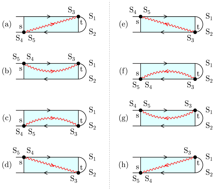
Figure 4: Projections representing terms in Eq. (54). Directed wavy line (red) indicates self-energy, shaded square (cyan) represents evolution accounted for by the Hubbard Green’s function.

Substituting lesser projections of (52) into (B) leads to

$$\frac{d}{dt}\big{\langle}\hat{X}_{S_{2}S_{1}}(t)\big{\rangle}=-i\big{[}\mathbf{H}^{(S)}(t),\mathbf{\rho}_{S}(t)\big{]}_{S_{1}S_{2}}$$ (54)

$$+\sum_{B}\sum_{S_{3},S_{4},S_{5}\in S}\int_{t_{0}}^{t}ds$$

$$\bigg{(}\ \Sigma^{B\,<}_{(S_{3}S_{1})(S_{4}S_{5})}(t,s)\,\mathcal{G}^{>}_{(S_{4}S_{5})(S_{3}S_{2})}(s,t)$$ (a)

$$-\Sigma^{B\,>}_{(S_{3}S_{1})(S_{4}S_{5})}(t,s)\,\mathcal{G}^{<}_{(S_{4}S_{5})(S_{3}S_{2})}(s,t)$$ (b)

$$-\Sigma^{B\,<}_{(S_{2}S_{3})(S_{4}S_{5})}(t,s)\,\mathcal{G}^{>}_{(S_{4}S_{5})(S_{1}S_{3})}(s,t)$$ (c)

$$+\Sigma^{B\,>}_{(S_{2}S_{3})(S_{4}S_{5})}(t,s)\,\mathcal{G}^{<}_{(S_{4}S_{5})(S_{1}S_{3})}(s,t)$$ (d)

$$+\mathcal{G}^{>}_{(S_{3}S_{1})(S_{4}S_{5})}(t,s)\,\Sigma^{B\,<}_{(S_{4}S_{5})(S_{3}S_{2})}(s,t)$$ (e)

$$-\mathcal{G}^{<}_{(S_{3}S_{1})(S_{4}S_{5})}(t,s)\,\Sigma^{B\,>}_{(S_{4}S_{5})(S_{3}S_{2})}(s,t)$$ (f)

$$-\mathcal{G}^{>}_{(S_{2}S_{3})(S_{4}S_{5})}(t,s)\,\Sigma^{B\,<}_{(S_{4}S_{5})(S_{1}S_{3})}(s,t)$$ (g)

$$+\mathcal{G}^{<}_{(S_{2}S_{3})(S_{4}S_{5})}(t,s)\,\Sigma^{B\,>}_{(S_{4}S_{5})(S_{1}S_{3})}(s,t)\bigg{)}$$ (h)

where $\Sigma^{B\,\gtrless}_{(S_{1}S_{2})(S_{3}S_{4})}(t,t^{\prime})$ are the greater/lesser projections of the self-energy due to coupling to contact $B$

$$\begin{split}&\Sigma^{B}_{(S_{1}S_{2})(S_{3}S_{4})}(\tau,\tau^{\prime})\equiv\\ &\quad\sum_{k\in B}V_{(S_{1}S_{2})\,k}(t)\,g_{k}(\tau,\tau^{\prime})\,V_{k\,(S_{3}S_{4})}(t^{\prime})\end{split}$$ (55)

Graphic representation of the projections in (54) is given in Fig. 4. We note in passing that suggestion of Ref. Whitney, 2018 to drop same branch projections (e.g., projections (b), (f), (c) and (g) in second order in system-bath coupling) when building thermodynamic description is inconsistent with assumption of von Neumann form of the system entropy. Note also that connection between exact EOM (54) and approximate quantum master equations for reduced density matrix was discussed in Ref. Bergmann and Galperin, 2019.

Finally, using (41) and (42) in (54) leads to (22).

Appendix C Derivation of partial Clausius expression for interacting system

We start from von Neumann expression for system entropy, Eq. (2), and take time derivative to get entropy flux

$$\frac{d}{dt}S(t)=-\mbox{Tr}_{S}\bigg{[}\frac{d}{dt}\mathbf{\rho}_{S}(t)\,\ln\mathbf{\rho}_{S}(t)\bigg{]}$$ (56)

Using exact EOM for the system density matrix, Eq.(22), and taking into account that first term in the right of (22) gives zero contribution to the trace in (56) and second term in the right of (22) is exactly separable into energy-resolved contributions from different baths leads to

$$\frac{d}{dt}S(t)=\sum_{B}\int\frac{dE}{2\pi}\,\frac{d}{dt}S_{B}(t;E)$$ (57)

where energy-resolved entropy flux $\frac{d}{dt}S_{B}(t;E)$ is defined in (27).

Contrary to noninteracting case, second term in the right of (22) is not directly related to particle flux, rather it is probability flux. Indeed, writing Heisenberg EOM for the current at interface $S-B$, Eq. (46), yields

$$\begin{split}I_{B}(t)&\equiv-\frac{d}{dt}\sum_{k\in B}\big{\langle}\hat{c}_{k}^{\dagger}(t)\hat{c}_{k}(t)\big{\rangle}\\ &=-i\sum_{k\in B}\big{\langle}\big{[}\hat{H}(t),\hat{c}_{k}^{\dagger}(t)\hat{c}_{k}(t)\big{]}\big{\rangle}\\ &=-2\,\mbox{Re}\sum_{S_{1},S_{2}\in S}\sum_{k\in B}V_{(S_{1}S_{2})\,k}(t)\,\mathcal{G}^{<}_{k\,(S_{1}S_{2})}(t,t)\\ &=2\mbox{Re}\sum_{S_{1},S_{2},S_{3},S_{4}\in S}\int_{t_{0}}^{t}ds\,\\ &\bigg{(}\,\,\Sigma^{B\,<}_{(S_{1}S_{2})(S_{3}S_{4})}(t,s)\,\mathcal{G}^{>}_{(S_{3}S_{4})(S_{1}S_{2})}(s,t)\\ &-\Sigma^{B\,>}_{(S_{1}S_{2})(S_{3}S_{4})}(t,s)\,\mathcal{G}^{<}_{(S_{3}S_{4})(S_{1}S_{2})}(s,t)\bigg{)}\end{split}$$ (58)

which is not equivalent to expression in the right of (22).

Connection between probability and particle fluxes is established considering change in particle number of the system caused by coupling to baths

$$\begin{split}\frac{d}{dt}\langle\hat{N}(t)\rangle&=\mbox{Tr}_{S}\bigg{[}\hat{N}\,\frac{d}{dt}\hat{\rho}_{S}(t)\bigg{]}\\ &=\sum_{S_{1}\in S}\sum_{B}\int\frac{dE}{2\pi}\,N_{S_{1}}\,I^{B}_{S_{1}S_{1}}(t;E)\end{split}$$ (59)

where energy resolved probability flux is defined in (23). Thus, energy-resolved particle flux at interface $S-B$ is

$$\sum_{S_{1}\in S}N_{S_{1}}\,I^{B}_{S_{1}S_{1}}(t;E)$$ (60)

Similarly, energy-resolved energy flux at interface $S-B$ is

$$\sum_{S_{1}\in S}E\,N_{S_{1}}\,I^{B}_{S_{1}S_{1}}(t;E)$$ (61)

Expressions (60) and (61) are used in definition of heat flux in (27).

Energy resolved partial Clausius expression (8) for interacting system directly follows from (56) and definitions in (27).

References

• Reddy et al. (2007) P. Reddy, S.-Y. Jang, R. A. Segalman, and A. Majumdar, Science 315, 1568 (2007).
• Lee et al. (2013) W. Lee, K. Kim, W. Jeong, L. A. Zotti, F. Pauly, J. C. Cuevas, and P. Reddy, Nature 498, 209 (2013).
• Kim et al. (2014) Y. Kim, W. Jeong, K. Kim, W. Lee, and P. Reddy, Nature Nanotech. 9, 881 (2014).
• Zotti et al. (2014) L. A. Zotti, M. Bürkle, F. Pauly, W. Lee, K. Kim, W. Jeong, Y. Asai, P. Reddy, and J. C. Cuevas, New J. Phys. 16, 015004 (2014).
• Cui et al. (2017a) L. Cui, R. Miao, C. Jiang, E. Meyhofer, and P. Reddy, J. Chem. Phys. 146, 092201 (2017a).
• Cui et al. (2017b) L. Cui, W. Jeong, S. Hur, M. Matt, J. C. Klöckner, F. Pauly, P. Nielaba, J. C. Cuevas, E. Meyhofer, and P. Reddy, Science 355, 1192 (2017b).
• Cui et al. (2018) L. Cui, R. Miao, K. Wang, D. Thompson, L. A. Zotti, J. C. Cuevas, E. Meyhofer, and P. Reddy, Nature Nanotech. 13, 122 (2018).
• Cui et al. (2019) L. Cui, S. Hur, Z. A. Akbar, J. C. Klöckner, W. Jeong, F. Pauly, S.-Y. Jang, P. Reddy, and E. Meyhofer, Nature 572, 628 (2019).
• Jezouin et al. (2013) S. Jezouin, F. D. Parmentier, A. Anthore, U. Gennser, A. Cavanna, Y. Jin, and F. Pierre, Science 342, 601 (2013).
• Pekola (2015) J. P. Pekola, Nature Phys. 11, 118 (2015).
• Hartman et al. (2018) N. Hartman, C. Olsen, S. Lüscher, M. Samani, S. Fallahi, G. C. Gardner, M. Manfra, and J. Folk, Nature Phys. 14, 1083 (2018).
• Klatzow et al. (2019) J. Klatzow, J. N. Becker, P. M. Ledingham, C. Weinzetl, K. T. Kaczmarek, D. J. Saunders, J. Nunn, I. A. Walmsley, R. Uzdin, and E. Poem, Phys. Rev. Lett. 122, 110601 (2019).
• Esposito et al. (2015a) M. Esposito, M. A. Ochoa, and M. Galperin, Phys. Rev. Lett. 114, 080602 (2015a).
• Esposito et al. (2015b) M. Esposito, M. A. Ochoa, and M. Galperin, Phys. Rev. B 92, 235440 (2015b).
• Uzdin et al. (2016) R. Uzdin, A. Levy, and R. Kosloff, Entropy 18, 124 (2016).
• Katz and Kosloff (2016) G. Katz and R. Kosloff, Entropy 18, 186 (2016).
• Carrega et al. (2016) M. Carrega, P. Solinas, M. Sassetti, and U. Weiss, Phys. Rev. Lett. 116 (2016).
• Strasberg et al. (2016) P. Strasberg, G. Schaller, N. Lambert, and T. Brandes, New J. Phys. 18, 073007 (2016).
• Kato and Tanimura (2016) A. Kato and Y. Tanimura, J. Chem. Phys. 145, 224105 (2016).
• Hsiang and Hu (2018) J.-T. Hsiang and B.-L. Hu, Entropy 20 (2018).
• Perarnau-Llobet et al. (2018) M. Perarnau-Llobet, H. Wilming, A. Riera, R. Gallego, and J. Eisert, Phys. Rev. Lett. 120, 120602 (2018).
• Funo and Quan (2018) K. Funo and H. T. Quan, Phys. Rev. Lett. 121, 040602 (2018).
• Strasberg (2019) P. Strasberg, Phys. Rev. Lett. 123, 180604 (2019).
• Kosloff (2013) R. Kosloff, Entropy 15, 2100 (2013).
• Alicki and Kosloff (2018) R. Alicki and R. Kosloff, arXiv:1801.08314 [quant-ph] (2018), arXiv: 1801.08314.
• Kosloff (2019) R. Kosloff, J. Chem. Phys. 150, 204105 (2019).
• Hänggi et al. (2008) P. Hänggi, G.-L. Ingold, and P. Talkner, New J. Phys. 10, 115008 (2008).
• Ingold et al. (2009) G.-L. Ingold, P. Hänggi, and P. Talkner, Phys. Rev. E 79 (2009).
• Ludovico et al. (2014) M. F. Ludovico, J. S. Lim, M. Moskalets, L. Arrachea, and D. Sánchez, Phys. Rev. B 89, 161306(R) (2014).
• Ludovico et al. (2016a) M. F. Ludovico, L. Arrachea, M. Moskalets, and D. Sánchez, Entropy 18, 419 (2016a).
• Ludovico et al. (2016b) M. F. Ludovico, M. Moskalets, D. Sánchez, and L. Arrachea, Phys. Rev. B 94, 035436 (2016b).
• Bruch et al. (2018) A. Bruch, C. Lewenkopf, and F. von Oppen, Phys. Rev. Lett. 120, 107701 (2018).
• Semenov and Nitzan (2020) A. Semenov and A. Nitzan, J. Chem. Phys. 152, 244126 (2020).
• Dou et al. (2018) W. Dou, M. A. Ochoa, A. Nitzan, and J. E. Subotnik, Phys. Rev. B 98, 134306 (2018).
• Oz et al. (2019) I. Oz, O. Hod, and A. Nitzan, Mol. Phys. 117, 2083 (2019).
• Dou et al. (2020) W. Dou, J. Bätge, A. Levy, and M. Thoss, Phys. Rev. B 101, 184304 (2020).
• Oz et al. (2020) A. Oz, O. Hod, and A. Nitzan, J. Chem. Theory Comput. 16, 1232 (2020).
• Rivas (2020) Á. Rivas, Phys. Rev. Lett. 124, 160601 (2020).
• Brenes et al. (2020) M. Brenes, J. J. Mendoza-Arenas, A. Purkayastha, M. T. Mitchison, S. R. Clark, and J. Goold, Phys. Rev. X 10, 031040 (2020).
• Bruch et al. (2016) A. Bruch, M. Thomas, S. Viola Kusminskiy, F. von Oppen, and A. Nitzan, Phys. Rev. B 93, 115318 (2016).
• Ochoa et al. (2018) M. A. Ochoa, N. Zimbovskaya, and A. Nitzan, Phys. Rev. B 97, 085434 (2018).
• Haughian et al. (2018) P. Haughian, M. Esposito, and T. L. Schmidt, Phys. Rev. B 97, 085435 (2018).
• Bergmann and Galperin (2020) N. Bergmann and M. Galperin, arXiv:2004.05175 [cond-mat] (2020), arXiv: 2004.05175.
• Ochoa et al. (2016) M. A. Ochoa, A. Bruch, and A. Nitzan, Phys. Rev. B 94, 035420 (2016).
• Lindblad (1983) G. Lindblad, Non-Equilibrium Entropy and Irreversibility (D. Reidel Publishing Company, 1983).
• Peres (2002) A. Peres, Quantum Theory: Concepts and Methods (Kluwer Academic Publishers, 2002).
• Esposito et al. (2010) M. Esposito, K. Lindenberg, and C. V. d. Broeck, New J. Phys. 12, 013013 (2010).
• Sagawa (2012) T. Sagawa, arXiv:1202.0983 [cond-mat, physics:math-ph, physics:quant-ph] 8, 125 (2012), arXiv: 1202.0983.
• Strasberg et al. (2017) P. Strasberg, G. Schaller, T. Brandes, and M. Esposito, Phys. Rev. X 7 (2017).
• Sieberer et al. (2015) L. M. Sieberer, A. Chiocchetta, A. Gambassi, U. C. Täuber, and S. Diehl, Phys. Rev. B 92, 134307 (2015).
• Bérut et al. (2012) A. Bérut, A. Arakelyan, A. Petrosyan, S. Ciliberto, R. Dillenschneider, and E. Lutz, Nature 483, 187 (2012).
• Cottet et al. (2017) N. Cottet, S. Jezouin, L. Bretheau, P. Campagne-Ibarcq, Q. Ficheux, J. Anders, A. Auffèves, R. Azouit, P. Rouchon, and B. Huard, Proc. Natl. Acad. Sci. 114, 7561 (2017).
• Naghiloo et al. (2018) M. Naghiloo, J. J. Alonso, A. Romito, E. Lutz, and K. W. Murch, Phys. Rev. Lett. 121, 030604 (2018).
• Masuyama et al. (2018) Y. Masuyama, K. Funo, Y. Murashita, A. Noguchi, S. Kono, Y. Tabuchi, R. Yamazaki, M. Ueda, and Y. Nakamura, Nat. Commun. 9, 1291 (2018).
• Bhattacharya et al. (2013) J. Bhattacharya, M. Nozaki, T. Takayanagi, and T. Ugajin, Phys. Rev. Lett. 110, 091602 (2013).
• Horodecki and Oppenheim (2013) M. Horodecki and J. Oppenheim, Nat. Commun. 4, 2059 (2013).
• Brandão et al. (2013) F. G. S. L. Brandão, M. Horodecki, J. Oppenheim, J. M. Renes, and R. W. Spekkens, Phys. Rev. Lett. 111, 250404 (2013).
• Parrondo et al. (2015) J. M. R. Parrondo, J. M. Horowitz, and T. Sagawa, Nature Phys. 11, 131 (2015).
• Brandão et al. (2015) F. Brandão, M. Horodecki, N. Ng, J. Oppenheim, and S. Wehner, Proc. Natl. Acad. Sci. 112, 3275 (2015).
• Gour et al. (2015) G. Gour, M. P. Müller, V. Narasimhachar, R. W. Spekkens, and N. Yunger Halpern, Phys. Rep. 583, 1 (2015).
• Sharma and Rabani (2015) A. Sharma and E. Rabani, Phys. Rev. B 91, 085121 (2015).
• Goold et al. (2016) J. Goold, M. Huber, A. Riera, L. d. Rio, and P. Skrzypczyk, J. Phys. A 49, 143001 (2016).
• Vinjanampathy and Anders (2016) S. Vinjanampathy and J. Anders, Contemp. Phys. 57, 545 (2016).
• Gagatsos et al. (2016) C. N. Gagatsos, A. I. Karanikas, G. Kordas, and N. J. Cerf, npj Quantum Information 2, 1 (2016).
• Sánchez et al. (2019) R. Sánchez, P. Samuelsson, and P. P. Potts, Phys. Rev. Res. 1, 033066 (2019).
• Horowitz and Esposito (2014) J. M. Horowitz and M. Esposito, Phys. Rev. X 4, 031015 (2014).
• Ptaszyński and Esposito (2019) K. Ptaszyński and M. Esposito, Phys. Rev. Lett. 122 (2019).
• Haug and Jauho (2008) H. Haug and A.-P. Jauho, Quantum Kinetics in Transport and Optics of Semiconductors (Springer, Berlin Heidelberg, 2008), second, substantially revised edition ed.
• Balzer and Bonitz (2013) K. Balzer and M. Bonitz, Nonequilibrium Green’s Functions Approach to Inhomogeneous Systems, vol. 867 (Springer, Heidelberg, 2013).
• Stefanucci and van Leeuwen (2013) G. Stefanucci and R. van Leeuwen, Nonequilibrium Many-Body Theory of Quantum Systems. A Modern Introduction. (Cambridge University Press, 2013).
• Chen et al. (2017) F. Chen, M. A. Ochoa, and M. Galperin, J. Chem. Phys. 146, 092301 (2017).
• Miwa et al. (2017) K. Miwa, F. Chen, and M. Galperin, Sci. Rep. 7, 9735 (2017).
• Bergmann and Galperin (2019) N. Bergmann and M. Galperin, J. Phys. Chem. B 123, 7225 (2019).
• Konstantinov and Perel (1961) O. V. Konstantinov and V. I. Perel, Sov. Phys. JETP 12, 142 (1961).
• Wagner (1991) M. Wagner, Phys. Rev. B 44, 6104 (1991).
• Jauho et al. (1994) A.-P. Jauho, N. S. Wingreen, and Y. Meir, Phys. Rev. B 50, 5528 (1994).
• Chan et al. (2014) C.-K. Chan, G.-D. Lin, S. F. Yelin, and M. D. Lukin, Phys. Rev. A 89, 042117 (2014).
• Giusteri et al. (2017) G. G. Giusteri, F. Recrosi, G. Schaller, and G. L. Celardo, Phys. Rev. E 96, 012113 (2017).
• Mitchison and Plenio (2018) M. T. Mitchison and M. B. Plenio, New J. Phys. 20, 033005 (2018).
• Friedman et al. (2018) H. M. Friedman, B. K. Agarwalla, and D. Segal, New J. Phys. 20, 083026 (2018).
• Ochoa et al. (2014) M. A. Ochoa, M. Galperin, and M. A. Ratner, J. Phys.: Condens. Matter 26, 455301 (2014).
• Lacroix (1981) C. Lacroix, J. Phys. F 11, 2389 (1981).
• Whitney (2018) R. S. Whitney, Phys. Rev. B 98, 085415 (2018).