Policy design in experiments with unknown interference

Abstract

This paper studies experimental designs for estimation and inference on policies with spillover effects. Units are organized into a finite number of large clusters and interact in unknown ways within each cluster. First, we introduce a single-wave experiment that, by varying the randomization across cluster pairs, estimates the marginal effect of a change in treatment probabilities, taking spillover effects into account. Using the marginal effect, we propose a test for policy optimality. Second, we design a multiple-wave experiment to estimate welfare-maximizing treatment rules. We provide strong theoretical guarantees and an implementation in a large-scale field experiment.

Keywords: Experimental Design, Spillovers, Welfare Maximization, Causal Inference.
JEL Codes: C31, C54, C90.

1 Introduction

One of the goals of a government or NGO is to estimate the welfare-maximizing policy. Network interference is often a challenge: treating an individual may also generate spillovers and affect the design of the optimal policy. For instance, approximately 40% of experimental papers published in the “top-five” economic journals in 2020 mention spillover effects as a possible threat when estimating the effect of the program. Researchers have become increasingly interested in experimental designs for choosing the treatment rule (policy) that maximizes welfare. However, when it comes to experiments on networks, standard approaches are geared towards the estimation of treatment effects. Estimation of treatment effects, on its own, is not sufficient for welfare maximization. For example, when designing information campaigns, information may have the largest direct effect on people living in remote areas but generate the smallest spillovers. This trade-off has significant policy implications when treating each individual is costly or infeasible.

This paper studies experimental designs in the presence of network interference – a rich form of spillovers – when the goal is welfare maximization. The main difficulty in these settings is that the network structure can be challenging to measure, and collecting network information can be very costly because it may require enumerating all individuals and their connections in the population (see Breza et al., 2020, for a discussion). We, therefore, focus on a setting with limited information on the network, formalized by assuming units are organized into a small (finite) number of large clusters, such as schools, districts, or regions, and interact through an unobserved network (and in unknown ways) within each cluster. For instance, in development studies, we may expect that treatments generate spillovers to those living in the same or nearby villages, but spillovers are negligible between individuals in different regions (e.g., Egger et al., 2019). We propose the first experimental design to estimate welfare-maximizing treatment rules with unobserved spillovers on networks.

This paper makes two main contributions. As a first contribution, we introduce a design where researchers randomize treatments and collect outcomes once (single-wave experiment) with two goals in mind: (i) we test whether one or more treatment allocation rules, such as the one currently implemented by the policymaker, maximize welfare; and (ii) we estimate how one can improve welfare with a (small) change to allocation rules. The experiment is based on a simple idea. With a small number of clusters, we do not have enough information to precisely estimate the welfare-maximizing treatment rule. However, if we take two clusters and assign treatments in each cluster independently with slightly different (locally perturbated) probabilities, we can estimate the marginal effect of a change in the treatment assignment rule, which we refer to as marginal policy effect (MPE). For instance, in the cash-transfer example, the MPE defines the marginal effect of treating more people in remote areas, taking spillover effects into account. Using the MPE, we introduce a practical test for whether a welfare-improving treatment allocation rule exists. The MPE indicates the direction for a welfare improvement, and the test provides evidence on whether conducting additional experiments to estimate a welfare-improving treatment allocation is worthwhile.

The experiment pairs clusters and randomizes treatments independently within clusters, with local perturbations to treatment probabilities within each pair. The difference in treatment probabilities balances the bias and variance of a difference-in-differences estimator. We show that the estimator for each pair converges to the marginal effect as the cluster’s size increases, and we derive properties for inference with finitely many clusters. Importantly, the experiment separately estimates the direct, spillover and welfare effects – which are often of independent interest – by pooling observations across all such pairs.

As a second contribution, we offer an adaptive (i.e., multiple-wave) experiment to estimate welfare-maximizing allocation rules. The goal here is to adaptively randomize treatments to estimate the welfare-maximizing policy while improving participants’ welfare, a desirable property in (large-scale) experiments (e.g., Muralidharan and Niehaus, 2017). We propose an experiment that guarantees tight small-sample upper bounds for both the (i) out-of-sample regret, i.e., the difference between the maximum attainable welfare and the welfare evaluated at the estimated policy deployed on a new population, and the (ii) in-sample regret, i.e., the regret of the experiment participants. The experiment groups clusters into pairs, using as many pairs as the number of iterations (or more); every iteration, it randomizes treatments in a cluster and perturbs the treatment probability within each pair; finally, it updates policies sequentially, using the information on the marginal effects from a different pair via gradient descent. Repeated sampling is one challenge here: conditional on the past, the estimated marginal effect may present a bias due to serial dependence. We show that the proposed procedure with sequential updates avoids such a bias.

We investigate the theoretical properties of the method. A corollary of the small-sample guarantees is that the out-of-sample regret converges at a faster-than-parametric rate in the number of clusters and iterations and, similarly, the in-sample regret. No regret guarantees in previous literature are tailored to unobserved interference. Existing results with $i.i.d.$ data, treating clusters as sampled observations, would instead imply a slower convergence in the number of clusters. We achieve a faster rate by (a) exploiting within-cluster variation in assignments and between clusters’ local perturbations; (b) deriving concentration within each cluster; (c) assuming and leveraging decreasing marginal effects of increasing neighbors’ treatment probability. Fast convergence rates in the number of (large) clusters are particularly interesting when researchers have limited knowledge about interference and can partition the network only into a few (approximately) independent components.

What is the benefit (and cost) of designing policies without collecting network data? As an additional contribution, Section 5 characterizes the welfare value of collecting network data in experiments with a sufficiently dense network and separable direct and spillover effects. We bound the difference between the maximum welfare achievable for any policy that uses network information to allocate treatments and the welfare with unobserved networks. This bound depends only on the direct treatment effect minus the cost of treatment. This quantity can be identified in single-wave experiments without necessitating network data and provides novel results to guide practitioners on the value of collecting network data.

We then turn to the implementation of the experiment. In collaboration with Precision Development (PxD), an NGO providing agronomy advice in developing countries, we implemented a large-scale experiment with approximately 400,000 farmers to test the method’s properties with two-wave experiments. The experiment provided geo-localized weather forecasts to improve agronomy activities in rural Pakistan and consisted of two consecutive waves. Spillover effects are relevant in this application: in a survey conducted by PxD, $80\%$ of surveyed individuals said they shared weather information with other farmers. We designed the first experimentation wave as presented in Section 3 using variation between regions. We estimate and conduct inference on the marginal effects, direct and spillover effects. We show that farmers correctly update their beliefs about weather forecasts, and the program generates significant spillovers. The treatment leads to better farming practices such as irrigation. We use the second experimentation wave to compute marginal effects for larger treatment probabilities, after that PxD increased the number of treated individuals. The experiment provides suggestive evidence of decreasing marginal effects, suggesting that treating approximately $70\%$ suffices to maximize information diffusion. Learning from a two-wave experiment can reduce the costs of the program by approximately one million US dollars/year once implemented at scale in Pakistan. Finally, we present simulations calibrated to experiments on information diffusion (Cai et al., 2015) and cash-transfers (Alatas et al., 2012, 2016).

Throughout the text, we assume that the maximum degree grows at an appropriate slower rate than the cluster size; covariates and potential outcomes are identically distributed between clusters; treatment effects do not carry over in time. In the Appendix, we relax these assumptions and study three extensions: (a) experimental design with a global interference mechanism; (b) matching clusters with covariates drawn from cluster-specific distributions and matching via distributional embeddings; and (c) experimental design with dynamic treatment effects, and proposal of a novel experimental design in this setting.

This paper adds to the literature on single-wave and multiple-wave experiments. In the context of single-wave (or two-wave) experiments, existing network experiments include clustered experiments and saturation designs (Baird et al., 2018). References with observed networks include Basse and Airoldi (2018), Viviano (2020) among others. For the analysis of the bias of average treatment effect estimators with interference, see also Basse and Feller (2018), Johari et al. (2020), and Imai et al. (2009). Additional references are Bai (2019); Tabord-Meehan (2018) with $i.i.d.$ data. These authors study experimental designs for inference on treatment effects but not inference on welfare-maximizing policies. Different from the above references, we propose a design to identify the marginal effect under interference, used for hypothesis testing and welfare maximization. The focus on marginal effects connects to the literature on optimal taxation (Chetty, 2009), which differs from our setting by considering observational studies with independent units.

With multiple-wave experiments, we introduce a framework for adaptive experimentation with unknown interference. We connect to the literature on adaptive exploration (Bubeck et al., 2012; Kasy and Sautmann, 2019, among others), and the one on derivative-free stochastic optimization, dating back to zero-th order as Kiefer and Wolfowitz (1952), and Flaxman et al. (2004); Kleinberg (2005); Shamir (2013); Agarwal et al. (2010), among others. These references do not study the problem of network interference. Here, we leverage between-cluster perturbations and within-cluster concentration to obtain fast rates of regret in high probability (we defer a comprehensive comparison to Section 4.1). Wager and Xu (2021) study price estimation in the different contexts of a single market, with asymptotically independent agents. They assume infinitely many individuals and an explicit model for market prices. As noted by the authors, the structural assumptions imposed in the above reference do not allow for spillovers on a network (i.e., individuals may depend arbitrarily on neighbors’ assignments). Our setting differs due to network spillovers and the fact that individuals are organized into finitely many independent components (clusters), where such spillovers are unobserved. These differences motivate (i) the proposed design, which exploits two-level randomization at the cluster and individual level instead of individual-level randomization, and (ii) cluster-level perturbations. From a theoretical perspective, network dependence and repeated sampling induce novel challenges studied in this paper.

This paper also relates to the literature on inference under interference and draws from Hudgens and Halloran (2008) for definitions of potential outcomes. Different from our paper, this literature does not study experimental design and welfare maximization. Aronow and Samii (2017); Manski (2013); Leung (2020); Goldsmith-Pinkham and Imbens (2013); Li and Wager (2020) assume an observed network, while Vazquez-Bare (2017), Hudgens and Halloran (2008), Ibragimov and Müller (2010) consider clusters among others. Sävje et al. (2021) study inference of the direct effect of treatment only. Our focus on policy optimality and experimental design differs from all the above references.

More broadly, we connect to the statistical treatment choice literature on estimation Manski (2004); Kitagawa and Tetenov (2018); Athey and Wager (2021); Stoye (2009); Mbakop and Tabord-Meehan (2021); Kitagawa and Wang (2021); Sasaki and Ura (2020); Viviano (2019), and inference Andrews et al. (2019); Rai (2018); Armstrong and Shen (2015); Kasy (2016); Hadad et al. (2019); Hirano and Porter (2020). This literature considers an existing experiment instead of experimental design, and has not studied policy design with unobserved interference. Here, we leverage an adaptive procedure to maximize out-of-sample and participants’ welfare. We broadly relate also to the literature on targeting on networks (e.g., Bloch et al., 2019; Banerjee et al., 2013; Akbarpour et al., 2018), which mainly focuses on particular models of interactions in a single observed network – different from here, where we leverage clusters’ variations; the one on peer-group composition (Graham et al., 2010), the one on inference with externalities (e.g., Bhattacharya et al., 2013), and pioneering work on vaccination campaigns (Manski, 2010, 2017). None of these study experimental designs.

2 Setup and problem description

This section introduces conditions, estimands, and a brief overview of the method.

We consider a setting with $K$ clusters, where $K$ is an even number. We assume each cluster has $N$ individuals, whereas the framework directly extends to clusters of different but proportional sizes. Observables and unobservables are jointly independent between clusters but not necessarily within clusters, as often assumed in economic applications (e.g., Abadie et al., 2017, see Remark 7 for discussion). Each cluster $k$ is associated with a vector of outcomes, covariates, treatments, and an adjacency matrix that is different for each cluster. These are $Y_{i,t}^{(k)}\in\mathcal{Y},D_{i,t}^{(k)}\in\{0,1\},X_{i}^{(k)}\in\mathcal{X}\subseteq\mathbb{R}^{L},A^{(k)}\in\mathcal{A},$ respectively. Here, $(Y_{i,t}^{(k)},D_{i,t}^{(k)})$ denote the outcome and treatment assignment of individual $i$ at time $t$ in cluster $k$, respectively, $X_{i}^{(k)}$ are time-invariant (baseline) covariates, and $A^{(k)}$ is a cluster-specific adjacency matrix. For each period $t$, researchers observe a random subsample,

$$\Big{(}Y_{i,t}^{(k)},X_{i}^{(k)},D_{i,t}^{(k)}\Big{)}_{i=1}^{n},\quad n=\lambda N,\quad\lambda\in(0,1],$$

where $n$ defines the sample size of observations from each cluster and is proportional to the cluster size for expositional convenience. There are $T$ periods. Although units sampled each period may or may not be the same, with abuse of notation, we index sampled units $i\in\{1,\cdots,n\}$. Whenever we provide asymptotic analyses, we let $N$ grow through a sequence of data-generating processes and let $K$ be fixed. Here, $n$ is proportional to $N$ for expositional convenience. The super-population perspective in the following lines can also be interpreted as assuming that finite $K$ clusters are drawn from a super-population (see Remark 5).

2.1 Setup: Covariates, network and potential outcomes

Next, we introduce conditions on the covariates, network, and outcomes; practitioners may skip this subsection and refer to Sections 2.2 - 2.5 for a discussion on the implications and applicability of our assumptions, keeping in mind the definition of $F_{X}$ in Equation (1).

Individuals can form a link with an (unknown) subset of individuals in each cluster. Nodes in each cluster are spaced under some latent space (Lubold et al., 2020) and can interact with at most the $\gamma_{N}^{1/2}$ closest nodes under the latent space. We say $1\{i_{k}\leftrightarrow j_{k}\}=1$ if individual $i$ can interact with $j$ in cluster $k$. Conditional on the indicators $1\{i_{k}\leftrightarrow j_{k}\}$,

$$(X_{i}^{(k)},U_{i}^{(k)})\sim_{i.i.d.}F_{X}F_{U|X},\quad A_{i,j}^{(k)}=l\Big{(}X_{i}^{(k)},X_{j}^{(k)},U_{i}^{(k)},U_{j}^{(k)}\Big{)}1\{i_{k}\leftrightarrow j_{k}\},\quad l:\mathcal{X}^{2}\times\mathcal{U}^{2}\mapsto[0,1],$$ (1)

for an arbitrary and unknown function $l(\cdot)$ and unobservables $U_{i}^{(k)}$. Whether two individuals interact depends on (i) whether they are close enough within a certain latent space (captured by $1\{i_{k}\leftrightarrow j_{k}\}$); (ii) their covariates and unobserved individual heterogeneity (i.e., $X_{i},U_{i}$), which capture homophily. Equation (1) also states that covariates are $i.i.d.$ unconditionally on $A^{(k)}$, but not necessarily conditionally. Figure 1 provides an illustration. Here, we condition on the indicators $1\{i_{k}\leftrightarrow j_{k}\}$ (which can differ across clusters) to control the network’s maximum degree, but we do not condition on the network $A^{(k)}$. We can interpret such indicators as exogenously drawn from some arbitrary distribution. Equation (1) states that the distribution of covariates and unobservables is the same across different clusters ($F_{X},F_{X|U}$ do not depend on the cluster’s identity). It implies that the clusters’ networks in the experiment are drawn from the same distribution. It is possible to extend our framework to settings with observed cluster heterogeneity, studied in Appendix A.4.

Assumption 2.1 (Network).

For $i\in\{1,\cdots,N\},k\in\{1,\cdots,K\}$, let (i) Equation (1) hold given the indicators $1\{i_{k}\leftrightarrow j_{k}\}$, for some unknown $l(\cdot)$; (ii) $\sum_{j=1}^{N}1\{i_{k}\leftrightarrow j_{k}\}=\gamma_{N}^{1/2}$.

Assumption 2.1 states the following: before being born, each individual may interact with $\gamma_{N}^{1/2}$ many other individuals. After birth, the individual’s gender, income, and parental status determine her type and the distribution of her and her potential connections’ edges. Here $\gamma_{N}^{1/2}$ captures the degree of dependence. Whenever $\gamma_{N}^{1/2}$ equals $N$, we impose no restriction on the number of connections, as, for example, in Theorem 3.1.

Let $Y_{i,t}^{(k)}(\mathbf{d}_{1}^{(k)},\cdots,\mathbf{d}_{t}^{(k)})$ denote the potential outcome of individual $i$ at time $t$, and $\mathbf{d}_{s}^{(k)}\in\{0,1\}^{N}$ denote the treatment assignments at time $s$ of all individuals in cluster $k$.

Assumption 2.2 (Potential outcomes).

Suppose that for any $i,t,k,\mathbf{d}_{s}^{(k)}\in\{0,1\}^{N},s\leq t$

$$Y_{i,t}^{(k)}(\mathbf{d}_{1}^{(k)},\cdots,\mathbf{d}_{t}^{(k)})=r\Big{(}\mathbf{d}_{i,t}^{(k)},\mathbf{d}_{\mathcal{N}_{i}^{(k)},t}^{(k)},X_{i}^{(k)},X_{\mathcal{N}_{i}^{(k)}}^{(k)},U_{i},U_{\mathcal{N}_{i}^{(k)}},A_{i,\cdot}^{(k)},|\mathcal{N}_{i}^{(k)}|,\nu_{i,t}^{(k)}\Big{)}+\tau_{k}+\alpha_{t}$$

where $\mathcal{N}_{i}^{(k)}=\{j:A_{i,j}^{(k)}>0\}$, for some unknown $r(\cdot)$, symmetric in the argument $A_{i,\cdot}^{(k)}$ (but not necessarily in neighbors’ observables and unobservables $(\mathbf{d}_{\mathcal{N}_{i}^{(k)},t},X_{\mathcal{N}_{i}^{(k)}},U_{\mathcal{N}_{i}^{(k)}})$), stationary (but possibly serially dependent) unobservables $\nu_{i,\cdot}^{(k)}|X^{(k)},U^{(k)}\sim_{i.i.d.}P_{\nu}$, fixed effects $\tau_{k},\alpha_{t}$.

Here, $A_{i,\cdot}^{(k)}$ denotes the set of connections of individual $i$ in cluster $k$. Assumption 2.2 imposes three conditions. First, treatment effects do not carry over in time (see Appendix A.2 for extensions with dynamic treatments). Second, potential outcomes are stationary up to separable fixed effects, as often assumed in studies on experiments (Kasy and Sautmann, 2019; Athey and Imbens, 2018). We relax it in Appendix A.2. Third, potential outcomes depend on neighbors’ assignments, observables, and unobservables. Heterogeneity in spillovers occurs arbitrarily through neighbors’ observables and unobservables $(D_{j},U_{j},X_{j})$. Such variables can interact with each other, allowing for observed and unobserved heterogeneity in direct and spillover effects (i.e., $r(\cdot)$ is invariant to permutations of the entries of $A_{i,\cdot}^{(k)}$, $r(\cdot)$ is not invariant in neighbors’ observables and unobservables). Whereas treatments may exhibit individual-level heterogeneity, treatments do not interact with clusters’ fixed effects.

The outcome model is consistent with many applications where treatment effects are homogeneous across clusters (Cai et al., 2015; Miguel and Kremer, 2004; Crépon et al., 2013; Duflo et al., 2023). We defer to Section 2.5 a discussion on the applicability of our assumptions and to Appendix A numerous extensions. Additional extensions, such as staggered adoption and networks that depend on non-separable shocks $\omega_{i,j}$ are possible.

Remark 1 (Global interference).

Although some of our results impose restrictions on $\gamma_{N}$, Theorem 3.1 and Appendix A.1 present extensions for $\gamma_{N}^{1/2}=N$ (i.e., individual outcomes depend on all others’ treatments within a given cluster). For instance, Theorem 3.1 shows that we can achieve consistency as long as the correlation between potential outcomes (but not necessarily the maximum degree) decays at an appropriate slow rate (see Leung, 2021, for a discussion on weak dependence with endogenous peer effects and diffusion models). ∎

Remark 2 (Non-separable fixed effects).

It is possible to extend our framework to settings with non separable fixed effects in time and cluster identity $\alpha_{k,t}$, assuming that spillovers only occur either on the treated or control units. We provide details in Appendix A.7. ∎

Figure 1: Example of the network formation model, with $\gamma_{N}=5$. Individuals are assigned different types, which may or may not be observed by the researcher (corresponding to different colors). Individuals interact based on their types and form links among the possible connections. The possible connections and the realized adjacency matrix remain unobserved.

2.2 Policy choice and welfare maximization

This paper focuses on a parametric class of policies (treatment rules) indexed by some parameter $\beta$,

$$\pi(\cdot;\beta):\mathcal{X}\mapsto[0,1],\quad\beta\in\mathcal{B},$$

a map that prescribes the individual treatment probability based on covariates. Here, $\mathcal{B}$ is a compact parameter space, and $\pi(x,\beta)$ is twice differentiable in $\beta$. The experiment assigns treatments independently based on $\pi(\cdot)$, and time/cluster-specific parameters $\beta_{k,t}$. Motivated by empirical practice (e.g., Baird et al., 2018), we focus on two-stage experiments where, given the parameter $\beta_{k,t}$ in cluster $k$ at time $t$, treatments are assigned independently.

Assumption 2.3 (Treatment assignments in the experiment).

For $\beta_{k,t}\perp\Big{(}U^{(k)},X^{(k)},\nu_{t}^{(k)}\Big{)}$,

$$D_{i,t}^{(k)}|X^{(k)},U^{(k)},\nu_{t}^{(k)},\beta_{k,t}\sim_{i.n.i.d.}\mathrm{Bern}\Big{(}\pi(X_{i}^{(k)};\beta_{k,t})\Big{)},$$

which, for brevity of notation, we refer to as $D_{i,t}^{(k)}|X^{(k)},U^{(k)},\nu^{(k)},\beta_{k,t}\sim\pi(X_{i}^{(k)},\beta_{k,t})$, where $i.n.i.d.$ indicates independently and not identically distributed.

Assumption 2.3 defines a treatment rule in experiments. Treatments are assigned independently based on covariates and time and cluster-specific parameters $\beta_{k,t}$. The assignment in Assumption 2.3 is easy to implement: it can be implemented in an online fashion and does not require network information, which justifies its choice; also, it generalizes assignments in saturation designs studied for inference on treatment effects (Baird et al., 2018). An example is treating individuals with equal probability (Akbarpour et al., 2018), i.e., $\pi(\cdot;\beta)=\beta\in[0,1]$. We can also target treatments, i.e., $\pi(x;\beta)=\beta_{x},$ indicating the treatment probability for $X_{i}^{(k)}=x$ (with $\mathcal{X}$ discrete). The parameters $\beta_{k,t}$ must be exogenous with respect to potential outcomes in the same cluster to guarantee unconfoundedness, as in standard randomized controlled trials. It is possible to let $\beta_{k,t}$ depend on observable clusters’ characteristics as discussed in Appendix A.4, and omitted here for expositional convenience. With an adaptive experiment, Assumption 2.3 holds with a careful choice of the experiment presented in Section 4 (see also Remark 10).

Finally, we defer to Section 5, comparing more complex policy functions with dependent treatments that might target treatments based on network data.

Throughout the main text, whenever we write $\pi(\cdot;\beta)$, omitting the subscripts $(k,t)$, we refer to a generic exogenous (i.e., not data dependent) vector of parameters $\beta$. We define $\mathbb{E}_{\beta}[\cdot]$ as the expectation taken over the distribution of treatments assigned according to $\pi(\cdot;\beta)$.

Lemma 2.1 (Outcomes).

Under Assumptions 2.1, 2.2, under an assignment in Assumption 2.3 with parameter $\beta_{k,t}$, the following holds:

$$Y_{i,t}^{(k)}=y\Big{(}X_{i}^{(k)},\beta_{k,t}\Big{)}+\varepsilon_{i,t}^{(k)}+\alpha_{t}+\tau_{k},\quad\mathbb{E}_{\beta_{k,t}}\Big{[}\varepsilon_{i,t}^{(k)}|X_{i}^{(k)}\Big{]}=0,$$ (2)

for some function $y(\cdot)$ unknown to the researcher. In addition, for some unknown $m(\cdot)$, $\mathbb{E}_{\beta_{k,t}}\Big{[}Y_{i,t}^{(k)}|D_{i,t}^{(k)}=d,X_{i}^{(k)}=x\Big{]}=m(d,x,\beta_{k,t})+\alpha_{t}+\tau_{k}.$

The proof is in Appendix B.1.2. Equation (A.4) states that the outcome depends on two components. The first is the conditional expectation given the individual covariates and the parameter $\beta_{k,t}$, unconditional on covariates, adjacency matrix, individual, and neighbors’ assignments. We can interpret the functions $y(\cdot)$ and $m(\cdot)$ as functions that depend on observables only. The dependence with $\beta_{k,t}$ captures spillover effects because treatments’ distribution depends on $\beta_{k,t}$, averaged over neighbors’ treatments and covariates. The second component $\varepsilon_{i,t}$ are unobservables that also depend on the neighbors’ assignments and covariates. Under Assumptions 2.1, 2.2, such unobservables depend only on $\gamma_{N}$ many others, where $\gamma_{N}^{1/2}$ is the maximum degree of the network (see Appendix B.1.2 for details).

Example 2.1 (Positive externalities with decreasing returns from neighbors’ treatments).

Let $D_{i,t}^{(k)}\sim_{i.i.d.}\mathrm{Bern}(\beta)$, $\mathcal{N}_{i}=\{j:A_{i,j}=1\},A_{i,j}\in\{0,1\}$,

$$Y_{i,t} =\alpha_{t}+D_{i,t}\phi_{1}+\frac{\sum_{j\in\mathcal{N}_{i}}D_{j,t}^{(k)}}{|\mathcal{N}_{i}|}\phi_{2}-\left(\frac{\sum_{j\in\mathcal{N}_{i}}D_{j,t}}{|\mathcal{N}_{i}|}\right)^{2}\phi_{3}+\nu_{i,t},\quad\mathbb{E}[\nu_{i,t}]=0.$$ (3)

Equation (3) states that outcomes depend on the individual treatment, and the percentage of treated neighbors. With some algebra, taking expectations, for $X_{i}=1$,

$$y(1,\beta)=\beta\phi_{1}+\beta\phi_{2}-\beta\phi_{3}\iota-\beta^{2}\phi_{3}(1-\iota),\quad\iota=\mathbb{E}[1/|\mathcal{N}_{i}|].$$

Example 2.2 (Negative externalities).

Let $D_{i,t}^{(k)}\sim_{i.i.d.}\mathrm{Bern}(\beta)$,

$$Y_{i,t} =\alpha_{t}+D_{i,t}\phi_{1}-\frac{\sum_{j\in\mathcal{N}_{i}}D_{j,t}^{(k)}}{|\mathcal{N}_{i}|}\phi_{2}-D_{i,t}\frac{\sum_{j\in\mathcal{N}_{i}}D_{j,t}^{(k)}}{|\mathcal{N}_{i}|}\phi_{3}+\nu_{i,t},\quad\mathbb{E}[\nu_{i,t}]=0.$$ (4)

Equation (3) states that outcomes depend on the individual treatment, treatments may generate negative externalities for positive $\phi_{1},\phi_{2},\phi_{3}$ (such as in labor markets, Crépon et al., 2013). Taking expectations, for $X_{i}=1$, $y(1,\beta)=\beta(\phi_{1}-\phi_{2})-\beta^{2}\phi_{3}.$ ∎

Definition 2.1 (Welfare).

For treatments as in Assumption 2.3 with $\beta$ parameter, let welfare be $W(\beta)=\int y(x,\beta)dF_{X}(x).$

We define welfare as the expected outcome had treatments been assigned with policy $\pi(\cdot,\beta)$. Note that we do not include fixed effects in the definition of welfare for expositional convenience only. Because such effects are separable, all our results hold if we define welfare as $W(\beta)$ plus the time and cluster fixed effects. The expectation is taken over treatment assignments, covariates, and the adjacency matrix. We interpret $y(x,\beta)$, the outcome net of costs and incorporate the costs in the outcome function, as is often assumed in the welfare maximization literature (Kitagawa and Tetenov, 2018). We define the welfare-optimal policy and the marginal effect (under differentiability in Assumption 3.1)

$$\beta^{*}\in\mathrm{arg}\sup_{\beta\in\mathcal{B}}W(\beta),\quad M(\beta)=\frac{\partial W(\beta)}{\partial\beta}.$$ (5)

The marginal effect defines the derivative of the welfare with respect to the vector of parameters $\beta$. Finally, we define the direct and marginal spillover effects, respectively as

$$\Delta(x,\beta)=m(1,x,\beta)-m(0,x,\beta),\quad S(d,x,\beta)=\frac{\partial m(d,x,\beta)}{\partial\beta},\quad d\in\{0,1\},x\in\mathcal{X},\beta\in\mathcal{B}.$$

The direct effect denotes the effect of the treatment, keeping constant the neighbors’ treatment probability, and the marginal spillover effect $S(\cdot)$, the marginal effect of changing neighbors’ treatment probabilities, keeping constant the individual treatment. We can write

$$\small M(\beta)=\int\Big{[}\underbrace{\pi(x;\beta)S(1,x,\beta)+(1-\pi(x;\beta))S(0,x,\beta)}_{(S)}+\underbrace{\frac{\partial\pi(x;\beta)}{\partial\beta}\Delta(x,\beta)}_{(D)}\Big{]}dF_{X}(x).$$ (6)

The marginal effect depends on the weighted direct effect (D); and a weighted average of the the marginal spillover effects (S). Equation (6) follows in the spirit of the total treatment effects decomposition in Hudgens and Halloran (2008).

2.3 What can we learn in a single-wave experiment?

Ideally, we would like to leverage variation from a single-wave experiment to estimate treatment rules as in Kitagawa and Tetenov (2018); Athey and Wager (2021); Rai (2018). Two constraints in our setup make this infeasible: researchers (i) do not have access to network data in the experiment; (ii) researchers only have access to a limited (finite) number of clusters. Because of (i), we cannot estimate the spillover effects on each individual; because of (ii), we cannot consider each cluster as a sampled observation. Instead, we leverage assumptions on the network and restrictions on the heterogeneity across clusters to show that we can use two clusters to consistently estimate the marginal effect $M(\beta)$, at given $\beta$.

As an illustrative example, consider a policymaker who must allocate treatments to half of the population. Consider two household types, $X_{i}\in\{0,1\}$, with $P(X_{i}=1)=1/2$, e.g., those living in urban and more remote areas. The policymaker assigns treatments $D_{i,t}|X_{i}=x\sim\mathrm{Bern}(\pi(x,\beta))$, where $\pi(x,\beta)=x\beta+(1-x)(1-\beta)$ is the treatment probability for $x\in\{0,1\}$ that by construction incorporates the budget constraint. Different treatment probabilities for people in remote areas produce different welfare effects, and assigning all treatments to individuals in remote areas is sub-optimal. In addition, because we do not know the friends of each individual, using variation from a single-wave experiment is not sufficient to estimate $\beta^{*}$. Figure 2 presents an illustration calibrated to Alatas et al. (2012).

Instead, we show that with one cluster’s pair, we can estimate the marginal effect for:

• Policy update: estimate the welfare-improving direction (e.g., increase or decrease $\beta$);

• Hypothesis testing: assuming $\beta^{*}$ is an interior point, $M(\beta)\neq 0$, implies $W(\beta)\neq W(\beta^{*}).$

Given the marginal effect, we can present to the policy-maker how we can improve policies through incremental updates to the baseline intervention. In addition, we can test whether the line’s slope in Figure 2 is zero, with one or two-sided tests, suggesting evidence of whether the current policy is welfare-optimal. (Note that, as in standard hypothesis testing setups, rejection can be informative, while failure of rejection is informative only with well-powered studies, i.e., sufficiently large clusters’ size $n$.)

We proceed to construct estimators of the marginal effect. We start from Equation (6). The direct effect (D) can be identified from a single network, taking the difference between treated and untreated outcomes. However, the spillover effect (S) cannot be identified from a single network when unobserved. We instead exploit variations between two clusters.

We take two clusters, such as two regions. We collect baseline ($t=0$) outcomes and covariates; we then randomize treatments with slightly different probabilities between the regions. In the first region, we treat individuals in remote areas ($X_{i}=1$) with probability $\beta+\eta_{n}$. Here, $\eta_{n}$ is a small deterministic number (local perturbation). The remaining individuals are treated with probability $1-\beta-\eta_{n}$. In the second region, we treat individuals in remote areas with probability $\beta-\eta_{n}$, and the remaining ones with probability $1-\beta+\eta_{n}$.

As shown in Figure 2, we can estimate welfare for two different but similar treatment probabilities; the line’s slope between the points is approximately equal to the marginal effect. That is, for a suitable choice of $\eta_{n}$ (see Theorem 3.1), a consistent marginal effect’s estimator is

$$\widehat{M}_{(k,k+1)}(\beta)=\frac{1}{2\eta_{n}}\Big{[}\bar{Y}_{1}^{(k)}-\bar{Y}_{0}^{(k)}\Big{]}-\frac{1}{2\eta_{n}}\Big{[}\bar{Y}_{1}^{(k+1)}-\bar{Y}_{0}^{(k+1)}\Big{]},$$ (7)

where $\bar{Y}_{t}^{(h)}$ is the outcomes’ sample average in cluster $h$ at time $t$, $Y_{i,0}$ is the baseline outcome with no experiment in place yet, and $(k,k+1)$ index the two clusters. The above estimator is a difference-in-differences; we subtract baseline outcomes due to fixed effects.

Algorithm 1 Local perturbation with two clusters, $\beta$ is a scalar

1:Value $\beta$, $K=2$ with clusters indexed by $\{k,k+1\}$, constant $\bar{C}$.

2:$t=0$ (baseline): either nobody receives treatments or treatments are assigned with $\pi(\cdot;\beta)$ (either case is allowed).

3:a: Experimenters collect baseline outcomes: for $n$ units in each cluster observe $Y_{i,0}^{(h)},X_{i}^{(h)},h\in\{k,k+1\}$.

4:$t=1$: experiment starts

5:a: Based on the target parameter $\beta$, assign treatments for $X_{i}=1$ as

$$D_{i,1}^{(h)}|\beta,X_{i}^{(h)}=x\sim\begin{cases}&\mathrm{Bern}(\pi(x,\beta+\eta_{n}))\text{ if }h=k\\ &\mathrm{Bern}(\pi(x,\beta-\eta_{n}))\text{ if }h=k+1\end{cases},\quad\bar{C}n^{-1/2}<\eta_{n}<\bar{C}n^{-1/4}.$$

6:b: For $n$ units in each cluster $h\in\{k,k+1\}$ observe $Y_{i,1}^{(h)}$.

7:Estimate the marginal effect as in Equation (7).

Remark 3 (A free lunch for empirical practice).

It is important to contrast the proposed one-wave experiment with empirical practice. Let $\beta$ denote a given treatment probability. Empirical approaches often choose few (e.g., two) treatment probabilities ($\beta_{1},\beta_{2}$), and assign multiple clusters to each of these probabilities (see the examples in Baird et al., 2018; Egger et al., 2019). Within each cluster, researchers randomize treatments as in Assumption 2.3. Researchers then estimate the contrast $m(d,\beta_{1})-m(d,\beta_{2}),d\in\{0,1\}$, with simple differences in means estimators. Instead, this paper recommends using Algorithm 1 for each treatment probability $(\beta_{1},\beta_{2})$, to estimate (i) the contrast $m(d,\beta_{1})-m(d,\beta_{2})$ with the same precision as in the original experiment, and (ii) the marginal effects $M(\beta_{1}),M(\beta_{2})$. This is possible by inducing perturbations around $(\beta_{1},\beta_{2})$, and pooling observations around $(\beta_{1},\beta_{2})$ when estimating $m(d,\beta_{1}),m(d,\beta_{2})$, respectively. Section 3 shows that this approach induces a bias asymptotically negligible for the contrasts. Because of pooling, it uses the same number of observations of standard saturation experiments to estimate $m(d,\beta_{1})-m(d,\beta_{2})$ without decreasing the estimator’s variance. In addition, the proposed experiment allows estimating the marginal effects $M(\beta_{1}),M(\beta_{2})$ that standard saturation experiments do not identify. ∎

2.4 Using the marginal effect in sequential experiments

Using the marginal effect, Section 4 proposes and studies the following sequential experiment: (1) we pair clusters and organize pairs in a circle as in Figure 4; (2) every step $t$, we estimate the marginal effect within each pair as in Algorithm 1; (3) using the estimated marginal effect from the subsequent pair on the circle, we update the policy in a given clusters’ pair.

The sequential updating rule guarantees that the policy achieves an optimum, either global with a (quasi)concave objective or local optimum otherwise. Examples 2.1, 2.2 are examples of concave objectives, and Section 6 provides suggestive evidence of quasi-concavity in our application (see the discussion below Assumption 4.2). Step (3) overcomes a bias that, we show, would otherwise arise here due to repeated sampling while maximizing the number of clusters used in the experiment. We measure the method’s performance based on the out-of-sample and in-sample regret, respectively defined for an estimated policy $\hat{\beta}$ and sequence of policies $\{\beta_{k,t}\}_{k=1,t=1}^{K,T}$, $W(\beta^{*})-W(\hat{\beta})$, and $\max_{k\in\{1,\cdots,K\}}\frac{1}{T}\sum_{t=1}^{T}\Big{[}W(\beta^{*})-W(\beta_{k,t})\Big{]}.$

Remark 4 (Alternatives for policy choice).

An alternative approach is estimating $\beta^{*}$ is to first estimate the function $y(\cdot)$ by assigning different treatment probabilities $\beta$ to different clusters, and then extrapolating the entire response function $y(\cdot)$. However, for a generic $p$-dimensional $\beta$, the out-of-sample regret is either sensitive to the model used for extrapolation or suffers a curse of dimensionality (e.g., when a grid search is employed). Second, this alternative approach does not control the in-sample regret: it must incur significant in-sample welfare loss to estimate $y(\cdot)$. Appendix A.3 presents a formalization. ∎

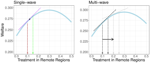
Figure 2: Example of experimental design, fixing the overall fraction of treated population to be half, and choosing between two types of individuals to treat (those in remote and non-remote regions). The left panel is a single-wave experiment with two clusters. In the first cluster, we assign the policy colored in green, and the second cluster colored in brown. The right panel is a two-wave experiment. We use a pair of clusters to estimate the marginal effect and update the policy for a different pair.

2.5 Main assumptions and applicability of the method

The proposed approach leverages two main assumptions: (i) the distribution of the network is the same across clusters; (ii) treatments do not generate heterogeneous effects in expectation across clusters. Here, (i) guarantees that, in expectation, the distribution of connections is comparable across different clusters. Condition (ii) guarantees that we can estimate marginal effects even with only two clusters. In the presence of unobserved heterogeneity, we would not be able to learn marginal effects when the number of clusters is small (finite).

The potential outcome model is consistent with models used in many applications, such as spillovers for agronomy advice (Duflo et al., 2023), and others (Cai et al., 2015; Miguel and Kremer, 2004; Crépon et al., 2013). All of these papers consider specifications with homogeneous effects across clusters. Researchers may test for homogeneity by comparing the average baseline covariates across different tehsils. We provide an empirical example in Table 2, where we show substantial homogeneity in our empirical application. In the presence of heterogeneity, however, we recommend appropriately re-weighting observations, formally discussed in Appendix A.4.

Finally, one additional assumption is no carry-over (dynamics) in treatment effects, common in adaptive experiments and Difference-in-Differences settings (e.g. Kasy and Sautmann, 2019; D’Haultfœuille et al., 2023), and common in economic applications (e.g. Duflo et al., 2023; Cai et al., 2015). In practice, carryovers do not occur if either each period $t$ is sufficiently far in time from the previous period or if the intervention only has short-term effects on the target outcome used in the experiment. We encourage researchers to appropriately choose the time window of each sequential update and the target outcome to guarantee that no dynamics occur. For example, in our application in Section 6, the treatment (providing weather forecast for the upcoming few days) affects short-term (one day ahead) predictions of weather (our target outcome) but not weather forecasts during the subsequent experimental wave (see Appendix C), hence satisfying the no dynamic effects assumption. We refer to Athey and Imbens (2018) for a discussion on the no carryovers assumption and Appendix A.2 for an extension of experiments with dynamic treatment effects.

Remark 5 (Super-population perspective).

This paper adopts a super-population perspective instead of a finite population perspective. This is useful due to unobserved connections and a finite number of clusters. In particular, a random network model allows us to control within-cluster dependence, and the focus on the out-of-sample regret on new clusters naturally requires restrictions on the potential outcomes’ (repeated) sampling. ∎

3 Single-wave experiment

In this section, we turn to the design and analysis of a single-wave experiment.

Definition 3.1 (Testable implication).

Let $\beta^{*}\in\mathcal{B}$ be an interior point. If $W(\beta)=W(\beta^{*})$, then

$$H_{0}:M^{(j)}(\beta)=0,\quad\forall j\in\{1,\cdots,p_{1}\},p_{1}\leq p.$$ (8)

The above implication is at the core of the proposed approach. We can test whether $p_{1}$ arbitrary entries of the marginal effect are equal to zero. Rejection implies a lack of global optimality. For expositional convenience, we consider $p_{1}=1$ only (test the first entry being zero). In Appendix A.5, we show how the proposed method generalizes to $p_{1}>1$. We may also test $M^{(j)}(\beta)\leq 0$; for example, for $\pi(x,\beta)=\beta_{x}$ (with $\mathcal{X}$ discrete), the one-sided test is informative for whether treatment probabilities for individuals with $x=j$ should be increased (without assuming that $\beta^{*}$ is in the interior). Finally, define the vector

$$\underline{e}_{j}=\begin{bmatrix}0,\cdots,0,1,0,\cdots,0\end{bmatrix},\text{ where }\underline{e}_{j}\in\{0,1\}^{p},\text{ and }\underline{e}_{j}^{(j)}=1.$$ (9)

Algorithm 2 presents the design. The algorithm pairs clusters. Within each pair, it estimates the first entry of the marginal effect using local perturbations. It then constructs a scale-invariant test statistics. Without loss of generality, we index clusters such that each pair contains two consecutive clusters $\{k,k+1\}$ with $k$ being an odd number.

Remark 6 (Pairing clusters).

For the sake of brevity, throughout the main text, we allow for arbitrary pairs in the design of Algorithm 2, by leveraging Assumption 2.2. In practice, pairing clusters may occur based on observed heterogeneity: similar clusters such as rural and urban areas should be paired together. We provide a formalization in Appendix A.4. ∎

Algorithm 2 One-wave experiment for inference with $p_{1}=1$

1:Value $\beta\in\mathbb{R}^{p}$ (exogenous), $K$ clusters, constant $\bar{C}$, size $\alpha$;

2:Organize clusters into $G=K/2$ pairs with consecutive indexes $\{k,k+1\}$;

3:For each pair $g=\{k,k+1\}$, $k$ is odd, run Algorithm 1, with at $t=1$,

$$D_{i,1}^{(k)}|\beta,X_{i}^{(k)}=x\sim\begin{cases}&\mathrm{Bern}(\pi(x,\beta+\eta_{n}\underline{e}_{1}))\text{ if }h=k\\ &\mathrm{Bern}(\pi(x,\beta-\eta_{n}\underline{e}_{1}))\text{ if }h=k+1\end{cases},\quad\bar{C}n^{-1/2}<\eta_{n}<\bar{C}n^{-1/4},$$

and estimate the marginal effect as in Equation (6).

4:Construct the t-statistic

$$\mathcal{T}_{n}=\frac{\sqrt{G}\bar{M}_{n}(\beta)}{\sqrt{(G-1)^{-1}\sum_{g}(\widehat{M}_{g}(\beta)-\bar{M}_{n}(\beta))^{2}}},\quad\bar{M}_{n}(\beta)=\frac{1}{G}\sum_{g}\widehat{M}_{g}(\beta);$$ (10)

here, $\widehat{M}_{g}$ is the marginal effect estimated in pair $g$.

5:Construct tests $1\Big{\{}|\mathcal{T}_{n}|>\mathrm{cv}_{G}(\alpha)\Big{\}}$ with size $\alpha$, with critical values as in Corollaries 1, 2.

3.1 Estimation of marginal and treatment effects

Algorithm 2 permits identifying the marginal effect, the direct effect, and the spillover effect.

Equation (6) provides the marginal effect estimator $\widehat{M}_{g}(\beta)$ for each pair of clusters $g$. Researchers may report $\bar{M}_{n}(\beta)$ (Equation 10) in their results – the average across clusters’ pairs. We show below that both $\bar{M}_{n}(\beta)$ and $\widehat{M}_{g}(\beta)$ provide a consistent estimate of $M^{(1)}(\beta)$. Our discussion directly extends to estimating each entry of $M(\beta)$ as shown in Appendix A.5.

The experiment also allows us to estimate the direct effect of the treatment and the (marginal) spillover effect separately, respectively under Assumption 3.1 below

$$\Delta(\beta)=\int\left[m(1,x,\beta)-m(0,x,\beta)\right]dF_{X}(x),\quad S_{1}(d,\beta)=\int\frac{\partial m(d,x,\beta)}{\partial\beta^{(1)}}dF_{X}(x).$$

The direct effect is the treatment effect, keeping fixed the neighbors’ treatment probability. $S_{1}(\cdot)$, the spillover effect, is the marginal effect of a small change in the first entry of $\beta$, keeping fixed individual treatment status. This setting also extends to estimating $S_{j}(\cdot)$ for arbitrary entries of $\beta$ as in Appendix A.5. For a given pair of clusters $(k,k+1)$, we estimate

$$\widehat{\Delta}_{k}(\beta) =\frac{1}{2n}\sum_{h\in\{k,k+1\}}\sum_{i=1}^{n}\left[\frac{D_{i,1}^{(h)}Y_{i,1}^{(h)}}{\pi(X_{i}^{(h)},\beta+\eta_{n}v_{h}\underline{e}_{1})}-\frac{(1-D_{i,1}^{(h)})Y_{i,1}^{(h)}}{1-\pi(X_{i}^{(h)},\beta+\eta_{n}v_{h}\underline{e}_{1})}\right],\quad v_{h}=\begin{cases}1\text{ if }h=k\\ -1\text{ if }h=k+1.\end{cases}$$ (11)

The estimator pools observations between the two clusters and takes a difference between treated and control units within each cluster, divided by the probability of treatments. This approach is similar to classical Horvitz-Thompson estimators (Horvitz and Thompson, 1952). We average direct effects across clusters’ pairs to obtain a single measure $\bar{\Delta}_{n}=\frac{1}{G}\sum_{g}\widehat{\Delta}_{g}(\beta)$. The indirect effect is estimated as follows:

$$\widehat{S}_{(k,k+1)}(0,\beta)=\frac{1}{2n}\sum_{h\in\{k,k+1\}}\frac{v_{h}}{\eta_{n}}\sum_{i=1}^{n}\left[\frac{Y_{i,1}^{(h)}(1-D_{i,1}^{(h)})}{1-\pi(X_{i}^{(h)},\beta+v_{h}\eta_{n}\underline{e}_{1})}-\bar{Y}_{0}^{(h)}\right].$$

The estimator takes a weighted difference between the two clusters’ control units. Researchers may report the between-pairs average $\bar{S}_{n}(0,\beta)=\frac{1}{G}\sum_{g}\widehat{S}_{g}(0,\beta)$ (and similarly $\hat{S}(1,\beta)$ for treated units), which captures spillovers on the control units.

Researchers may also be interested in estimating welfare effects at a given $\beta$, pooling information across clusters (here, $\bar{m}_{n}(0,\beta)$ estimates the average effect on the control units)

$$\bar{W}_{n}(\beta)=\frac{1}{K}\sum_{k=1}^{K}\Big{[}\bar{Y}_{1}^{(k)}-\bar{Y}_{0}^{(k)}\Big{]},\quad\bar{m}_{n}(0,\beta)=\frac{1}{nK}\sum_{k=1}^{K}\sum_{i=1}^{n}\left[\frac{Y_{i,1}^{(k)}(1-D_{i,1}^{(k)})}{1-\pi(X_{i}^{(k)},\beta+v_{h}\eta_{n}\underline{e}_{1})}-\bar{Y}_{0}^{(k)}\right].$$

3.2 Consistency and inference on the marginal effects

Next, we study theoretical guarantees.

Assumption 3.1 (Regularity 1).

Suppose that for all $x\in\mathcal{X},d\in\{0,1\}$, $\pi(x,\beta)$, and $m(d,x,\beta)$ are uniformly bounded and twice differentiable with bounded derivatives.

Assumption 3.1 imposes smoothness and boundedness restrictions. These restrictions hold for a large set of linear and non-linear functions, assuming that $\mathcal{X}$ is compact. Boundedness is often imposed in the literature (e.g., Kitagawa and Tetenov, 2018).

Theorem 3.1 (Marginal effects).

Suppose that $\varepsilon_{i,t}^{(k)}$ is sub-Gaussian. Let Assumptions 2.1, 2.2, 3.1 hold. Let $\mathrm{Var}(\sqrt{n}\hat{M}_{(k,k+1)}(\beta))\leq\tilde{C}_{k,k+1}\rho_{n}$, for arbitrary $\rho_{n}$ and constant $\tilde{C}_{k,k+1}$. Then, with probability at least $1-\delta$, for any $\delta\in(0,1)$, for a finite constant $c_{0}<\infty$ independent of $(n,N,\gamma_{N},K,\beta)$,

$$\Big{|}\hat{M}_{(k,k+1)}(\beta)-M^{(1)}(\beta)\Big{|}\leq c_{0}\left(\eta_{n}+\min\Big{\{}\sqrt{\frac{\gamma_{N}\log(\gamma_{N}/\delta)}{n\eta_{n}^{2}}},\sqrt{\frac{\tilde{C}_{k,k+1}\rho_{n}}{n\eta_{n}^{2}\delta}}\Big{\}}\right),$$

where $\hat{M}_{(k,k+1)}$ is estimated as in Algorithm 2.

For $\gamma_{N}\log(\gamma_{N})/N^{1/3}=o(1),\eta_{n}=n^{-1/3},\hat{M}_{(k,k+1)}(\beta)\rightarrow_{p}M^{(1)}(\beta),\bar{M}_{n}\rightarrow_{p}M^{(1)}(\beta)$.

The proof is in Appendix B.2.1. Theorem 3.1 shows one can consistently estimate the marginal effects with two large clusters. Consistency depends on the degree of dependence among unobservables $\varepsilon_{i,t}^{(k)}$ (which also depends on neighbors’ treatments). The convergence rate depends on the minimum between the maximum degree of the network, which is proportional to $\gamma_{N}^{1/2}$, and the covariances among unobservables, captured by $\rho_{n}$. If either the network has a degree that grows at a slower rate than $N$ (recall that $n/N=O(1)$) or a degree equal to $N$ but vanishing covariances, one can consistently estimate the marginal effects. The theorem also illustrates the trade-off in the choice of the deviation parameter $\eta_{n}$: a larger parameter $\eta_{n}$ decreases the variance, but it increases the bias. The reader may refer to Appendix F.3 for a rule of thumb for $\eta_{n}$.

Assumption 3.2 (Regularity 2).

Assume that for treatments as assigned in Algorithm 2, for all $k\in\{1,\cdots,K\}$, $\varepsilon_{i,t}^{(k)}$ has a bounded fourth moment, and for some $\bar{C}_{k}>0$, $\rho_{n}\geq 1$,

$$\mathrm{Var}\left(\sqrt{n}\Big{[}\bar{Y}_{1}^{(k)}-\bar{Y}_{0}^{(k)}\Big{]}\right)=\bar{C}_{k}\rho_{n}.$$ (12)

Assumption 3.2 imposes standard moment bounds and a lower bound on the variance of the estimator. In particular, Assumption 3.2 states that the variance does not converge to zero at a rate faster than $1/n$. To gain further intuition, note that

$$\bar{C}_{k}\rho_{n}=\frac{1}{n}\sum_{i=1}^{n}\mathrm{Var}\left(\varepsilon_{i,1}^{(k)}-\varepsilon_{i,0}^{(k)}\right)+\frac{1}{n}\sum_{i,j,j\neq i}\mathrm{Cov}\left(\varepsilon_{i,1}^{(k)}-\varepsilon_{i,0}^{(k)},\varepsilon_{j,1}^{(k)}-\varepsilon_{j,0}^{(k)}\right).$$ (13)

For bounded second moments, $\rho_{n}\leq\gamma_{N}+1$ from Lemma B.4, because each individual correlates with at most $\gamma_{N}$ many others. Assumption 3.2 is stating that $\rho_{n}\geq 1$, i.e., $\rho_{n}$ does not converge to zero. This requires that the negative covariance components (if any) do not outweigh the variances in Equation (13). This holds with no or positive outcomes correlations and guarantees that the variance is not degenerate at zero.

Theorem 3.2.

Let Assumptions 2.1, 2.2, 3.1, 3.2 hold. Let $n^{1/4}\eta_{n}=o(1),\gamma_{N}/N^{1/4}=o(1)$, $K<\infty$. Then, for each pair $(k,k+1)$, for $\widehat{M}_{(k,k+1)}$ estimated as in Algorithm 2,

$$\mathrm{Var}\Big{(}\widehat{M}_{(k,k+1)}\Big{)}^{-1/2}\Big{(}\widehat{M}_{(k,k+1)}-M^{(1)}(\beta)\Big{)}\rightarrow_{d}\mathcal{N}(0,1).$$

The proof is in Appendix B.2.2. Theorem 3.2 guarantees asymptotic normality. The theorem assumes that the maximum degree $\gamma_{N}^{1/2}$ grows at a slower rate than the sample size of order $N^{1/8}$ (and hence $n^{1/8}$ because $n$ is proportional to $N$). This condition is stronger than what is required for consistency only. Given Theorem 3.2, we conduct inference with scale-invariant test statistics without necessitating estimation of the (unknown) variance.

Corollary 1.

Let the conditions in Theorem 3.2 hold. For $4\leq K<\infty$, $\alpha\leq 0.08$,

$$\lim_{n\rightarrow\infty}P\Big{(}|\mathcal{T}_{n}|\leq\mathrm{cv}_{K/2}(\alpha)\Big{|}H_{0}\Big{)}\geq 1-\alpha,$$ (14)

where $\mathrm{cv}_{K/2}(h)$ is the size-$h$ critical value of a t-test with $K/2-1$ degrees of freedom.

The proof is in Appendix B.8. The theorem guarantees asymptotically valid inference on $H_{0}$ as $n\rightarrow\infty$ and $K$ is finite. With $p_{1}=1$, the proof is a direct consequence of Theorem 3.2, combined with properties of pivotal statistics in Ibragimov and Müller (2010). In Appendix A.5, we provide expressions for the test statistics and derivations for $p_{1}>1$.

An immediate corollary of Theorem 3.2 is also that randomization tests in Canay et al. (2017) are valid here for inference on the marginal effects (and similar results extend for inference on the direct and marginal spillover effects below). As argued in Canay et al. (2017), the benefits of randomization inference over Ibragimov and Müller (2010)’s method are its power and wide applicability since it is valid for all choices of $\alpha$.

Corollary 2 (Permutation tests).

Let the conditions in Theorem 3.2 hold. For any $\alpha\in(0,1)$, $\lim_{n\rightarrow\infty}P\Big{(}|\mathcal{T}_{n}|\leq\mathrm{cv}_{K/2}^{P}(\alpha)\Big{|}H_{0}\Big{)}=1-\alpha$, where $\mathrm{cv}_{K/2}^{P}(\alpha)$ is a $(1-\alpha)^{th}$ quantile of t-statistics computed from all permutations over the pairs’ sign as described in Appendix A.8.

To our knowledge, this set of results is the first for inference on welfare-maximizing policies with unknown interference.

3.3 Properties of direct, marginal spillover and welfare effects

We conclude this section with a study on the estimated direct, spillover, and welfare effects.

Theorem 3.3 (Asymptotically neglegible bias of treatment effects).

Let Assumptions 2.1, 2.2, 3.1 hold, and $\eta_{n}=o(n^{-1/4})$. Then, $\mathbb{E}\left[\bar{\Delta}_{n}(\beta)\right]=\Delta(\beta)+o(n^{-1/2})$, where the second term does not depend on $K$. Similarly, $\mathbb{E}\left[\bar{W}_{n}(\beta)\right]=W(\beta)+o(n^{-1/2}),\mathbb{E}\left[\bar{m}_{n}(0,\beta)\right]=m(0,\beta)+o(n^{-1/2})$, where the second term does not depend on $K$.

The proof is in Appendix B.2.3. The bias of the estimated direct effect is asymptotically negligible at a rate faster than the parametric rate $n^{-1/2}$ when pooling observations from different clusters. The main insight here is that, with pairing and perturbations of opposite signs, the first-order bias cancels out. Here, $\eta_{n}=o(n^{-1/4})$ is consistent with requirements in previous theorems. Given that the bias is asymptotically negligible, we can use existing results for inference. For completeness, we show consistency below.

Corollary 3.

Suppose $\varepsilon_{i,t}^{(k)}$ is sub-Gaussian. Let Assumptions 2.1, 2.2, 3.1 hold, and $\pi(x,\beta)\in(\kappa,1-\kappa),\kappa\in(0,1)$ for all $x\in\mathcal{X}$. Let $\eta_{n}=o(n^{-1/4})$. Then, with probability at least $1-3\delta$, for any $\delta\in(0,1)$, $\max\left\{\Big{|}\bar{\Delta}_{n}-\Delta(\beta)\Big{|},\Big{|}\bar{W}_{n}(\beta)-W(\beta)\Big{|},\Big{|}\bar{m}_{n}(0,\beta)-m(0,\beta)\Big{|}\right\}\leq c_{0}\left(\sqrt{\frac{\gamma_{N}\log(\gamma_{N}/\delta)}{Kn}}\right)+o(n^{-1/2}),$ for a finite constant $c_{0}<\infty$ independent of $(N,n,\gamma_{N},K,\beta)$.

The proof is in Appendix B.8. The corollary requires strict overlap (standard in the literature on causal inference) and shows that consistency for $K<\infty$, $n\rightarrow\infty$ can be attained. The following result is on the bias of the marginal spillover effects estimators (inference follows similarly to the marginal effect).

Theorem 3.4 (Marginal spillover effects).

Let Assumptions 2.1, 2.2, 3.1 hold. Then, for all pairs $(k,k+1)$, $\mathbb{E}\Big{[}\widehat{S}_{(k,k+1)}(0,\beta)\Big{]}=S_{1}(0,\beta)+\mathcal{O}(\eta_{n}).$

Remark 7 (Dependent clusters).

In some applications, clusters may only be approximately independent. In this case, inference is possible if between-clusters correlations are asymptotically negligible at an appropriate fast rate. In the presence of dependent clusters, we would need restrictions on the number of connections between clusters sufficiently smaller than $N$ and the maximum degree $\gamma_{N}$ growing at an appropriate slow rate.∎

4 Multi-wave experiment and welfare maximization

In this section, we design the adaptive experiment and derive its theoretical properties.

For illustrative purposes, we provide the algorithm for the one-dimensional case $p=1$, in Algorithm 3, that is, when $\beta\in\mathcal{B}=[\mathcal{B}_{1},\mathcal{B}_{2}]$ is a scalar. In Remark 8 and formally in Appendix E, we provide the complete algorithm for the $p$-dimensional case. Theoretical results are for the general $p$-dimensional case ($p$ is finite). Let $\hat{M}_{k,k+1}$ as in Equation (16).

Algorithm 3 Multiple-wave experiment with $\beta$ scalar

1:Starting value $\beta_{0}$, $K$ clusters, $T+1$ periods, constant $\bar{C}$.

2:Create pairs of clusters $\{k,k+1\},k\in\{1,3,\cdots,K-1\}$;

3:$t=0$ (initialization):

4:a: Assign treatments as $D_{i,0}^{(h)}|X_{i}^{(h)}=x\sim\mathrm{Bern}(\pi(x,\beta_{0}))\text{ for all }h\in\{1,\cdots,K\}.$

5:b: For $n$ units in each cluster observe $Y_{i,0}^{(h)},h\in\{1,\cdots,K\}$; initalize $\widehat{M}_{k,t}=0$, $\check{\beta}_{k}^{0}=\beta_{0}$.

6:while $1\leq t\leq T$ do

7:a: Define

$$\check{\beta}_{h}^{t}=\begin{cases}&P_{\mathcal{B}_{1},\mathcal{B}_{2}-\eta_{n}}\Big{[}\check{\beta}_{h}^{t-1}+\alpha_{h+2,t}\widehat{M}_{h+2,t-1}\Big{]},\quad h\in\{1,\cdots,K-2\},\\ &P_{\mathcal{B}_{1},\mathcal{B}_{2}-\eta_{n}}\Big{[}\check{\beta}_{h}^{t-1}+\alpha_{1,t}\widehat{M}_{1,t-1}\Big{]},\quad\quad\quad h\in\{K-1,K\};\end{cases}$$

where $\alpha_{k,t}$ is the learning rate $P_{a,b}(x)=\mathrm{arg}\min_{x^{\prime}\in[a,b]^{p}}||x-x^{\prime}||^{2}$.

8:b: Assign treatments as (for $\bar{C}n^{-1/2}<\eta_{n}<\bar{C}n^{-1/4}$)

$$D_{i,t}^{(h)}|X_{i}^{(h)}=x\sim\mathrm{Bern}(\pi(x,\beta_{h,t})),\quad\beta_{h,t}=\begin{cases}&\check{\beta}_{h}^{t}+\eta_{n}\text{ if }h\text{ is odd}\\ &\check{\beta}_{h}^{t}-\eta_{n}\text{ if }h\text{ is even}\end{cases}$$ (15)

9:c: For $n$ units in each cluster $h\in\{1,\cdots,K\}$ observe $Y_{i,t}^{(h)}$;

10:d: For each pair $\{k,k+1\}$, estimate

$$\hat{M}_{k,t}=\hat{M}_{k+1,t}=\frac{1}{2\eta_{n}}\Big{[}\bar{Y}_{t}^{(k)}-\bar{Y}_{0}^{(k)}\Big{]}-\frac{1}{2\eta_{n}}\Big{[}\bar{Y}_{t}^{(k+1)}-\bar{Y}_{0}^{(k+1)}\Big{]}.$$ (16)

11:end while

12:     Return $\hat{\beta}^{*}=\frac{1}{K}\sum_{k=1}^{K}\check{\beta}_{k}^{T}$

The algorithm pairs clusters and initializes clusters at the same starting value $\beta_{0}$, $\check{\beta}_{1}^{1}=\cdots=\check{\beta}_{K}^{1}=\beta_{0}$. At $t=0$, it randomizes treatments independently as

$$t=0:\quad D_{i,t}^{(k)}|X_{i}^{(k)}=x\sim\pi(x;\beta_{0}),\quad\text{ for all }(i,k).$$

Here, $\beta_{0}$ is chosen exogenously, e.g., it is the current policy in place. Over each iteration $t$, we assign treatments based on $\beta_{k,t}$ for cluster $k$ at time $t$, which equals the parameter $\check{\beta}_{k}^{t}$ obtained from a previous iteration plus a positive (negative) perturbation $\eta_{n}$ in the first (second) cluster in a pair. The local perturbation follows similarly to what is discussed in the previous section. Also, by construction, $\check{\beta}_{k}^{t}$ is the same for a given pair $(k,k+1)$, where $k$ is odd. We choose $\check{\beta}_{k}^{t+1}$ via sequential cross-fitting: we wrap clusters in a circle and update the parameter in a pair of clusters $(k,k+1)$ using information from the subsequent pair (see Figure 4). The algorithm runs over $T$ periods and returns $\hat{\beta}^{*}=\frac{1}{K}\sum_{k=1}^{K}\check{\beta}_{k}^{T+1}.$ Choosing the average is motivated by the theoretical properties of gradient descent methods, although other statistics are also possible.

In the proposed experiment, we update the policy in each clusters pair with information from a subsequent pair to guarantee unconfoundedness.

Lemma 4.1 (Unconfoundedness).

Let $T/p+1\leq K/2$. Consider the experimental design in Algorithm E.2 for generic $p$-dimensions (and Algorithm 3 for $p=1$). Then, for any $k$,

$$\Big{(}\beta_{k,1},\cdots,\beta_{k,T}\Big{)}\perp\Big{\{}Y_{i,t}^{(k)}(\mathbf{d}),X_{i}^{(k)},\mathbf{d}\in\{0,1\}^{N}\Big{\}}_{i\in\{1,\cdots,N\},t\leq T}.$$

The proof is in Appendix B.1.4. Lemma 4.1 shows that the parameters used in the experiment are independent of potential outcomes and covariates in the same cluster. Namely, the sequential cross-fitting breaks the dependence due to repeated sampling, which would otherwise confound the experiment. The main distinction from most of the previous literature on adaptive experiments (e.g. Kasy and Sautmann, 2019; Wager and Xu, 2021; Hadad et al., 2019; Zhang et al., 2020) is that in all such references where repeated sampling does not occur, and batches are independent each period. Here, instead, clusters are dependent over each period, motivating our sequential estimation procedure. Sequential cross-fitting guarantees unconfoundedness by updating policies for a given cluster’s pair using information from the previous pair only. Its goal is to guarantee unbiased estimated marginal effects.

Remark 8 ($p$-dimensional case: Algorithm E.2).

The algorithm for the $p$-dimensional case follows similarly to the uni-dimensional case with a minor change: we consider $T/p$ many waves/iterations, each consisting of $p$ periods. Within each wave $w$, every period, we perturb a single coordinate of $\check{\beta}_{k}^{w}$, compute the marginal effect for that coordinate, and repeat over all coordinates $j\in\{1,\cdots p\}$ before making the next policy update to select $\check{\beta}_{k}^{w+1}$. ∎

Remark 9 (Learning rate).

We are now left to discuss how “large” the step size should be: if the marginal effect is positive, by how much should we increase the treatment probability? Assuming strong concavity of the objective function, the learning rate $\alpha_{k,t}$ should be of order $1/t$. A more robust choice (see Theorem A.8) is

$$\alpha_{k,t}=\begin{cases}&\frac{J}{T^{1/2-v/2}||\hat{M}_{k,t}||}\text{ if }||\hat{M}_{k,t}||_{2}^{2}>\frac{\kappa}{\check{T}^{1-v}}-\epsilon_{n},\\ &0\text{ otherwise}\end{cases},$$ (17)

for a positive $\epsilon_{n}$, $\epsilon_{n}\rightarrow 0$, and small constants $1\geq v,\kappa>0$. Here, the learning rate divides the estimated marginal effect by its norm (known as gradient norm rescaling, Hazan et al. 2015) and guarantees control of the out-of-sample regret under strict quasi-concavity. This choice is appealing because it guarantees comparable step sizes between different clusters. ∎

Remark 10 (Why sequential cross-fitting?).

Next, we illustrate the source of bias if the sequential cross-fitting was not employed. Every period, the researcher can only identify the expected outcome of $Y_{i,t}^{(k)}$ conditional on the parameter $\beta_{k,t}$, namely $\widetilde{W}(\beta_{k,t})=\mathbb{E}_{\beta_{k,t}}[Y_{i,t}^{(k)}|\beta_{k,t}].$ If $\beta_{k,t}$ were chosen exogenously, based on information from a different cluster, $\mathbb{E}_{\beta_{k,t}}[Y_{i,t}^{(k)}|\beta_{k,t}]=\mathbb{E}_{\beta_{k,t}}[Y_{i,t}^{(k)}]=W(\beta_{k,t})$, where $W(\beta_{k,t})$ defines the expected welfare once we deploy the policy $\beta_{k,t}$ on a new population. However, the equality conditional and unconditional on $\beta_{k,t}$ does not occur when $\beta_{k,t}$ is estimated using information on $Y_{i,t-1}^{(k)}$. Consider the example where the outcome depends on some auto-correlated unobservables $\nu_{i,t}$ and treatment assignments in Figure 3. The dependence structure of Figure 3 implies: $W(\beta_{k,t})=\mathbb{E}_{\beta_{k,t}}[Y_{i,t}^{(k)}]\neq\mathbb{E}_{\beta_{k,t}}[Y_{i,t}^{(k)}|\beta_{k,t}]=\widetilde{W}(\beta_{k,t}),$ if $\beta_{k,t}$ depends on covariates and unobservables previous outcomes (and so on unobservables $\nu_{i,t}^{(k)}$) in cluster $k$. Here, $W(\beta_{k,t})$ captures the estimand of interest. Instead, $\widetilde{W}(\beta_{k,t})$ denotes what we can identify. The proposed algorithm breaks such dependence and guarantees unconfounded experimentation. ∎

Figure 3: The left panel shows the dependence structure when a static policy is implemented on a new population (I omit $D_{i,t-1}^{(k)}$ for expositional convenience). The right panel shows the dependence structure of a sequential experiment that uses the same units for policy updates over subsequent periods in the presence of repeated sampling.

Figure 4: sequential cross-fitting method. Clusters (rectangles) are paired. Within each pair, researchers assign different treatment probabilities to clusters with different colors. Finally, the policy in each pair is updated using information from the consecutive pair. Note that because $K>2T$, the algorithm never “circles back” to the initial pair.

4.1 Theoretical guarantees

Next, we derive theoretical properties. Let $\check{T}=T/p$. We assume the following.

Assumption 4.1.

Let (A) $\varepsilon_{i,t}^{(k)}$ be sub-Gaussian; and (B) $K\geq 2(T/p+1)$.

Condition (A) states that unobservables have sub-Gaussian tails (attained by bounded random variables); (B) assumes that the number of clusters is at least twice the number of waves, which guarantees that Lemma 4.1 (unconfoundedness) holds.

In the following results, we impose the following restriction.

Assumption 4.2 (Strong concavity).

Assume $W(\beta)$ is $\sigma$-strongly concave, for some $\sigma>0$ (i.e., $W(\beta)$’s Hessian is strictly negative definite).

A simple example of strong concavity is Example 2.1, where neighbors’ effects induce decreasing marginal effects, and the treatment may present some costs. We provide an illustration of this example by calibrating to real-world data in Figure 2. Strong concavity also arises in linear models with negative externalities (e.g. Crépon et al., 2013), as shown in Example 2.2. Both Examples 2.1 and 2.2 hold for any network formation process. Assumption 4.2 fails when spillovers occur only after that “enough” individuals have received the treatment. To accommodate this setting, we relax Assumption 4.2 in Appendix A.6, allowing for a strictly quasi-concave objective that is best suited for these settings, as in our application in Section 6. Settings where Assumption 4.2 fails are those where also the network changes with the intervention, left to future research. In these cases, the proposed method returns a local optimum. Finally, when using multiple starting values of our adaptive algorithm, we only require concavity locally with respect to each starting value.

Theorem 4.2.

Let Assumptions 2.1, 2.2, 3.1, 4.1, 4.2 hold. Take a small $1/4>\xi>0$, $\alpha_{k,w}=J/w$ for a finite $J\geq 1/\sigma$. Let $n^{1/4-\xi}\geq C\sqrt{p\log(n)\gamma_{N}T^{Bp}\log(KT)}$, $\eta_{n}=1/n^{1/4+\xi}$, for finite constants $B,C>0$. Then, with probability at least $1-1/n$, for a constant $\bar{C}^{\prime}<\infty$, independent of $(p,n,N,K,T)$, $||\beta^{*}-\hat{\beta}^{*}||^{2}\leq\frac{p\bar{C}^{\prime}}{\check{T}}.$

The proof is in Appendix B.2.5. Theorem 4.2 provides a bound on the distance between the estimated policy and the optimal one. The bound depends only on $T$ (and not $n$) because $n$ is assumed to be sufficiently larger than $T$.

Corollary 4.

Let the conditions in Theorem 4.2 hold. Let $K=2(T/p+1)$. Then with probability at least $1-1/n$, $W(\beta^{*})-W(\hat{\beta}^{*})\leq\frac{pC^{\prime}}{K},$ for a constant $C^{\prime}<\infty$ independent of $(p,n,N,K,T)$.

The proof is in Appendix B.8. The corollary formalizes the out-of-sample regret bound for $K=2(T/p+1)$. Also, the rate in $K$ does not depend on $p$, as $n\rightarrow\infty$. This is different from grid-search procedures, where the rate in $K$ would be exponentially slower in $p$. Researchers may wonder whether the procedure is “harmless” also on the in-sample units.

Theorem 4.3 (In-sample regret).

Let the conditions in Theorem 4.2 hold. Then, with probability at least $1-1/n$, for a constant $c<\infty$ independent of $(p,n,N,K,T)$,

$$\max_{k\in\{1,\cdots,K\}}\frac{1}{\check{T}}\sum_{w=1}^{\check{T}}\Big{[}W(\beta^{*})-W(\check{\beta}_{k}^{w})\Big{]}\leq c\frac{p\log(\check{T})}{\check{T}}.$$

The proof is in Appendix B.2.6. Theorem 4.3 guarantees that the cumulative welfare in each cluster $k$, incurred by deploying the current policy $\check{\beta}_{k}^{w}$ at wave $w$ (recall that in the general $p$-dimensional case we have $\check{T}$ many waves), converges to the largest achievable welfare at a rate $\log(T)/T$, also for those units participating in the experiment. This result guarantees that the proposed design controls the regret on the experiment participants. We conclude by deriving a faster (exponential) convergence rate of the out-of-sample regret (but not in-sample regret) with a different choice of the learning rate.

Theorem 4.4 (Out-of-sample regret with larger sample size).

Let Assumptions 2.1, 2.2, 3.1, 4.1, 4.2 hold, with $W(\beta)$ being $\tau$-smooth, and $K=2T+2$. Take a small $1/4>\xi>0$, $\alpha_{k,w}=1/\tau$. Let $n^{1/4-\xi}\geq C\sqrt{p\log(n)\gamma_{N}e^{TBp}\log(KT)}$, $\eta_{n}=1/n^{1/4+\xi}$, for finite constants $B,C>0$. Then, with probability at least $1-1/n$, for constants $0<c_{0},c_{0}^{\prime}<\infty$, independent of $(n,N,K,T)$,

$$W(\beta^{*})-W(\hat{\beta}^{*})\leq c_{0}\exp(-c_{0}^{\prime}K).$$

The proof is in Appendix B.2.7. The main restriction is that the sample size grows exponentially in the number of iterations (instead of polynomially). The theorem leverages properties of the gradient descent under strong concavity and smoothness (Bubeck et al., 2012). Fast rates for the out-of-sample regret are achieved under an appropriate choice of the learning rate that leverages the smoothness of the objective function. The choice of a learning rate invariant in the iteration $t$ requires a sample size exponential in $T$. This differs from the choice of a learning rate as $1/t$ in Theorem 4.2, where the adaptive learning rate enables controlling the cumulative error polynomially in $n$. To our knowledge, these regret guarantees are the first under unknown (and partial) interference.

We now contrast the above results with past literature. In the online optimization literature, the rate $1/T$ is common for convex optimization, assuming independent units (see Duchi et al., 2018, for out-of-sample regret rates). Here, because of interference, we leverage between-clusters perturbations. Also, we do not have direct access to the gradient, and related optimization procedures are those in the literature on zero-th order optimization (Kiefer and Wolfowitz, 1952). Flaxman et al. (2004); Agarwal et al. (2010) in particular are related to our approach, where regret can converge at rate $O(1/T)$ in expectation only, whereas high-probability bounds are $1/\sqrt{T}$ (see Theorem 6 in Agarwal et al., 2010, and the discussion below). Here, we exploit within-cluster concentration and between clusters’ variation to control for large deviations of the estimated gradients and obtain faster rates for high-probability bounds. This approach also allows us to extend out-of-sample guarantees beyond global strong concavity (assumed in the above references) in Appendix A.6. In our derivations, the perturbation parameter depends on the sample size, differently from the references above, and the idea of sequential estimation is novel due to repeated sampling. Wager and Xu (2021) derive $1/T$ regret guarantees in the different settings of market pricing, as $n\rightarrow\infty$, with independent units and samples each wave. Our results do not impose independence or modeling assumptions other than partial interference. Viviano (2019) considers a single network, with observed neighbors of experiment participants, instead of a sequential experiment. He imposes geometric (VC) restrictions on the policy and solves a mixed-integer linear program. Here, we introduce an adaptive experiment and we do not require network information, using network concentration not studied in previous works.

These differences require a different set of techniques for derivations. The proof of the theorem (i) uses concentration arguments for locally dependent graphs (Janson, 2004); (ii) uses the within-cluster and between-clusters variation for consistent estimation of the marginal effect, together with the cluster pairing; (iii) it uses a recursive argument to bound the cumulative error obtained through the estimation and sequential cross-fitting.

5 The value of network data

Next, under more restrictive conditions, we ask how $\beta^{*}$ compares with the policy that assigns treatments without restrictions on the policy function. We omit the super-script $k$ because the argument below applies to any cluster. Consider

$$W_{N}^{*}-W(\beta^{*}),\quad W_{N}^{*}=\sup_{\mathcal{P}_{N}(\cdot)\in\mathcal{F}}\frac{1}{N}\sum_{i=1}^{N}\mathbb{E}\Big{[}\mathbb{E}_{D\sim\mathcal{P}_{N}(A,X)}[Y_{i,t}|A,X]\Big{]}$$ (18)

with $\mathcal{F}$ as the set of all conditional distribution of the vector $D\in\{0,1\}^{N}$, given network $A$ and the covariates of all observations $X$. Equation (18) denotes the difference between the expected outcomes, evaluated at the global optimum over all possible assignments (once both $A,X$ are observed), and the welfare evaluated at $\beta^{*}$ (without observing the network).

Assumption 5.1 (Discrete parameter space, assignment, and minimum degree).

Assume that $X_{i}\in\mathcal{X},\mathcal{X}=\{1,\cdots,|\mathcal{X}|\},|\mathcal{X}|<\infty,P(X=x)>\bar{\kappa}>0$ for all $x\in\mathcal{X}$. Let $\pi(x,\beta)=\beta_{x}$, and $\mathcal{B}=[0,1]^{|\mathcal{X}|}$. Also, let $\inf_{x,x^{\prime},u^{\prime}}\int l(x,u,x^{\prime},u^{\prime})dF_{U|X=x}(u)\geq\underline{\kappa}$, for some $\underline{\kappa},\bar{\kappa}\in(0,1]$.

Assumption 5.1 states that researchers assign treatments based on finitely many observable types as in Manski (2004), Graham et al. (2010). Each type $x\in\mathcal{X}$ is assigned a different probability $\beta_{x}$, which can take any value between zero and one. Assumption 5.1 also states that conditional on individual’s type $(X_{i},U_{i})$, any other unobserved type $U_{j}$ can form a connection with individual $i$ with some positive probability, provided that $i$ and $j$ are connected under the latent space representation (recall Equation 1). This condition is consistent with Assumption 2.1, because the assumption states that the expected minimum degree is bounded from below by $\underline{\kappa}\gamma_{N}^{1/2}$, which is smaller than the maximum degree $\gamma_{N}^{1/2}$. The second restriction is on the potential outcomes. Let

$$Y_{i,t}(\mathbf{d}_{t}) =\Big{[}\Delta(X_{i})-v(X_{i})\Big{]}\mathbf{d}_{i,t}+\mathcal{S}_{i,t}(\mathbf{d}_{t})+\nu_{i,t},\quad\mathbb{E}[\nu_{i,t}|X,A]=0$$ (19)

$$\mathcal{S}_{i,t}(\mathbf{d}_{t}) =s\Big{(}\frac{\sum_{j=1}^{n}A_{i,j}\mathbf{d}_{j,t}1\{X_{j}=1\}}{\sum_{j=1}^{n}A_{i,j}1\{X_{j}=1\}},\cdots,\frac{\sum_{j=1}^{n}A_{i,j}\mathbf{d}_{j,t}1\{X_{j}=|\mathcal{X}|\}}{\sum_{j=1}^{n}A_{i,j}1\{X_{j}=|\mathcal{X}|\}}\Big{)},$$

where $0/0=0$. Here, $\Delta(\cdot)$ is the direct treatment effect, and $v(\cdot)$ is the cost of the treatment. The function $s(\cdot)$ captures the spillover effects. Spillovers depend on the fraction of treated neighbors, are heterogeneous in the neighbors’ types, with no interactions with direct effects.

Theorem 5.1.

Let Equation (19) hold, with $s(\cdot)$ twice differentiable with bounded derivatives. Suppose that Assumption 2.1, 2.2, 5.1 hold. Then, with $W_{N}^{*}$ as in Equation (18), $\lim_{N,\gamma_{N}\rightarrow\infty}\Big{\{}W_{N}^{*}-W(\beta^{*})\Big{\}}\leq\mathbb{E}\Big{[}|\Delta(X)-v(X)|\Big{]}.$

The proof is in Appendix B.2.8. Theorem 5.1 bounds the welfare difference by the expected direct effects minus costs. If direct effects are small compared with the treatment costs, such a difference is negligible (for any spillover effects). The bound is identified without network data under separability of direct and spillover effects. The theorem assumes that the maximum degree converges to infinity, but it may converge at a slower rate than $N$, consistent with our conditions in previous theorems. This result is novel in the context of the literature on targeting networked individuals and provides a formal characterization of the value of collecting network information. Theorem 5.1 does not state that spillovers are not relevant ($\beta^{*}$ depends on the spillovers). Instead, it states that one can compute best policies, without knowledge of the network in settings where direct effects are small.

One can estimate the bound by taking an absolute difference between the treated and control units for different individual types, and average across types. In Example 2.1, the bound equals $\phi_{1}$ (the direct treatment effect) minus the cost of implementing the treatment.

Corollary 5.

Let the conditions in Theorem 5.1 hold. Let $C_{e}$ be the cost of collecting network information per individual (with total cost for observing the network $A$ equal to $NC_{e}$). Then, $\lim_{N,\gamma_{N}\rightarrow\infty}W_{N}^{*}-W(\beta^{*})-C_{e}\leq 0$, if $C_{e}\geq\mathbb{E}\Big{[}|\Delta(X)-v(X)|\Big{]}$.

A second interesting case is when costs define the opportunity costs as below.

Assumption 5.2 (Costs are opportunity costs of an equal-impact intervention with no spillovers).

Assume $\Delta(x)=v(x)$ for all $x\in\mathcal{X}$.

Assumption 5.2 states that the cost of the treatment is the opportunity cost, had the treatment been assigned to the same individuals that are disconnected. For instance, researchers may assign treatments to individuals in the same or nearby villages or to individuals spread out over an entire state without creating spillovers. The cost of the treatment to assign treatments in the same villages is their opportunity cost, i.e., the direct effects.

Corollary 6.

Let the conditions in Theorem 4.2 and Theorem 5.1, and Assumption 5.2 hold. Then, $\lim_{N\rightarrow\infty,\gamma_{N}\rightarrow\infty}W_{N}^{*}-W(\beta^{*})\rightarrow 0$.

6 Field experiment

We study the properties of the proposed design in a field experiment that provided geo-localized weather forecasts to over 400,000 cotton farmers in Pakistan. The experiment was implemented through Precision Development (PxD), an NGO that provides farmers with phone-based agricultural advisory services. In partnership with a private forecast provider, Precision Development developed calibrated (geo-localized) weather forecast information localized at the tehsil level (tehsils are administrative units equivalent to US counties). The treatment consists of calling farmers to provide weather forecasts via robocalls, meant to improve farmers’ ability to take adaptive measures in their cotton plots. In a survey, $80\%$ of the respondents said they actively shared weather information with other farmers.

Farmers often lack access to geo-localized weather forecasts, and digital advice offers solutions to address this challenge (Fabregas et al., 2019). Before the experiment, PxD conducted a set of interviews with farmers. “While 71% of wheat farmers cited access to weather forecasting information, only 45% of cotton farmers surveyed reported access to weather information. When asked if weather information “helped in planning”, 88 and 86% of cotton and wheat respondents respectively responded in the affirmative.”(https://precisiondev.org/weather-forecasting-product-for-punjab-pakistan/). In addition, those farmers with access to weather forecasts only access forecasts produced at the district level, a higher administrative unit that typically includes 3-4 tehsils.

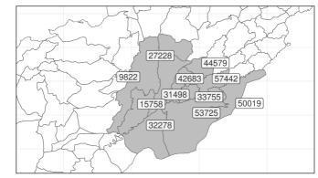
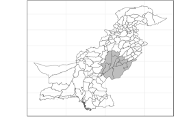
Figure 5: Pakistan’s map, organized in districts (each district contains multiple tehsils). Gray regions indicate areas selected for the experiment. Next to each district, we report the total sample size obtained from the tehsils in the experiment in the given district.

6.1 Experimental design and data sources

We deployed the design presented in Section 3 over two consecutive waves. The first wave started in April 2022, during which approximately half of the population was exposed to treatment, and the second wave started in August 2022, during which the NGO increased the total number of treated individuals due to exogenous operational constraints. Because marginal effects suggest increasing treatment probabilities from the first to the second wave (see Section 6.4), the second wave allows us to compute counterfactual improvement of an adaptive (two-wave) experiment that follows the marginal effects as in Section 4.

In total, 40 tehsils were exposed to experimental variation. Figure 5 illustrates the region in Pakistan exposed to experimental variation and the sample size within each district (not all tehsils in a district are in the experiment). Tehsils have sample sizes ranging from 5,000 to 20,000 farmers enrolled in the program. We consider a tehsil a cluster. The underlying assumption is that spillovers between different tehsils are negligible, here justified by the fact that tehsils denote large geographic areas, and forecasts are geo-localized at the tehsil level. In contrast to some prior work (e.g., Banerjee et al., 2013), our design allows for spillovers across villages in the same tehsil.

We design the first experimental wave (April - July) as follows. We randomly draw a group of twelve tehsils (“Medium Saturation”) to have an average treatment probability of $\beta=0.4$. We induce local perturbations ($\eta_{n}=0.05$) between different tehsils, with six tehsils assigned to treatment probabilities $0.35$ and the remaining six to $0.45$. We repeat a similar process with thirteen tehsils assigned to higher treatment probability $\beta=0.6$ (“Higher Saturation”). The “Medium Saturation” and “Higher Saturation” samples follow the same design of local perturbation as in Section 3, while we also consider a third group, “Lower Saturation”, with a different design, which assigns tehsil-specific perturbations to treatment probabilities, with $\beta=0.11$ on average, but without inducing perturbations as in the other groups. Each group of tehsils was stratified across districts. We use information from all clusters for our regression analysis and use the Medium and High Saturation groups to compute the marginal effects since these groups closely follow our design in Section 3.

We increased treatment probabilities for each tehsil during the second wave in August 2022. Therefore, medium saturation tehsils with treatment probability $\beta=0.4$ were exposed to treatment probability $\beta=0.6$, high saturation tehsils increased the average treatment probability from $\beta=0.6$ to $\beta=0.8$, and low saturation tehsils went from $\beta=0.11$ to $\beta=0.25$ (see Table 1). During the second wave, the Medium Saturation group was exposed to an overall treatment probability exactly equal to $60\%$, and the Higher Saturation group to $80\%$ treatment probability. The second wave experiment allows us to compute marginal effects around $\beta=0.7$ by comparing Medium and Higher Saturation clusters. Finally, due to exogenous operational constraints from PxD, five additional tehsils were assigned to a different treatment arm from the main treatment arm during the first wave, during which additional information was provided together with the weather forecasts. These five tehsils were then assigned to the main treatment arm with Higher Saturation over the second wave. We exclude survey information from these tehsils collected during the first but not the second wave (results are robust if we also exclude these tehsils during the second wave).

	Number of Farmers	Number of Tehsils	$\beta$ (April - July)	$\beta$ (Aug - Sept)
Medium Saturation	137 729	12	0.4 ($\pm 0.05$)	0.6
Higher Saturation	149 758	13	0.6 ($\pm 0.05$)	0.8
Lower Saturation	111 300	10	0.11	0.25

Table 1: Statistics of the experiment. $\beta$ indicates the average treatment probability across each group of tehsils. Within each group of the medium and higher saturation, we assigned half of the tehsils to $\beta+0.05$ and the other half to $\beta-0.05$ in the first wave. For lower saturation, we assigned different probabilities to each tehsil. Over the second wave, we induced perturbations to treatment probabilities for two farmer types, with overall constant treatment probability.

We use two main data sources: (i) data about baseline covariates and response rates available on a daily basis for all farmers enrolled in the program; (ii) repeated high-frequency (daily) cross-sectional survey data collected from June to October 2022, with, in total approximately $6000$ respondents, stratified across tehsils and individual treatment status. Survey data provides us with information about farmers’ expectations for next-day weather and farming behavior, such as the use of irrigation, pesticides, and others. We merge this information with real geo-localized (satellite) weather information and PxD forecasts.

6.2 Balance and treatment efficacy

As a first exercise, we document balance across different clusters in Table 2, where we report the sample means across observable baseline covariates: the overall number of individuals in the experiment in each cluster, whether individuals have only attended primary or no education, the percentage of female farmers, the size of landholding in acres, the number of male and female dependants, the farmer’s age, whether farmers are also wheat farmers, and whether they have the mobile app “Whatsapp”. We test for differences in covariates between clusters exposed to positive and negative perturbations within each group of interest (medium and high saturation). We also test for differences between the medium and high saturation group. We compute p-values via randomization inference as in Section 3. These tests are informative of whether such groups are comparable and are conducted with a large sample size ($n\approx 10,000$ on average in each tehsil). We observe very similar estimates across all covariates. The smallest p-value is $0.21$, while the median p-value is above $0.5$. These results provide evidence of similar characteristics across different comparison groups.

As a second exercise, in Table 3, we collect raw information on response rates of treated and control farmers, pooled across all tehsils. The treatment group received approximately three times more frequent calls than the control group by design – where the control group’s calls were about other activities of the NGO. Table 3 shows that the larger number of calls does not negatively affect response rates. Instead, treated individuals are more engaged and present higher (and statistically significant at the $1\%$ level) response rates per call. This result suggests that farmers in the program actively engaged with weather forecasts.

As a third exercise, we measure the accuracy of the forecasts provided by the NGO with respect to the real weather in Table 4. On average, the forecast correctly predicts whether it (or it does not) rains $80\%$ of the time. Forecast and real precipitation and temperature are strongly positively correlated, with p-values equal to zero after clustering at the tehsil level.

Saturation	Medium			High			Medium/High
First wave $\beta=$	$0.35$	$0.45$		$0.55$	$0.65$		$0.4\pm 0.05$	$0.6\pm 0.05$
# of Farmers	11817	11137		10031	12795		11477	11519
(p-value)	(0.875)			(0.718)			(0.982)
Education	0.539	0.515		0.564	0.595		0.527	0.583
(p-value)	(0.875)			(0.875)			(0.211)
Female	0.016	0.019		0.021	0.031		0.018	0.026
(p-value)	(0.500)			(0.250)			(0.223)
Acres	4.158	4.159		4.468	4.067		4.158	4.228
(p-value)	(0.875)			(0.562)			(0.901)
Male Dependants	2.491	2.795		2.606	2.669		2.639	2.644
(p-value)	(0.593)			(0.937)			(0.988)
Female Dependants	2.485	2.750		2.645	2.637		2.613	2.641
(p-value)	(0.718)			(1)			(0.942)
Age	50.9	51.5		50.9	50.9		51.2	50.9
(p-value)	(0.937)			(1)			(0.970)
Wheat	0.644	0.510		0.470	0.546		0.579	0.515
(p-value)	(0.562)			(0.343)			(0.617)
Whatsapp	0.257	0.295		0.263	0.273		0.276	0.269
(p-value)	(0.812)			(0.937)			(0.702)

Table 2: Clusters’ balance table. Each entry reports the average value of a given baseline characteristic for clusters exposed to different treatment probabilities. Each column collects results for two groups of clusters. P-values test the two-sided null hypothesis that the point estimates for the two groups are different and are computed via randomization inference.

	$n$	Calls/Person	Total Response/Person	Average Response
Treated	158 697	110	26	0.236
Controls	240 354	45	10	0.222
$p$-value Response				[0.000]

Table 3: Summary statistics of treated and control units for May - July (Wave 1), pooled across all tehsils in the experiment. $p$-value is obtained via randomization inference at the cluster level.

	Dependent variable:
	Real Precipitation	Real Temperature Max	Correct Rain Forecast
Forecast Precipitation	0.675∗∗∗
	(0.020)
Forecast Temperature Max		0.914∗∗∗
		(0.029)
Constant	1.585∗∗∗	0.274	0.786∗∗∗
	(0.069)	(1.112)	(0.005)
Note:	∗p$<$0.1; ∗∗p$<$0.05; ∗∗∗p$<$0.01

Table 4: Forecast vs real weather in 2022. Sample size equal to 22230. The first column uses precipitation as a continuous variable and the last column regresses the indicator of whether the forecast of whether it will rain correctly predicts whether it rains. In parenthesis standard errors clustered at the tehsil level.

6.3 Farmers’ beliefs and activities: linear regression

Our design can accommodate standard regression analysis. Before presenting the results on optimal policies, we present regression estimates to study how the intervention affects farmers’ beliefs about the weather and farming activities, focusing on linear models. We consider non-linear models in the following subsection.

To measure farmers beliefs, we use two survey questions asked during a survey collected throughout June to October 2022 during the experiment: (i) “What do you expect will be the maximum temperature in your area tomorrow?” and (ii) “Do you think it will rain in your area tomorrow?” We merge this information with forecast weather and actual weather the day after the survey interview with the specific farmer. We measure the absolute difference between the farmer’s predicted maximum temperature and the PxD forecast maximum temperature. We also measure the difference between the farmer’s prediction and the realized maximum temperature the day after the interview. Temperature variables define incorrect beliefs, i.e., negative treatment effects indicate when that farmer’s prediction is closer to the PxD forecast or actual temperature. We construct similar variables for predicted rains where we measure whether the farmers incorrectly predict no rain and instead, it rains, or vice versa. Table 4 shows that PxD forecast rain is a predictive but noisy proxy for real rain and similarly for temperature. Therefore, we expect that results about farmers’ beliefs relative to PxD forecasts follow similar patterns with respect to farmers’ beliefs about realized weather, but beliefs about PxD forecasts are less noisy.

For a preliminary analysis, we consider a regression specification of the outcome on the treatment status and the share of treated individuals in the same clusters, which is a standard specification in the analysis of spillover effects (e.g., Cai et al., 2015). We also consider two other specifications, controlling for the interaction between the individual treatment status and the share of treated individuals in the clusters, and both tehsil and month fixed effects. This allows us to decompose the total treatment effect into three components: Treatment measures the effect on treated farmers, Cluster Treat Prob measures the spillover effect, and Cluster Treat Prob $\times$ Treatment measures the interaction between the share of treated farmers and individual treatment, capturing complementary effects. Table 5 reports regression estimates of farmers’ incorrect beliefs about maximum temperature and rain. Standard errors in parentheses are clustered at the tehsil level. Results show that the spillover effects for predicting PxD forecasts are statistically significant with and without tehsil fixed effects. Spillover effects when predicting actual weather improve predictions and exhibit similar magnitudes to predicting PxD forecasts but present larger standard errors (and statistically significant for some specifications). Direct effects on rain are negative across all specifications (i.e., treatments improve predictions of treated farmers) and are smaller than spillover effects. Point estimates are robust in sign and magnitude when controlling for tehsil and time-fixed effects but exhibit larger standard errors.

In summary, we observe that spillovers improve farmers’ beliefs about PxD forecast and actual weather. Spillovers exhibit larger coefficients than direct effects, illustrating a “multiplier effect”. Larger coefficients than direct effects imply that if all farmers were informed, farmers would better predict weather compared to settings where farmers receive information, but no spillovers occur. The multiplier effect can be due to farmers being more attentive to what other farmers report or receiving (same) information from multiple farmers. This occurred in other information campaigns (Cai et al., 2015), with similar magnitudes.

Finally, in Figure 6, we explore how treatment affects short-term farming activities. Being able to correctly predict weather may improve efficiency in the use of resources by, for example, reducing irrigation when farmers expect it will rain in the upcoming days. We use survey information on the timing of farming tasks, such as “Can you recall the exact day when you applied pesticides?” and use the same questions for irrigation, use of fertilizers, and planting decisions. We then match the reported date of the farming task with the realized rainfall for the same day and create an indicator variable if it rained on the day of the farming task. We interpret these outcomes as capturing the effect on a latent factor of farming behavior and build an index as suggested by Viviano et al. (2021), where we weight the outcomes vector by weights proportional to $\Sigma^{-1}\mathbf{1}$, with $\Sigma$ denoting the variance-covariance matrix of the outcomes. Figure 6 reports the coefficients of direct and spillover effects (with a linear specification) estimated for each of these four outcomes separately and for the index. We observe statistically significant direct and spillover effects on the index, and both have the same sign. These results are suggestive of the efficacy of the program both on beliefs and short-term farming activities. The treatment and spillover effects exhibit the same pattern for each individual outcome.

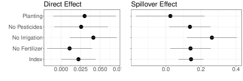
Figure 6: Regression estimates and $90\%$ confidence intervals (with standard errors clustered at the tehsil level) of regression of each outcome and of the index onto the treatment and share of treated individuals in the same tehsil with a linear specification.

Table 5: First table reports the regression of the absolute difference between the maximum temperature tomorrow predicted by the farmer and the forecast maximum temperature (first panel) or true maximum temperature (second panel). The second table reports the regression of whether the farmer incorrectly predicts rain. In parenthesis, standard errors clustered at the tehsil level.

	Dependent variable:
Incorrect beliefs about
	PxD forecast temperature			Real temperature
	(1)	(2)	(3)	(4)	(5)	(6)
Treatment	$-$0.698∗∗∗	$-$0.304	$-$0.469	$-$0.946∗∗∗	$-$0.783	$-$0.796
	(0.167)	(0.400)	(0.457)	(0.307)	(0.503)	(0.513)
Cluster Treat Prob	$-$0.906∗∗	$-$3.966∗∗∗	$-$0.490	0.746	$-$5.243∗∗∗	$-$0.930
	(0.413)	(1.123)	(2.203)	(1.083)	(1.366)	(2.211)
Cluster Treat Prob $\times$ Treatment		$-$0.662	$-$0.335		$-$0.180	$-$0.104
		(0.722)	(0.801)		(1.014)	(1.036)
Tehsil Fixed Effects	No	Yes	Yes	No	Yes	Yes
Time (month) Fixed Effects	No	No	Yes	No	No	Yes

	Dependent variable:
Incorrect beliefs about
	PxD forecast rain			Real rain
	(1)	(2)	(3)	(4)	(5)	(6)
Treatment	$-$0.008	$-$0.024	$-$0.016	$-$0.009	$-$0.035	$-$0.011
	(0.010)	(0.028)	(0.028)	(0.013)	(0.030)	(0.029)
Cluster Treat Prob	$-$0.051∗	$-$0.434∗∗∗	$-$0.228	0.014	$-$0.244∗∗	$-$0.144
	(0.030)	(0.060)	(0.141)	(0.036)	(0.102)	(0.203)
Cluster Treat Prob $\times$ Treatment		0.043	0.034		0.057	0.014
		(0.044)	(0.042)		(0.050)	(0.048)
Tehsil Fixed Effects	No	Yes	Yes	No	Yes	Yes
Time (month) Fixed Effects	No	No	Yes	No	No	Yes
Note:	∗p$<$0.1; ∗∗p$<$0.05; ∗∗∗p$<$0.01

6.4 Marginal effects, sequential experiment, and benefits

Next, we study the marginal effects on farmers’ correct beliefs about the rain that, as shown in the previous section, is a natural economic objective for the NGO since correct beliefs may correctly inform farming (e.g., irrigation) practices. We study marginal effects on beliefs about PxD forecasts (i.e., whether the farmer’s prediction agrees with PxD forecast) since these are less noisy and strongly correlate with real weather; see Table 4. In addition, Appendix C provides suggestive evidence that outcomes about correct beliefs do not exhibit treatment dynamics, formalizing the intuition that information about the weather one day may not affect future correct weather predictions in the upcoming weeks.

We estimate marginal effects using the first and second wave of the experiment. Figure 7 reports sample averages of farmers’ beliefs for clusters exposed to different treatment probabilities, pooling clusters into buckets whose treatment probability is $\beta\in\{0.4,0.5,0.6,0.7,0.8\}$, up to the small perturbation suggested in Section 3. The figure depicts the marginal effect at each point, estimated using information from the first wave for $\beta\in\{0.4,0.5,0.6\}$ and from the second wave for $\beta=0.7$. The figure also reports confidence intervals corresponding to $W(\beta)-W(0.8)$, after standardizing by the welfare value at $\beta=0.8$. Note that Figure 7 assumes no cluster fixed effects due to a lack of baseline outcomes. Although this is a strong assumption, it is motivated by the robustness of our findings as we control for tehsil-fixed effects in our parametric specification (Table 5), and districts (by design) and covariates’ balance across clusters (Table 2) (Table C.3 in Appendix C provides results for response rates for which we observe baseline outcomes).

Welfare at $\beta=0.8$ is significantly larger than welfare at $\beta=0.5$ to predict temperature and rainfall, as shown in Figure 7. However, effects for increasing $\beta=0.4$ to $\beta=0.5$ are near zero or non-significant. These results suggest that information diffusion occurs after “enough” individuals receive information (consistent with quasi-concave objectives studied in Appendix A.6). Namely, increasing treatments from $40\%$ to $50\%$ does not generate (significant) spillovers, while direct effects are small in magnitude (see Table 5).

Figure 7 provides suggestive evidence of decreasing marginal effects as $\beta$ approaches $0.8$. To test this hypothesis, we can test whether marginal effects at $\beta=0.6$ and $\beta=0.7$ are equal to zero. When predicting rain, we find that marginal effects at $\beta=0.6$ are statistically different from zero with a p-value of zero. Namely, we can reject the hypothesis that $W(\beta=0.55)-W(\beta=0.65)$ equal to zero. When instead we compare $W(0.6)$ to $W(0.8)$, the effects are smaller in magnitude and have a larger p-value (p-value 0.2). We also observe decreasing marginal effects for predicting maximum temperature for approaching $\beta=0.8$, although these are noisier (p-value 0.25 for marginal effects at $\beta=0.6$). These results suggest a phase transition after which marginal effects decrease (in absolute value). Treating $70\%$ to $80\%$ of individuals for information diffusion suffices.

Using the two experimental waves, we can estimate the welfare improvement of an adaptive experiment that, in the first wave, estimates the marginal effects at $\beta=0.6$, and in the second wave estimates marginal effects at $\beta=0.7$ as in Figure 7. Using predicted weather as a proxy for welfare, the two-wave experiment would recommend only treating $70\%$ to $80\%$ of the individuals. By assuming that zero marginal effects would persist after $\beta=0.8$, as Figure 7 would suggest, we can contrast this number with what a typical saturation experiment or grid search method would predict in Figure 8: a saturation experiment treating $\{0,50\%,100\%\}$ (Sinclair et al., 2012) of the individuals would not able to identify decreasing marginal effects near $70\%$, and similarly for other choices of treatment probabilities. Instead, it would recommend all individuals to be assigned to treatment. Our experiment uses information about the marginal effects to identify the optimum near $70\%$. In the first wave, the marginal effect was large and negative for both rain and temperature, suggesting increasing treatment probabilities, whereas in the second wave, the marginal effect for both rain and temperature at $\beta=0.7$ was close to zero. Treating $70\%$ to $80\%$ of individuals instead of $100\%$ would save approximately 0.29$ per farmer/year. This is economically significant if we consider a policy implemented on all farmers in Pakistan (approximately ten million), saving one million US dollars/year.

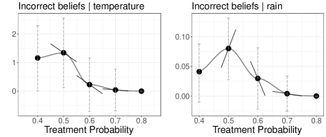
Figure 7: Incorrectly predicted maximum temperature (left-panel) and rain (right-panel) by the farmer and PxD for the day after the interview (rescaled by the correct predictions at $\beta=0.8$). Each of the first four dots reports the average effect by pooling observations around clusters with Low Saturation (first dot), and clusters with $\beta=\{0.4,0.5,0.6,0.7,0.8\}$, up to small perturbation $(\eta_{n}\leq 10\%)$. Confidence intervals report the $90^{th}$ and $10^{th}$ percentile for the welfare effects at each dot minus the welfare at $\beta=0.8$ and are computed via randomization inference. The lines report the estimated marginal effects.

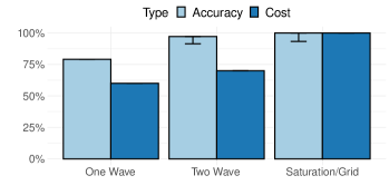
Figure 8: Benefits of a sequential experiment using predicted rain as a proxy for welfare. The light blue column reports the percentage change in average rain forecast accuracy (assuming forecast accuracy is constant after $\beta=0.8$; see right panel in Figure 7) generated by a policy recommendation using the proposed adaptive experiment, either with one-wave experiment (first column), or two waves (third column), and using a standard saturation experiment with probabilities $\{0,0.5,1\}$ (last column), relative to $W(0.8)$. Namely, the light blue bars report $(2W(0.8)-W(\beta))/W(0.8)$, where $\beta=0.6$ for One Wave and $\beta=0.7$ for Two Wave. The second, fourth, and sixth columns report the cost of the intervention that would be recommended by each of these experiments relative to the cost of treating everybody in the population. The policy-maker using only the first wave experiment deploys a policy that treats $60\%$ of the individuals, with corresponding costs of the intervention equal to $60\%$ of the total costs relative to treating everybody. The second wave experiment identifies positive marginal effects at $60\%$ and smaller and close to zero around $70\%$ and recommends treating around $70\%$ of the individuals. The forecast accuracy increases, as well as the costs of the total intervention. The standard saturation experiment does not identify marginal effects and recommends treating $100\%$ of the individuals. The error bars report $10\%$ confidence intervals over the improvement from the first to the second wave and from the two wave to treating everybody in the population (what Saturation/Grid would suggest). These are obtained via randomization inference on the gradient at $\beta=0.6$ and $\beta=0.7$, respectively, and using a first-order Taylor approximation to the welfare around $0.7$ for “Two Wave” and around $0.8$ for Saturation/Grid.

7 Calibrated numerical studies

We calibrate simulations to data from Cai et al. (2015) and Alatas et al. (2012, 2016) while making simplifying assumptions whenever necessary. In the first calibration, the outcome is insurance adoption, and the treatment is whether an individual received an intensive information session. In the second calibration, the treatment is whether a household received a cash transfer, and the outcome is program satisfaction. The experiment of Cai et al. (2015) contains multiple arms. Here, we only focus on the treatment effects of intensive information sessions, pooling the remaining arms together for simplicity. The experiment of Alatas et al. (2012) contains different arms assigned at the village level, as well as information on cash transfers assigned at the household level. Here, we study the effect of cash transfers only and control for village-level treatments when estimating the parameters of interest.

We study the problem of choosing a univariate $\beta$, which denotes the unconditional treatment probability. In each cluster $k$, we generate

$$Y_{i,t}=\phi_{0}+\phi_{1}D_{i,t}+\phi_{2}S_{i,t}+\phi_{3}S_{i,t}^{2}-cD_{i,t}+\eta_{i,t},\quad S_{i,t}=\frac{\sum_{j\neq i}A_{i,j}D_{i,t}}{\sum_{j\neq i}A_{i,j}},\eta_{i,t}\sim_{i.i.d.}\mathcal{N}(0,\sigma^{2}),$$ (20)

where $c$ is the cost of the treatment. We consider two sets of parameters $\Big{(}\phi_{0},\phi_{1},\phi_{2},\phi_{3},\sigma^{2}\Big{)}$ calibrated to data from Cai et al. (2015) and Alatas et al. (2012, 2016) respectively. We obtain information on neighbors’ treatment directly from data from Cai et al. (2015). For the second application, we merge data from Alatas et al. (2012), and Alatas et al. (2016), and use information from approximately 100 observations whose neighbors’ treatments are all observable to estimate the parameters. For either application, we estimate a linear model as in Equation (20), also controlling for additional covariates to guarantee the unconfoundedness of the treatment. We consider as cost of treatment $c=\phi_{1}$, i.e., the opportunity cost of allocating the treatment to a population of disconnected individuals.

We generate $K$ clusters, each with $N=600$ units, and sample $n\in\{200,400,600\}$. We generate a geometric network $A_{i,j}=1\Big{\{}||U_{i}-U_{j}||_{1}\leq 2\rho/\sqrt{N}\Big{\}},U_{i}\sim_{i.i.d.}\mathcal{N}(0,I_{2}),$ where the parameter $\rho$ governs the density of the network. The geometric formation process and the $1/\sqrt{N}$ follow similarly to simulations in Leung (2020). We report results for $\rho=2$ here, while results are robust for $\rho=6$ (denser network). The reader may refer to the online Appendix H for results with $\rho=6$. Throughout the analysis, without loss, we report welfare divided by its maximum $W(\beta^{*})$ (i.e., $W(\beta^{*})=1$), and we subtract the intercept $\phi_{0}$.

In Appendix D, we study the performance of the one-wave experiment. We show that the proposed test controls size uniformly across specifications and present desirable properties for power. Here, we present simulations for the multi-wave experiment. We fix the perturbation parameter $\eta_{n}=10\%$; similarly, in the adaptive experiment, we choose the learning rate $10\%/\sqrt{t}$ with gradient norm rescaling as Remark 9. Since the model does not allow for time-varying fixed effects, we estimate marginal effects without baseline outcomes. For the multi-wave experiment, we initialize parameters at a small treatment probability $\beta=0.2$.

We let $T\in\{5,10,15,20\}$. In Table 6, we report the welfare improvement of the proposed method with respect to a grid search method that samples observations from an equally spaced grid between $[0.1,0.9]$ with a size equal to the number of clusters (i.e., $2T$). We consider the best competitor between the one that maximizes the estimated welfare obtained from a correctly specified quadratic function and the one that chooses the treatment with the largest value within the grid. For both the competing methods, but not for the proposed procedure, we divide the outcomes’ variance $\sigma^{2}$ by $T$, simulating settings where researchers may sample outcomes $T$ times (hence outcomes with a lower variance) from each cluster before estimating treatment effects, and obtaining more precise information. The panel at the top of Table 6 reports the out-of-sample welfare improvement. The improvement is positive, and up to three percentage points for targeting information and up to sixty percentage points for targeting cash transfers. Improvements are generally larger for larger $T$. In one instance only, for $T=5$ and a small sample size $n=200$, we observe a negative effect for targeting information of two percentage points. The panel at the bottom of Table 6 reports positive and large improvements for the in-sample welfare across all the designs, worst-case across clusters. For the worst-case regret, we fix the number of clusters to $K=40$ for the proposed method and study the properties as a function of the number of iterations. The improvements are twice as large for targeting information and thirty percentage points larger for targeting cash transfers. These are often increasing in $T$ with a few exceptions since uniform concentration may deteriorate for large $T$ and small $n$ as we consider the worst-case welfare across clusters. In the online Appendices H.1, H.2, we report results across many other specifications of the network, policy functions, and choice of different parameters and different starting values (e.g., also when $\beta$ is initialized near the optimum).

Table 6: Multiple-wave experiment. $200$ replications. The relative improvement in welfare with respect to the best competitor for $\rho=2$. The panel at the top reports the out-of-sample regret, and the one at the bottom the worst-case in-sample regret.

	Information							Cash Transfer
$T=$	5	10	15	20					5	10	15	20
$n=200$	$0.057$	$0.135$	$0.297$	$0.212$					$0.232$	$0.243$	$0.264$	$0.287$
$n=400$	$0.226$	$0.209$	$0.355$	$0.346$					$0.243$	$0.274$	$0.321$	$0.335$
$n=600$	$0.299$	$0.281$	$0.344$	$0.492$					$0.261$	$0.313$	$0.343$	$0.360$
$n=200$	$0.621$	$0.731$	$0.736$	$0.752$					$0.247$	$0.279$	$0.300$	$0.320$
$n=400$	$0.652$	$0.745$	$0.874$	$0.898$					$0.266$	$0.306$	$0.343$	$0.352$
$n=600$	$0.646$	$0.801$	$0.942$	$1.125$					$0.294$	$0.360$	$0.387$	$0.387$

8 Conclusions

This paper makes two main contributions. First, it introduces a single-wave experimental design to estimate the marginal effect of the policy and test for policy optimality. The experiment also enables identifying and estimating treatment effects, which can be of independent interest. Second, it introduces an adaptive experiment to maximize welfare. We derive asymptotic properties for inference and provide a set of guarantees on the in-sample and out-of-sample regret. We illustrate the benefits of the method in a large-scale field experiment on information diffusion. Our empirical application shows that applications with “phase transitions”, i.e., when effects are constant after enough individuals receive the treatments, are natural scenarios where estimating marginal effects can be very informative.

This work opens new questions also from a theoretical perspective. We leave to future research the study of properties of the estimators when (i) clusters are not fully disconnected, in the spirit of Leung (2021); (ii) clusters need to be estimated, similarly to graph-clustering procedures; (iii) clusters present different distributions, as we discuss in Appendix A.4. Similarly, studying the properties of the proposed method, as the degree of interference is proportional to the sample size, is an interesting direction. This is theoretically possible, as illustrated in Theorem 3.1, and we leave its comprehensive analysis to future research. Finally, an open question is how to estimate policies when the network is only partially observed (e.g., Breza et al., 2020; Manresa, 2013), and how to measure costs and benefits of collecting network data, on which Section 5 provides novel directions for future research.

In this document we present main extensions, derivations, and additional algorithms. We collected an additional set of extensions that include staggered adoption, alternative network formation models, a rule of thumb for $\eta_{n}$ and additional numerical studies in online Appendices E - G available on the first author’s website and not for publication.

Appendix A Main extensions

A.1 Estimation with global interference

In this section, the treatment affects each unit in a cluster $k$ through a global interference mechanism mediated by a variable $p_{t}^{(k)}$. For simplicity, we let $X_{i}^{(k)}=1$.

Assumption A.1 (Global interference).

Let treatments be assigned as in Assumption 2.3. Let

$$Y_{i,t}^{(k)}=\alpha_{t}+\tau_{k}+g\Big{(}p_{t}^{(k)},\beta_{k,t}\Big{)}+\varepsilon_{i,t}^{(k)},\quad\mathbb{E}_{\beta_{k,1:t}}\Big{[}\varepsilon_{i,t}^{(k)}|p_{t}^{(k)}\Big{]}=0,$$

for some function $g(\cdot)$ unknown to the researcher, bounded and twice continuously differentiable with bounded derivatives, and unobservable $p_{t}^{(k)}$. Assume in addition that $\varepsilon_{i,t}^{(k)}\perp\varepsilon_{j\not\in\mathcal{I}_{i}^{(k)},t}^{(k)}|\beta_{k,1:t},p_{t}^{(k)}$ for some set $|\mathcal{I}_{i}^{(k)}|=\mathcal{O}(\gamma_{N})$.

Assumption A.1 states that the outcome within each cluster is a function of a common factor, and treatment assignment rule $\beta_{k,t}$.

Assumption A.2 (Global interference component).

Let treatments be assigned as in Assumption 2.3. Assume that $p_{t}^{(k)}=q(\beta_{k,t})+o_{p}(\eta_{n}),$ with $q(\beta)$ being unknown, bounded and twice continuously differentiable in $\beta$ with uniformly bounded derivatives.

Assumption A.2 states that the factor can be expressed as the sum of two components. The first component $q(\cdot)$ depends on the policy parameter $\beta_{k,t}$ assigned at time $t$ and on the distribution of covariates of all units in a cluster. The second component is a stochastic component that depends on the realized treatment effects. We illustrate an example below.

Example A.1 (Within cluster average).

Suppose that $Y_{i,t}^{(k)}=t(\bar{D}_{t}^{(k)},\nu_{i,t}),\nu_{i,t}^{(k)}\sim_{i.i.d.}\mathcal{P}_{\nu},D_{i,t}^{(k)}\sim_{i.i.d.}\mathrm{Bern}(\beta)$ where $t(\cdot)$ is some arbitrary (smooth) function. Then $p_{t}^{(k)}=\bar{D}_{t}^{(k)}$ i.e., individuals depend on the average exposure in a cluster. We can write $Y_{i,t}^{(k)}=t(p_{t}^{(k)},\nu_{i,t}^{(k)})$ where $p_{t}^{(k)}=\beta+(\bar{D}_{t}^{(k)}-\beta),$ which satisfies Assumption A.2 for $\eta_{n}=n^{-1/3}$ or larger. ∎

We are interested in $M_{g}(\beta)=\frac{\partial W_{g}(\beta)}{\partial\beta},W_{g}(\beta)=g(q(\beta),\beta).$ Estimation of the marginal effect follows similarly to Equation (7). The following theorem guarantees consistency.

Theorem A.1.

Let Assumption A.1, A.2 hold with subgaussian $\varepsilon_{i,t}^{(k)}$, $X_{i}=1$. For $\widehat{M}_{(k,k+1)}$ as in Algorithm 2, for $k$ being odd: $\Big{|}\widehat{M}_{(k,k+1)}-M_{g}(\beta)\Big{|}=\mathcal{O}_{p}\left(\sqrt{\frac{\gamma_{N}\log(n\gamma_{N})}{\eta_{n}^{2}n}}+\eta_{n}\right)+o_{p}(1).$

The proof is in Appendix B.3.

A.2 Policy choice with dynamic treatments

This section studies an experimental design with carry-overs occur. Let $X_{i}=1$ for simplicity.

Assumption A.3 (Dynamic model).

For treatments assigned with exogenous parameters $(\beta_{k,1},\cdots,\beta_{k,t})$ as in Assumption 2.3, let $Y_{i,t}^{(k)}=\Gamma(\beta_{t},\beta_{t-1})+\varepsilon_{i,t}^{(k)},\mathbb{E}_{\beta_{k,1:t}}\Big{[}\varepsilon_{i,t}^{(k)}\Big{]}=0,$ for some unknown $\Gamma(\cdot)$, $\varepsilon_{i,t}^{(k)}$.

The components $\beta_{k,t},\beta_{k,t-1}$ capture present and carry-over effects that result from individual and neighbors’ treatments in the past two periods. We estimate a path of policies $(0,\beta_{1},\cdots,\beta_{T})$ from an experiment, where, in the first period, we assume for simplicity that none of the individuals is treated. This path is then implemented on a new population.

Example A.2.

Suppose that $Y_{i,t}^{(k)}=D_{i,t}^{(k)}\phi_{1}+\frac{\sum_{j=1}^{n}A_{i,j}^{(k)}D_{i,t-1}}{\sum_{j=1}^{n}A_{i,j}^{(k)}}\phi_{2}+\nu_{i,t}^{(k)},D_{i,t}^{(k)}\sim_{i.i.d.}\mathrm{Bern}(\beta_{t}).$ Let $\nu_{i,t}$ be a zero-mean random variable. The expression simplifies to $Y_{i,t}^{(k)}=\beta_{t}\phi_{1}+\beta_{t-1}\phi_{2}+\varepsilon_{i,t}^{(k)}$ where $\varepsilon_{i,t}^{(k)}$ is zero mean, and depends on neighbors’ and individual assignments. ∎

Given an horizon $T^{*}$, define the long-run welfare as follows: $\mathcal{W}(\{\beta_{s}\}_{s=1}^{T^{*}})=\sum_{t=1}^{T^{*}}q^{t}\Gamma(\beta_{t},\beta_{t-1}),$ for a known discounting factor $q<1$, where $\beta_{0}=0$. The long-run welfare deifines the cumulative (discounted) welfare obtained from a certain sequence of decisions $(\beta_{1},\beta_{2},\cdots)$. The goal is to maximize the long-run welfare.

The choice of future treatment probabilities must depend on the ones chosen in the past. We parametrize future treatment probabilities based on past treatment probabilities as follows $\beta_{t+1}=h_{\theta}(\beta_{t},\beta_{t-1}),\theta\in\Theta.$ The parametrization is imposed for computational convenience. The choice of letting $\beta_{t+1}$ be a function of the past two $(\beta_{t},\beta_{t-1})$ only follows from the first order conditions with respect to $\beta_{t+1}$. For some arbitrary large $T^{*}$, the objective function takes the following form

$$\widetilde{W}(\theta) =\sum_{t=1}^{T^{*}}q^{t}\Gamma\Big{(}\beta_{t},\beta_{t-1}\Big{)},\quad\beta_{t}=h_{\theta}(\beta_{t-1},\beta_{t-2})\quad\text{ for all }t\geq 1,\quad\beta_{0}=\beta_{-1}=0.$$ (A.1)

Here $\widetilde{W}(\theta)$ denotes the long-run welfare indexed by a given policy’s parameter $\theta$. The objective function defines the discounted cumulative welfare induced by the policy $h_{\theta}$.

Algorithm E.3 estimates the function $\Gamma(\cdot)$ using a single wave experiment. It then uses the estimated function $\Gamma(\cdot)$ and its gradient to estimate the welfare-maximizing parameter $\theta$. Specifically, we conduct the randomization using two periods of experimentation only. We partition the space $[0,1]^{2}$ into a grid $\mathcal{G}$ of equally spaced components $(\beta_{1}^{r},\beta_{2}^{r})$ for each triad of clusters $r$. Within each triad, we induce small deviations to the parameters $\beta$. For each triad $r$, the algorithm returns $\widetilde{\Gamma}(\beta_{2}^{r},\beta_{1}^{r}),\widehat{g}_{1}(\beta_{2}^{r},\beta_{1}^{r}),\widehat{g}_{2}(\beta_{2}^{r},\beta_{1}^{r})$ where the latter two components are the estimated partial derivatives of $\Gamma(\cdot)$, and $\widetilde{\Gamma}(\beta_{2}^{r},\beta_{1}^{r})$ is the within cluster average.

For each pair of parameters $(\beta_{2},\beta_{1})$, we estimate $\widehat{\Gamma}(\beta_{2},\beta_{1})$ as follows

$$\widehat{\Gamma}(\beta_{2},\beta_{1})=\widetilde{\Gamma}(\beta_{2}^{r},\beta_{1}^{r})+\widehat{g}_{2}(\beta_{2}^{r},\beta_{1}^{r})(\beta_{2}-\beta_{2}^{r})+\widehat{g}_{1}(\beta_{2}^{r},\beta_{1}^{g})(\beta_{1}-\beta_{1}^{r}),$$ (A.2)

$$\text{ where }\quad(\beta_{1}^{r},\beta_{2}^{r})=\mathrm{arg}\min_{(\tilde{\beta}_{1},\tilde{\beta}_{2})\in\mathcal{G}}\Big{\{}||\beta_{1}-\tilde{\beta}_{1}||^{2}+||\beta_{2}-\tilde{\beta}_{2}||^{2}\Big{\}}.$$

we estimate $\Gamma(\beta_{2},\beta_{1})$ at $(\beta_{2},\beta_{1})$ using a a first-order Taylor approximation around the closest pairs of parameters in the grid $\mathcal{G}$. Given $\widehat{\Gamma}$, we estimate the welfare-maximizing parameter

$$\widehat{\theta}\in\mathrm{arg}\max_{\theta\in\Theta}\sum_{t=1}^{T^{*}}q^{t}\widehat{\Gamma}(\beta_{t},\beta_{t-1}),\quad\beta_{t}=h_{\theta}(\beta_{t-1},\beta_{t-2})\quad\forall t\geq 1,\quad\beta_{0}=\beta_{-1}=0.$$

In the following theorem, we study the out-of-sample regret.

Theorem A.2 (Out-of-sample regret).

Let Assumption A.3 hold. Let $X=1$, and suppose that $\Gamma(\beta_{2},\beta_{1})$ is twice differentiable with bounded derivatives. Let treatments be assigned as in Algorithm E.3. Suppose in addition that $\varepsilon_{i,t}^{(k)}\perp\varepsilon_{j\not\in\mathcal{I}_{i}^{(k)}}^{(k)}$ where $|\mathcal{I}_{i}^{(k)}|\leq\gamma_{N}$, for some arbitrary $\gamma_{N}$ and $\varepsilon_{i,t}^{(k)}$ is sub-gaussian. Let $\gamma_{N}\log(\gamma_{N})/(\eta_{n}^{2}n)=o(1)$. Then $\lim_{n\rightarrow\infty}P\Big{(}\sup_{\theta\in\Theta}\widetilde{W}(\theta)-W(\widehat{\theta})\leq\frac{\bar{C}}{K}\Big{)}=1$ for a constant $\bar{C}$ independent of $K$.

The proof is in Appendix B.4. To our knowledge, Algorithm E.3 is novel to the literature of experimental design.

Theorem A.2 shows that the regret scales at a rate $1/K$. The key insight is to use information of the estimated gradient. Different from previous sections, the rate $1/K$ is specific to the one-dimensional setting and carry-overs over two consecutive periods. In $p$ dimensions, the rate would be of order $1/K^{2/(p+1)}$ due to the curse of dimensionality.

A.3 Non-adaptive experiment with local perturbations

This sub-section serves two purposes. First, it sheds light on comparisons of the adaptive procedure with grid-search-type methods, showing drawbacks of the grid-search approach in terms of convergence of the regret. Second, it shows how, when an adaptive procedure is not available, we can still use information from the marginal effect estimated as we propose in Algorithm 1, to improve convergence rates in $K$.

The algorithm that we propose is formally discussed in Algorithm E.1 and works as follows. First, we construct a fine grid $\mathcal{G}$ of the parameter space $\mathcal{B}$ (with $p$ dimensions), with equally spaced parameters. Second, we pair clusters, and assign a different parameter $\beta^{k}$ for each pair $(k,k+1)$ from the grid $\mathcal{G}$. Third, in each pair, we estimate the gradient $\widehat{M}_{(k,k+1)}\in\mathbb{R}^{p}$, by perturbing, sequentially for $T=p$ periods, one coordinate at a time of the parameter $\beta^{k}$. we estimate welfare using a first-order Taylor expansion

$$\widehat{W}(\beta)=\bar{W}^{k^{*}(\beta)}+\widehat{M}_{(k^{*}(\beta),k^{*}(\beta)+1)}^{\top}(\beta-\beta^{k^{*}(\beta)}),\quad\hat{\beta}^{ow}=\mathrm{arg}\max_{\beta\in\mathcal{B}}\widehat{W}(\beta),$$ (A.3)

$$\text{where }k^{*}(\beta)=\mathrm{arg}\min_{k\in\{1,3,\cdots,K-1\},\beta^{k}\in\mathcal{G}}||\beta^{k}-\beta||^{2},\quad\bar{W}^{k}=\frac{1}{2}\Big{[}\frac{1}{T}\sum_{t=1}^{T}\bar{Y}_{t}^{k}-\bar{Y}_{0}^{k}+\frac{1}{T}\sum_{t=1}^{T}\bar{Y}_{t}^{k+1}-\bar{Y}_{0}^{k+1}\Big{]}.$$

Here, $\bar{Y}_{t}^{k}$ is the average outcome in cluster $k$ at time $t$, and $\widehat{M}_{(k^{*},k^{*}+1)}$ is estimated as in Algorithm E.1. We can now characterize guarantees as $n\rightarrow\infty$, and $K,p<\infty$.

Theorem A.3.

Suppose that $\varepsilon_{i,t}^{(k)}$ is sub-gaussian. Let Assumptions 2.1, 2.2, 3.1, and $\eta_{n}=o(n^{-1/4})$, $\gamma_{N}\log(n\gamma_{N}K)/(\eta_{n}^{2}n)=o(1)$. Consider $\hat{\beta}^{ow}$ as in Algorithm E.1, with $\mathcal{B}\subseteq[0,1]^{p}$. For a constant $\bar{C}<\infty$ independent of $(n,T,K)$, $\lim_{n\rightarrow\infty}P\left(W(\beta^{*})-W(\hat{\beta}^{ow})\leq\frac{\bar{C}}{K^{2/p}}\right)=1.$

The proof is in Appendix B.5. Theorem A.3 showcases two properties of the method. First, for $p=1$, the rate of convergence is of order $1/K^{2}$, which is possible because we also estimate and leverage the gradient $\widehat{M}$. The insight is to augment the estimator of the welfare with $\widehat{M}$, since, otherwise, the rate would be slower in $K$. One drawback of a grid search approach is that, as $p>1$, the method suffers a curse of dimensionality, and the rate in $K$ decreases as $p$ increases. This is different from the adaptive procedure (e.g., Corollary 4), where the rate in $K$ does not depend on $p$. A second disadvantage of the grid search is that the method does not control the in-sample regret, formalized below.

Proposition A.4 (Non-vanishing in-sample regret).

There exists a strongly concave $W(\cdot)$, such that, for $p=1$, $W(\beta^{*})-\frac{1}{K}\sum_{k=1}^{K}W(\beta^{k})\geq c,$ for $c>0$ independent of $(n,K,T)$.

Proof of Proposition A.4.

By concavity, $W(\beta^{*})-\frac{1}{K}\sum_{k=1}^{K}W(\beta^{k})\geq W(\beta^{*})-W(\frac{1}{K}\sum_{k=1}^{K}\beta^{k})=W(\beta^{*})-W(0.5),$ which completes the proof, for a suitable choice of $W(\cdot)$. ∎

A.4 Pairing clusters with heterogeneity

A.4.1 Inference and estimation with observed cluster heterogeneity

In this subsection, we discuss an extension to allow for cluster heterogeneity. Consider $\theta_{k}\in\Theta$ to denote the cluster’s type for cluster $k$, where $\Theta$ is a finite space (i.e., there are finitely many cluster types). Let $\theta_{k}$ be observable by the researcher and be non-random .

Assumption A.4.

For each cluster $k$, Assumption 2.1 holds, with $F_{X},F_{U|X}$ replaced by $F_{X}(\theta_{k}),F_{U|X}(\theta_{k})$ functions of $\theta_{k}$; Assumption 2.2 holds with $r(\cdot)$ that also depends on $\theta_{k}$.

Assumption A.4 allows for both the distribution of covariates and unobservables and potential outcomes to also depend on the cluster’s type $\theta_{k}$.

Lemma A.5.

Under Assumption A.4, under an assignment in Assumption 2.3, for some function $y(\cdot)$ unknown to the researcher,

$$Y_{i,t}^{(k)}=y\Big{(}X_{i}^{(k)},\beta_{k,t},\theta_{k}\Big{)}+\varepsilon_{i,t}^{(k)}+\alpha_{t}+\tau_{k},\quad\mathbb{E}_{\beta_{k,t}}\Big{[}\varepsilon_{i,t}^{(k)}|X_{i}^{(k)}\Big{]}=0.$$ (A.4)

Different from Lemma 2.1, here the the functions also depend on the cluster’s type $\theta_{k}$. The proof of Lemma A.5 follows verbatim from the one of Lemma 2.1, taking here into account also the (deterministic) cluster’s type.

Single wave experiment

In the context of a single-wave experiment, we are interested in testing the null hypothesis of whether a class of decisions $\beta(\theta),\theta\in\Theta$, which depends on the cluster’s type, is optimal. Namely, let $W\Big{(}\beta(\theta),\theta\Big{)}=\int y(x,\beta(\theta),\theta)dF_{X}(\theta),\quad\beta:\Theta\mapsto\mathcal{B},\quad\theta\in\Theta$ be the welfare corresponding to cluster’s type $\theta$, for a decision rule $\beta(\theta)$. Also, let $M\Big{(}\beta(\theta),\theta\Big{)}=\frac{\partial W(b,\theta)}{\partial b}\Big{|}_{b=\beta(\theta)}$ be the marginal effect with respect to changing $\beta(\theta)$ (for fixed $\theta$). The null hypothesis is $H_{0}:M\Big{(}\beta(\theta),\theta\Big{)}=0,\forall\theta\in\Theta,$ i.e., the (baseline) policy $\beta(\theta)$ is optimal for all clusters under consideration. The algorithm follows similarly to Algorithm 2 with the following modification: instead of matching arbitrary clusters, we construct pairs such that elements in the same pair $(k,k+1)$ are such that $\theta_{k}=\theta_{k+1}$.

Multi-wave experiment

For the multi-wave experiment, our goal is to find $\beta^{*}(\theta)$ such that $\beta^{*}(\theta)\in\mathrm{arg}\max_{b\in\mathcal{B}}W(b,\theta),\forall\theta\in\Theta.$ Similarly to the single-wave experiment, clusters $(k,k^{\prime})$ of the same type $\theta_{k}=\theta_{k^{\prime}}$ are first matched together. We can then consider two extensions. The first extension consists of grouping clusters of the same type together, estimating separately $\beta^{*}(\theta)$ for each $\theta\in\Theta$. In this case the regret bound holds up-to a factor of order $\min_{t}P(\theta=t)$, with $P(\theta=t)$ denoting the (exact) share of clusters of type $t$. The second approach instead consists of updating the same policy from a given pair using information from that same pair. The validity of this latter extension relies on time independence.

A.4.2 Matching clusters with distributional embeddings

Next, we turn to settings where covariates have different distributions in different clusters. Let $X_{i}^{(k)}\sim_{i.i.d.}F_{X}^{(k)},$ with $F_{X}^{(k)}$ being cluster-specific. Treatments are assigned as follows

$$t=0: D_{i,0}^{(h)}\sim\pi(X_{i}^{(h)};\beta_{0}),\quad h\in\{k,k^{\prime}\}$$ (A.5)

$$t=1: D_{i,1}^{(k)}\sim\pi(X_{i}^{(k)};\beta),\quad D_{i,1}^{(k^{\prime})}\sim\pi(X_{i}^{(k^{\prime})};\beta^{\prime}).$$

The estimand and estimator are respectively

$$\omega_{k} =\int y(x;\beta)dF_{X}^{(k)}(x)-\int y(x;\beta^{\prime})dF_{X}^{(k)}(x),\quad\widehat{\omega}_{k}(k^{\prime})=\Big{[}\bar{Y}_{1}^{(k)}-\bar{Y}_{1}^{(k^{\prime})}\Big{]}-\Big{[}\bar{Y}_{0}^{(k)}-\bar{Y}_{0}^{(k^{\prime})}\Big{]}.$$

our focus is to control the bias of the estimator via matching.

Lemma A.6.

Let Assumption 2.1, 2.2, and treatments assigned as in Equation (A.5). Then

$$\mathbb{E}[\widehat{\omega}_{k}(k^{\prime})]-\omega_{k}=\int\Big{(}y(x;\beta^{\prime})-y(x;\beta_{0})\Big{)}d\Big{(}F_{X}^{(k)}(x)-F_{X}^{(k^{\prime})}(x)\Big{)}.$$

Lemma A.6 shows the bias depends on the difference between the expectations averaged over two different distributions. The bias is unknown since it depends on the function $y(\cdot)$, which is not identifiable with finitely many clusters. We therefore bound the worst-case error over a class of functions $x\mapsto[y(x;\beta^{\prime})-y(x;\beta_{0})]\in\mathcal{M}$, with $\mathcal{M}$ defined below.

We start by defining $\mathcal{M}$ be a reproducing kernel Hilbert space (RKHS) equipped with a norm $||\cdot||_{\mathcal{M}}$. Without loss of generality, we study the worst-case functionals over the unit-ball. Formally, we focus on bounding the worst-case error of the form

$$\sup_{[y(\cdot;\beta^{\prime})-y(\cdot;\beta_{0})]\in\mathcal{M}:||y(\cdot;\beta^{\prime})-y(\cdot;\beta_{0})||_{\mathcal{M}}\leq 1}\Big{|}\omega_{k}-\mathbb{E}[\widehat{\omega}_{k}(k^{\prime})]\Big{|}=\sup_{f\in\mathcal{M}:||f||_{\mathcal{M}}\leq 1}\Big{\{}\int f(x)d(F_{X}^{(k)}-F_{X}^{(k^{\prime})})\Big{\}}.$$ (A.6)

The right-hand side is know as the maximum mean discrepancy (MMD), a measure of distances in RKHS (see Muandet et al., 2016, and references therein). It is known that the MMD can be consistently estimated using kernels. In particular, given a particular choice of a kernel $k(\cdot)$, which corresponds to a certain RKHS, we can estimate

$$\widehat{\mathrm{MMD}}^{2}(k,k^{\prime}) =\frac{1}{n(n-1)}\sum_{i=1}^{n}\sum_{j\neq i}h\Big{(}X_{i}^{(k)},X_{i}^{(k^{\prime})},X_{j}^{(k)},X_{j}^{(k^{\prime})}\Big{)},$$ (A.7)

$$h(x_{i},y_{i},x_{j},y_{j}) =k(x_{i},x_{j})+k(y_{i},y_{j})-k(x_{i},y_{j})-k(x_{j},y_{i}).$$

Consistency follows from results discussed in Muandet et al. (2016).

We now turn to the problem of matching clusters. The following matching algorithm is considered: (i) construct $k^{\prime}\in\mathrm{arg}\min_{k\neq k}\widehat{\mathrm{MMD}}^{2}(k,k^{\prime}).$ based on the minimum estimated MMD in Equation (A.7); (ii) randomize treatments as in Equation (A.5); (iii) estimate $\widehat{\omega}_{k}(k^{\prime})$. With many clusters, we suggest minimizing the average MMD over cluster pairs.

A.5 Tests with a $p$-dimensional vector of marginal effects

In the following lines we extend Algorithm 2 to testing the following null $H_{0}:M^{(j)}(\beta)=0,\text{ for some }p\geq p_{1}\geq 1,$ where we consider a generic number of dimensions tested $p_{1}$.

Algorithm A.1 One wave experiment for inference

1:Value $\beta\in\mathbb{R}^{p}$, $K$ clusters, $2$ periods of experimentation, number of tests $t$.

2:Match clusters into pairs $K/2$ pairs with consecutive indexes $\{k,k+1\}$;

3:$t=0$ (baseline):

4:a: Treatments are assigned at some baseline $\beta_{0}$ $D_{i,0}^{(h)}\sim\pi(X_{i}^{(h)},\beta_{0}),h\in\{1,\cdots,K\}$.

5:b: Collect baseline values: for $n$ units in each cluster observe $Y_{i,0}^{(h)},h\in\{1,\cdots,K\}$.

6:$t=1$ (experimentation-wave)

7:Assign each pair of clusters $\{k,k+1\}$ to a coordinate $j\in\{1,\cdots,p\}$ (with the same number of pairs to each coordinate)

8:For each pair $\{k,k+1\}$, $k$ is odd, assigned to coordinate $j$

9:a: Randomize

$$D_{i,1}^{(h)}\sim\begin{cases}&\pi(X_{i}^{(h)},\beta+\eta_{n}\underline{e}_{j})\text{ if }h=k\\ &\pi(X_{i}^{(h)},\beta-\eta_{n}\underline{e}_{j})\text{ if }h=k+1\end{cases},\quad n^{-1/2}<\eta_{n}\leq n^{-1/4}$$

10:b: For $n$ units in each cluster $h\in\{k,k+1\}$ observe $Y_{i,1}^{(h)}$.

11:c: Estimate the marginal effect for coordinate $j$ as $\widehat{M}_{k}=\frac{1}{2\eta_{n}}\Big{[}\bar{Y}_{1}^{(k)}-\bar{Y}_{0}^{(k)}\Big{]}-\frac{1}{2\eta_{n}}\Big{[}\bar{Y}_{1}^{(k+1)}-\bar{Y}_{0}^{(k+1)}\Big{]}$ return $\widetilde{M}_{n}=\Big{[}\widehat{M}_{1},\widehat{M}_{3},\cdots,\widehat{M}_{K-1}\Big{]}$.

we define $\mathcal{K}_{j}$ the set of pairs in Algorithm A.1 used to estimate the $j^{th}$ entry of $M(\beta)$. Define $\bar{M}_{n}^{(j)}=\frac{2p_{1}}{K}\sum_{k\in\mathcal{K}_{j}}\widehat{M}_{k},$ the average marginal effect for coordinate $j$ estimated from those clusters is used to estimate the effect of the $j^{th}$ coordinate. we construct

$$Q_{j,n}=\frac{\sqrt{K/(2p_{1})}\bar{M}_{n}^{(j)}}{\sqrt{(K/(2p_{1})-1)^{-1}\sum_{k\in\mathcal{K}_{j}}(\widehat{M}_{k}^{(j)}-\bar{M}_{n}^{(j)})^{2}}},\quad\mathcal{T}_{n}=\max_{j\in\{1,\cdots,p_{1}\}}|Q_{j,n}|,$$ (A.8)

where $\mathcal{T}_{n}$ denotes the test statistics. The proposed test-statistic is particularly suited when a large deviation occurs over one dimension of the vector.

Theorem A.7 (Nominal coverage).

Let Assumptions 2.1, 2.2, 3.2 hold. Let $n^{1/4}\eta_{n}=o(1),\gamma_{N}^{2}/N^{1/4}=o(1)$, $K<\infty$. Let $K\geq 4p_{1}$, $H_{0}$ be as defined in Equation (8). For any $\alpha\leq 0.08$, $\lim_{n\rightarrow\infty}P\Big{(}\mathcal{T}_{n}\leq q_{\alpha}\Big{|}H_{0}\Big{)}\geq 1-\alpha,\text{ where }q_{\alpha}=\mathrm{cv}_{K/(2l)-1}\Big{(}1-(1-\alpha)^{1/p_{1}}\Big{)},$ with $\mathrm{cv}_{K/(2l)-1}(h)$ denotes the critical value of a two-sided t-test with level $h$ with test-statistic having $K/(2p_{1})-1$ degrees of freedom.

The proof is in Appendix B.6.

A.6 Out-of-sample regret with strict quasi-concavity

In the following lines, we provide guarantees on the regret bounds for the adaptive algorithm in Section 4 under quasi-concavity. We replace Assumption 4.2 with the following condition.

Assumption A.5 (Local strong concavity and strict quasi-concavity).

Assume that the following conditions hold: (A) For every $\beta,\beta^{\prime}\in\mathcal{B}$, such that $W(\beta^{\prime})-W(\beta)\geq 0$, then $M(\beta)^{\top}(\beta^{\prime}-\beta)\geq 0;$ (B) For every $\beta\in\mathcal{B}$, $||M(\beta)||_{2}\geq\mu||\beta-\beta^{*}||_{2}$, for a positive constant $\mu>0$; (C) $W(\beta)$ is $\sigma$-strongly concave at $\beta^{*}$ (but not necessarily for $\beta\neq\beta^{*}$), with $\beta^{*}\in\tilde{\mathcal{B}}\subset\mathcal{B}$ being in the interior of $\mathcal{B}$.

Condition (A) imposes a quasi-concavity of the objective function. Condition (B) assumes that the marginal effect only vanishes at the optimum, ruling out regions over which marginal effects remain constant at zero. A notion of strict quasi-concavity can be found in Hazan et al. (2015). Condition (C) imposes strong concavity locally at $\beta^{*}$ but not necessarily globally. The choice of the learning rate consists of a gradient norm rescaling, as discussed in Remark 9.

Theorem A.8.

Let Assumptions 2.1, 2.2, 4.1, A.5 hold. Consider a learning rate $\alpha_{k,w}$ as in Equation (17), for arbitrary $v\in(0,1)$, and $\epsilon_{n}$ such that $\epsilon_{n}\geq\sqrt{p}\Big{[}\bar{C}\sqrt{\gamma_{N}\frac{\log(\gamma_{N}\check{T}K/\delta)}{\eta_{n}^{2}n}}+\eta_{n}\Big{]},\quad\frac{1}{4\mu\check{T}^{1/2-v/2}}-\epsilon_{n}\geq 0.$ Take a small $1/4>\xi>0$, and let $n^{1/4-\xi}\geq\bar{C}\sqrt{\log(n)p\gamma_{N}T^{2}e^{BpT}\log(KT)}$, $\eta_{n}=1/n^{1/4+\xi}$, for finite constants $\infty>B,\bar{C}>0$. Then, for $T\geq\zeta^{1/v}$, for a finite constant $\zeta<\infty$, there exists a sufficiently small and finite $\kappa>0$ in Equation (17) such that with probability at least $1-1/n$, $W(\beta^{*})-W(\hat{\beta}^{*})=\mathcal{O}(\check{T}^{-1+v}).$

The proof of Theorem A.8 leverages properties of gradient descent with gradient norm rescaling in Hazan et al. (2015), together with concentration bounds similar to those obtained to derive Theorem 4.2. The rate obtained differs from Theorem 4.2 in two aspects: it is of order $T^{-1+v}$ for arbitrary small $v$ instead of $T^{-1}$ and the sample size grows exponentially instead of polynomially in $T$. The reason for the first is to control the inverse gradient when close to zero, and the reason for the second is due to the different learning rate which does not divide by $1/t$ (see the proof of Lemma B.9 for details).

A.7 Non separable fixed effects

In the following lines, we show how we can leverage direct and marginal spillover effects to identify the marginal effects when fixed effects are non-separable in time and cluster identity.

Theorem A.9 (Marginal effects with non-separable fixed effects).

Let $X=1$, and suppose that $m(d,1,\beta)$ is bounded and twice differentiable with bounded derivatives for $d\in\{0,1\}$. Let Assumptions 2.1 hold. Suppose that fixed-effects are non-separable, with

$$Y_{i,t}^{(k)}=m(D_{i,t}^{(k)},1,\beta)+\alpha_{k,t}+\varepsilon_{i,t}^{(k)},\quad\mathbb{E}[\varepsilon_{i,t}^{(k)}]=0,\quad D_{i,t}^{(k)}\sim_{i.i.d.}\mathrm{Bern}(\beta),$$

and $m(1,1,\beta)$ being a constant function in $\beta$. Then

$$\mathbb{E}\Big{[}\hat{\Delta}_{k}(\beta)+\hat{S}(0,\beta)(1-\beta)-(1-\beta)\hat{S}(1,\beta)\Big{]}=M(\beta)+\mathcal{O}(\eta_{n}).$$

The proof is in Appendix B.7. Theorem A.9 shows that we can use the information on the spillover and direct treatment effects to identify the marginal effects in the presence of non-separable time and cluster fixed effects. The theorem leverages the assumption that spillovers only occur on the control individuals but not the treated. The assumption of lack of spillovers on the treated may hold in some (e.g Duflo et al., 2023) but not all settings.

A.8 Permutation tests

For permutation tests, consider the vectors

$$V_{1}=\begin{bmatrix}&\bar{Y}_{1}^{(1)}-\bar{Y}_{0}^{(1)}\\ &\bar{Y}_{1}^{(3)}-\bar{Y}_{0}^{(3)}\\ &\vdots\\ &\bar{Y}_{1}^{(K-1)}-\bar{Y}_{0}^{(K-1)}\end{bmatrix},\quad V_{2}=\begin{bmatrix}&\bar{Y}_{1}^{(2)}-\bar{Y}_{0}^{(2)}\\ &\bar{Y}_{1}^{(4)}-\bar{Y}_{0}^{(4)}\\ &\vdots\\ &\bar{Y}_{1}^{(K)}-\bar{Y}_{0}^{(K)}.\end{bmatrix}$$

We consider permutation tests over the sign of $\tilde{V}_{s}=s(V_{1}-V_{2}),s\in\{-1,1\}^{K/2}$. We define $T(\tilde{V}_{s})$ the t-static obtained from the vector $\tilde{V}_{s}$, and $C_{K}^{P}(\alpha)$ the $(1-\alpha)^{th}$ quantile of $|T(\tilde{V}_{s})|,s\in\{-1,1\}^{K/2}$ (up-to rounding). From Theorem 3.2, the distribution of $T(\tilde{V}_{s})$ is invariant under the null hypothesis.

It is possible to consider alternative t-statistics or permutations e.g., also permuting over the pairs’ assignments. We omit this for brevity

Appendix B Derivations

First, we introduce conventions and notation. we say that $x\lesssim y$ if $x\leq cy$ for a positive constant $c<\infty$. For $K$ many clusters, we say that $\lfloor k\rceil=k1\{K\leq k\}+(k-K)1\{k>K\}$. we will refer to $\widehat{M}_{(k,k+1)}$ as $\widehat{M}_{k}$ for $k$ is odd for short of notation. Also, we define $\check{M}_{k,s}=\widehat{M}_{\lfloor k+2\rceil,s}$. The following definition introduces the notion of a dependency graph (Janson, 2004).

Definition B.1 (Dependency graph).

For given random variables $R_{1},\cdots,R_{n}$, $W_{n}\in\{0,1\}^{n\times n}$ is a non-random matrix defined as dependecy graph of $(R_{1},\cdots,R_{n})$ if, for any $i$, $R_{i}\perp R_{j:W_{n}^{(i,j)}=0}$. we denote the dependency neighbors $N_{i}=\{j:W_{n}^{(i,j)}=1\}$. ∎

Definition B.2 (Cover).

Given an adjacency matrix $A_{n}$, with $n$ rows and columns, a family $\mathcal{C}_{n}=\{\mathcal{C}_{n}(j)\}_{j}$ of disjoint subsets of $\{1,\cdots,n\}$ is a proper cover of $A_{n}$ if $\cup_{j}\mathcal{C}_{n}(j)=\{1,\cdots,n\}$ and $\mathcal{C}_{n}(j)$ contains units such that for any pair of elements $\{i,k\in\mathcal{C}_{n}(j)\}$, $A_{n}^{(i,k)}=0$. ∎

Namely, a proper cover of $A_{n}$ defines a set of disjoint sets, where each disjoint set contains some indexes of units that are not neighbors in $A_{n}$. Note that a proper cover always exists, since, if $A_{n}$ is fully connected, then the number of disjoint sets is just $n$, one for each element.

The size of the smallest proper cover is the chromatic number, defined as $\chi(A_{n})$.

Definition B.3 (Chromatic number).

The chromatic number $\chi(A_{n})$, denotes the size of the smallest proper cover of $A_{n}$. ∎

We define the oracle descent procedure absent of sampling error. Let $\beta\in\mathcal{B}=[\mathcal{B}_{1},\mathcal{B}_{2}]^{p}$, where $\mathcal{B}_{1},\mathcal{B}_{2}$ are finite. Also, let $P_{\mathcal{B}_{1},\mathcal{B}_{2}}$ be the projection operator onto $\mathcal{B}$.

Definition B.4 (Oracle gradient descent under strong concavity).

We define, for $\alpha_{w}=\frac{J}{w+1}$,

$$\beta_{w}^{**}=P_{\mathcal{B}_{1},\mathcal{B}_{2}}\Big{[}\beta_{w-1}^{**}+\alpha_{w-1}M(\beta_{w-1}^{**})\Big{]},\quad\beta_{1}^{**}=\beta_{0}.$$ (B.1)

Note that in the proofs, we will refer to the general $p$-dimensional case for the multi-wave experiment, which uses $\check{T}=T/p$ waves. See Algorithm E.2.

B.1 Lemmas

B.1.1 Preliminary lemmas

Lemma B.1.

(Ross et al., 2011) Let $X_{1},...,X_{n}$ be random variables such that $\mathbb{E}[X_{i}^{4}]<\infty$, $\mathbb{E}[X_{i}]=0$, $\sigma^{2}=\mathrm{Var}(\sum_{i=1}^{n}X_{i})$ and define $W=\sum_{i=1}^{n}X_{i}/\sigma$. Let the collection $(X_{1},...,X_{n})$ have dependency neighborhoods $N_{i}$, $i=1,...,n$ and also define $D=\mathrm{max}_{1\leq i\leq n}|N_{i}|$. Then for $Z$ a standard normal random variable, $d_{W}(W,Z)\leq\frac{D^{2}}{\sigma^{3}}\sum_{i=1}^{n}\mathbb{E}|X_{i}|^{3}+\frac{\sqrt{28}D^{3/2}}{\sqrt{\pi}\sigma^{2}}\sqrt{\sum_{i=1}^{n}\mathbb{E}[X_{i}^{4}]},$ where $d_{W}$ denotes the Wasserstein metric.

Lemma B.2 (From Brooks (1941)).

For any connected undirected graph $G$ with maximum degree $\Delta$, the chromatic number of $G$ is at most $\Delta+1$.

Lemma B.3 (Concentration for dependency graphs).

Define $\{R_{i}\}_{i=1}^{n}$ sub-gaussian random variables with parameter $\sigma^{2}<\infty$, forming a dependency graph with adjacency matrix $A_{n}$ with maximum degree bounded by $\gamma_{N}$. Then, with probability at least $1-\delta$, for any $\delta\in(0,1)$, $\Big{|}\frac{1}{n}\sum_{i=1}^{n}(R_{i}-\mathbb{E}[R_{i}])\Big{|}\leq\sqrt{\frac{2\sigma^{2}\gamma_{N}\log(2\gamma_{N}/\delta)}{n}}.$

Proof of Lemma B.3.

For the smallest proper cover $\mathcal{C}_{n}$ as in Definition B.2,

$$\Big{|}\frac{1}{n}\sum_{i=1}^{n}(R_{i}-\mathbb{E}[R_{i}])\Big{|}\leq\sum_{j=1}^{\chi(A_{n})}\underbrace{\Big{|}\frac{1}{n}\sum_{i\in\mathcal{C}_{n}(j)}(R_{i}-\mathbb{E}[R_{i}])\Big{|}}_{(A)}.$$

Here, we sum over each subset of index $\mathcal{C}_{n}(j)\in\mathcal{C}_{n}$ in the proper cover, and then we sum over each element in the subset $\mathcal{C}_{n}(j)$. Observe now that by definition of the dependency graph, components in $(A)$ are mutually independent. Using the Chernoff’s bound (Wainwright, 2019), we have that with probability at least $1-\delta$, for any $\delta\in(0,1)$ $\Big{|}\sum_{i\in\mathcal{C}_{n}(j)}(R_{i}-\mathbb{E}[R_{i}])\Big{|}\leq\sqrt{2\sigma^{2}|\mathcal{C}_{n}(j)|\log(2/\delta)},$ where $|\mathcal{C}_{n}(j)|$ denotes the number of elements in $\mathcal{C}_{n}(j)$. Using the union bound, we obtain that with probability at least $1-\delta$, for any $\delta\in(0,1)$

$$\Big{|}\frac{1}{n}\sum_{i=1}^{n}(R_{i}-\mathbb{E}[R_{i}])\Big{|}\leq\underbrace{\frac{1}{n}\sum_{j=1}^{\chi(A_{n})}\sqrt{2\sigma^{2}|\mathcal{C}_{n}(j)|\log(2\chi(A_{n})/\delta)}}_{(B)}.$$

Using concavity of the square-root function, after multiplying and dividing (B) by $\chi(A_{n})$,

$$(B) \leq\frac{1}{n}\chi(A_{n})\sqrt{2\sigma^{2}\frac{1}{\chi(A_{n})}\sum_{j=1}^{\chi(A_{n})}|\mathcal{C}_{n}(j)|\log(2\chi(A_{n})/\delta)}=\frac{1}{n}\sqrt{2\sigma^{2}\chi(A_{n})n\log(2\chi(A_{n})/\delta)}.$$

The last equality follows since $\sum_{j=1}^{\chi(A_{n})}|\mathcal{C}_{n}(j)|=n$. By Lemma B.2 the proof completes. ∎

B.1.2 Proof of Lemma 2.1 and local dependence

Lemma 2.1 is stated as a corollary of Lemma B.4.

Lemma B.4.

Let Assumption 2.1, 2.2 hold. For treatment assigned as in Assumption 2.3, Lemma 2.1 hold. Also, $\varepsilon_{i,t}^{(k)}\perp\{\varepsilon_{j,t}^{(k)}\}_{j\not\in\mathcal{I}_{i}^{(k)}}|\beta_{k,t}$ for a set $|\mathcal{I}_{i}^{(k)}|\leq 2\gamma_{N}$.

Proof of Lemma B.4.

Under Assumption 2.2, and using the fact that $r(\cdot)$ is symmetric in $A_{i,\cdot}^{(k)}$, we can write for some function $g$,

$$r\Big{(}D_{i,t}^{(k)},D_{j:A_{i,j}^{(k)}>0,t}^{(k)},X_{i}^{(k)},X_{j:A_{i,j}^{(k)}>0}^{(k)},U_{i}^{(k)},U_{j:A_{i,j}^{(k)}>0}^{(k)},A_{i,\cdot}^{(k)},|\mathcal{N}_{i}^{(k)}|,\nu_{i,t}^{(k)}\Big{)}=g(Z_{i,t}^{(k)}).$$

Here, $Z_{i,t}^{(k)}$ depends on $A_{i}^{(k)}$, i.e., the edges of individual $i$, and on unobservables and observables of all those individuals such that $A_{i,j}^{(k)}>0$, namely,

$$Z_{i,t}^{(k)}=\Big{[}D_{i,t}^{(k)},X_{i}^{(k)},U_{i}^{(k)},\nu_{i,t}^{(k)},A_{i}^{(k)}\otimes\Big{(}X^{(k)},U^{(k)},D_{t}^{(k)}\Big{)},\Big{\{}\Big{[}X_{j}^{(k)},U_{j}^{(k)}\Big{]},j:1\{i_{k}\leftrightarrow j_{k}\}=1\Big{\}}\Big{]}.$$

The last element in $Z_{i,t}$ captures the dependence of $r(\cdot)$ with $A_{i,\cdot}^{(k)}$. Such representation follows from the fact that $r(\cdot)$ is symmetric in $A_{i,\cdot}^{(k)}$ and under Assumption 2.1, $A_{i}^{(k)}$ is a function of $\Big{(}X_{i}^{(k)},U_{i}^{(k)},\Big{\{}\Big{[}X_{j}^{(k)},U_{j}^{(k)}\Big{]},j:1\{i_{k}\leftrightarrow j_{k}\}=1\Big{\}}\Big{)},$ only, and each entry depends on $(X_{j},U_{j},X_{i},U_{i})$ through the same function $f$ for each individual. What is important, is that $\sum_{j}1\{i_{k}\leftrightarrow j_{k}\}=\gamma_{N}^{1/2}$ for each unit $i$. Therefore, for some function $\tilde{g}$ (which depends on $l$ in Assumption 2.1), and under the assumption that $r(\cdot)$ is symmetric in $A_{i,\cdot}^{(k)}$, we can equivalently write

$$Z_{i,t}^{(k)}=\tilde{g}(D_{i,t}^{(k)},\nu_{i,t}^{(k)},X_{i}^{(k)},U_{i}^{(k)},\tilde{Z}_{i,t}^{(k)}),\quad\tilde{Z}_{i,t}^{(k)}=\Big{\{}\Big{[}X_{j}^{(k)},U_{j}^{(k)},D_{j,t}^{(k)}\Big{]},j\neq i:1\{i_{k}\leftrightarrow j_{k}\}=1\Big{\}},$$

where $\tilde{Z}_{i,t}^{(k)}$ is the vector of $\Big{[}X_{j}^{(k)},U_{j}^{(k)},D_{j,t}^{(k)}\Big{]}$ of all individuals $j$ with $1\{i_{k}\leftrightarrow j_{k}\}=1$.

Now, observe that since $(U_{i}^{(k)},X_{i}^{(k)})\sim_{i.i.d.}F_{X|U}F_{U}$, and $\{\nu_{i,t}\}$ are $i.i.d.$ conditionally on $U^{(k)},X^{(k)}$ (Assumption 2.2) and treatments are randomized independently (Assumption 2.3), we have $\Big{[}X_{j}^{(k)},U_{j}^{(k)},\nu_{j,t}^{(k)},D_{j,t}^{(k)}\Big{]}\Big{|}\beta_{k,t}\sim_{i.i.d.}\mathcal{D}(\beta_{k,t})$ is $i.i.d$ with some distribution $\mathcal{D}(\beta_{k,t})$ which only depends on the coefficient $\beta_{k,t}$ governing the distribution of $D_{i,t}^{(k)}$ under Assumption 2.3. As a result for $\beta_{k,t}\perp(X^{(k)},\nu_{t}^{(k)},U^{(k)})$, Lemma 2.1 holds since $\sum_{j}1\{i_{k}\leftrightarrow j_{k}\}=\gamma_{N}^{1/2}$ for all $i$, hence $\tilde{Z}_{i,t}$ are identically distributed across units $i$, and $\tilde{Z}_{i,t}^{(k)}\perp[D_{i,t}^{(k)},\nu_{i,t}^{(k)},X_{i}^{(k)},U_{i}^{(k)}]$ for all $(i,k,t)$ because $[D_{i,t}^{(k)},\nu_{i,t}^{(k)},X_{i}^{(k)},U_{i}^{(k)}]$ are iid from Assumptions 2.2, 2.3.

Similarly, also $\varepsilon_{i,t}^{(k)}|\beta_{k,t}$ is a measurable function of a vector $\Big{[}X_{j}^{(k)},U_{j}^{(k)},\nu_{j,t}^{(k)},D_{j,t}^{(k)}\Big{]}_{j:1\{i_{k}\leftrightarrow j_{k}\}=1}$. Because $\Big{[}X_{j}^{(k)},U_{j}^{(k)},\nu_{j,t}^{(k)},D_{j,t}^{(k)}\Big{]}$ given $\beta_{k,t}$, $\varepsilon_{i,t}^{(k)}$ is mutally independent with $\varepsilon_{v,t}^{(k)}$ for all $v$ such that they do not share a common element $\Big{[}X_{j}^{(k)},U_{j}^{(k)},\nu_{j,t}^{(k)},D_{j,t}^{(k)}\Big{]}$, that is, such that $\max_{j}1\{i_{k}\leftrightarrow j_{k}\}1\{v_{k}\leftrightarrow j_{k}\}=0.$ There are at most $\gamma_{N}^{1/2}+\gamma_{N}$ many of $\varepsilon_{v,t}^{(k)}$ which can share a common neighbor with $\varepsilon_{i,t}^{(k)}$ ($\gamma_{N}^{1/2}$ neighhbors and $\gamma_{N}$ neighbors of the neighbors). ∎

B.1.3 Concentration of the average outcomes

Lemma B.5.

Suppose that treatments are assigned as in Assumption 2.3 with

$$D_{i,0}^{(k)}\sim\pi(X_{i}^{(k)},\beta_{0}),\quad D_{i,0}^{(k+1)}\sim\pi(X_{i}^{(k+1)},\beta_{0}),\quad D_{i,t}^{(k)}\sim\pi(X_{i}^{(k)},\beta),\quad D_{i,t}^{(k+1)}\sim\pi(X_{i}^{(k+1)},\beta^{\prime})$$

with exogenous parameters $\beta_{0},\beta,\beta^{\prime}$ (i.e., independent of $\bar{Y}_{t}^{(k+1)},\bar{Y}_{0}^{(k+1)},\bar{Y}_{t}^{(k)},\bar{Y}_{0}^{(k)}$). Let Assumption 2.1, 2.2 hold. Then with probability at least $1-\delta$, for any $\delta\in(0,1)$

$$\Big{|}\bar{Y}_{t}^{(k)}-\bar{Y}_{t}^{(k+1)}-\bar{Y}_{0}^{(k)}+\bar{Y}_{0}^{(k+1)}-\int(y(x,\beta)-y(x,\beta^{\prime}))dF_{X}(x)\Big{|}\leq c_{0}\sqrt{\frac{\gamma_{N}\log(\gamma_{N}/\delta)}{n}},$$

for a finite constant $c_{0}<\infty$ independent of $(n,N,\gamma_{N},\delta,t,T,k,K)$.

Proof of Lemma B.5.

First, note that by Lemma B.4, we can write

$$\mathbb{E}\Big{[}\bar{Y}_{t}^{(k)}-\bar{Y}_{t}^{(k+1)}\Big{]} =\int(y(x,\beta)-y(x,\beta^{\prime}))dF_{X}(x)+\tau_{k}-\tau_{k+1},\quad\mathbb{E}\Big{[}\bar{Y}_{0}^{(k)}-\bar{Y}_{0}^{(k+1)}\Big{]} =\tau_{k}-\tau_{k+1}.$$ (B.2)

In addition, by Lemma B.4, $\varepsilon_{i,t}^{(k)}$ (and so $Y_{i,t}^{(k)}$) form a dependency graph with maximum degree bounded by $\gamma_{N}$. The proof completes by invoking Lemma B.3. ∎

Lemma B.6.

Let $y(x,\beta)$ be twice differentiable with uniformly bounded derivatives for all $x\in\mathcal{X},\beta\in\mathcal{B}$. Then for all $\beta\in\mathcal{B}$, where $\mathcal{B}$ is a compact space

$$\Big{|}\int\Big{[}y(x,\beta+\eta_{n}\underline{e}_{j})-y(x,\beta-\eta_{n}\underline{e}_{j})\Big{]}dF_{X}(x)-2\eta_{n}M^{(j)}(\beta)\Big{|}\leq c_{0}\eta_{n}^{2}.$$

for a finite constant $c_{0}<\infty$,

Proof of Lemma B.6.

The lemma follows from the mean-value theorem, and the dominated convergence theorem (use to interchange integration and differentiation). ∎

Lemma B.7.

Let the conditions in Lemma B.5 hold. Let $y(x,\beta)$ be twice differentiable in $\beta$ with uniformly bounded derivatives for all $x\in\mathcal{X},\beta\in\mathcal{B}$. Suppose that $\beta=\check{\beta}+\eta_{n}\underline{e}_{j}$ and $\beta^{\prime}=\check{\beta}-\eta_{n}\underline{e}_{j}$, with an $\check{\beta}$ exogenous parameter (i.e., independent of $\bar{Y}_{t}^{(k+1)},\bar{Y}_{0}^{(k+1)},\bar{Y}_{t}^{(k)},\bar{Y}_{0}^{(k)}$). Then with probability at least $1-\delta$, for any $\delta\in(0,1)$

$$\Big{|}\frac{\bar{Y}_{t}^{(k)}-\bar{Y}_{t}^{(k+1)}-\bar{Y}_{0}^{(k)}+\bar{Y}_{0}^{(k+1)}}{2\eta_{n}}-M^{(j)}(\check{\beta})\Big{|}\leq c_{0}\sqrt{\frac{\gamma_{N}\log(\gamma_{N}/\delta)}{\eta_{n}^{2}n}}+c_{0}\eta_{n},$$

for a finite constant $c_{0}<\infty$ independent of $(n,N,\gamma_{N},\delta,t,T,k,K)$.

Proof of Lemma B.7.

The proof is immediate from Lemma B.5, and Lemma B.6. ∎

B.1.4 Proof of Lemma 4.1

To prove the claim it suffices to show that $\check{\beta}_{k}^{w}$ is independent of potential outcomes and covariates in cluster $k$ for all $w\in\{1,\cdots,\check{T}\}$, since $\{\beta_{k,t}\}_{t\geq 1}$ is a deterministic function of $\{\check{\beta}_{k}^{w}\}_{w\geq 1}$ (see Algorithm E.2). Take $k$ to be odd. To show that the claim holds it suffices to show that $\check{\beta}_{k}^{w}$ is a function of observables and unobservables only of those units in clusters $k^{\prime}\not\in\{k,k+1\}$. The recursive claim that we want to prove is the following: for all $w$, $\check{\beta}_{k}^{w}$ is independent of potential outcomes and covariates in clusters with index $\{h>\lfloor k+2w+1\rceil$ or $h\in\{k,k+1\}\}$. Clearly, for $\check{\beta}_{k}^{1}$ the lemma holds, since $\check{\beta}_{k}^{1}$ depends on the gradient in the pair $\{\lfloor k+2\rceil,\lfloor k+3\rceil\}$ only. Suppose that the lemma holds for all $w\leq\check{T}-1$. Then consider $\check{\beta}_{k}^{\check{T}}$. Observe that $\check{\beta}_{k}^{\check{T}}$ is a deterministic function of the gradient $\widehat{M}_{k+2,\check{T}-1}$ estimated in the previous wave in clusters $\{\lfloor k+2\rceil,\lfloor k+3\rceil\}$, and $\check{\beta}_{k}^{\check{T}-1}$. By the recursive algorithm, $\check{\beta}_{k}^{\check{T}-1}$ is exogenous with respect to covariates and potential outcomes in clusters with index $\{h>\lfloor k+2\check{T}-1\rceil$ or $h\in\{k,k+1\}\}$, which is possible since $K\geq 2\check{T}$, hence $\lfloor k+2\check{T}-1\rceil<k$. We only need to prove exogeneity of $\widehat{M}_{k+2,\check{T}-1}$. The gradient estimated $\widehat{M}_{k+2,\check{T}-1}$ is a function of the unobservables and observables at any time $t\leq T$ (where $T=\check{T}p$) in clusters $\{\lfloor k+2\rceil,\lfloor k+3\rceil\}$ and the policy $\check{\beta}_{k+2}^{\check{T}-1}$. Since $K\geq 2\check{T}$, again by the recursive algorithm $\check{\beta}_{k+2}^{\check{T}-1}$ is exogenous with respect to potential outcomes and covariates in clusters with index $\{h\geq\lfloor k+2\check{T}\rceil\text{ or }h\in\{k,k+1\}\}$.

Figure B.1: Idea of the proof. Let $p=1$. Since we have three clusters pairs (each pair of boxes), by assumption $T=2$. Then the treatments at $T=2$ in the first pair are assigned using information from the second pair at $T=1$. Treatments in the second pair at $T=1$, depend on information at $T=0$ in the third pair. Hence, the parameter used at $T=2$ in the first pair must be independent of covariates and potential outcomes in the first pair of clusters. The same reasoning applies to the other pairs of clusters.

B.1.5 Lemmas for the adaptive experiment

The following lemma follows by standard properties of the gradient descent algorithm.

Lemma B.8.

For the learning rate $\alpha_{w}=J/(w+1)$, and $\beta_{w}^{**}$ as in Equation (G.1), under Assumption 3.1, 4.1, 4.2, with $\sigma$-strong concavity, for $J\geq 1/\sigma$, then $||\beta_{w}^{**}-\beta^{*}||^{2}\leq\frac{Lp}{w},$ where $L=\max\{2(\mathcal{B}_{2}-\mathcal{B}_{1})^{2},G^{2}J^{2},1\}$, $G=\sup_{\beta}||\frac{\partial W(\beta)}{\partial\beta}||_{\infty}$.

Proof of Lemma B.8.

The proof follows standard arguments of the gradient descent method (Bottou et al., 2018), where, here, we leverage strong concavity and the assumption that the gradient is uniformly bounded. Denote $\beta^{*}$ the estimand of interest and recall the definition of $\beta^{**}_{w}$ in Equation (G.1). We define $\nabla_{w-1}$ the gradient evaluated at $\beta_{w-1}^{**}$. By strong concavity, we can show and since $\frac{\partial W(\beta^{*})}{\partial\beta}=0$,

$$\Big{(}\frac{\partial W(\beta^{*})}{\partial\beta}-\frac{\partial W(\beta_{w}^{**})}{\partial\beta}\Big{)}(\beta^{*}-\beta_{w}^{**})=\frac{\partial W(\beta_{w}^{**})}{\partial\beta}(\beta^{*}-\beta_{w}^{**})\geq\sigma||\beta_{w}^{**}-\beta^{*}||_{2}^{2}.$$ (B.3)

In addition, we can write: (because $\beta^{*}\in[\mathcal{B}_{1},\mathcal{B}_{2}]^{p}$)

$$||\beta_{w}^{**}-\beta^{*}||_{2}^{2}=||\beta^{*}-P_{\mathcal{B}_{1},\mathcal{B}_{2}}(\beta_{w}^{**}+\alpha_{w-1}\nabla_{w-1})||_{2}^{2}\leq||\beta^{*}-\beta_{w}^{**}-\alpha_{w-1}\nabla_{w-1}||_{2}^{2}.$$

Observe that we have $||\beta^{*}-\beta_{w}^{**}||_{2}^{2}\leq||\beta^{*}-\beta_{w-1}^{**}||_{2}^{2}-2\alpha_{w-1}\nabla_{w-1}(\beta^{*}-\beta_{w-1}^{**})+\alpha_{w-1}^{2}||\nabla_{w-1}||_{2}^{2}.$ Using Equation (B.3), we can write $||\beta_{w+1}^{**}-\beta^{*}||_{2}^{2}\leq(1-2\sigma\alpha_{w})||\beta_{w}^{**}-\beta^{*}||_{2}^{2}+\alpha_{w}^{2}G^{2}p.$ we prove the statement by induction. At time $w=1$, the statement trivially holds. For general $w$,

$$||\beta_{w+1}^{**}-\beta^{*}||_{2}^{2}\leq(1-2\frac{1}{w+1})\frac{Lp}{w}+\frac{Lp}{(w+1)^{2}} \leq(1-2\frac{1}{w+1})\frac{Lp}{w}+\frac{Lp}{w(w+1)}=(1-\frac{1}{w+1})\frac{Lp}{w}.$$

The right-hand side above equals $\frac{Lp}{w+1}$, completing the proof. ∎

Lemma B.9.

Let Assumptions 2.1, 2.2, 4.1 hold. Let $\alpha_{w}$ be as defined in Lemma B.8. Then with probability at least $1-\delta$, for any $\delta\in(0,1)$, for all $w\geq 1$,

$$\Big{|}\Big{|}P_{\mathcal{B}_{1},\mathcal{B}_{2}-\eta_{n}}\Big{[}\sum_{s=1}^{w}\alpha_{s}\check{M}_{k,s}\Big{]}-P_{\mathcal{B}_{1},\mathcal{B}_{2}}\Big{[}\sum_{s=1}^{w}\alpha_{s}M(\beta_{s}^{**})\Big{]}\Big{|}\Big{|}_{\infty}\leq c_{0}P_{\check{T}}(\delta)$$

where $P_{1}(\delta)=\alpha_{1}\times\mathrm{err}(\delta)$ and $P_{w}(\delta)=Bp\alpha_{w}P_{w-1}(\delta)+P_{w-1}(\delta)+\alpha_{w}\mathrm{err}_{w}(\delta)$, and $\mathrm{err}_{w}(\delta)\leq c_{0}\Big{(}\sqrt{\gamma_{N}\frac{\log(p\check{T}K/\delta)}{\eta_{n}^{2}n}}+p\eta_{n}\Big{)}$, for finite constants $B<\infty,c_{0}<\infty$ independent of $(n,N,\gamma_{N},\delta,t,T,k,K)$,

Proof of Lemma B.9.

By Lemmas B.7, 4.1, we can write for every $k$ and $w\in\{1,\cdots,\check{T}\}$ (here using the union bound), $\Big{|}\check{M}_{k,w}^{(j)}-M^{(j)}(\check{\beta}_{k+2}^{w})\Big{|}\leq c_{0}\Big{(}\sqrt{\gamma_{N}\frac{\log(K\check{T}/\delta)}{\eta_{n}^{2}n}}+\eta_{n}\Big{)},$ with probability at least $1-\delta$. We now proceed by induction. We first prove the statement, assuming that the constraint is always attained. We then discuss the case of the constraint not being attained. Define $B=\sup_{\beta}\Big{|}\Big{|}\frac{\partial^{2}W(\beta)}{\partial\beta^{2}}\Big{|}\Big{|}_{\infty}.$

Unconstrained case

Consider $w=1$. Then since we initialize parameters at $\beta_{0}$ (recall that $\beta_{0}=\beta_{1}^{**}$), for all clusters, we can write with probability $1-\delta$, for any $\delta\in(0,1)$, $\Big{|}\Big{|}\alpha_{1}\check{M}_{k,1}-\alpha_{1}M(\beta_{0})\Big{|}\Big{|}_{\infty}\leq\alpha_{1}\mathrm{err}(\delta).$ Consider $t=2$. For every $j\in\{1,\cdots,p\}$, $\max_{j}\Big{|}\alpha_{2}\check{M}_{k,2}^{(j)}-\alpha_{2}M^{(j)}(\check{\beta}_{k+2}^{2})\Big{|}=\Big{|}\alpha_{2}\check{M}_{k,2}^{(j)}-\alpha_{2}M^{(j)}(\beta_{1}^{**}+\alpha_{1}M(\beta_{1}^{**})+\alpha_{1}\check{M}_{k,w}-\alpha_{1}M(\beta_{1}^{**}))\Big{|}\leq\alpha_{2}\mathrm{err}(\delta),$ with probability at least $1-\delta$.

Using the mean value theorem and Assumption 3.1, we obtain with probability at least $1-2\delta$, $\Big{|}\Big{|}\alpha_{2}\check{M}_{k,2}-\alpha_{2}M(\beta_{2}^{**})\Big{|}\Big{|}_{\infty}\leq\alpha_{2}\mathrm{err}(\delta)+Bp\alpha_{2}\alpha_{1}\mathrm{err}(\delta)$ (where we used the union bound in $K,p,\check{T}$ in the $\log(p\check{T}K)$ expression for $\mathrm{err}_{w}(\delta)$). This implies with probability at least $1-2\delta$, $\Big{|}\Big{|}\sum_{w=1}^{2}\alpha_{w}\check{M}_{k,w}-\sum_{w=1}^{2}\alpha_{w}M(\beta_{w}^{**})\Big{|}\Big{|}_{\infty}\leq\alpha_{2}\mathrm{err}(\delta)+Bp\alpha_{2}\alpha_{1}\mathrm{err}(\delta)+\alpha_{1}\mathrm{err}(\delta).$ Consider now a general $w$. Then we can write with probability $1-w\delta$, for any $\delta\in(0,1)$, $||\alpha_{w}\check{M}_{k,w}-\alpha_{w}M(\check{\beta}_{k+2}^{w-1})||_{\infty}\leq\alpha_{w}\mathrm{err}(\delta).$ Let $\tilde{P}_{w}^{(j)}(\delta)=\alpha_{w}\tilde{P}_{w-1}^{(j)}(\delta)+\tilde{P}_{w-1}^{(j)}(\delta)+\alpha_{w}\mathrm{err}(\delta)$, with $\tilde{P}_{1}^{(j)}(\delta)=\alpha_{1}\mathrm{err}(\delta)$, the cumulative error for the $jth$ coordinate, where $\mathrm{err}(\delta)$ can be arbitrary but bounded as in the statement of the theorem with probability $1-\delta$. Then, recursively, we have with probability at least $1-w\delta$, (here, $\tilde{P}_{w-1}(\delta)$ is the vector of cumulative errors) $||\alpha_{w}\check{M}_{k,w}-\alpha_{w}M(\beta_{w}^{**}+\tilde{P}_{w-1}(\delta))||_{\infty}\leq\alpha_{w}\mathrm{err}(\delta).$ Using the mean value theorem and Assumption 3.1, we obtain with probability at least $1-w\delta$, $\Big{|}\Big{|}\alpha_{w}\check{M}_{k,w}-\alpha_{w}M(\beta_{w}^{**})\Big{|}\Big{|}_{\infty}\leq\alpha_{w}Bp\max_{j}\tilde{P}_{w-1}^{(j)}(\delta)+\alpha_{w}\mathrm{err}(\delta).$ Therefore, with probability $1-w\tilde{\delta}$ (using the union bound)

$$\Big{|}\Big{|}\sum_{s=1}^{w}\alpha_{s}\check{M}_{k,s}-\sum_{s=1}^{w}\alpha_{s}M(\beta_{s}^{**})\Big{|}\Big{|}_{\infty} \leq\Big{|}\Big{|}\alpha_{w}\check{M}_{k,w}-\alpha_{w}M(\beta_{w}^{**})\Big{|}\Big{|}_{\infty}+\Big{|}\Big{|}\sum_{s=1}^{w-1}\alpha_{s}\check{M}_{k,s}-\sum_{s=1}^{w-1}\alpha_{s}M(\beta_{s}^{**})\Big{|}\Big{|}_{\infty}$$

$$\leq\alpha_{w}BpP_{w-1}(\tilde{\delta})+\alpha_{w}\mathrm{err}(\tilde{\delta})+P_{w-1}(\tilde{\delta}),$$

where $P_{w-1}(\tilde{\delta})$ defines the largest cumulative error up-to iteration $w-1$ as defined in the statement of the lemma (the log-term as a function of $p$ follows from the union bound). The proof completes once we write $\delta=\tilde{\delta}/w$.

Constrained case

Since the statement is true for $w=1$, we can assume that it is true for all $s\leq w-1$ and prove the statement by induction. Since $\mathcal{B}$ is a compact space,

$$\Big{|}\Big{|}P_{\mathcal{B}_{1},\mathcal{B}_{2}-\eta_{n}}\Big{[}\sum_{s=1}^{w}\alpha_{s}\check{M}_{k,s}\Big{]}-P_{\mathcal{B}_{1},\mathcal{B}_{2}}\Big{[}\sum_{s=1}^{w}\alpha_{s}M(\beta_{s}^{**})\Big{]}\Big{|}\Big{|}_{\infty}$$

$$\leq\Big{|}\Big{|}P_{\mathcal{B}_{1},\mathcal{B}_{2}-\eta_{n}}\Big{[}\sum_{s=1}^{w}\alpha_{s}\check{M}_{k,s}\Big{]}-P_{\mathcal{B}_{1},\mathcal{B}_{2}-\eta_{n}}\Big{[}\sum_{s=1}^{w}\alpha_{s}M(\beta_{s}^{**})\Big{]}\Big{|}\Big{|}_{\infty}+c_{0}p\eta_{n}\leq 2\Big{|}\Big{|}\sum_{s=1}^{w}\alpha_{s}(\check{M}_{k,s}-M(\beta_{s}^{**}))\Big{|}\Big{|}_{\infty}+c_{0}p\eta_{n}$$

completing the proof. ∎

Lemma B.10.

Let the conditions in Lemma B.9 hold. Then with probability at least $1-\delta$, for any $\delta\in(0,1)$, for all $w\geq 1,k\in\{1,\cdots,K\}$, for finite constants $B,L<\infty$

$$||\beta^{*}-\check{\beta}_{k}^{w}||_{2}^{2}\leq\frac{Lp}{w}+pw^{pB}e^{Bp}\times c_{0}\Big{(}\gamma_{N}\frac{\log(p\check{T}K/\delta)}{\eta_{n}^{2}n}+p^{2}\eta_{n}^{2}\Big{)},$$

for a finite constant $c_{0}<\infty$ independent of $(n,N,\gamma_{N},\delta,t,T,k,K)$,

Proof of Lemma B.10.

We can write $||\beta^{*}-\check{\beta}_{k}^{w}||_{2}^{2}\leq 2||\beta^{*}-\beta_{w}^{**}||_{2}^{2}+2||\check{\beta}_{k}^{w}-\beta_{w}^{**}||_{2}^{2}.$ The first component on the right-hand side is bounded by Lemma B.8. Using Lemma B.9, we bound the second component with probability at least $1-\delta$, as follows $||\check{\beta}_{k}^{w}-\beta_{w}^{**}||_{2}^{2}\leq p||\check{\beta}_{k}^{w}-\beta_{w}^{**}||_{\infty}^{2}\leq pc_{0}(P_{w}^{2}(\delta)),$ for a finite constant $c_{0}$. We conclude the proof by characterizing $P_{w}(\delta)$ as defined in Lemma B.9. Following Lemma B.9, we can define recursively $P_{w}(\delta)$ for any $1\leq w\leq\check{T}$ (recall that $\alpha_{w}\propto 1/w$) as

$$P_{w}(\delta)\leq(1+\frac{Bp}{w})P_{w-1}(\delta)+\frac{1}{w}\mathrm{err}_{n}(\delta),\quad P_{1}(\delta)=\mathrm{err}_{n}(\delta).$$

where $\mathrm{err}_{n}\leq c_{0}\left(\sqrt{\gamma_{N}\frac{\log(p\check{T}K/\delta)}{\eta_{n}^{2}n}}+p\eta_{n}\right)$. Take, without loss of generality, $B\geq 1$ (if $B<1$, we can find an upper bound with a different $B=1$). Substituting recursively each term, we can write $P_{w}(\delta)\leq\mathrm{err}_{n}(\delta)\sum_{s=1}^{w}\frac{1}{s}\prod_{j=s}^{w}(\frac{Bp}{j}+1).$ we now write

$$\sum_{s=1}^{w}\frac{1}{s}\prod_{j=s}^{w}(\frac{Bp}{j}+1) \leq\sum_{s=1}^{w}\frac{1}{s}\exp(\sum_{j=s}^{w}\frac{Bp}{j})\leq\sum_{s=1}^{w}\frac{1}{s}e^{\Big{(}Bp+Bp\log(w)-Bp\log(s)\Big{)}} \lesssim\sum_{s=1}^{w}\frac{1}{s^{2}}e^{Bp\log(w)+Bp}\lesssim w^{Bp}e^{Bp},$$

completing the proof. ∎

B.2 Proofs of the theorems

For the following proofs, define a finite constant $c_{0}<\infty$ independent of $(n,N,\gamma_{N},\delta,t,T,k,K)$.

B.2.1 Proof of Theorem 3.1

First observe that for any $\delta\in(0,1)$, $\Big{|}\mathbb{E}\Big{[}\widehat{M}_{k}(\beta)\Big{]}-M^{(1)}(\beta)\Big{|}\leq c_{0}\eta_{n},\quad P\Big{(}\Big{|}\widehat{M}_{k}(\beta)-M^{(1)}(\beta)\Big{|}>c_{0}\Big{(}\eta_{n}+\sqrt{\frac{\gamma_{N}\log(\gamma_{N}/\delta)}{n\eta_{n}^{2}}}\Big{)}\Big{)}\leq\delta,$ with the proof of the first claim follows similarly as in the proof of Lemma B.6 and the second claim being a direct corollary of Lemma B.7. Finally observe that with probability at least $1-\delta$, for any $\delta\in(0,1)$, we also have $\Big{|}\widehat{M}_{k}(\beta)-M^{(1)}(\beta)\Big{|}\leq c_{0}\eta_{n}+c_{0}\Big{(}\sqrt{\frac{\rho_{n}}{\delta n\eta_{n}^{2}}}\Big{)},$ by Chebishev inequality and the triangular inequality.

B.2.2 Proof of Theorem 3.2

Consider Algorithm 2 for a generic coordinate $j$. Let $\beta$ be the target parameter as in Algorithm 2. By Lemma B.6, we have $\Big{|}\mathbb{E}[\widehat{M}_{k}^{(j)}]-M^{(j)}(\beta)\Big{|}\leq c_{0}\eta_{n}.$ we have

$$\Big{|}\frac{\widehat{M}_{k}^{(j)}-\mathbb{E}[\widehat{M}_{k}^{(j)}]}{\sqrt{\mathrm{Var}(\widehat{M}_{k}^{(j)})}}-\frac{\widehat{M}_{k}^{(j)}-M^{(j)}(\beta)}{\sqrt{\mathrm{Var}(\widehat{M}_{k}^{(j)})}}\Big{|}\leq c_{0}\left(\frac{\eta_{n}}{\sqrt{\mathrm{Var}(\widehat{M}_{k}^{(j)})}}\right).$$ (B.4)

Observe that under Assumption 3.2, $\frac{\eta_{n}}{\sqrt{\mathrm{Var}(\widehat{M}_{k}^{(j)})}}\leq(C_{k}+C_{k+1})\eta_{n}^{2}\times\sqrt{n},$ because $\mathrm{Var}(\sqrt{n}\widehat{M}_{k}^{(j)})\geq(C_{k}+C_{k+1})\rho_{n}/\eta_{n}^{2}$, where $\rho_{n}\geq 1$ by Assumption 3.2 (i.e., the variance is not degenerate), and $(C_{k}+C_{k+1})>0$ are positive constants in Assumption 3.2. For $\eta_{n}=o(n^{-1/4})$, the right-hand side in Equation (B.4) is $o(1)$.

Observe now that by Lemma B.4, and the fact that covariates are independent, then $Y_{i,t}^{(k)}-Y_{i,0}^{(k)}$ form a locally dependent graph of maximum degree of order $\mathcal{O}(\gamma_{N})$. By Lemma B.1,

$$d_{W}\Big{(}\frac{1}{2\eta_{n}\sqrt{\mathrm{Var}(\widehat{M}_{k}^{(j)})}}\Big{[}\bar{Y}_{t}^{(k)}-\bar{Y}_{0}^{(k)}\Big{]}-\frac{1}{2\eta_{n}\sqrt{\mathrm{Var}(\widehat{M}_{k}^{(j)})}}\Big{[}\bar{Y}_{t}^{(k+1)}-\bar{Y}_{0}^{(k+1)}\Big{]},\mathcal{Z}\Big{)}$$

$$\leq\underbrace{\frac{\gamma_{N}^{2}}{\sigma^{3}}\sum_{h\in\{k,k+1\}}\sum_{i=1}^{n}\Big{[}\mathbb{E}\Big{|}\frac{Y_{i,t}^{(k)}-Y_{i,0}^{(k)}}{\eta_{n}n}\Big{|}^{3}\Big{]}}_{(A)}+\underbrace{\frac{\sqrt{28}\gamma_{N}^{3/2}}{\sqrt{\pi}\sigma^{2}}\sqrt{\sum_{i=1}^{n}\Big{[}\mathbb{E}\Big{|}\frac{Y_{i,t}^{(k)}-Y_{i,0}^{(k)}}{\eta_{n}n}\Big{|}^{4}\Big{]}}}_{(B)},$$

where $\mathcal{Z}\sim\mathcal{N}(0,1),\quad\sigma^{2}=\mathrm{Var}\Big{(}\frac{1}{2\eta_{n}}\Big{[}\bar{Y}_{t}^{(k)}-\bar{Y}_{0}^{(k)}\Big{]}-\frac{1}{2\eta_{n}}\Big{[}\bar{Y}_{t}^{(k+1)}-\bar{Y}_{0}^{(k+1)}\Big{]}\Big{)}$, and $d_{W}$ denotes the Wasserstein metric. Under Assumption 3.2, $\sigma^{2}\geq(C_{k}+C_{k^{\prime}})\frac{1}{n\eta_{n}^{2}}$ for a constant $C_{k}+C_{k^{\prime}}>0$, and the third and fourth moment are bounded. Hence, we have for a constant $C^{\prime}<\infty$, $(A)\leq C^{\prime}\frac{\gamma_{N}^{2}}{n^{3}\eta_{n}^{3}}\times n^{5/2}\eta_{n}^{3}\lesssim\frac{\gamma_{N}^{2}}{n^{1/2}}\rightarrow 0.$ Similarly, for (B), we have $(B)\leq c^{\prime}\frac{\gamma_{N}^{3/2}n\eta_{n}^{2}}{\eta_{n}^{2}n^{3/2}}\lesssim\frac{\gamma_{N}^{3/2}}{n^{1/2}}\rightarrow 0.$

B.2.3 Proof of Theorem 3.3

By Lemma 2.1, we can write (we omit the superscript $k$ from $X^{(k)}$ for sake of brevity)

$$\mathbb{E}\Big{\{}\frac{1}{2n}\sum_{i=1}^{n}\Big{[}\frac{D_{i,1}^{(k+1)}Y_{i,1}^{(k+1)}}{\pi(X_{i},\beta+\eta_{n}\underline{e}_{1})}-\frac{(1-D_{i,1}^{(k+1)})Y_{i,1}^{(k+1)}}{1-\pi(X_{i},\beta+\eta_{n}\underline{e}_{1})}\Big{]}+\frac{1}{2n}\sum_{i=1}^{n}\Big{[}\frac{D_{i,1}Y_{i,1}^{(k)}}{\pi(X_{i},\beta-\eta_{n}\underline{e}_{1})}-\frac{(1-D_{i,1}^{(k)})Y_{i,1}^{(k)}}{1-\pi(X_{i},\beta-\eta_{n}\underline{e}_{1})}\Big{]}\Big{\}}$$

$$=\underbrace{\frac{1}{2}\int\Big{[}m(1,x,\beta+\eta_{n}\underline{e}_{1})-m(0,x,\beta+\eta_{n}\underline{e}_{1})+m(1,x,\beta-\eta_{n}\underline{e}_{1})-m(0,x,\beta-\eta_{n}\underline{e}_{1})\Big{]}dF_{X}(x)}_{(i)}.$$

The last equality follows from Lemma 2.1 and exogeneity of $\beta$. By the mean-value theorem

$$(i) =\int\Big{[}m(1,x,\beta)-m(0,x,\beta)+\frac{\partial m(1,x,\beta)}{2\partial\beta^{1}}\eta_{n}-\frac{\partial m(0,x,\beta)}{2\partial\beta^{1}}\eta_{n}-\frac{\partial m(1,x,\beta)}{2\partial\beta^{1}}\eta_{n}+\frac{\partial m(0,x,\beta)}{2\partial\beta^{1}}\eta_{n}\Big{]}dF_{X}(x)$$

$$+\mathcal{O}(\eta_{n}^{2})=\int\Big{[}m(1,x,\beta)-m(0,x,\beta)\Big{]}dF_{X}(x)+o(n^{-1/2})\quad(\because\eta_{n}=o(n^{-1/4})).$$

The cases for $\bar{m}_{n}(0,\beta),\bar{W}_{n}(\beta)$ follow verbatim and omitted for brevity.

B.2.4 Proof of Theorem 3.4

We are interested in studying $\mathbb{E}\Big{\{}\frac{1}{2n}\sum_{h\in\{k,k+1\}}\frac{v_{h}}{\eta_{n}}\sum_{i=1}^{n}\Big{[}\frac{Y_{i,1}^{(h)}(1-D_{i,1}^{(h)})}{1-\pi(X_{i}^{(h)},\beta+v_{h}\eta_{n}\underline{e}_{1})}-\bar{Y}_{0}^{(h)}\Big{]}\Big{\}},$ where $v_{h}=1\{h=k\}-1\{h=k+1\}$. Using Lemma 2.1, similarly to the derivation of Lemma B.6, we can write the above expression equal to $\frac{1}{2\eta_{n}}\int[m(0,x,\beta+\eta_{n}\underline{e}_{1})-m(0,x,\beta-\eta_{n}\underline{e}_{1})]dF_{X}(x).$ Note that from the mean value theorem, and Assumption 3.1 $m(0,x,\beta+\eta_{n}\underline{e}_{1})-m(0,x,\beta-\eta_{n}\underline{e}_{1})=m(0,x,\beta)-m(0,x,\beta)+2\frac{\partial m(0,x,\beta)}{\partial\beta^{1}}\eta_{n}+\mathcal{O}(\eta_{n}^{2})$ which completes the proof.

B.2.5 Proof of Theorem 4.2

Consider Lemma B.10 where we choose $\delta=1/n$. We can write for each $k$ $||\beta^{*}-\check{\beta}_{k}^{\check{T}}||_{2}^{2}\leq\frac{pL}{\check{T}}+c_{0}(1/\check{T}),$ for a finite constant $L<\infty$, since, under the conditions for $n$ stated in the theorem, for finite $B$, the second component is of order $(1/\check{T})$. Note that $||\beta^{*}-\frac{1}{K}\sum_{k=1}^{K}\check{\beta}_{k}^{\check{T}}||_{2}^{2}\leq\frac{1}{K}\sum_{k=1}^{K}||\beta^{*}-\check{\beta}_{k}^{\check{T}}||_{2}^{2}$ by Jensen’s inequality, which completes the proof.

B.2.6 Theorem 4.3

By the mean value theorem and Assumption 3.1, we have $\sum_{w=1}^{\check{T}}W(\beta^{*})-W(\check{\beta}_{k}^{w})\leq\bar{C}\sum_{w=1}^{\check{T}}||\beta^{*}-\check{\beta}_{k}^{w}||_{2}^{2},$ for a finite constant $\bar{C}<\infty$, since $\frac{\partial W(\beta^{*})}{\partial\beta}=0$, and the Hessian is uniformly bounded (Assumption 3.1). By Lemma B.10, choosing $\delta=1/n$, and for $n$ satisfying the conditions in Theorem 4.3, it follows that for all $k$, $\sum_{w=1}^{\check{T}}W(\beta^{*})-W(\check{\beta}_{k}^{w})\leq\sum_{w=1}^{\check{T}}\frac{p\kappa^{\prime}}{w}\lesssim p\log(\check{T})$ for $\kappa^{\prime}<\infty$ being a finite constant. The proof completes.

B.2.7 Proof of Theorem 4.4

First, note that for a finite constant $c_{0}$, under Assumption 3.1 and Assumption 4.2 $W(\beta^{*})-W(\hat{\beta}^{*})\leq c_{0}||\beta^{*}-\hat{\beta}||^{2}\leq c_{0}\frac{1}{K}\sum_{k=1}^{K}||\beta^{*}-\check{\beta}_{k}^{\check{T}+1}||^{2}$ where in the first inequality we used strong concavity (gradient equals zero), and in the second equality we used Jensen’s inequality. Define $\beta_{w}^{**}$ as in Equation (G.1), where, however, the learning rate is chosen so that $\alpha_{w}=1/\tau$. we can write $||\beta^{*}-\check{\beta}_{k}^{\check{T}+1}||_{2}^{2}\leq 2||\beta^{*}-\beta_{\check{T}+1}^{**}||_{2}^{2}+2||\check{\beta}_{k}^{\check{T}+1}-\beta_{\check{T}+1}^{**}||_{2}^{2}.$ The first component is bounded by Theorem 3.10 in Bubeck (2014) (using the fact that $\mathcal{B}$ is compact) as follows: $||\beta^{*}-\beta_{\check{T}+1}^{**}||_{2}^{2}\leq c_{0}\exp(-c_{0}^{\prime}2(\check{T}+1))=c_{0}\exp(-Kc_{0}^{\prime})$ for finite constants $0<c_{0},c_{0}^{\prime}<\infty$, where we used the fact that $2(\check{T}+1)=K$. Using Lemma B.9, we bound the second component with probability at least $1-\delta$, as follows (for any $w\leq\check{T}+1$) $||\check{\beta}_{k}^{w}-\beta_{w}^{**}||_{2}^{2}\leq p||\check{\beta}_{k}^{w}-\beta_{w}^{**}||_{\infty}^{2}=p\times c_{0}(P_{w}^{2}(\delta)),$ for a finite constant $c_{0}<\infty$. We conclude the proof by characterizing $P_{w}(\delta)$ as defined in Lemma B.9. Following Lemma B.9, we can define recursively $P_{w}(\delta)$ for any $1\leq w\leq\check{T}$ as

$$P_{w}(\delta)\leq(1+Bp)P_{w-1}(\delta)+\mathrm{err}_{n}(\delta),\quad P_{1}(\delta)=\mathrm{err}_{n}(\delta).$$

where $\mathrm{err}_{n}\leq c_{0}(\sqrt{\gamma_{N}\frac{\log(p\check{T}K/\delta)}{\eta_{n}^{2}n}}+p\eta_{n})$, and $B>0$ is a finite constant as in Lemma B.9. Using a recursive argument, we can write $P_{w}(\delta)\lesssim w(1+pB)^{w}\mathrm{err}_{n}(\delta).$ The proof completes as we choose $n$ sufficiently large as stated in the theorem.

B.2.8 Proof of Theorem 5.1

Upper bound on $W_{N}^{*}$

Recall that from Assumption 2.1, the maximum degree is $\gamma_{N}^{1/2}$. Consider first the case where Assumption 5.2 holds, and $\Delta(x)=c(x)$. We return to the case where $\Delta(x)\neq c(x)$ at the end of the proof. For $\Delta(x)=c(x)$

$$W_{N}^{*}\leq\frac{1}{N}\sum_{i=1}^{N}\sup_{\mathcal{P}}\mathbb{E}\Big{[}\mathbb{E}_{D\sim\mathcal{P}(A,X)}\Big{[}s\Big{(}\Big{[}\frac{\sum_{j=1}^{n}A_{i,j}D_{j}1\{X_{j}=x\}}{\sum_{j=1}^{n}A_{i,j}1\{X_{j}=x\}}\Big{]}_{x\in\{1,\cdots,|\mathcal{X}|\}}\Big{)}\Big{|}A,X\Big{]}\Big{]}.$$

Let $\beta^{G}=\mathrm{arg}\max_{\beta_{1},\cdots,\beta_{|\mathcal{X}|}\in[0,1]^{|\mathcal{X}|}}s\Big{(}\beta_{1},\cdots,\beta_{|\mathcal{X}|}\Big{)}.$ Note that since $D_{j}\in\{0,1\}$, we can write

$$\sup_{\mathcal{P}}\mathbb{E}\Big{[}\mathbb{E}_{D\sim\mathcal{P}(A,X)}\Big{[}s\Big{(}\Big{[}\frac{\sum_{j=1}^{n}A_{i,j}D_{j}1\{X_{j}=x\}}{\sum_{j=1}^{n}A_{i,j}1\{X_{j}=x\}}\Big{]}_{x\in\{1,\cdots,|\mathcal{X}|\}}\Big{)}\Big{|}A,X\Big{]}\Big{]}\leq s\Big{(}\beta_{1}^{G},\cdots,\beta_{|\mathcal{X}|}^{G}\Big{)}.$$

Lower bound on $W(\beta^{*})$

Using the fact that $\mathcal{B}=[0,1]^{|\mathcal{X}|}$, we can write

$$W(\beta^{*}) =\max_{\beta\in[0,1]^{|\mathcal{X}|}}\mathbb{E}_{\beta}\Big{[}s\Big{(}\Big{[}\frac{\sum_{j=1}^{n}A_{i,j}D_{j}1\{X_{j}=x\}}{\sum_{j=1}^{n}A_{i,j}1\{X_{j}=x\}}\Big{]}_{x\in\{1,\cdots,|\mathcal{X}|\}}\Big{)}\Big{]}\geq\mathbb{E}_{\beta^{G}}\Big{[}s\Big{(}\Big{[}\frac{\sum_{j=1}^{n}A_{i,j}D_{j}1\{X_{j}=x\}}{\sum_{j=1}^{n}A_{i,j}1\{X_{j}=x\}}\Big{]}_{x\in\{1,\cdots,|\mathcal{X}|\}}\Big{)}\Big{]},$$

where we use the fact that $\beta^{G}=(\beta_{1}^{G},\cdots,\beta_{|\mathcal{X}|}^{G})\in[0,1]^{|\mathcal{X}|}$, and $\Delta(\cdot)=c(\cdot)$. It follows

$$\mathbb{E}_{\beta^{G}}\Big{[}s\Big{(}\Big{[}\frac{\sum_{j=1}^{n}A_{i,j}D_{j}1\{X_{j}=x\}}{\sum_{j=1}^{n}A_{i,j}1\{X_{j}=x\}}\Big{]}_{x\in\{1,\cdots,|\mathcal{X}|\}}\Big{)}\Big{]}$$

$$=s(\beta^{G})+\mathbb{E}_{\beta^{G}}\Big{\{}\frac{\partial s(\beta)}{\partial\beta}\Big{|}_{\tilde{\beta}}\times\Big{(}\Big{[}\frac{\sum_{j=1}^{n}A_{i,j}D_{j}1\{X_{j}=x\}}{\sum_{j=1}^{n}A_{i,j}1\{X_{j}=x\}}\Big{]}_{x\in\{1,\cdots,|\mathcal{X}|\}}-\beta^{G}\Big{)}\Big{\}},$$

with $\frac{\partial s(\cdot)}{\partial\beta}$ evaluated at a (random) $\tilde{\beta}\in\Big{[}\Big{[}\frac{\sum_{j=1}^{n}A_{i,j}D_{j}1\{X_{j}=x\}}{\sum_{j=1}^{n}A_{i,j}1\{X_{j}=x\}}\Big{]}_{x\in\{1,\cdots,|\mathcal{X}|\}},\beta^{G}\Big{]}$. It follows

$$W_{N}^{*}-W(\beta^{*})\leq\underbrace{\Big{|}\mathbb{E}_{\beta^{G}}\Big{\{}\frac{\partial s(\beta)}{\partial\beta}\Big{|}_{\tilde{\beta}}\times\Big{(}\Big{[}\frac{\sum_{j=1}^{n}A_{i,j}D_{j}1\{X_{j}=x\}}{\sum_{j=1}^{n}A_{i,j}1\{X_{j}=x\}}\Big{]}_{x\in\{1,\cdots,|\mathcal{X}|\}}-\beta^{G}\Big{)}\Big{\}}\Big{|}}_{(I)}.$$

Bound with Cauchy-Schwarz

We can now bound $(I)$ as follows.

$$(I)\leq\sup_{\beta}\Big{|}\Big{|}\frac{\partial s(\beta)}{\partial\beta}\Big{|}\Big{|}_{2}\times|\mathcal{X}|\max_{x\in\mathcal{X}}\underbrace{\sqrt{\mathbb{E}_{\beta^{G}}\Big{[}\Big{(}\frac{\sum_{j=1}^{n}A_{i,j}D_{j}1\{X_{j}=x\}}{\sum_{j=1}^{n}A_{i,j}1\{X_{j}=x\}}-\beta_{x}^{G}\Big{)}^{2}\Big{]}}}_{(II)},$$

where we used Cauchy-Schwarz and then bound the first component by the supremum over $\beta,x$ and the second component by the largest term over $x\in\mathcal{X}$ times $|\mathcal{X}|$.

Bound for $(II)$

Recall that here $\mathbb{E}_{\beta^{G}}$ indicates that $D_{i,t}|X_{i}^{(k)}=x\sim_{i.i.d.}\mathrm{Bern}(\beta_{x}^{G})$. It follows $\mathbb{E}_{\beta^{G}}\Big{[}\frac{\sum_{j=1}^{n}A_{i,j}D_{j}1\{X_{j}=x\}}{\sum_{j=1}^{n}A_{i,j}1\{X_{j}=x\}}\Big{|}X^{(k)},A^{(k)}\Big{]}=\beta_{x}^{G}1\{\sum_{j=1}^{n}A_{i,j}1\{X_{j}=x\}>0\}.$ Let $p_{x}=P(\sum_{j=1}^{n}A_{i,j}1\{X_{j}=x\}>0)$ By the law of total variance,

$$\mathbb{E}_{\beta^{G}}\Big{[}\Big{(}\frac{\sum_{j=1}^{n}A_{i,j}D_{j}1\{X_{j}=x\}}{\sum_{j=1}^{n}A_{i,j}1\{X_{j}=x\}}-\beta_{x}^{G}\Big{)}^{2}\Big{]}=\mathbb{E}_{\beta^{G}}\Big{[}\mathrm{Var}\Big{(}\frac{\sum_{j=1}^{n}A_{i,j}D_{j}1\{X_{j}=x\}}{\sum_{j=1}^{n}A_{i,j}1\{X_{j}=x\}}\Big{|}X^{(k)},A^{(k)}\Big{)}\Big{]}+(\beta_{x}^{G})^{2}p_{x}(1-p_{x}).$$

In addition, $\mathrm{Var}_{\beta^{G}}\Big{(}\frac{\sum_{j=1}^{n}A_{i,j}D_{j}1\{X_{j}=x\}}{\sum_{j=1}^{n}A_{i,j}1\{X_{j}=x\}}\Big{|}X^{(k)},A^{(k)}\Big{)}\leq 1\{\sum_{j=1}^{n}A_{i,j}1\{X_{j}=x\}>0\}\beta_{x}^{G}(1-\beta_{x}^{G})\Big{/}\sum_{j=1}^{n}A_{i,j}1\{X_{j}=x\}.$ Let $\kappa^{\prime}=\underline{\kappa}P(X=x)$, $P(X=x)>0$ and $\kappa^{\prime}$ is bounded away from zero by Assumption 5.1. Let $1_{x}=1\{\sum_{j=1}^{n}A_{i,j}1\{X_{j}=x\}>0\}$ (recall $0/0=0$ by definition).

$$\mathbb{E}\Big{[}1_{x}\beta_{x}^{G}(1-\beta_{x}^{G})\Big{/}\sum_{j=1}^{n}A_{i,j}1\{X_{j}=x\}\Big{]}=\beta_{x}^{G}(1-\beta_{x}^{G})\mathbb{E}\Big{[}1_{x}\Big{/}\sum_{j=1}^{n}A_{i,j}1\{X_{j}=x\}\Big{]}$$

$$\leq\beta_{x}^{G}(1-\beta_{x}^{G})P\Big{(}0<\sum_{j=1}^{n}A_{i,j}1\{X_{j}=x\}<\kappa^{\prime}\gamma_{N}^{1/4}\Big{)}+\beta_{x}^{G}(1-\beta_{x}^{G})P\Big{(}\sum_{j=1}^{n}A_{i,j}1\{X_{j}=x\}\geq\kappa^{\prime}\gamma_{N}^{1/4}\Big{)}\frac{1}{\kappa^{\prime}\gamma_{N}^{1/4}}$$

$$\leq\beta_{x}^{G}(1-\beta_{x}^{G})P\Big{(}\sum_{j=1}^{n}A_{i,j}1\{X_{j}=x\}<\kappa^{\prime}\gamma_{N}^{1/4}\Big{)}+\frac{1}{\kappa^{\prime}\gamma_{N}^{1/4}}.$$

Final bound

Next, we derive a bound for $P\Big{(}\sum_{j=1}^{n}A_{i,j}1\{X_{j}=x\}<\kappa^{\prime}\gamma_{N}^{1/4}\Big{)}$, since $\frac{1}{\kappa^{\prime}\gamma_{N}^{1/4}}=o(1)$ as $\gamma_{N}\rightarrow\infty$. Define $h_{x}(X_{i},U_{i})=P(X=x)\int l(X_{i},U_{i},x,u)dF_{U|X=x}(u)$. Note that (for $i\neq j$) $\mathbb{E}[A_{i,j}1\{X_{j}=x\}|X_{i},U_{i}]=h_{x}(X_{i},U_{i})1\{i\leftrightarrow j\},$ since, conditional on $(X_{i},U_{i})$,the indicator $1\{i\leftrightarrow j\}$ is fixed (exogenous), and $(X_{i},U_{i})\sim_{i.i.d.}F_{X}F_{U|X}$. Also, recall that $\sum_{j}1\{i\leftrightarrow j\}=\gamma_{N}^{1/2}$. Hence, only $\gamma_{N}^{1/2}$ many edges of $i$ can at most be non-zero, while the remaining ones are zero almost surely. Therefore, using Hoeffding’s inequality (Wainwright, 2019), and using independence conditional on $X_{i},U_{i}$,

$$P\Big{(}\Big{|}\frac{1}{\gamma_{N}^{1/2}}\sum_{j=1}^{n}A_{i,j}1\{X_{j}=x\}-h_{x}(X_{i},U_{i})\Big{|}\leq\bar{C}\sqrt{\frac{\log(2\gamma_{N})}{\gamma_{N}^{1/2}}}\Big{|}X_{i},U_{i}\Big{)}\geq 1-1/\gamma_{N},$$ (B.5)

for a finite constant $\bar{C}<\infty$. Observe that $h_{x}(X_{i},U_{i})\geq\kappa^{\prime}>0,\kappa^{\prime}=P(X=x)\kappa$ almost surely by assumption. Define the event $\mathcal{E}=\Big{\{}|\sum_{j=1}^{n}A_{i,j}1\{X_{j}=x\}-\gamma_{N}^{1/2}h_{x}(X_{i},U_{i})|\leq\bar{C}\sqrt{\log(2\gamma_{N})\gamma_{N}^{1/2}}\Big{\}},$ and $\mathcal{E}^{c}$ its complement. we can write

$$P\Big{(}\sum_{j=1}^{n}A_{i,j}1\{X_{j}=x\}<\kappa^{\prime}\gamma_{N}^{1/4}\Big{)}=P\Big{(}\sum_{j=1}^{n}A_{i,j}1\{X_{j}=x\}-\gamma_{N}^{1/2}h_{x}(X_{i},U_{i})+\gamma_{N}^{1/2}h_{x}(X_{i},U_{i})<\kappa^{\prime}\gamma_{N}^{1/4}\Big{)}$$ (B.6)

$$\leq P\Big{(}\gamma_{N}^{1/2}h_{x}(X_{i},U_{i})<\kappa^{\prime}\gamma_{N}^{1/4}+|\sum_{j=1}^{n}A_{i,j}1\{X_{j}=x\}-\gamma_{N}^{1/2}h_{x}(X_{i},U_{i})|\Big{)}$$

$$\leq P\Big{(}\gamma_{N}^{1/2}h_{x}(X_{i},U_{i})<\kappa\gamma_{N}^{1/4}+|\sum_{j=1}^{n}A_{i,j}1\{X_{j}=x\}-\gamma_{N}^{1/2}h_{x}(X_{i},U_{i})|\Big{|}\mathcal{E}\Big{)}$$

$$\quad\quad+P\Big{(}\gamma_{N}^{1/2}h_{x}(X_{i},U_{i})<\kappa^{\prime}\gamma_{N}^{1/4}+|\sum_{j=1}^{n}A_{i,j}1\{X_{j}=x\}-\gamma_{N}^{1/2}h(X_{i},U_{i})|\Big{|}\mathcal{E}^{c}\Big{)}\times P\Big{(}\mathcal{E}^{c}\Big{)}.$$

Note that by Equation (B.5) (which holds conditionally and so also unconditionally)

$$P\Big{(}\gamma_{N}^{1/2}h_{x}(X_{i},U_{i})<\kappa^{\prime}\gamma_{N}^{1/4}+|\sum_{j=1}^{n}A_{i,j}1\{X_{j}=x\}-\gamma_{N}^{1/2}h_{x}(X_{i},U_{i})|\Big{|}\mathcal{E}^{c}\Big{)}\times P\Big{(}\mathcal{E}^{c}\Big{)}\leq\frac{1}{\gamma_{N}}=o(1).$$

Finally, we can write for a finite constant $\bar{C}<\infty$,

$$P\Big{(}\gamma_{N}^{1/2}h_{x}(X_{i},U_{i})<\kappa^{\prime}\gamma_{N}^{1/4}+|\sum_{j=1}^{n}A_{i,j}1\{X_{j}=x\}-\gamma_{N}^{1/2}h_{x}(X_{i},U_{i})|\Big{|}\mathcal{E}\Big{)}$$

$$\leq P\Big{(}\gamma_{N}^{1/2}h_{x}(X_{i},U_{i})<\kappa^{\prime}\gamma_{N}^{1/4}+\bar{C}\sqrt{\log(2\gamma_{N})\gamma_{N}^{1/2}}\Big{|}\mathcal{E}\Big{)}\leq 1\Big{\{}\inf_{x,x^{\prime},u^{\prime}}h_{x}(x^{\prime},u^{\prime})<\kappa^{\prime}\gamma_{N}^{-1/4}+\bar{C}\sqrt{\log(2\gamma_{N})}\gamma_{N}^{-1/4}\Big{\}}$$

which equals to zero for $N,\gamma_{N}$ large enough, since $\inf_{x,x^{\prime},u^{\prime}}h_{x}(x^{\prime},u^{\prime})>0$. Using a similar argument (which we omit for space constraints), it is easy to show that $p_{x}\rightarrow 1$ as $\gamma_{N},N\rightarrow\infty$.

Case where $\Delta(x)\neq c(x)$

Consider the case where Assumption 5.2 fails. We have

$$W_{N}^{*}\leq\sum_{x\in\mathcal{X}}\Big{[}\Delta(x)-c(x)\Big{]}_{+}P(X=x)+\frac{1}{N}\sum_{i=1}^{N}\sup_{\mathcal{P}}\mathbb{E}\Big{[}\mathbb{E}_{D\sim\mathcal{P}(A,X)}\Big{[}s\Big{(}\Big{[}\frac{\sum_{j=1}^{n}A_{i,j}D_{j}1\{X_{j}=x\}}{\sum_{j=1}^{n}A_{i,j}1\{X_{j}=x\}}\Big{]}_{x\in\{1,\cdots,|\mathcal{X}|\}}\Big{)}\Big{|}A,X\Big{]}\Big{]}$$

$$W(\beta^{*})\geq\sum_{x\in\mathcal{X}}\Big{[}\Delta(x)-c(x)\Big{]}_{-}P(X=x)+\max_{\beta\in[0,1]^{|\mathcal{X}|}}\mathbb{E}_{\beta}\Big{[}s\Big{(}\frac{\sum_{j=1}^{n}A_{i,j}D_{j}1\{X_{j}=x\}}{\sum_{j=1}^{n}A_{i,j}1\{X_{j}=x\}}\Big{]}_{x\in\{1,\cdots,|\mathcal{X}|\}}\Big{)}\Big{]},$$

where $[x]_{+}=\max\{0,x\},[x]_{-}=\min\{0,x\}$. Note that $\sum_{x\in\mathcal{X}}\Big{[}\Delta(x)-c(x)\Big{]}_{+}P(X=x)-\sum_{x\in\mathcal{X}}\Big{[}\Delta(x)-c(x)\Big{]}_{-}P(X=x)=\mathbb{E}\Big{[}|\Delta(X)-c(X)|\Big{]}$. The rest of the proof follows as above, taking into account the additional term $\mathbb{E}\Big{[}|\Delta(X)-c(X)|\Big{]}$.

B.3 Proof of Theorem A.1

We write $\mathbb{E}\Big{[}\bar{Y}_{t}^{(k)}\Big{|}p_{t}^{(k)}\Big{]}=\alpha_{t}+\tau_{k}+g\Big{(}q(\beta+\eta_{n})+o_{p}(\eta_{n}),\beta+\eta_{n}\Big{)}.$ From a Taylor expansion in its first argument around $q(\beta+\eta_{n})$, we obtain $g\Big{(}q(\beta+\eta_{n})+o_{p}(\eta_{n}),\beta+\eta_{n}\Big{)}=g\Big{(}q(\beta+\eta_{n}),\beta+\eta_{n}\Big{)}+o_{p}(\eta_{n}).$ Similarly, $\mathbb{E}\Big{[}\bar{Y}_{t}^{(k)}\Big{|}p_{t}^{(k+1)}\Big{]}=\alpha_{t}+\tau_{k}+g\Big{(}q(\beta-\eta_{n})+o_{p}(\eta_{n}),\beta-\eta_{n}\Big{)}=g\Big{(}q(\beta-\eta_{n}),\beta-\eta_{n}\Big{)}+o_{p}(\eta_{n})$. Therefore,

$$\mathbb{E}\Big{[}\bar{Y}_{t}^{(k)}\Big{|}p_{t}^{(k)}\Big{]}-\mathbb{E}\Big{[}\bar{Y}^{(k)}\Big{|}p_{t}^{(k+1)}\Big{]} =\tau_{k}-\tau_{k+1}+g\Big{(}q(\beta+\eta_{n}),\beta+\eta_{n}\Big{)}+o_{p}(\eta_{n})-g\Big{(}q(\beta-\eta_{n}),\beta-\eta_{n}\Big{)}.$$

We can now proceed with a Taylor expansion around of the functions $g(\cdot)$ around $\beta$ to obtain (this follows similarly to Lemma B.6) $g\Big{(}q(\beta+\eta_{n}),\beta+\eta_{n}\Big{)}-g\Big{(}q(\beta-\eta_{n}),\beta-\eta_{n}\Big{)}=2M_{g}(\beta)\eta_{n}+O(\eta_{n}^{2}).$ In addition observe that since at the baseline $\beta_{0}$ is the same for both clusters, $\mathbb{E}[Y_{0}^{(k)}-Y_{0}^{(k+1)}|p_{t}^{(k)},p_{t}^{(k+1)}]=\tau_{k}-\tau_{k+1}+o_{p}(\eta_{n}).$ The proof concludes from Lemma B.3 with $\delta=1/n$ and the local dependence assumption in Assumption A.1.

B.4 Proof of Theorem A.2

We bound

$$\sup_{\theta\in\Theta}\widetilde{W}(\theta)-W(\widehat{\theta})\leq 2\sum_{t}q^{t}\times\underbrace{\sup_{(\beta_{1},\beta_{2})\in[0,1]^{2}}\Big{|}\widehat{\Gamma}(\beta_{2},\beta_{1})-\Gamma(\beta_{2},\beta_{1})\Big{|}}_{(A)}.$$

We focus on bounding $(A)$ since $\sum_{t}q^{t}<\infty$. To bound $(A)$ observe first that each element in the grid $\mathcal{G}$ has a distance of order $1/\sqrt{K}$, since the grid has two dimensions and $K/3$ components.  Let $||\beta-\beta^{r}||_{2}^{2}=|\beta_{1}-\beta_{1}^{r}|^{2}+|\beta_{2}-\beta_{2}^{r}|^{2}$, denoting the $l2$-norm and similarly $||\beta-\beta^{r}||_{1}$ denoting the $l1$-norm. For any element $(\beta_{2},\beta_{1})$, we can write

$$\Gamma(\beta_{2},\beta_{1})=\underbrace{\Gamma(\beta_{2}^{r},\beta_{1}^{r})}_{(B)}+\underbrace{\frac{\partial\Gamma(\beta_{2}^{r},\beta_{1}^{r})}{\partial\beta_{1}^{r}}(\beta_{1}-\beta_{1}^{r})+\frac{\partial\Gamma(\beta_{2}^{r},\beta_{1}^{r})}{\partial\beta_{2}^{r}}(\beta_{2}-\beta_{2}^{r})}_{(C)}+\underbrace{\mathcal{O}\Big{(}||\beta-\beta^{r}||_{2}^{2}\Big{)}}_{(D)}$$

where $\beta^{r}\in\mathcal{G}$ is some value in the grid such that $(B)$ is of order $1/K$. We can now write

$$(A) \leq\underbrace{\sup_{(\beta_{1}^{r},\beta_{2}^{r})\in\mathcal{G},||\beta-\beta^{r}||^{2}\lesssim 1/K}\Big{|}\widetilde{\Gamma}(\beta_{2}^{r},\beta_{1}^{r})-\Gamma(\beta_{2}^{r},\beta_{1}^{r})\Big{|}}_{(i)}+\underbrace{\sup_{(\beta_{1}^{r},\beta_{2}^{r})\in\mathcal{G}}\Big{|}\widehat{g}_{2}(\beta_{2}^{r},\beta_{1}^{r})-\frac{\partial\Gamma(\beta_{2}^{r},\beta_{1}^{r})}{\partial\beta_{2}^{r}}\Big{|}\Big{(}||\beta-\beta^{r}||_{1}\Big{)}}_{(ii)}$$

$$+\underbrace{\sup_{(\beta_{1}^{r},\beta_{2}^{r})\in\mathcal{G}}\Big{|}\widehat{g}_{1}(\beta_{2}^{r},\beta_{1}^{r})-\frac{\partial\Gamma(\beta_{2}^{r},\beta_{1}^{r})}{\partial\beta_{1}^{r}}\Big{|}\Big{(}||\beta-\beta^{r}||_{1}\Big{)}}_{(iii)}+\mathcal{O}\Big{(}||\beta-\beta^{r}||_{2}^{2}\Big{)}.$$

We now study each component separately. We start from $(i)$. We observe that under Assumption A.3, by doing a Taylor expansion around $(\beta_{1}^{r},\beta_{2}^{r})$, it follows $\mathbb{E}[\bar{Y}_{t+1}^{(k)}]=\Gamma(\beta_{2}^{r},\beta_{1}^{r})+\mathcal{O}(\eta_{n}).$ Therefore by Lemma B.3, and the union bound over $K$ many elements in $\mathcal{G}$ as $\gamma_{N}\log(\gamma_{N}K)/n\rightarrow 0$, $(i)\rightarrow 0$. Consider now $(ii)$. We observe that since $\mathcal{B}$ is compact, we have $\Big{(}|\beta_{2}-\beta_{2}^{r}|+|\beta_{1}-\beta_{1}^{r}|\Big{)}=\mathcal{O}(1)$. In addition, similarly to what discussed in Lemma B.7, it follows that with probability at least $1-\delta$, $\Big{|}\widehat{g}_{1}(\beta_{2}^{r},\beta_{1}^{r})-\frac{\partial\Gamma(\beta_{2}^{r},\beta_{1}^{r})}{\partial\beta_{1}^{r}}\Big{|}\leq c_{0}\Big{(}\sqrt{\frac{\gamma_{N}\log(\gamma_{N}/\delta)}{\eta_{n}^{2}n}}+\eta_{n}\Big{)}.$ Therefore, by the union bound as $\frac{\gamma_{N}\log(\gamma_{N}K)}{\eta_{n}^{2}n}=o(1)$ $(ii)=o_{p}(1)$ and similarly $(iii)$. The proof concludes because $|\beta_{1}^{r}-\beta_{1}|^{2}+|\beta_{2}^{r}-\beta_{2}|^{2}\lesssim 1/K$ by construction of the grid.

B.5 Proof of Theorem A.3

Recall that $\mathcal{G}$ denotes a finite grid with $K/2$ elements. First, we bound $W(\beta^{*})-W(\hat{\beta}^{ow})\leq 2\sup_{\beta\in[0,1]^{p}}\Big{|}W(\beta)-\hat{W}(\beta)\Big{|}.$ By the mean value theorem, we can write for any $\beta^{k}\in\mathcal{G}$ $W(\beta)=W(\beta^{k})+M(\beta^{k})^{\top}(\beta-\beta^{k})+O\Big{(}||\beta^{k}-\beta||^{2}\Big{)},$ Since we construct $\hat{W}(\beta)$ as in Equation (A.3), we can choose $\beta^{k}$ closest to $\beta$, such that $O\Big{(}||\beta^{k}-\beta||^{2}\Big{)}=O(1/K^{2/p})$ by construction of the grid. We can write

$$\sup_{\beta\in[0,1]}\Big{|}W(\beta)-\hat{W}(\beta)\Big{|} \leq\sup_{\beta\in[0,1]^{p},k\in\{1,\cdots,K\}}\Big{|}W(\beta^{k})+M(\beta^{k})^{\top}(\beta-\beta^{k})-\bar{W}^{k}-\widehat{M}_{(k,k+1)}^{\top}(\beta-\beta^{k})\Big{|}+O(1/K^{2/p})$$

$$\leq\sup_{k\in\{1,\cdots,K\}}\Big{|}W(\beta^{k})-\bar{W}^{k}\Big{|}+||M(\beta^{k})-\widehat{M}_{k,k+1}||_{\infty}O(1)+O(1/K^{2/p})$$

In addition, similarly to what discussed in Lemma B.6, it follows

$$2\mathbb{E}\Big{[}\bar{W}^{k}\Big{]}=\int y(x,\beta^{k}+\eta_{n})dF_{X}(x)+\int y(x,\beta^{k}-\eta_{n})dF_{X}(x)=2\int y(x,\beta^{k})dF_{X}(x)+O(\eta_{n}^{2}).$$

Using Lemma B.3, we can write for all $k\leq K$, with probability at least $1-\delta$, $\Big{|}\bar{W}^{k}-W(\beta^{k})\Big{|}\leq c_{0}\Big{(}\sqrt{\gamma_{N}\log(pK\gamma_{N}/\delta)/n}+\eta_{n}^{2}\Big{)},$ where we used the union bound over $K,p$ in the expression. Similarly, from Lemma B.7, also using the union bound over $K$ and $p$, with probability at least $1-\delta$, $||\widehat{M}_{(k,k+1)}-M(\beta^{k})||_{\infty}\leq c_{0}\Big{(}\sqrt{\gamma_{N}\log(Kp\gamma_{N}/\delta)/(n\eta_{n}^{2})}+\eta_{n}\Big{)},$ which concludes the proof as we choose $\delta=1/n$, since $\eta_{n}=o(1)$, and $p$ is finite.

B.6 Proof of Theorem A.7

Let $\tilde{K}=K/2p_{1}$. Take $t_{z}^{j}=\frac{\frac{1}{\sqrt{z}}\sum_{i=1}^{z}X_{i}^{j}}{\sqrt{(z-1)^{-1}\sum_{i=1}^{z}(X_{i}^{j}-\bar{X}^{j})^{2}}},X_{i}^{j}\sim\mathcal{N}(0,\sigma_{i}^{j}).$ By Theorem 1 in Ibragimov and Müller (2010), we have that for $\alpha\leq 0.08$ $\sup_{\sigma_{1},\cdots,\sigma_{q}}P(|t_{z}|\geq\mathrm{cv}_{\alpha})=P(|T_{q-1}|\geq\mathrm{cv}_{\alpha}),$ where $\mathrm{cv}_{\alpha}$ is the critical value of a t-test with level $\alpha$, and $T_{z-1}$ is a t-student random variable with $z-1$ degrees of freedom. The equality is attained under homoskedastic variances (Ibragimov and Müller, 2010). We now write

$$P\Big{(}\mathcal{T}_{n}\geq q|H_{0}\Big{)} =P\Big{(}\max_{j\in\{1,\cdots,l\}}|Q_{j,n}|\geq q|H_{0}\Big{)}=1-P\Big{(}|Q_{j,n}|\leq q\forall j|H_{0}\Big{)}=1-\prod_{j=1}^{p_{1}}P\Big{(}|Q_{j,n}|\leq q|H_{0}\Big{)},$$

where the last equality follows by between cluster independence. Observe now that by Theorem 3.2 and the fact that the rate of convergence is the same for all clusters (Assumption 3.2), for all $j$, for some $(\sigma_{1},\cdots,\sigma_{z})$, $z=\tilde{K}$, $\sup_{q}\Big{|}P\Big{(}|Q_{j,n}|\leq q|H_{0}\Big{)}-P\Big{(}|t_{\tilde{K}}^{j}|\leq q\Big{)}\Big{|}=o(1).$ Using the result in Ibragimov and Müller (2010), we have $\inf_{\sigma_{1}^{j},\cdots,\sigma_{\tilde{K}}^{j}}P\Big{(}|t_{\tilde{K}}^{j}|\leq q\Big{)}=P\Big{(}|T_{\tilde{K}-1}|\leq q|H_{0}\Big{)}.$ For size equal to $\alpha$, we obtain $1-P^{p_{1}}\Big{(}|T_{\tilde{K}-1}|\leq q\Big{)}=\alpha\Rightarrow P\Big{(}|T_{\tilde{K}-1}|\geq q\Big{)}=1-(1-\alpha)^{1/p_{1}}.$ The proof completes after solving for $q$.

B.7 Proof of Theorem A.9

By Lemma 2.1, we can write $\mathbb{E}[\hat{\Delta}_{k}(\beta)]=m(1,1,\beta)-m(0,1,\beta)+O(\eta_{n}^{2}).$ Following the same strategy as in the proof of Theorem 3.4, it is easy to show that

$$\mathbb{E}[\hat{S}(0,\beta)]=\frac{\partial m(0,1,\beta)}{\partial\beta}+\frac{1}{2}\Big{[}\alpha_{t,k}-\alpha_{t-1,k}-\alpha_{t,k+1}+\alpha_{t-1,k+1}\Big{]}+\mathcal{O}(\eta_{n}).$$

Similarly, $\mathbb{E}[\hat{S}(1,\beta)]=\frac{\partial m(1,1,\beta)}{\partial\beta}+\frac{1}{2}\Big{[}\alpha_{t,k}-\alpha_{t-1,k}-\alpha_{t,k+1}+\alpha_{t-1,k+1}\Big{]}+\mathcal{O}(\eta_{n}).$ The proof completes because $\frac{\partial m(1,1,\beta)}{\partial\beta}=0$.

B.8 Proofs of the corollaries

Corollary 1.

The result follows from Ibragimov and Müller (2010) and Theorem 3.2. ∎

Corollary 2.

The result follows from Canay et al. (2017) and Theorem 3.2. ∎

Corollary 3.

It follows from Lemma B.3, with $Kn$ the sample size after pooling. ∎

Appendix C Additional results from the experiment

In Table C.1, we present results on dynamic effects by controlling for whether individuals are surveyed during the second wave and the interaction between the individual treatment and the second wave. We focus on dynamics on direct effects for simplicity, whereas results for spillovers are robust (preserve sign and magnitude but are noisier) and omitted for brevity. The first four columns report the effects and dynamics of beliefs. Treatment effects preserve the sign and magnitude as in our main specification in the main text, after controlling for the interaction on dynamics. Importantly, the coefficient interacting the treatment with the second wave experiment is very close to zero and non-significant. This is suggestive that effects in improving predictions on weather do not exhibit dynamic treatment effects. This result formalizes the intuition that correctly predicting short-term weather the next day may not affect correct short-term predictions in the upcoming weeks or months.

An interesting question is whether our specification for beliefs is sufficiently powered to detect dynamics. Table C.1 also reports effects on actions. We see larger direct effects and statistically significant dynamic effects on actions (e.g., whether individuals do not irrigate when it rains). This may suggest that individuals adjust their actions dynamically, and show that our specifications are sufficiently powered to detect dynamics, if these occur in the target outcome. These results provide further suggestive evidence of lack of dynamics on beliefs, but not necessarily on actions. Here, we use beliefs as the NGO’s objective, since it is a key determinant in optimally using the resources for farming.

In Table C.3 we collect marginal effects for response rates. We use the estimators proposed in Section 3, with baseline outcomes as the outcomes in the control group over the first week of the intervention (assuming no spillovers during the first week of the experiment). For cluster saturation of $\beta=0.4$, we observe positive marginal effects over the first wave (May - July), with $p$-value $15\%$. This provides suggestive evidence that increasing the percentage of treated units would increase per-call response rates. The proposed design also enables us to estimate the direct and marginal spillover effects. In the first panel, we observe large direct and positive spillover effects on the treated, with a $p$-value $14\%$, which is suggestive of the relevance of spillovers. For $\beta=0.6$, we observe small and negative marginal effects, suggesting that the optimum may be smaller or close to $0.6$ but larger than $0.4$ (marginal effects are monotonically decreasing for $\beta\in\{0.4,0.5,0.6\}$). Spillover effects on the control units are near zero for engagement as we might expect (controls do not receive calls about weather). Data also allow us to compute counterfactual improvements if, given the estimates of the marginal effects, researchers increase the share of treated neighbors as our adaptive experiment would suggest. Here, we see positive improvements in following the gradient direction from $\beta=0.35\%$ to $\beta=55\%$, approximately equal to $0.5\%$.

Table C.1: Study on dynamics. The first four columns report the regression of the absolute difference between the maximum temperature tomorrow predicted by the farmer and the forecast maximum temperature (first column) or true maximum temperature (second column), or the inaccuracy in predicting forecast and real reain (third and fourth column). The last four columns reports the effects on the farming actions (irrigation, use of fertilizers, pesticides, and planting) as defined in the main text. The regression controls for the individual treatment, an indicator of whether the observation is in the first or second wave and an interaction of the individual treatment with such an indicator. Results also controlling for spillover effects are robust and omitted. In parenthesis standard errors clustered at the tehsil level.

	Dependent variable:
	(Incorrect) Beliefs Forecast Temp	Beliefs Real Temp	Beliefs Forecast Rain	Beliefs Real Rain	Irrigation	Fertilizer	Pesticides	Planting
	(1)	(2)	(3)	(4)	(5)	(6)	(7)	(8)
Treatment	$-$0.620∗	$-$0.762∗	$-$0.010	$-$0.005	$-$0.040∗	$-$0.049∗∗	$-$0.018	$-$0.037
	(0.355)	(0.393)	(0.023)	(0.022)	(0.021)	(0.022)	(0.017)	(0.038)
Second Wave	$-$0.929∗∗∗	$-$1.062∗∗∗	$-$0.084∗∗∗	$-$0.038	0.129∗∗∗	0.030	0.200∗∗∗	0.033
	(0.322)	(0.342)	(0.019)	(0.025)	(0.021)	(0.020)	(0.025)	(0.033)
Treatment $\times$ Second Wave	$-$0.009	$-$0.153	0.013	0.001	0.112∗∗∗	0.091∗∗∗	0.044∗	0.001
	(0.396)	(0.391)	(0.025)	(0.022)	(0.028)	(0.030)	(0.026)	(0.051)
Tehsil Fixed Effects	Yes	Yes	Yes	Yes	Yes	Yes	Yes	Yes
Note:	∗p$<$0.1; ∗∗p$<$0.05; ∗∗∗p$<$0.01

Table C.2: The left table reports the effects in percentage points for unconditional case with $\beta=0.4$ (first panel) and $\beta=0.6$ (second panel). The right table report the difference in engagement by increasing treatment probababilities from $0.35\%$ to $0.65\%$. $p$-value for one sided tests computed via randomization inference at the cluster level are in parenthesis.

	$\beta=0.4$	$\beta=0.5$	$\beta=0.6$
	May - July	May - July	May - July
Marginal Effect	5.058	1.968	-2.171
p-value	[0.146]	[0.321]	[0.317]
Direct Effect	1.802	1.112	1.247
p-value	[0.007]	[0.015]	[0.000]
Marginal Spillovers on the Treated	8.245	-1.110	-5.177
p-value	[0.142]	[0.423]	[0.225]
Marginal Spillovers on the Controls	0.833	2.142	-0.301
p-value	[0.417]	[0.293]	[0.470]

$\beta=0.35\uparrow$	Improvement	p-value
$\beta=0.45$	0.50	[0.140]
$\beta=0.55$	0.70	[0.094]
$\beta=0.65$	0.48	[0.225]

Table C.3: Effects in percentage points. Wave 2 indicates the average effect in August 2022. Wave 1 indicates the effect for low and high saturation tehsils in May - July. In parenthesis $p$-value computed via randomization inference at the cluster level.

	Wave 2:	Low	Medium	High
Marginal Effect		-4.155	1.421	1.755
		(0.333)	(0.420)	(0.409)
Direct Effect		0.331	4.129	4.836
		(0.433)	(0.001)	(0.001)
Spillovers on High Types		-1.096	-5.915	15.393
		(0.476)	(0.409)	(0.307)
Spillovers on Low Types		6.669	-1.266	6.971
		(0.238)	(0.413)	(0.231)

Appendix D Additional numerical studies

Here, we study the properties of the one wave experiment as we vary the number of clusters $K$ and the sample size from each cluster $n$. Additional numerical study are in the online supplement G on the first author’s website. We are interested in testing the one-sided null of whether we should increase the number of treated individuals to increase welfare, i.e.,

$$H_{0}:\frac{\partial W(\beta)}{\partial\beta}\leq 0,\quad H_{1}=\frac{\partial W(\beta)}{\partial\beta}>0\quad\beta\in[0.1,\cdots,\beta^{*}].$$ (D.1)

In Figure D.1, we report the power of the test as a function of the regret, where the test is computed using Corollary 1 through the pivotal test statistic. Power is increasing in the regret, the number of clusters, and sample size. However, the marginal improvement in the power from twenty to thirty clusters is small. This result is suggestive of the benefit of the method even with few clusters and a small sample size.

In Table D.1 we report the size of the test. A large set of additional results are included in Appendix G, given the space constraints.

Table D.1: One wave experiment. $200$ replications. Coverage for testing $H_{0}$ (size is $5\%$). First panel corresponds to $\rho=2$, and second panel to $\rho=6$.

	Information							Cash Transfer
$K=$	10	20	30	40					10	20	30	40
$n=200$	$0.915$	$0.945$	$0.910$	$0.900$					$0.915$	$0.940$	$0.920$	$0.905$
$n=400$	$0.980$	$0.960$	$0.915$	$0.930$					$0.980$	$0.960$	$0.905$	$0.915$
$n=600$	$0.980$	$0.995$	$0.975$	$0.935$					$0.980$	$0.995$	$0.995$	$0.930$
$n=200$	$0.925$	$0.945$	$0.910$	$0.900$					$0.910$	$0.940$	$0.915$	$0.900$
$n=400$	$0.980$	$0.960$	$0.925$	$0.930$					$0.980$	$0.960$	$0.900$	$0.930$
$n=600$	$0.970$	$0.995$	$0.970$	$0.935$					$0.985$	$0.995$	$0.970$	$0.930$

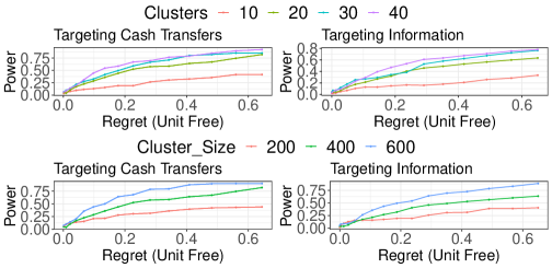
Figure D.1: One-wave experiment in Section 7. $200$ replications. Power plot for $\rho=2$. The panels at the top fix $n=400$ and varies $K$. The panels at the bottom fix $K=20$ and vary $n$.

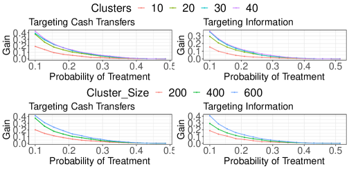
Figure D.2: One-wave experiment. $\rho=2$. Expected percentage increase in welfare from increasing the probability of treatment $\beta$ by $5\%$ upon rejection of $H_{0}$. Here, the x-axis reports $\beta\in[0.1,\cdots,\beta^{*}-0.05]$. The panels at the top fix $n=400$ and vary the number of clusters. The panels at the bottom fix $K=20$ and vary $n$.

Appendix E Additional Algorithms

Algorithm E.1 Welfare maximization with a “non-adaptive” experiment

1:$K$ clusters, $T=p$ periods of experimentation, $n^{-1/2}<\eta_{n}\leq n^{-1/4}$.

2:Create pairs of clusters $\{k,k+1\},k\in\{1,3,\cdots,K-1\}$;

3:$t=0$: For $n$ units in each cluster observe the baseline outcome $Y_{i,0}^{(h)},h\in\{1,\cdots,K\}$. Assign each pair $(k,k+1)$ to an element $\beta^{k}\in\mathcal{G}$, where $\mathcal{G}$ is an equally spaced grid.

4:while $1\leq t\leq T$ do

5:a: Assign treatments as $D_{i,t}^{(h)}\sim\pi(1,\beta^{h}),\quad\beta^{h}=\check{\beta}^{h}\pm\eta_{n}\underline{e}_{t}(h\text{ is even/odd}),$

6:b: For $n$ units in each cluster $h\in\{1,\cdots,K\}$ observe $Y_{i,t}^{(h)}$; estimate for pair $(k,k+1)$, entry $t$, $\widehat{M}_{(k,k+1)}^{(t)}(\beta^{k})=\frac{1}{2\eta_{n}}\Big{[}\bar{Y}_{t}^{k}-\bar{Y}_{0}^{k}\Big{]}-\frac{1}{2\eta_{n}}\Big{[}\bar{Y}_{t}^{k+1}-\bar{Y}_{0}^{k+1}\Big{]}.$

7:end while, return $\hat{\beta}^{ow}$ as in Equation (A.3).

Algorithm E.2 Adaptive Experiment with Many Coordinates

1:Starting value $\beta_{0}\in\mathbb{R}$, $K$ clusters, $T+1$ periods of experimentation, constant $\bar{C}$.

2:Create pairs of clusters $\{k,k+1\},k\in\{1,3,\cdots,K-1\}$;

3:$t=0$(baseline): Assign treatments as $D_{i,0}^{(h)}|X_{i}^{(h)}=x\sim\pi(x;\beta_{0})\text{ for all }h\in\{1,\cdots,K\};$ for $n$ units in each cluster observe $Y_{i,0}^{(h)},h\in\{1,\cdots,K\}$; for cluster $k$ initalize a gradient estimate $\widehat{M}_{k,t}=0$ and initial parameters $\check{\beta}_{k}^{o}=\beta_{0}$.

4:while $1\leq w\leq\check{T}=\frac{T}{p}$ do

5:     for each $j\in\{1,\cdots,p\}$ do ($P_{\mathcal{B}_{1},\mathcal{B}_{2}-\eta_{n}}$ is the projection operator onto $[\mathcal{B}_{1},\mathcal{B}_{2}-\eta_{n}]^{p}$)

$$\check{\beta}_{h}^{w}= P_{\mathcal{B}_{1},\mathcal{B}_{2}-\eta_{n}}\Big{[}\check{\beta}_{h}^{w-1}+\alpha_{\lfloor h+2\rceil,w-1}\widehat{M}_{\lfloor h+2\rceil,w-1}\Big{]},\quad\lfloor h\rceil=h1\{h\leq K\}+(K-h)1\{h>K\}.$$

6:a: Assign treatments as (for a finite constant $\bar{C}$, $\underline{e}_{j}$ in Equation (9))

$$D_{i,t}^{(h)}|X_{i,t}^{(h)}=x\sim\pi(x,\beta_{h,w}),\quad\beta_{h,w}=\check{\beta}_{h}^{w}\pm\eta_{n}\underline{e}_{j}(h\text{ is even/odd}),\quad\bar{C}n^{-1/2}<\eta_{n}<\bar{C}n^{-1/4}$$

7:b: For $n$ units in clusters $h\in\{1,\cdots,K\}$ observe $Y_{i,t}^{(h)}$, and for pair $\{k,k+1\}$, estimate $\widehat{M}_{k,w}^{(j)}=\widehat{M}_{k+1,w}^{(j)}=\frac{1}{2\eta_{n}}\Big{[}\bar{Y}_{t}^{(k)}-\bar{Y}_{0}^{(k)}\Big{]}-\frac{1}{2\eta_{n}}\Big{[}\bar{Y}_{t}^{(k+1)}-\bar{Y}_{0}^{(k+1)}\Big{]}.$

8:c: $t\leftarrow t+1$.

9:     end for

10:d: $w\leftarrow w+1$.

11:end while , return $\hat{\beta}^{*}=\frac{1}{K}\sum_{k=1}^{K}\check{\beta}_{k}^{\check{T}}$

Algorithm E.3 Dynamic Treatment Effects with $\beta\in\mathbb{R}$

1:Parameter space $\mathcal{B}$, clusters $\{1,\cdots,K\}$, two periods $\{t,t+1\}$, perturbation $\eta_{n}$.

2:Group clusters into triads $r\in\{1,\cdots,K/3\}$ with consecutive indeces $\{k,k+1,k+2\}$; construct a grid of parameters $\mathcal{G}\subset[0,1]^{2}$ equally spaced on $[0,1]^{2}$; assign each parameter $(\beta_{1}^{r},\beta_{2}^{r})\in\mathcal{G}$ to a different triad $r$.

3:For each $r\in\{1,\cdots,K/3\}$, and triad $(k,k+1,k+2)$ randomize treatments

$$\small\begin{aligned} D_{i,t}^{(k)}|X_{i}^{(k)},\beta_{1}^{r},\beta_{2}^{r}&\sim\pi(X_{i}^{(k)},\beta_{2}^{r}),\quad&D_{i,t+1}^{(k)}|X_{i}^{(k)},\beta_{1}^{r},\beta_{2}^{r}\sim\pi(X_{i}^{(k)},\beta_{1}^{r}),\\ D_{i,t}^{(k+1)}|X_{i}^{(k)},\beta_{1}^{r},\beta_{2}^{r}&\sim\pi(X_{i}^{(k)},\beta_{2}^{r}+\eta_{n}),\quad&D_{i,t+1}^{(k+1)}|X_{i}^{(k)},\beta_{1}^{r},\beta_{2}^{r}\sim\pi(X_{i}^{(k)},\beta_{1}^{r})\\ D_{i,t}^{(k+2)}|X_{i}^{(k)},\beta_{1}^{r},\beta_{2}^{r}&\sim\pi(X_{i}^{(k)},\beta_{2}^{r}),\quad&D_{i,t+1}^{(k+2)}|X_{i}^{(k)},\beta_{1}^{r},\beta_{2}^{r}\sim\pi(X_{i}^{(k)},\beta_{1}^{r}+\eta_{n})\end{aligned}.$$ (E.1)

4:For each $k\in\{1,4,\cdots,K-2\}$ estimate

$$\widehat{g_{1,k}}=\frac{\bar{Y}_{t+1}^{(k)}-\bar{Y}_{t+1}^{(k+2)}}{\eta_{n}},\quad\widehat{g_{2,k}}=\frac{\bar{Y}_{t+1}^{(k)}-\bar{Y}_{t+1}^{(k+1)}}{\eta_{n}},\quad\widetilde{\Gamma}_{k}=\frac{1}{3}\sum_{h\in\{k,k+1,k+2\}}\bar{Y}_{t+1}^{(h)}$$ (E.2)

Appendix F Additional Extensions

F.1 Staggered adoption

In this section, we sketch the experimental design in the presence of staggered adoption, i.e., when treatments are assigned only once to individuals and post-treatment outcomes are collected once. The algorithm works similarly to what was discussed in Section 4 with one small difference: every period, we only collect information from a given clusters’ pair and update the policy for the subsequent pair and proceed in an iterative fashion.

Theorem F.1 (In-sample regret).

Let the conditions in Theorem 4.3 hold and let $\beta\in\mathbb{R}$, with $\check{\beta}^{t}$ estimated as in Algorithm F.1. Then $P\Big{(}\frac{1}{T}\sum_{t=1}^{T}\Big{[}W(\beta^{*})-W(\check{\beta}^{t})\Big{]}\leq\bar{C}\frac{p\log(T)}{T}\Big{)}\geq 1-1/n$ for a finite constant $\bar{C}<\infty$.

See Appendix G.2 for the proof. The disadvantage of the staggered adoption case is that we cannot control the in-sample regret worst-case over all clusters as in Section 4, but only the average regret across clusters.

Algorithm F.1 Adaptive Experiment with staggered adoption

1:Starting value $\beta\in\mathbb{R}$, $K$ clusters, $T+1$ periods of experimentation.

2:Create pairs of clusters $\{k,k+1\},k\in\{1,3,\cdots,K-1\}$;

3:$t=0$:

4:a: For $n$ units in each cluster observe the baseline outcome $Y_{i,0}^{(h)},h\in\{1,\cdots,K\},\check{\beta}^{0}=\beta$.

5:b: Initalize a gradient estimate $\widehat{M}_{t}=0$

6:while $1\leq t\leq T$ do

7:a: Sample without replaceent one pair of clusters $\{k,k+1\}$ not observed in previous iterations;

8:b: Define $\check{\beta}^{t}=\check{\beta}^{t-1}+\alpha_{t}\widehat{M}_{t};$

9:c: Assign treatments as

$$D_{i,t}^{(h)}\sim\pi(1,\beta_{t}),\quad\beta_{t}=\begin{cases}&\check{\beta}^{t}+\eta_{n}\text{ if }h\text{ is even}\\ &\check{\beta}^{t}-\eta_{n}\text{ if }h\text{ is odd}\end{cases},\quad n^{-1/2}<\eta_{n}\leq n^{-1/4}$$

10:d: For $n$ units in each cluster $h\in\{1,\cdots,K\}$ observe $Y_{i,t}^{(h)}$.

11:end while

12:     Return $\hat{\beta}^{*}=\check{\beta}^{T}$

F.2 Extensions for the network formation model

Consider the following equation:

$$(X_{i}^{(k)},U_{i}^{(k)})\sim_{i.i.d.}F_{U|X}F_{X},\quad A_{i,j}^{(k)}=l\Big{(}X_{i}^{(k)},X_{j}^{(k)},U_{i}^{(k)},U_{j}^{(k)},\omega_{i,j}^{(k)}\Big{)}1\{i_{k}\leftrightarrow j_{k}\}$$ (F.1)

where $\omega_{i,j}^{(k)}\Big{|}\Big{\{}\omega_{u,v}^{(k)}\Big{\}}_{(u,v)\neq(i,j),(u,v)\neq(j,i)},X^{(k)},U^{(k)},\nu^{(k)}\sim_{i.i.d.}F_{\omega}.$

Intuitively, Equation (F.1) states that the connections form also based on unobservables $\omega_{i,j}$ which are drawn independently for each pair $(i,j)$ (note we can have $\omega_{i,j}=\omega_{j,i}$). We can now state the following lemma.

Lemma F.2 (Outcomes).

Under Assumption 2.1, with a network formation as in Equation (F.1), Assumption 2.2, under an assignment in Assumption 2.3 with exogenous (i.e., not data-dependent) $\beta_{k,t}$, Lemma B.4 (and so Lemma 2.1) hold.

The proof is in Appendix G.3. Lemma F.2 implies that our results (and derivations) for inference and estimation directly extend with network formation as in Equation (F.1). One exception is the theorem in Section 5 which instead holds under some minor modification to the proof, which we omit for brevity.

Finally, it is also possible to extend Lemma 2.1 to settings where the network also depends on others’ unobservables. Specifically, consider the following extension:

$$(X_{i}^{(k)},U_{i}^{(k)})\sim_{i.i.d.}F_{U|X}F_{X},\quad A_{i,j}^{(k)}=l\Big{(}X_{i}^{(k)},X_{j}^{(k)},U_{i}^{(k)},U_{j}^{(k)},U_{v:1\{i_{k}\sim v_{k}\}=1},U_{v^{\prime}:1\{j_{k}\sim v_{k}^{\prime}\}=1}\Big{)}1\{i_{k}\leftrightarrow j_{k}\}.$$ (F.2)

Equation (F.2) states that the connection between individual $i$ and $j$ can depend not only on unobservables of $i$ and $j$, but also unobservables of all the possible connections of both individual $i$ and individual $j$. Following a similar argument of Lemma B.4, we can show

$$Y_{i,t}^{(k)}=y\Big{(}X_{i}^{(k)},\beta_{k,t}\Big{)}+\varepsilon_{i,t}^{(k)}+\alpha_{t}+\tau_{k},\quad\mathbb{E}_{\beta_{k,t}}\Big{[}\varepsilon_{i,t}^{(k)}|X_{i}^{(k)}\Big{]}=0,$$ (F.3)

for some function $y(\cdot)$ unknown to the researcher. Therefore, our results for estimation and inference hold also in this setting.

F.3 Selection of $\eta_{n}$: rule of thumb

In this subsection we provide a rule of thumb for selecting $\eta_{n}$. Following Theorem 3.1 and following Lemma B.3 which provides exact constants, with probability at least $1-1/n$

$$\Big{|}\widehat{M}_{(k,k+1)}-M(\beta)\Big{|}\leq\sqrt{\frac{2\sigma^{2}\gamma_{N}\log(2\gamma_{N}n)}{n\eta_{n}^{2}}}+c\eta_{n},\quad c=\Big{|}\Big{|}\frac{\partial^{2}m(d,x,\beta)}{\partial\beta^{2}}\Big{|}\Big{|}_{\infty},$$

where the $l_{\infty}$ is taken with respect to each element of the Hessian, $x,\beta$. we cannot directly minimize the upper bound since otherwise we would violate the condition that $\eta_{n}=o(n^{-1/4})$. Instead, we minimize $\min_{\eta_{n}}\sqrt{\frac{2\sigma^{2}\gamma_{N}\log(2\gamma_{N}n)}{n\eta_{n}^{2}}}+c\eta_{n}/s_{n}^{2},s_{n}=o(1),$ where $s_{n}$ penalizes the bias by an $o(1)$ component and chosen below. It follows that for given penalization $s_{n}$ the minimizer of the expression is $\eta_{n}^{2}=\sqrt{\frac{2s_{n}\sigma^{2}\gamma_{N}\log(2\gamma_{N}n)}{nc}}.$ Let $s_{n}=\gamma_{N}/(n^{1/4}\log(n\gamma_{N}))$, assumed to be $o(1)$ for inference by assumption. we can then write the solution to the optimization problem as $\gamma_{N}\sqrt{\frac{2\sigma^{2}}{c}}n^{-5/16}\approx\gamma_{N}\sqrt{\frac{2\sigma^{2}}{c}}n^{-1/3}.$ Here, we can replace $\sigma^{2}$ and $c$ with some out-of-sample estimates of the outcomes’ variance and curvature. Whenever the researcher does not have a good guess for $\gamma_{N}$, we recommend choosing $\eta_{n}=\sqrt{\frac{2\sigma^{2}}{c}}n^{-1/3}$ (without the term $\gamma_{N}$) which also leads to valid inference, but slightly smaller small-sample bias (and larger small-sample variance) than the optimal choice. Finally, since researcher may impose small sample upper bound on the bias, the suggested rule of thumb is

$$\eta_{n}=\begin{cases}&\sqrt{\frac{2\sigma^{2}}{c}}n^{-1/3}\quad\text{ if }\sqrt{\frac{2\sigma^{2}}{c}}n^{-1/3}\leq H\\ &H\text{ otherwise}\end{cases}$$

where $Hc$ denotes an upper bound on the bias of the estimator imposed by the researcher.

Appendix G Additional proofs for the extensions

G.1 Proof of Theorem A.8

In this subsection, we derive the theorem for the gradient descent method under Assumption A.5. The derivation is split into the following lemmas.

Definition G.1 (Oracle gradient descent).

We define for positive constants $\infty>\mu,\kappa>0$, $\kappa$ as defined in Lemma G.1, arbitrary $v\in(0,1)$, $\alpha_{w}=\frac{J}{\check{T}^{1/2-v/2}||M(\beta_{w-1}^{*})||},J<1$

$$\beta_{w}^{*}=\begin{cases}&P_{\mathcal{B}_{1},\mathcal{B}_{2}}\Big{[}\beta_{w-1}^{*}+\alpha_{w-1}M(\beta_{w-1}^{*})\Big{]}\text{ if }||M(\beta_{w}^{*})||_{2}\geq\frac{\kappa}{\mu\check{T}^{1/2-v/2}}\\ &\beta^{*}_{w-1}\text{ otherwise}\end{cases}\quad\beta_{1}^{*}=\beta_{0},$$ (G.1)

Lemma G.1 (Adaptive gradient descent for quasi-concave functions and locally strong concave).

Let $\mathcal{B}$ be compact. Define $G=\max\{\sup_{\beta\in\mathcal{B}}2||\beta||^{2},1\}$. Let Assumption 3.1, 4.1, A.5 hold. Let $\kappa$ be a positive finite constant, defined as in Equation (G.2). Then for any $v\in(0,1)$, for $\check{T}\geq((G+1)/J)^{1/v}$, the following holds: $||\beta_{\check{T}}^{*}-\beta^{*}||^{2}\leq\kappa\check{T}^{-1+v}.$

Proof of Lemma G.1.

To prove the statement, we use properties of gradient descent methods with gradient norm rescaling (Hazan et al., 2015), with modifications to the original arguments to explicitely obtain a rate $T^{-1+v}$ for an arbitrary small $v$.

Preliminaries

Clearly, if the algorithm terminates at $w$, under Assumption A.5 (B), this implies that $||\beta_{w}^{*}-\beta^{*}||_{2}^{2}\leq\kappa\check{T}^{-1+v},$ proving the claim. Therefore, assume that the algorithm did not terminate at time $w$. This implies that for any $\check{w}\geq 1$, $||\beta_{\check{w}}^{*}-\beta^{*}||_{2}^{2}>\kappa\check{T}^{-1+v}$. Define $\epsilon=\check{T}^{-1+v}$ and let $\nabla_{w}$ be the gradient evaluated at $\beta_{w}^{*}$. For every $\beta\in\mathcal{B}$, define $H(\beta)\Big{|}_{[\beta^{*},\beta]}$ the Hessian evaluated at some point $\tilde{\beta}\in[\beta^{*},\beta]$, such that

$$W(\beta)=W(\beta^{*})+\frac{1}{2}(\beta-\beta^{*})^{\top}H(\beta)\Big{|}_{[\beta^{*},\beta]}(\beta-\beta^{*}),$$

which always exists by the mean-value theorem and differentiability of the objective function. Define

$$\frac{1}{2}(\beta-\beta^{*})^{\top}H(\beta)\Big{|}_{[\beta^{*},\beta]}(\beta-\beta^{*})=f(\beta)\leq 0,$$

where the inequality follows by definition of $\beta^{*}$ (note that $f(\beta)$ also depends on $\tilde{\beta}$, whose dependence we implicitely suppressed). Finally, note that $-|\lambda_{max}|||\beta-\beta^{*}||^{2}\leq f(\beta)\leq-|\lambda_{\min}|||\beta-\beta^{*}||^{2}$ for constants $\lambda_{\max}>\lambda_{\min}>0$. The lower bound follows directly by Assumption 3.1, while the upper bound follows directly from Assumption A.5 (C).

Cases

Define

$$\kappa=\frac{|\lambda_{max}|}{|\lambda_{min}|}\geq 1.$$ (G.2)

Observe now that if $||\beta_{w}^{*}-\beta^{*}||^{2}\leq\epsilon\kappa$, the claim trivially holds. Therefore, consider the case where $||\beta_{w}^{*}-\beta^{*}||^{2}>\epsilon\kappa.$

Comparisons within the neighborhood

Take $\tilde{\beta}=\beta^{*}-\sqrt{\epsilon}\frac{\nabla_{w}}{||\nabla_{w}||_{2}}$. Observe that

$$W(\tilde{\beta})-W(\beta_{w}^{*}) =\frac{1}{2}(\tilde{\beta}-\beta^{*})^{\top}H(\tilde{\beta})\Big{|}_{[\beta^{*},\tilde{\beta}]}(\tilde{\beta}-\beta^{*})-\frac{1}{2}(\beta^{*}_{w}-\beta^{*})^{\top}H(\beta_{w}^{*})\Big{|}_{[\beta^{*},\beta_{w}^{*}]}(\beta_{w}^{*}-\beta^{*})$$

$$\geq-|\lambda_{\max}|\epsilon+|\lambda_{\min}|\epsilon\kappa=0.$$

As a result, for all $\beta_{w}^{*}:||\beta_{w}^{*}-\beta^{*}||^{2}>\epsilon\kappa$, using quasi-concavity

$$\nabla_{w}^{\top}(\tilde{\beta}-\beta^{*}_{w})\geq 0\Rightarrow\nabla_{w}^{\top}(\beta^{*}-\beta_{w}^{*})\geq\sqrt{\epsilon}||\nabla_{w}||_{2}$$ (G.3)

Plugging in the above expression in the definition of $\beta_{w}^{*}$

By construction of the algorithm, we write

$$||\beta^{*}-\beta_{w+1}^{*}||^{2}\leq||\beta^{*}-\beta_{w}^{*}||^{2}-2\alpha_{w}J\nabla_{w}^{\top}(\beta^{*}-\beta_{w}^{*})+J^{2}\alpha_{w}^{2}||\nabla_{w}||^{2}.$$

By Equation (G.3), we can write $||\beta^{*}-\beta_{w+1}^{*}||^{2}\leq||\beta^{*}-\beta_{w}^{*}||^{2}-2J\alpha_{w}\sqrt{\epsilon}||\nabla_{w}||_{2}+J^{2}\alpha_{w}^{2}||\nabla_{w}||^{2}.$ Plugging in the expression for $\alpha_{w}$, and using the fact that $J\leq 1$, we have $||\beta^{*}-\beta_{w+1}^{*}||^{2}\leq||\beta^{*}-\beta_{w}^{*}||^{2}-J\epsilon.$

Recursive argument

Recall that since the algorithm did not terminate, $||\beta^{*}-\beta_{\check{w}}^{*}||^{2}>\epsilon\kappa$, for all $\check{w}\leq w$. Using this argument recursively, we obtain

$$||\beta^{*}-\beta_{\check{T}}^{*}||^{2}\leq||\beta^{*}-\beta_{0}||^{2}-J\sum_{s=1}^{\check{T}}\epsilon=2\max_{\beta\in\mathcal{B}}||\beta||^{2}-J\check{T}^{v}\leq G+1-J\check{T}^{v}.$$

Whenever $\check{T}>(G/J+1/J)^{1/v}$, we have a contradiction. The proof completes. ∎

Lemma G.2.

Let Assumption 2.1, 2.2, 4.1, A.5 hold. Assume that

$$\epsilon_{n}\geq\sqrt{p}\Big{[}\bar{C}\sqrt{\gamma_{N}\frac{\log(\gamma_{N}\check{T}K/\delta)}{\eta_{n}^{2}n}}+\eta_{n}\Big{]},\quad\frac{1}{4\mu\check{T}^{1/2-v/2}}-\epsilon_{n}\geq 0$$

for a finite constant $\bar{C}<0$.

Then, with probability at least $1-\delta$, for any $\delta\in(0,1)$ for any $w\leq\check{T}$,

$$\text{ either }(i)\Big{|}\Big{|}\check{\beta}_{k}^{w}-\beta_{w}^{*}\Big{|}\Big{|}_{\infty}=\mathcal{O}(P_{w}(\delta)+p\eta_{n}),\text{ or }(ii)\Big{|}\Big{|}\check{\beta}_{k}^{w}-\beta^{*}\Big{|}\Big{|}_{2}^{2}\leq\frac{p}{\check{T}^{1-v}}$$

where $P_{1}(\delta)=\mathrm{err}(\delta)$ and $P_{w}(\delta)=\frac{2\sqrt{p}}{\nu_{n}}Bp\frac{1}{\check{T}^{1/2-v/2}}P_{w-1}(\delta)+P_{w-1}(\delta)+\frac{2\sqrt{p}}{\nu_{n}}\frac{1}{\check{T}^{1/2-v/2}}\mathrm{err}(\delta)$, for a finite constant $B<\infty$, and $\mathrm{err}(\delta)\leq c_{0}\Big{(}\sqrt{\gamma_{N}\frac{\log(\gamma_{N}p\check{T}K/\delta)}{\eta_{n}^{2}n}}+p\eta_{n}\Big{)}$, with $\nu_{n}=\frac{1}{\mu\check{T}^{1/2-v/2}}-2\epsilon_{n}$, and a finite constant $c_{0}<\infty$.

Proof of Lemma G.2.

First, by Lemma 4.1, the estimated coefficients are exogenous. Hence, by invoking Lemma B.7 and the union bound, we can write for every $k$ and $t$, $\delta\in(0,1)$, $|\check{M}_{k,w}^{(j)}-M^{(j)}(\check{\beta}_{k+2}^{w})|\leq c_{0}\Big{(}\sqrt{\gamma_{N}\frac{\log(\gamma_{N}K\check{T}/\delta)}{\eta_{n}^{2}n}}+\eta_{n}\Big{)}.$ We now proceed by induction. We first prove the statement, assuming that the constraint is always attained. We then discuss the case of the constrained solution. Define $B=\sup_{\beta}\Big{|}\Big{|}\frac{\partial^{2}W(\beta)}{\partial\beta^{2}}\Big{|}\Big{|}_{\infty}.$

Unconstrained case

Consider $w=1$. Then since all clusters start from the same starting point $\beta_{0}$ recall that $(\beta_{1}^{*}=\beta_{0})$, we can write with probability $1-\delta$, by the union bound over $p$ (which hence enters in the $\log(p)$ component of $\mathrm{err}_{n}$) and Lemma B.7 $\Big{|}\Big{|}\check{M}_{k,1}-M(\beta_{1}^{*})\Big{|}\Big{|}_{\infty}\leq\mathrm{err}(\delta).$ Consider now the case where the algorithm stops. This implies that it must be that $||\check{M}_{k,1}||_{2}\leq\frac{1}{\mu\check{T}^{1/2-v/2}}-\epsilon_{n}$. By Lemma B.7

$$||M(\beta_{1}^{*})||_{2}\leq||\check{M}_{k,1}||_{2}+\sqrt{p}\mathrm{err}(\delta)\leq\frac{1}{\mu\check{T}^{1/2-v/2}}-\epsilon_{n}+\sqrt{p}\mathrm{err}(\delta)\leq\frac{1}{\mu\check{T}^{1/2-v/2}}.$$ (G.4)

since $\epsilon_{n}\geq\sqrt{p}\mathrm{err}(\delta)$. As a result, also the oracle algorithm stops at $\beta_{1}^{*}$ by construction of $\epsilon_{n}$. Suppose the algorithm does not stop. Then it must be that $||\check{M}_{k,1}||\geq\frac{1}{\mu\check{T}^{1/2-v/2}}-\epsilon_{n}$ and

$$||V_{1}(\beta_{1}^{*})||\geq\frac{1}{\mu\check{T}^{1/2-v/2}}-\epsilon_{n}-\sqrt{p}\mathrm{err}_{1}\geq\frac{1}{\mu\check{T}^{1/2-v/2}}-2\epsilon_{n}:=\nu_{n}>0.$$

Observe now that

$$\Big{|}\Big{|}\frac{\check{M}_{k,1}}{||\check{M}_{k,1}||_{2}}-\frac{M(\beta_{1}^{*})}{||M(\beta_{1}^{*})||_{2}}\Big{|}\Big{|}_{\infty} \leq\Big{|}\Big{|}\frac{\check{M}_{k,1}-M(\beta_{1}^{*})}{||M(\beta_{1}^{*})||_{2}}\Big{|}\Big{|}_{\infty}+\Big{|}\Big{|}\frac{\check{M}_{k,1}(||\check{M}_{k,1}||_{2}-||M(\beta_{1}^{*})||_{2})}{||M(\beta_{1}^{*})||_{2}||\check{M}_{k,1}||_{2}}\Big{|}\Big{|}_{\infty}$$ (G.5)

$$\leq\Big{|}\Big{|}\frac{\check{M}_{k,1}-M(\beta_{1}^{*})}{||M(\beta_{1}^{*})||_{2}}\Big{|}\Big{|}_{\infty}+\sqrt{p}\Big{|}\Big{|}\frac{\check{M}_{k,1}-M(\beta_{1}^{*})}{||M(\beta_{1}^{*})||_{2}}\Big{|}\Big{|}_{\infty}.$$

The last inequality follows from the reverse triangular inequalities and standard properties of the norms. Then with probability at least $1-\delta$, for any $\delta\in(0,1)$ $\eqref{eqn:p}\leq\frac{1}{\nu_{n}}\times 2\sqrt{p}\mathrm{err}(\delta).$ completing the claim for $w=1$. Consider now a general $w$. Define the error until time $w-1$ as $P_{w-1}$.Then for every $j\in\{1,\cdots,p\}$, by Assumption 3.1, we have with probability at least $1-w\delta$ (using the union bound), and letting $\mathbf{1}_{p}=[1,\cdots,1]\in\mathbb{R}^{p}$,

$$\check{M}_{k,w}^{(j)}=M^{(j)}(\check{\beta}_{k+2}^{w})+\mathrm{err}(\delta)=M^{(j)}(\beta_{w}^{*}+\mathbf{1}_{p}P_{w}(\delta))+\mathrm{err}(\delta)$$

$$\Rightarrow\Big{|}\Big{|}\check{M}_{k,w}-M(\beta_{w}^{*})\Big{|}\Big{|}_{\infty}\leq BpP_{w}(\delta)+\mathrm{err}(\delta),$$

where the above inequality follows by the mean-value theorem and Assumption 3.1. Suppose now that $||\check{M}_{k,w}||_{2}\leq\frac{1}{\mu\check{T}^{1/2-v/2}}-\epsilon_{n}$. Then for the same argument as in Equation (G.4), we have $||M(\check{\beta}_{k}^{w})||_{2}\leq\frac{1}{\mu\check{T}^{1/2-v/2}}.$ Under Assumption A.5 (B) this implies that $||\check{\beta}_{k}^{w}-\beta^{*}||_{2}^{2}\leq\frac{1}{\check{T}^{1-v}},$ which proves the statement. Suppose instead that the algorithm does not stop. Then we can write by the induction argument

$$\Big{|}\Big{|}\check{\beta}_{k}^{w}+\frac{1}{\check{T}^{1/2-v/2}}\frac{\check{M}_{k,w}}{||\check{M}_{k,w}||_{2}}-\beta_{w}^{*}-\frac{1}{\check{T}^{1/2-v/2}}\frac{M(\beta_{w}^{*})}{||M(\beta_{w}^{*})||_{2}}\Big{|}\Big{|}_{\infty}\leq P_{w}(\delta)+\frac{1}{\check{T}^{1/2-v/2}}\underbrace{\Big{|}\Big{|}\frac{\check{M}_{k,w}}{||\check{M}_{k,w}||_{2}}-\frac{M(\beta_{w}^{*})}{||M(\beta_{w}^{*})||_{2}}\Big{|}\Big{|}_{\infty}}_{(B)}.$$ (G.6)

Using the same argument in Equation (G.5), we have with probability at least $1-\delta$, $(B)\leq\frac{2\sqrt{p}}{\nu_{n}}\Big{[}\mathrm{err}(\delta)+BpP_{w}(\delta)\Big{]},$ which completes the proof for the unconstrained case. The $\check{T}$ component in the error expression follows from the union bound across all $\check{T}$ events.

Constrained case

Since the statement is true for $w=1$, we can assume that it is true for all $s\leq w-1$ and prove the statement by induction. Since $\mathcal{B}$ is a compact space, we can write

$$\Big{|}\Big{|}P_{\mathcal{B}_{1},\mathcal{B}_{2}-\eta_{n}}\Big{[}\sum_{s=1}^{w}\alpha_{k,s}\check{M}_{k,s}\Big{]}-P_{\mathcal{B}_{1},\mathcal{B}_{2}}\Big{[}\sum_{s=1}^{w}\alpha_{s}M(\beta_{s}^{*})\Big{]}\Big{|}\Big{|}_{\infty}$$

$$\leq\Big{|}\Big{|}P_{\mathcal{B}_{1},\mathcal{B}_{2}-\eta_{n}}\Big{[}\sum_{s=1}^{w}\alpha_{k,s}\check{M}_{k,s}\Big{]}-P_{\mathcal{B}_{1},\mathcal{B}_{2}-\eta_{n}}\Big{[}\sum_{s=1}^{w}\alpha_{s}M(\beta_{s}^{*})\Big{]}\Big{|}\Big{|}_{\infty}+p\mathcal{O}(\eta_{n})$$

$$\leq 2\Big{|}\Big{|}\sum_{s=1}^{w}\alpha_{k,s}\check{M}_{k,s}-\sum_{s=1}^{w}\alpha_{s}M(\beta_{s}^{*})\Big{|}\Big{|}_{\infty}+p\mathcal{O}(\eta_{n}).$$

For the first component in the last inequality, we follow the same argument as above. ∎

Lemma G.3.

Let the conditions in Lemma G.2 hold. Then with probability at least $1-\delta$, for any $k\in\{1,\cdots,K\}$, for any $v\in(0,1),\delta\in(0,1)$, $\check{T}\geq\zeta^{1/v}$,

$$||\beta^{*}-\check{\beta}_{k}^{\check{T}}||_{2}^{2}\leq\frac{\kappa}{\check{T}^{1-v}}+\check{T}e^{Bp\sqrt{p}\check{T}}\times c_{0}\Big{(}\gamma_{N}\frac{\log(p\gamma_{N}\check{T}K/\delta)}{\eta_{n}^{2}n}+p^{2}\eta_{n}^{2}\Big{)},$$

with $0<\zeta,\kappa,B<\infty$ being constants independent on $(n,\check{T})$ and $\epsilon_{n}$ as defined in Lemma G.2, and a finite constant $c_{)}<\infty$.

Proof.

We invoke Lemma G.2. Observe that we only have to check that the result holds for (i) in Lemma G.2, since otherwise the claim trivially holds. Using the triangular inequality, we can write $||\beta^{*}-\check{\beta}_{k}^{\check{T}}||_{2}^{2}\leq||\beta^{*}-\beta_{\check{T}}^{*}||_{2}^{2}+||\check{\beta}_{k}^{\check{T}}-\beta_{\check{T}}^{*}||_{2}^{2}.$ The first component on the right-hand side is bounded by Lemma G.1, with $\check{T}\geq\zeta^{1/v},\zeta$ being a constant defined in Lemma G.1.

Using Lemma G.2, we bound with probability at least $1-\delta$, the second component as follows $||\check{\beta}_{k}^{\check{T}}-\beta_{\check{T}}^{*}||_{2}^{2}\leq p||\check{\beta}_{k}^{\check{T}}-\beta_{\check{T}}^{*}||_{\infty}^{2}=p\times\mathcal{O}(P_{\check{T}}^{2}(\delta)).$ We conclude the proof by explicitly defining recursively, for all $1<w\leq\check{T}$,

$$P_{w}=(1+\frac{2Bp\sqrt{p}}{\nu_{n}\check{T}^{1/2-v/2}})P_{w-1}+\frac{1}{\check{T}^{1/2-v/2}}\tilde{\mathrm{err}}_{n}(\delta),\quad P_{1}=\tilde{\mathrm{err}}_{n}(\delta).$$

where $\tilde{\mathrm{err}}_{n}(\delta)=\frac{2\sqrt{p}}{\nu_{n}}c_{0}(\sqrt{\gamma_{N}\frac{\log(pTK/\delta)}{\eta_{n}^{2}n}}+p\eta_{n})$, and $B<\infty$ denotes a finite constant. Using a recursive argument, we obtain $P_{w}=\tilde{\mathrm{err}}_{n}(\delta)\sum_{s=1}^{w}\alpha_{s}\prod_{j=s}^{w}(\frac{2Bp\sqrt{p}}{\nu_{n}\check{T}^{1/2-v/2}}+1).$ Recall now that $\nu_{n}\geq\frac{1}{2\mu\check{T}^{1/2-v/2}}$, for $\varepsilon_{n}$ as in Lemma G.2. As a result we can bound the above expression as

$$\sum_{s=1}^{w}\alpha_{s}\prod_{j=s}^{w}(\frac{2Bp\sqrt{p}}{\nu_{n}\check{T}^{1/2-v/2}}+1)\leq\sum_{s=1}^{w}\alpha_{s}\prod_{j=s}^{w}(\frac{4\mu\check{T}^{1/2-v/2}Bp\sqrt{p}}{\check{T}^{1/2-v/2}}+1)\leq\sum_{s=1}^{w}\alpha_{s}\exp\Big{(}\sum_{j=s}^{w}4\mu Bp\sqrt{p}\Big{)}.$$

Now we have $\exp\Big{(}\sum_{j=s}^{w}4\mu Bp\sqrt{p}\Big{)}\leq\exp\Big{(}4\mu\check{T}Bp\sqrt{p}\Big{)},$ since $w\leq\check{T}$. We now write

$$P_{w}(\delta)\leq\tilde{\mathrm{err}}_{n}(\delta)\sum_{s=1}^{w}\alpha_{s}\exp\Big{(}4\mu\check{T}Bp\sqrt{p}\Big{)}\leq\tilde{\mathrm{err}}_{n}(\delta)\check{T}^{1/2+v}\exp\Big{(}8\mu^{2}\check{T}Bp\sqrt{p}\Big{)}.$$

∎

Corollary 7.

Theorem A.8 holds.

Proof.

Consider Lemma G.2 where we choose $\delta=1/n$. Observe that we choose $\epsilon_{n}\leq\frac{1}{4\mu\check{T}^{1/2-v/2}}$, which is attained by the conditions in Lemma G.2 as long as $n$ is small enough such that

$$\sqrt{p}\Big{[}\bar{C}\sqrt{\log(n)\gamma_{N}\frac{\log(p\gamma_{N}\check{T}K)}{\eta_{n}^{2}n}}+\eta_{n}\Big{]}\leq\frac{1}{4\mu\check{T}^{1/2-v/2}}$$

attained under the assumptions stated in Lemma G.2. As a result, we have $\nu_{n}=\frac{1}{4\mu\check{T}^{1/2-v/2}}$. By Lemma G.3 for all $k$, with probability at least $1-1/n$, $||\check{\beta}_{k}^{\check{T}}-\beta^{*}||^{2}\lesssim\frac{p}{\check{T}^{1-v}}.$ Also, we have $||\beta^{*}-\frac{1}{K}\sum_{k}\check{\beta}_{k}^{\check{T}}||_{2}^{2}\leq\frac{1}{K}\sum_{k}||\check{\beta}_{k}^{\check{T}}-\beta^{*}||^{2}.$ The proof concludes by Theorem G.3 and Assumption 3.1, after observing that $W(\beta^{*})-W(\hat{\beta}^{*})\lesssim||\beta^{*}-\hat{\beta}^{*}||_{2}^{2}.$ ∎

G.2 Proof of Theorem F.1

The proof mimics the proof of Theorem 4.3.

Consider Lemma B.10 where we choose $\delta=1/n$. Note that we can directly apply Lemma B.10 also to the gradient estimated with Algorithm F.1, since, by the circular-cross fitting argument, each parameter $\check{\beta}_{k}^{w}$ is estimated using sequentially pairs of different clusters as in Algorithm F.1. The rest of the proof follows verbatim from the one of Theorem 4.3.

G.3 Proof of Lemma F.2

The proof follows similarly to the proof of Lemma B.4, here taking into account also the component $\omega_{i,j}$. Under Assumption 2.2, we can write for some function $g$,

$$r\Big{(}D_{i,t}^{(k)},D_{j:A_{i,j}^{(k)}>0,t}^{(k)},X_{i}^{(k)},X_{j:A_{i,j}^{(k)}>0}^{(k)},A_{i}^{(k)},U_{i}^{(k)},U_{j:A_{i,j}^{(k)}>0}^{(k)},\nu_{i,t}^{(k)}\Big{)}=g(Z_{i,t}^{(k)}).$$

Here, $Z_{i,t}^{(k)}$ depends on $A_{i}^{(k)}$, i.e., the edges of individual $i$, and on unobservables and observables of all those individuals such that $A_{i,j}^{(k)}>0$, namely,

$$Z_{i,t}^{(k)}=\Big{[}D_{i,t}^{(k)},X_{i}^{(k)},U_{i}^{(k)},\nu_{i,t}^{(k)},A_{i}^{(k)}\otimes\Big{(}X^{(k)},U^{(k)},D_{t}^{(k)}\Big{)},\Big{\{}\Big{[}X_{j}^{(k)},U_{j}^{(k)},\omega_{i,j}^{(k)}\Big{]},j:1\{i_{k}\leftrightarrow j_{k}\}=1\Big{\}}\Big{]}.$$

Importantly, under Equation (F.1), $A_{i}^{(k)}$ is a function of $\Big{\{}\Big{[}X_{j}^{(k)},U_{j}^{(k)},\omega_{i,j}^{(k)}\Big{]},j:1\{i_{k}\leftrightarrow j_{k}\}=1\Big{\}},$ only, and each entry depends on $(X_{j},U_{j},X_{i},U_{i},\omega_{i,j})$ through the same function $l$ for each individual. What is important, is that $\sum_{j}1\{i_{k}\leftrightarrow j_{k}\}=\gamma_{N}^{1/2}$ for each unit $i$. Therefore, for some function $\tilde{g}$ (which depends on $l$ in Assumption 2.1), we can equivalently write

$$Z_{i,t}^{(k)}=\tilde{g}(D_{i,t}^{(k)},\nu_{i,t}^{(k)},X_{i}^{(k)},U_{i}^{(k)},\tilde{Z}_{i,t}^{(k)}),\quad\tilde{Z}_{i,t}^{(k)}=\Big{\{}\Big{[}X_{j}^{(k)},U_{j}^{(k)},D_{j,t}^{(k)},\omega_{i,j}^{(k)}\Big{]},j:1\{i_{k}\leftrightarrow j_{k}\}=1\Big{\}},$$

where $\tilde{Z}_{i,t}^{(k)}$ is the vector of $\Big{[}X_{j}^{(k)},U_{j}^{(k)},D_{j,t}^{(k)},\omega_{i,j}\Big{]}$ of all individuals $j$ with $1\{i_{k}\leftrightarrow j_{k}\}=1$.

Now, observe that since $(U_{i}^{(k)},X_{i}^{(k)})\sim_{i.i.d.}F_{X|U}F_{U}$, $\omega_{i,j}\sim F_{\omega}$, $\{\nu_{i,t}\}$ are $i.i.d.$ conditionally on $U^{(k)},X^{(k)},\omega^{(k)}$ and treatments are randomized as in Assumption 2.3, we have

$$G_{i,j}^{(k)}=\Big{[}X_{j}^{(k)},U_{j}^{(k)},\nu_{j,t}^{(k)},D_{j,t}^{(k)},\omega_{i,j}^{(k)}\Big{]}\Big{|}\beta_{k,t}\sim\mathcal{D}(\beta_{k,t})$$

are distributed with some distribution $\mathcal{D}(\beta_{k,t})$ which only depends on the exogenous coefficient $\beta_{k,t}$ governing the distribution of $D_{i,t}^{(k)}$ under Definition 2.3. Also, $G_{i,j}^{(k)}$ are independent across $j$ (but not $i$) by the independence assumption of $\omega_{i,j}$. As a result for $\beta_{k,t}$ being exogenous, Lemma 2.1 holds since $\sum_{j}1\{i_{k}\leftrightarrow j_{k}\}=\gamma_{N}^{1/2}$ for all $i$, hence $\tilde{Z}_{i,t}$ are identically (but not independently) distributed across units $i$, since $\tilde{Z}_{i,t}$ is a vector of $\gamma_{N}$ $i.i.d$ random variables, each having the same marginal distribution which does not depend on $i$ (therefore $\tilde{Z}_{i,t}$ has the same joint distribution across $i$).

To show the local dependence result, note that $G_{i,j}^{(k)}$ is mutually independent of $G_{u,v}^{(k)}$ for all $\{(v,u):(v,u)\not\in\{(i,j),(j,i)\},u\neq j\}$ because $\omega_{i,j}$ are independent for different entries $(i,j)$. In addition, $\varepsilon_{i,t}^{(k)}|\beta_{k,t}$ is a measurable function of a vector

$$\Big{[}X_{j}^{(k)},U_{j}^{(k)},\nu_{j,t}^{(k)},D_{j,t}^{(k)},\omega_{i,j}^{(k)}\Big{]}_{j:1\{i_{k}\leftrightarrow j_{k}\}=1}.$$

As a result, under mutual independence of $G_{i,j}$ with $G_{u,v}$ for all $\{(v,u):(v,u)\not\in\{(i,j),(j,i)\},u\neq j\}$, conditional on $\beta_{k,t}$, $\varepsilon_{i,t}^{(k)}$ is mutally independent with $\varepsilon_{v,t}^{(k)}$ for all $v$ such that they are not connected and do not share a common element $\Big{[}X_{j}^{(k)},U_{j}^{(k)},\nu_{j,t}^{(k)},D_{j,t}^{(k)},\omega_{v,j}^{(k)}\Big{]}$, that is, such that $\max_{j}1\{i_{k}\leftrightarrow j_{k}\}1\{v_{k}\leftrightarrow j_{k}\}=0$ (here $1\{v_{k}\leftrightarrow v_{k}\}=1$ for notational convenience). This holds since the edge between $i$ and $v$ is zero almost surely if $1\{v_{k}\leftrightarrow i_{k}\}=0$.

There are at most $\gamma_{N}^{1/2}+\gamma_{N}$ many of $\varepsilon_{v,t}^{(k)}$ which can share a common neighbor with $\varepsilon_{i,t}^{(k)}$ ($\gamma_{N}^{1/2}$ many neighhbors and $\gamma_{N}$ many neighbors of the neighbors), which concludes the proof.

Appendix H Numerical studies: additional results

H.1 One-wave experiment

In Figure H.2 we report the power plot for $\rho=6$. In Figure H.3 we report the welfare gain from increasing $\beta$ by $5\%$ upon rejection of $H_{0}$ for $\rho=6$. In Figure H.6, we report comparisons for different values of $\eta_{n}$.

H.2 Multiple-wave experiment

In Table H.1, we provide comparison with competitors for $\rho=6$. Results are robust as in the main text.

In Figure H.4 we report a comparison among different learning rates, which are the one which rescales by $1/t$, the one that rescales by $1/\sqrt{T}$ and the one that rescales by $1/\sqrt{t}$.

In Figure H.9 we study the adaptive experiment as the starting value is the optimum minus $5\%$ and show that the out-of-sample regret is small and close to zero.

H.3 Calibrated experiment with covariates for cash transfers

In this subsection, we turn to a calibrated experiment where we also control for covariates, as discussed in Section LABEL:sec:overview. we use data from Alatas et al. (2012, 2016). we estimate a function heterogenous in the distance of the household’s village from the district’s center. we use information from approximately four hundred observations, whose eighty percent or more neighbors are observed. We let $X_{i}\in\{0,1\},X_{i}=1$ if the household is far from the district’s center than the median household, and estimate

$$Y_{i}|X_{i}=x\quad=\quad\phi_{0}+\tilde{X}_{i}\tau+D_{i}\phi_{1,x}+\frac{\sum_{j\neq i}A_{j,i}D_{j}}{\max\{\sum_{j\neq i}A_{j,i},1\}}\phi_{2,x}+\Big{(}\frac{\sum_{j\neq i}A_{j,i}D_{j}}{\max\{\sum_{j\neq i}A_{j,i},1\}}\Big{)}^{2}\phi_{3,x}+\eta_{i},$$ (H.1)

where $\eta_{i}$ are unobservables centered on zero conditional on $X_{i}=x$, and $\tilde{X}_{i}$ denotes controls which also include $X_{i}$. Using the estimated parameter, we can then calibrate the simulations as follows.

We let $\eta_{i,t},\sim\mathcal{N}(0,\sigma^{2})$, where $\sigma^{2}$ is the residual variance from the regression. We then generate the network and the covariate as follows:

$$A_{i,j}=1\Big{\{}||U_{i}-U_{j}||_{1}\leq 2\rho/\sqrt{N}\Big{\}},\quad U_{i}\sim_{i.i.d.}\mathcal{N}(0,I_{2}),\quad X_{i}=1\{U_{i}^{(1)}>0\}.$$

Here, $U_{i}^{(1)}$ is continuous and captures a measure of distances. Individuals are more likely to be friends if they have similar distances from the center, and $X_{i}$ is equal to one if an individual is far from the district’s center from the median household. We fix $\rho=1.5$ to guarantee that the objective’s function optimum is approximately equal to the optimum observed from the data (in calibration, the optimum is $\beta\approx 0.26$, while $\beta^{*}\approx 0.29$ on the data). We then generate data

$$Y_{i,t}|X_{i}=x\quad=\quad D_{i}\hat{\phi}_{1,x}+\frac{\sum_{j\neq i}A_{j,i}D_{j}}{\max\{\sum_{j\neq i}A_{j,i},1\}}\hat{\phi}_{2,x}+\Big{(}\frac{\sum_{j\neq i}A_{j,i}D_{j}}{\max\{\sum_{j\neq i}A_{j,i},1\}}\Big{)}^{2}\hat{\phi}_{3,x}+\eta_{i,t}.$$ (H.2)

where we removed covariates that did not interact with the treatment rule (i.e., do not affect welfare computations). The policy function is $\pi(x;\beta)=x\beta+(1-x)(1-\beta)$ where $\beta$ is the probability of treatment for individuals farer from the center. Here, we implicitely imposed a budget constraint $\beta P(X_{i}=1)+(1-\beta)P(X_{i}=0)=1/2$, where, by construction $P(X_{i}=1)=1/2$.

We collect results for the one-wave experiment in Figure H.5, H.7 (left-panel), where we report power and the relative improvement from improving by $5\%$ the treatment probability for people in remote areas as discussed in the main text. Welfare improvements (and power) are increasing in the cluster size and the number of clusters. However, such improvements are negligible as we increase clusters from twenty to forty, suggesting that twenty clusters are sufficient to achieve the largest welfare effects. In the right-hand side panel of Figure H.7 we report the out-of-sample regret. The regret is generally decreasing in the number of iterations, especially as the regret is further away from zero. As the regret gets almost zero (0.06$\%$), the regret oscillates around zero as the number of iterations increases due to sampling variation. This behavior is suggestive that for some applications, few iterations (in this case, ten) are sufficient to reach the optimum, up to a small error. In Table H.2, we observe perfect coverage for $n=600$, and under-coverage by no more than five percentage points in the remaining cases.

H.4 Calibrated simulations to M-Turk experiment

In this subsection, we study the performance of the methods to increase vaccination against COVID-19 through information diffusion.

Specifically, at the beginning of March 2021 (before the vaccination campaign was extensively implemented), we ran an M-Turk experiment where each individual was assigned either of two arms. A control arm, which consisted of a survey asking basic questions on characteristics of the participants, and a treatment arm. The treatment arm was first assigned simple survey questions. Then, individuals under treatment were assigned three questions about COVID, whose correct answer was rewarded a small economic incentive. The goal of these questions is to increase awareness of the severity of COVID. Each correct answer rewarded a small bonus and was displayed right after the participant submitted her answer to the three questions (before the end of the survey). In addition, at the end of the survey, participants were asked again one of the three questions, whose correct answer rewards a bonus. Participants were made aware of the bonuses and the survey’s structure. The scope of the treatment was to increase awareness of the severity of the disease by asking questions and showing the correct answers to facilitate information transmission. At the end of the survey, both controls and treated units were asked when they would have done the vaccine. The outcome of interest is binary and equals whether individuals would have done the vaccine either as soon as possible or during the spring. We estimate the model with 1035 participants. We estimate treatment effects by running a simple linear regression, where the treatment dummy interacts with the dummy, indicating whether the individual classifies herself as liberal, conservative, or “prefer not to say”. We find substantial heterogeneity, with positive effects on early vaccination on liberals only. We consider a model and policy function as in Section H.3, where $X$, in this case, denotes whether an individual is liberal or conservative (drawn with the same DGP as in Section H.3 for simplicity), and $\rho=2$ as in the main text. We calibrate $\hat{\phi}_{1,x}$ to the estimated direct treatment effect and fix the percentage of treatment units to fifty percent. A challenge here is that we do not know spillovers $\phi_{2x},\phi_{3x}$. Therefore, we choose $\phi_{3,x}=r\phi_{2,x}$, where $r$ is estimated from data on information diffusion from Cai et al. (2015) for simplicity. We choose $\phi_{2,x}=\max\{\alpha\phi_{1,x},0\}$, i.e., total spillovers equal direct effect $\phi_{1,x}$ times a constant $\alpha\in\{0.1,0.2,0.3,0.4\}$ if these are positive, and zero otherwise.

We run our one wave experiment with these calibrations and collect results in Figure H.8. In the figure, we report the relative welfare improvement of increasing treatment probabilities for liberals of ten percent, upon rejection of the null hypothesis $H_{0}$ in Equation (D.1).

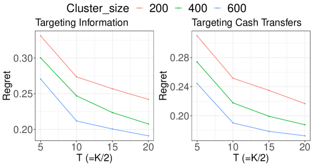
Figure H.1: Multi-wave experiment in Section 7. $200$ replications. In-sample regret, average across clusters, for $\rho=2$.

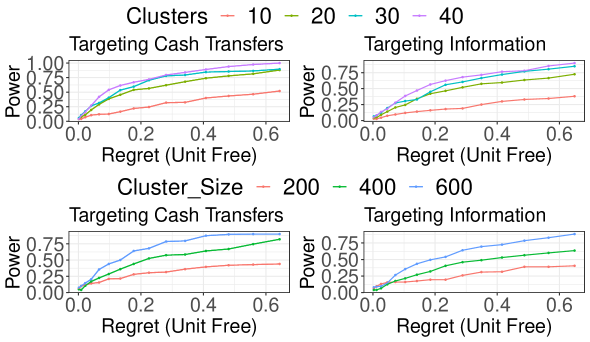
Figure H.2: One-wave experiment in Section 7. Power plot for $\rho=6$. The panels at the top fix $n=400$ and varies $K$. The panels at the bottom fix $K=20$ and vary $n$.

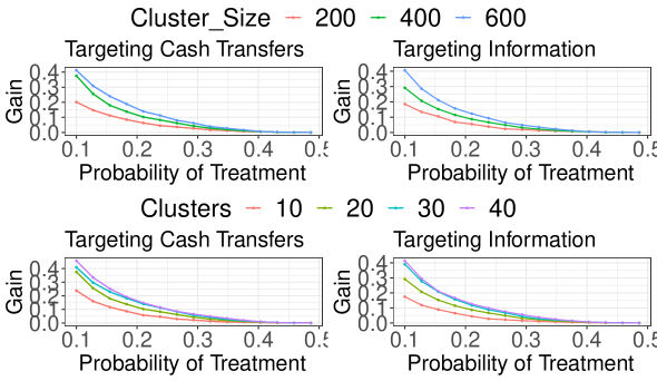
Figure H.3: One-wave experiment in Section 7. $\rho=6$. Expected percentage increase in welfare from increasing the probability of treatment $\beta$ by $5\%$ upon rejection of $H_{0}$. Here, the x-axis reports $\beta\in[0.1,\cdots,\beta^{*}-0.05]$. The panels at the top fix $n=400$ and varies the number of clusters. The panels at the bottom fix $K=20$ and vary $n$.

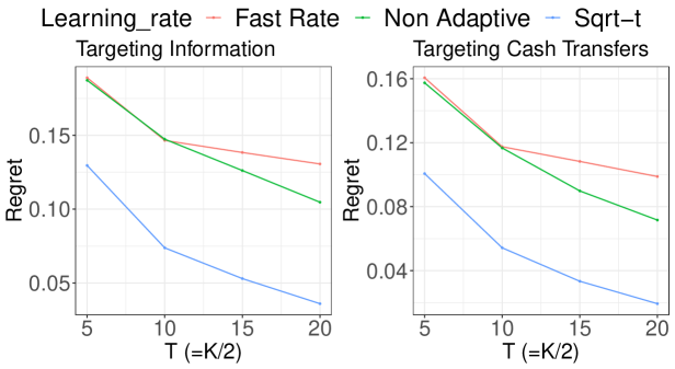
Figure H.4: Comparisons among different learning rates with experiment as in Section 7. 200 replications, $\rho=2,n=600,K=2T$. Fast rate denotes a rescaling of order $1/t$; non-adaptive depends on a rescaling of order $1/\sqrt{T}$; the last one (Sqrt-t) depends on a rescaling of order $1/\sqrt{t}$.

Table H.1: Multiple-wave experiment in Section 7. Relative improvement in welfare with respect to best competitor for $\rho=6$. The panel at the top reports the out-of-sample regret and the one at the bottom the worst case in-sample regret across clusters.

	Information							Cash Transfer
$T=$	5	10	15	20					5	10	15	20
$n=200$	$0.03$	$0.105$	$0.243$	$0.156$					$0.233$	$0.243$	$0.264$	$0.287$
$n=400$	$0.135$	$0.130$	$0.244$	$0.258$					$0.243$	$0.274$	$0.321$	$0.335$
$n=600$	$0.217$	$0.214$	$0.281$	$0.344$					$0.261$	$0.313$	$0.343$	$0.360$
$n=200$	$0.587$	$0.695$	$0.670$	$0.627$					$0.247$	$0.279$	$0.300$	$0.320$
$n=400$	$0.551$	$0.667$	$0.830$	$0.869$					$0.266$	$0.306$	$0.343$	$0.352$
$n=600$	$0.589$	$0.771$	$0.897$	$0.955$					$0.294$	$0.360$	$0.387$	$0.387$

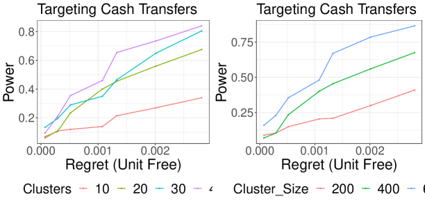
Figure H.5: Single-wave experiment in Section H.3. Power, 200 replications.

Table H.2: Single-wave experiment in Section H.3, 200 replications. Coverage for tests with size $5\%$.

$K=$	$10$	$20$	$30$	$40$
$n=200$	$0.955$	$0.935$	$0.900$	$0.905$
$n=400$	$0.965$	$0.945$	$0.900$	$0.950$
$n=600$	$0.935$	$0.965$	$0.920$	$0.965$

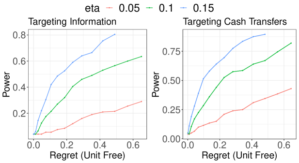
Figure H.6: One wave experiment calibrated to Alatas et al. (2012) and Cai et al. (2015). The plot reports power for different values of $\eta_{n}$ varies, with $K=200,n=400$, with 200 replications.

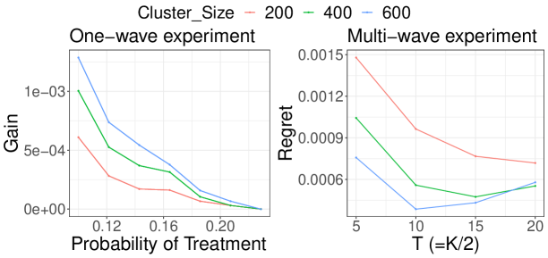
Figure H.7: Experiment in Section H.3. Left-hand side panel reports the expected percentage increase in welfare from increasing the probability of treatment $\beta$ by $5\%$ to individuals in remote areas upon rejection of $H_{0}$. Here, the x-axis reports $\beta\in[0.1,\cdots,\beta^{*}-0.05]$. The right-hand side panel reports the in-sample regret. 400 replications.

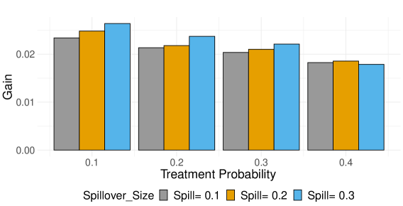
Figure H.8: One wave experiment in Section H.4. Relative welfare improvement for increasing the probability of treatment by ten percent, conditional on rejecting the null hypothesis. 200 replications. Different columns correspond to different levels of spillover effects (captured by $\alpha$). Here $K=20$.

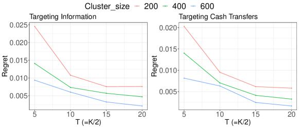
Figure H.9: Multi-wave experiment wave experiment in Section 7, as $\beta$ is initialized at the optimum value minus $5\%$. Reported in the figure is the out-of-sample welfare. 200 replications.

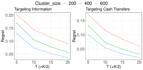
Figure H.10: Adaptive experiment $\rho=2$. $200$ replications. The panel reports the out-of-sample regret of the method as a function of the number of iterations.

References

- Abadie et al. (2017) Abadie, A., S. Athey, G. W. Imbens, and J. Wooldridge (2017). When should you adjust standard errors for clustering? Technical report, National Bureau of Economic Research.
- Adusumilli et al. (2019) Adusumilli, K., F. Geiecke, and C. Schilter (2019). Dynamically optimal treatment allocation using reinforcement learning. arXiv preprint arXiv:1904.01047.
- Agarwal et al. (2010) Agarwal, A., O. Dekel, and L. Xiao (2010). Optimal algorithms for online convex optimization with multi-point bandit feedback. In COLT, pp. 28–40. Citeseer.
- Akbarpour et al. (2018) Akbarpour, M., S. Malladi, and A. Saberi (2018). Just a few seeds more: value of network information for diffusion. Available at SSRN 3062830.
- Alatas et al. (2016) Alatas, V., A. Banerjee, A. G. Chandrasekhar, R. Hanna, and B. A. Olken (2016). Network structure and the aggregation of information: Theory and evidence from indonesia. American Economic Review 106(7), 1663–1704.
- Alatas et al. (2012) Alatas, V., A. Banerjee, R. Hanna, B. A. Olken, and J. Tobias (2012). Targeting the poor: evidence from a field experiment in indonesia. American Economic Review 102(4), 1206–40.
- Andrews et al. (2019) Andrews, I., T. Kitagawa, and A. McCloskey (2019). Inference on winners. Technical report, National Bureau of Economic Research.
- Armstrong and Shen (2015) Armstrong, T. and S. Shen (2015). Inference on optimal treatment assignments.
- Aronow and Samii (2017) Aronow, P. M. and C. Samii (2017). Estimating average causal effects under general interference, with application to a social network experiment. The Annals of Applied Statistics 11(4), 1912–1947.
- Athey and Imbens (2018) Athey, S. and G. W. Imbens (2018). Design-based analysis in difference-in-differences settings with staggered adoption. Technical report, National Bureau of Economic Research.
- Athey and Wager (2021) Athey, S. and S. Wager (2021). Policy learning with observational data. Econometrica 89(1), 133–161.
- Bai (2019) Bai, Y. (2019). Optimality of matched-pair designs in randomized controlled trials. Available at SSRN 3483834.
- Baird et al. (2018) Baird, S., J. A. Bohren, C. McIntosh, and B. Özler (2018). Optimal design of experiments in the presence of interference. Review of Economics and Statistics 100(5), 844–860.
- Banerjee et al. (2013) Banerjee, A., A. G. Chandrasekhar, E. Duflo, and M. O. Jackson (2013). The diffusion of microfinance. Science 341(6144), 1236498.
- Basse and Feller (2018) Basse, G. and A. Feller (2018). Analyzing two-stage experiments in the presence of interference. Journal of the American Statistical Association 113(521), 41–55.
- Basse and Airoldi (2018) Basse, G. W. and E. M. Airoldi (2018). Model-assisted design of experiments in the presence of network-correlated outcomes. Biometrika 105(4), 849–858.
- Bhattacharya et al. (2013) Bhattacharya, D., P. Dupas, and S. Kanaya (2013). Estimating the impact of means-tested subsidies under treatment externalities with application to anti-malarial bednets. Technical report, National Bureau of Economic Research.
- Bloch et al. (2019) Bloch, F., M. O. Jackson, and P. Tebaldi (2019). Centrality measures in networks. Available at SSRN 2749124.
- Bottou et al. (2018) Bottou, L., F. E. Curtis, and J. Nocedal (2018). Optimization methods for large-scale machine learning. Siam Review 60(2), 223–311.
- Breza et al. (2020) Breza, E., A. G. Chandrasekhar, T. H. McCormick, and M. Pan (2020). Using aggregated relational data to feasibly identify network structure without network data. American Economic Review 110(8), 2454–84.
- Brooks (1941) Brooks, R. L. (1941). On colouring the nodes of a network. In Mathematical Proceedings of the Cambridge Philosophical Society, Volume 37, pp. 194–197.
- Bubeck (2014) Bubeck, S. (2014). Convex optimization: Algorithms and complexity. arXiv preprint arXiv:1405.4980.
- Bubeck et al. (2012) Bubeck, S., N. Cesa-Bianchi, et al. (2012). Regret analysis of stochastic and nonstochastic multi-armed bandit problems. Foundations and Trends® in Machine Learning 5(1), 1–122.
- Cai et al. (2015) Cai, J., A. De Janvry, and E. Sadoulet (2015). Social networks and the decision to insure. American Economic Journal: Applied Economics 7(2), 81–108.
- Canay et al. (2017) Canay, I. A., J. P. Romano, and A. M. Shaikh (2017). Randomization tests under an approximate symmetry assumption. Econometrica 85(3), 1013–1030.
- Carneiro et al. (2010) Carneiro, P., J. J. Heckman, and E. Vytlacil (2010). Evaluating marginal policy changes and the average effect of treatment for individuals at the margin. Econometrica 78(1), 377–394.
- Chetty (2009) Chetty, R. (2009). Sufficient statistics for welfare analysis: A bridge between structural and reduced-form methods. Annu. Rev. Econ. 1(1), 451–488.
- Crépon et al. (2013) Crépon, B., E. Duflo, M. Gurgand, R. Rathelot, and P. Zamora (2013). Do labor market policies have displacement effects? evidence from a clustered randomized experiment. The quarterly journal of economics 128(2), 531–580.
- Duchi et al. (2018) Duchi, J., F. Ruan, and C. Yun (2018). Minimax bounds on stochastic batched convex optimization. In Conference On Learning Theory, pp. 3065–3162. PMLR.
- Duflo et al. (2023) Duflo, E., D. Keniston, T. Suri, and C. Zipfel (2023). Chat over coffee? diffusion of agronomic practices and market spillovers in rwanda. Technical report, National Bureau of Economic Research.
- D’Haultfœuille et al. (2023) D’Haultfœuille, X., S. Hoderlein, and Y. Sasaki (2023). Nonparametric difference-in-differences in repeated cross-sections with continuous treatments. Journal of Econometrics 234(2), 664–690.
- Egger et al. (2019) Egger, D., J. Haushofer, E. Miguel, P. Niehaus, and M. W. Walker (2019). General equilibrium effects of cash transfers: experimental evidence from kenya. Technical report, National Bureau of Economic Research.
- Fabregas et al. (2019) Fabregas, R., M. Kremer, and F. Schilbach (2019). Realizing the potential of digital development: The case of agricultural advice. Science 366(6471), eaay3038.
- Flaxman et al. (2004) Flaxman, A. D., A. T. Kalai, and H. B. McMahan (2004). Online convex optimization in the bandit setting: gradient descent without a gradient. arXiv preprint cs/0408007.
- Goldsmith-Pinkham and Imbens (2013) Goldsmith-Pinkham, P. and G. W. Imbens (2013). Social networks and the identification of peer effects. Journal of Business & Economic Statistics 31(3), 253–264.
- Graham et al. (2010) Graham, B. S., G. W. Imbens, and G. Ridder (2010). Measuring the effects of segregation in the presence of social spillovers: A nonparametric approach. Technical report, National Bureau of Economic Research.
- Hadad et al. (2019) Hadad, V., D. A. Hirshberg, R. Zhan, S. Wager, and S. Athey (2019). Confidence intervals for policy evaluation in adaptive experiments. arXiv preprint arXiv:1911.02768.
- Hazan et al. (2015) Hazan, E., K. Levy, and S. Shalev-Shwartz (2015). Beyond convexity: Stochastic quasi-convex optimization. In Advances in Neural Information Processing Systems, pp. 1594–1602.
- Hirano and Porter (2020) Hirano, K. and J. R. Porter (2020). Asymptotic analysis of statistical decision rules in econometrics. Handbook of Econometrics.
- Horvitz and Thompson (1952) Horvitz, D. G. and D. J. Thompson (1952). A generalization of sampling without replacement from a finite universe. Journal of the American statistical Association 47(260), 663–685.
- Hu et al. (2021) Hu, Y., S. Li, and S. Wager (2021). Average treatment effects in the presence of interference. arXiv preprint arXiv:2104.03802.
- Hudgens and Halloran (2008) Hudgens, M. G. and M. E. Halloran (2008). Toward causal inference with interference. Journal of the American Statistical Association 103(482), 832–842.
- Ibragimov and Müller (2010) Ibragimov, R. and U. K. Müller (2010). t-statistic based correlation and heterogeneity robust inference. Journal of Business & Economic Statistics 28(4), 453–468.
- Imai et al. (2009) Imai, K., G. King, and C. Nall (2009). The essential role of pair matching in cluster-randomized experiments, with application to the mexican universal health insurance evaluation. Statistical Science 24(1), 29–53.
- Jackson and Wolinsky (1996) Jackson, M. O. and A. Wolinsky (1996). A strategic model of social and economic networks. Journal of economic theory 71(1), 44–74.
- Janson (2004) Janson, S. (2004). Large deviations for sums of partly dependent random variables. Random Structures & Algorithms 24(3), 234–248.
- Johari et al. (2020) Johari, R., H. Li, I. Liskovich, and G. Weintraub (2020). Experimental design in two-sided platforms: An analysis of bias. arXiv preprint arXiv:2002.05670.
- Kasy (2016) Kasy, M. (2016). Partial identification, distributional preferences, and the welfare ranking of policies. Review of Economics and Statistics 98(1), 111–131.
- Kasy and Sautmann (2019) Kasy, M. and A. Sautmann (2019). Adaptive treatment assignment in experiments for policy choice. Econometrica.
- Kiefer and Wolfowitz (1952) Kiefer, J. and J. Wolfowitz (1952). Stochastic estimation of the maximum of a regression function. The Annals of Mathematical Statistics, 462–466.
- Kitagawa and Tetenov (2018) Kitagawa, T. and A. Tetenov (2018). Who should be treated? Empirical welfare maximization methods for treatment choice. Econometrica 86(2), 591–616.
- Kitagawa and Wang (2021) Kitagawa, T. and G. Wang (2021). Who should get vaccinated? individualized allocation of vaccines over sir network. Journal of Econometrics.
- Kleinberg (2005) Kleinberg, R. D. (2005). Nearly tight bounds for the continuum-armed bandit problem. In Advances in Neural Information Processing Systems, pp. 697–704.
- Laber et al. (2014) Laber, E. B., D. J. Lizotte, M. Qian, W. E. Pelham, and S. A. Murphy (2014). Dynamic treatment regimes: Technical challenges and applications. Electronic journal of statistics 8(1), 1225.
- Leung (2020) Leung, M. P. (2020). Treatment and spillover effects under network interference. Review of Economics and Statistics 102(2), 368–380.
- Leung (2021) Leung, M. P. (2021). Network cluster-robust inference. arXiv preprint arXiv:2103.01470.
- Li and Wager (2020) Li, S. and S. Wager (2020). Random graph asymptotics for treatment effect estimation under network interference. arXiv preprint arXiv:2007.13302.
- Lubold et al. (2020) Lubold, S., A. G. Chandrasekhar, and T. H. McCormick (2020). Identifying the latent space geometry of network models through analysis of curvature. Technical report, National Bureau of Economic Research.
- Manresa (2013) Manresa, E. (2013). Estimating the structure of social interactions using panel data. Unpublished Manuscript. CEMFI, Madrid.
- Manski (2004) Manski (2004). Statistical treatment rules for heterogeneous populations. Econometrica 72(4), 1221–1246.
- Manski (2010) Manski, C. F. (2010). Vaccination with partial knowledge of external effectiveness. Proceedings of the National Academy of Sciences 107(9), 3953–3960.
- Manski (2013) Manski, C. F. (2013). Identification of treatment response with social interactions. The Econometrics Journal 16(1), S1–S23.
- Manski (2017) Manski, C. F. (2017). Mandating vaccination with unknown indirect effects. Journal of Public Economic Theory 19(3), 603–619.
- Mbakop and Tabord-Meehan (2021) Mbakop, E. and M. Tabord-Meehan (2021). Model selection for treatment choice: Penalized welfare maximization. Econometrica 89(2), 825–848.
- Miguel and Kremer (2004) Miguel, E. and M. Kremer (2004). Worms: identifying impacts on education and health in the presence of treatment externalities. Econometrica 72(1), 159–217.
- Muandet et al. (2016) Muandet, K., K. Fukumizu, B. Sriperumbudur, and B. Schölkopf (2016). Kernel mean embedding of distributions: A review and beyond. arXiv preprint arXiv:1605.09522.
- Muralidharan and Niehaus (2017) Muralidharan, K. and P. Niehaus (2017). Experimentation at scale. Journal of Economic Perspectives 31(4), 103–24.
- Rai (2018) Rai, Y. (2018). Statistical inference for treatment assignment policies.
- Ross et al. (2011) Ross, N. et al. (2011). Fundamentals of stein’s method. Probability Surveys 8, 210–293.
- Sasaki and Ura (2020) Sasaki, Y. and T. Ura (2020). Welfare analysis via marginal treatment effects. arXiv preprint arXiv:2012.07624.
- Sävje et al. (2021) Sävje, F., P. M. Aronow, and M. G. Hudgens (2021). Average treatment effects in the presence of unknown interference. The Annals of Statistics 49(2), 673–701.
- Shamir (2013) Shamir, O. (2013). On the complexity of bandit and derivative-free stochastic convex optimization. In Conference on Learning Theory, pp. 3–24. PMLR.
- Sinclair et al. (2012) Sinclair, B., M. McConnell, and D. P. Green (2012). Detecting spillover effects: Design and analysis of multilevel experiments. American Journal of Political Science 56(4), 1055–1069.
- Stoye (2009) Stoye, J. (2009). Minimax regret treatment choice with finite samples. Journal of Econometrics 151(1), 70–81.
- Tabord-Meehan (2018) Tabord-Meehan, M. (2018). Stratification trees for adaptive randomization in randomized controlled trials. arXiv preprint arXiv:1806.05127.
- Vazquez-Bare (2017) Vazquez-Bare, G. (2017). Identification and estimation of spillover effects in randomized experiments. arXiv preprint arXiv:1711.02745.
- Viviano (2019) Viviano, D. (2019). Policy targeting under network interference. arXiv preprint arXiv:1906.10258.
- Viviano (2020) Viviano, D. (2020). Experimental design under network interference. arXiv preprint arXiv:2003.08421.
- Viviano et al. (2021) Viviano, D., K. Wuthrich, and P. Niehaus (2021). (when) should you adjust inferences for multiple hypothesis testing? arXiv preprint arXiv:2104.13367.
- Wager and Xu (2021) Wager, S. and K. Xu (2021). Experimenting in equilibrium. Management Science.
- Wainwright (2019) Wainwright, M. J. (2019). High-dimensional statistics: A non-asymptotic viewpoint, Volume 48. Cambridge University Press.
- Zhang et al. (2020) Zhang, K., L. Janson, and S. Murphy (2020). Inference for batched bandits. Advances in neural information processing systems 33, 9818–9829.