A Demonstration of Improved Constraints on Primordial Gravitational Waves with Delensing

Abstract

We present a constraint on the tensor-to-scalar ratio, $r$, derived from measurements of cosmic microwave background (CMB) polarization $B$-modes with “delensing,” whereby the uncertainty on $r$ contributed by the sample variance of the gravitational lensing $B$-modes is reduced by cross-correlating against a lensing $B$-mode template. This template is constructed by combining an estimate of the polarized CMB with a tracer of the projected large-scale structure. The large-scale-structure tracer used is a map of the cosmic infrared background derived from Planck satellite data, while the polarized CMB map comes from a combination of South Pole Telescope, Bicep/Keck, and Planck data. We expand the Bicep/Keck likelihood analysis framework to accept a lensing template and apply it to the Bicep/Keck data set collected through 2014 using the same parametric foreground modelling as in the previous analysis. From simulations, we find that the uncertainty on $r$ is reduced by $\sim 10\%$, from $\sigma(r)$= $0.024$ to $0.022$, which can be compared with a $\sim 26\%$ reduction obtained when using a perfect lensing template or if there were zero lensing $B$-modes. Applying the technique to the real data, the constraint on $r$ is improved from $r_{0.05}<0.090$ to $r_{0.05}<0.082$ (95% C.L.). This is the first demonstration of improvement in an $r$ constraint through delensing.

I Introduction

Inflation describes a period of near-exponential expansion during the earliest moments of the universe. The inflationary paradigm provides conceptual solutions to problems arising from the Big Bang description of the early universe including the horizon problem and the flatness problem. Furthermore, inflationary models make testable predictions about perturbations away from perfect homogeneity and isotropy kamionkowski2016 . These predictions have been confirmed in observations of the cosmic microwave background (CMB) temperature and polarization anisotropies. They include the Gaussianity, phase-synchronicity, and near-scale-invariance of the scalar density fluctuations, and super-horizon correlation of the CMB anisotropies planck2018inflation . However, one prediction from inflation that has yet to be confirmed is the existence of a stochastic primordial gravitational wave (PGW) background.

PGWs are generically predicted in many inflationary models. Their amplitude is parametrized by $r$, the ratio of the amplitudes of the tensor and scalar perturbation spectra at a pivot scale ($k_{*}=0.05$ Mpc^-1 in this work). If PGWs exist, they would imprint a specific divergence-free ($B$-mode) signature in the polarization of the CMB seljak97 ; kamion97 . This makes CMB polarization a promising avenue in the search for PGWs.

However, PGWs are not the only source of $B$-modes. Thermal dust and synchrotron emission within our galaxy produce polarized foreground patterns which contain $B$-modes planckintXXX ; spass18 . Additionally, there is a source of $B$-modes, called the “lensing $B$-mode,” produced by gravitational lensing of the CMB lewis2006 . If there were no inhomogeneities in the matter between us and the last scattering surface, then scalar perturbations from inflation would produce a purely curl-free ($E$-mode) CMB polarization pattern. However, during their propagation to us, the polarized CMB photons undergo small gravitational deflections by the forming large-scale structure along the line of sight. This produces a $B$-mode component which is small compared to the source $E$-modes, and which has already been detected by a number of experiments Hanson:2013hsb ; polarbearbb14 ; keisler15 ; louis16 ; bk6 ; polarbearbb17 ; bk10 .

The Bicep/Keck experiments have deployed CMB polarization telescopes optimized for measurements at the “recombination bump” in the predicted PGW-generated B-mode spectrum (harmonic multipoles $\ell\sim 80$, or angular scales of $\sim 2$ degrees). To separate out the Galactic dust and synchrotron components, which have different frequency spectral shapes than the black-body emission of the CMB, Bicep/Keck observes in several frequency bands, and the $r$ analyses also incorporate maps at additional frequencies from the WMAP and Planck satellites. The existing analysis pipeline takes all possible auto- and cross-spectra of the maps at different frequencies and compares these against a parametric model of CMB and foregrounds bk6 ; bk10 to set constraints on $r$ which are close to optimal given the available data. Alternative approaches involving “cleaning coefficient” subtraction of a dust template map (as measured at a higher frequency) would in general be less powerful (e.g. bkp, ).

In contrast to the foregrounds, the lensing component has the same frequency spectral shape as the PGW component, and thus cannot be constrained using multi-frequency observations. Given an estimate of the projected gravitational potential responsible for CMB lensing and the observed CMB $E$-mode pattern, one can estimate the $B$-modes which have been produced by the lensing effect. Subtracting these from the observed $B$-modes has been demonstrated to reduce $B$-mode power in several recent works manzotti17 ; carron17 ; plancklens18 ; pbdelens19 ; actdelens20 . However, none of these works have demonstrated a reduction in the $B$-mode measurement uncertainties at large angular scales—a necessary step to achieve improved constraints on PGWs. This subtraction process is usually referred to as “delensing.” But in this work, we take a different approach and therefore broaden the meaning of delensing to include any process which reduces the effective lensing sample variance in the $B$-mode measurements. Specifically, we extend the Bicep/Keck analysis pipeline to accept an estimate of the lensing $B$-modes as a “lensing template”—an additional pseudo-frequency band against which cross-spectra are taken. This (optimally) reduces the effective sample variance of the lensing $B$-mode component, and hence reduces the uncertainty of the PGW contribution.

The lensing potential $\phi$ can be computed using higher-order statistics of the CMB pattern itself huokamoto02 . However, since the lensing potential is a weighted integral of the mass distribution along the line of sight between us and the last scattering surface, we may also approximate it by other tracers of this mass distribution. At the noise levels of current CMB observations, it turns out to be better to use a cosmic infrared background (CIB) simard15 ; sherwin15 map rather than one of the available CMB lensing reconstructions plancklens18 ; wu2019 directly. To use an alternate tracer of $\phi$, we need to know the degree of correlation between it and the true CMB lensing potential—if this were misestimated it could potentially lead to a false detection of PGW. This correlation may be found empirically from the cross-correlation of the tracer with a reconstruction of the CMB lensing potential. In this paper, we use a CIB map from Planck generated using the Generalized Needlet Internal Linear Combination (GNILC) component separation algorithm planck2015cibdust as the $\phi$ tracer and estimate its correlation with the lensing potential using a Planck minimum-variance lensing map plancklens15 .

To estimate the lensing template, in addition to the tracer of the lensing potential, one also needs the best available estimate of the observed CMB polarization pattern. Since the lensing operation mixes modes over a wide range of angular scales, the inclusion of small-scale $E$-modes is important for precise estimation of the lensing $B$-modes at the angular scales of interest ($\ell\sim 80$). Therefore, we use arcminute-resolution maps from the South Pole Telescope (SPT) second-generation camera SPTpol, augmenting these with polarization measurements from Bicep/Keck and Planck.

In this paper, we add the CIB-derived lensing template to the previous “BK14” analysis (bk6, ) which utilizes data from Bicep/Keck through the 2014 observation season. With the addition of the lensing template, we demonstrate a $\sim 10\%$ reduction in the uncertainty on $r$ for the BK14 data set, to be compared with a $\sim 26\%$ reduction in the uncertainty on $r$ when using a perfect lensing template or if there were zero lensing $B$-modes. This shows that the lensing sample variance is a subdominant fraction of the uncertainty on $r$ for BK14. However, it will be an increasingly limiting factor going forward. Therefore, this analysis serves as a proof of principle, and a first step towards future analyses where delensing will more significantly improve $\sigma(r)$.

This paper is organized as follows: In Sec. II, we describe the construction of the lensing template and the extension to the Bicep/Keck pipeline to include the lensing template. In Sec. III, we describe the data and simulation sets of the CMB maps, how we combine the $Q/U$ maps from SPTpol, Bicep/Keck, and Planck, and the data and simulations of the $\phi$ tracer. We validate our simulations and pipeline in Sec. IV and test for systematics in Sec. V. We present our results in Sec. VI and conclude in Sec. VII.

II Method

In this section, we describe new elements added to the Bicep/Keck analysis framework to incorporate information on the lensing $B$-modes in the Bicep/Keck patch, with the aim of reducing the effective uncertainty of the observed $B$-modes, and thereby reducing the uncertainty on $r$. We illustrate the incorporation of the lensing template into the Bicep/Keck likelihood analysis framework schematically in Fig. 1. There are two main areas of new development: (1) constructing a lensing template, and (2) extending the Bicep/Keck pipeline to include the lensing template. We will describe each aspect in the following subsections.

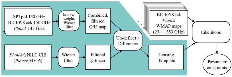
Figure 1: Schematic of the analysis flow in this work. The rectangular blocks denote input maps; the blocks with rounded corners denote operations on maps. The teal-colored region highlights the inputs to, and processes involved in generating, the lensing template. The input maps include the SPTpol, Bicep/Keck, and Planck $Q/U$ maps, the Planck GNILC CIB map, and the Planck minimum-variance (MV) reconstruction of $\phi$. The Planck MV $\phi$ is in parentheses because, instead of using it as a $\phi$ tracer, we use it to filter and normalize the CIB map and for generating simulations. The unshaded region denotes the standard Bicep/Keck $r$ analysis, where auto- and cross-spectra of multi-frequency maps from Bicep/Keck, Planck, and WMAP form the input data for computing likelihoods to extract parameter constraints. The lensing template is injected into the standard analysis as an additional pseudo-frequency band.

II.1 Constructing the lensing template

The key element to constraining the lensing $B$-modes in the Bicep/Keck patch is making an estimate of these modes. To do this, we use two inputs: (1) a tracer of the CMB lensing potential $\phi$ from large-scale structure observations and (2) observed $Q/U$ polarization maps. We construct the lensing template using an “undeflect-and-difference” method in which we undeflect the observed $Q/U$ maps using the $\phi$ tracer and subtract the undeflected maps from the input.

Formally, we take the lensed, polarized CMB fields $\tilde{X}$, which are related to the unlensed CMB fields $X$ by

$$\tilde{X}_{\pm}(\hat{n})=X_{\pm}(\hat{n}+\nabla\phi(\hat{n}))$$ (1)

where $X_{\pm}=(Q\pm iU)$ and $\nabla\phi$ denotes the deflection field hu2000 . We undo the deflection by remapping the $\tilde{Q}$ and $\tilde{U}$ polarization fields by $-\nabla\phi$, evaluated at the lensed positions $\hat{n}^{\prime}$ (not delensed positions $\hat{n}$),

$$X^{d}_{\pm}(\hat{n})=\tilde{X}_{\pm}(\hat{n}^{\prime}),$$ (2)

where $\hat{n}^{\prime}=\hat{n}-\nabla\phi(\hat{n}^{\prime})$ and $X^{d}$ denotes the undeflected field. Therefore,

$$X_{\pm}(\hat{n})=X^{d}_{\pm}(\hat{n})=\tilde{X}_{\pm}(\hat{n}-\nabla\phi({\hat{n}}-\nabla\phi({\hat{n}-...})))$$ (3)

where the last expression is used for the practical implementation, and $...$ denotes the recursion that locates the position to which the value at $\hat{n}$ was deflected from the unlensed plane.

Specifically, the undeflection is implemented by first computing the amount of deflection at the lensed positions, denoted by ($dx,dy$), on the delensed map pixel grid $(x,y)$. To do that we first evaluate $\nabla\phi$ at $(x,y)$ to get ($dx^{\prime},dy^{\prime}$), and then we evaluate $\nabla\phi$ at $(x-dx^{\prime},y-dy^{\prime})$, and so on. We find that the solution converges after 1 recursion, which means that with the notation given, ($dx,dy$) is $\nabla\phi$ at $(x-dx^{\prime},y-dy^{\prime})$. The evaluation of $\nabla\phi$ at any grid point is done by interpolating $\nabla\phi$ values in Healpix format using first-order Taylor expansion. We then remap the $\tilde{Q}/\tilde{U}$ map pixels at ($x-dx,y-dy$) to ($x,y$) via cubic interpolation. We note that by evaluating the deflection field at the lensed positions, we do not incur the small $\mathcal{O}(\nabla\phi\cdot\nabla)\nabla\phi$ error found in similar algorithms that evaluate $\nabla\phi$ at the delensed positions anderes15 ; green16 ; carron17 .

The lensing templates $Q^{t}/U^{t}$ are then derived by subtracting the obtained undeflected map from the observed (lensed) one:

$$Q^{t}(\hat{n}) =\tilde{Q}(\hat{n})-Q^{d}(\hat{n})$$ (4)

$$U^{t}(\hat{n}) =\tilde{U}(\hat{n})-U^{d}(\hat{n}).$$ (5)

We test the algorithm on noiseless lensed simulations using the $\phi$ maps which were used to lens them. The correlation of the resulting lensing $B$-mode template with the difference of the lensed and unlensed input skies is $\gtrsim 95\%$ for the angular scales used in this analysis. This is sufficiently accurate at the current noise levels. In other work, lensing templates have also been constructed after transforming to harmonic space, converting to $E/B$, and lensing by a $\phi$ tracer using expressions derived from the first-order Taylor expansion of Eq. 1 plancklens18 ; manzotti17 ; pbdelens19 . At the noise levels of the current analysis, the two approaches perform similarly in constraining the lensing $B$-mode contribution to the observed $B$-modes. We discuss in more detail the differences of the two approaches in Appendix A.

Since the undeflect-and-difference operation corresponds to an all-with-all mixing in Fourier space, to obtain the lowest possible lensing template noise in the $\ell$ range of interest we first Wiener filter (e.g. green16, ) the $Q/U$ and $\phi$-tracer maps. We filter the $Q/U$ maps by a 2D Wiener filter in Fourier space

$$\tilde{Q}(\boldsymbol{\ell}) \rightarrow\frac{C_{\boldsymbol{\ell}}^{EE}}{C_{\boldsymbol{\ell}}^{EE}+N_{\boldsymbol{\ell}}^{EE}}\,\tilde{Q}(\boldsymbol{\ell}),$$ (6)

$$\tilde{U}(\boldsymbol{\ell}) \rightarrow\frac{C_{\boldsymbol{\ell}}^{EE}}{C_{\boldsymbol{\ell}}^{EE}+N_{\boldsymbol{\ell}}^{EE}}\,\tilde{U}(\boldsymbol{\ell}),$$ (7)

to account for anisotropic noise and mode-loss due to filtering. $C_{\boldsymbol{\ell}}^{EE}$ and $N_{\boldsymbol{\ell}}^{EE}$ are 2D power spectra of the $E$-mode signal and noise components, constructed from a weighted combination of $Q/U$ maps from the three experiments SPTpol, Bicep/Keck, and Planck. We describe the procedure to combine the $Q/U$ maps and the details of the Wiener filter in Sec. III.1.3.

We filter and normalize the $\phi$ tracer in spherical harmonic space according to

$$\phi^{\rm\cal{T}}_{LM}=\left(\frac{C_{L}^{\rm\cal{T}\phi^{\prime}}}{C_{L}^{\rm\cal{T}\cal{T}}}\right){\cal T}_{LM},$$ (8)

where $\cal{T}$ denotes the tracer and $\phi^{\prime}$ is an unbiased, but noisy map of the true CMB lensing potential (simard15, ; sherwin15, ). To see that this weighting is a joint normalization and Wiener filter, we write ${\rm\cal{T}}_{LM}=g_{L}\phi_{LM}+n_{LM}$, where $g_{L}$ is the relative normalization factor (and unit conversion), $\phi$ is the true (noiseless) lensing potential, and $n$ is the effective noise in the tracer pattern (the part which does not correlate with $\phi$) with power spectrum $N_{L}^{\cal{TT}}$. Expanding and taking the expectation value, we get

$$\frac{C_{L}^{\rm\cal{T}\phi^{\prime}}}{C_{L}^{\rm\cal{T}\cal{T}}}=\frac{g_{L}C_{L}^{\phi\phi}}{g_{L}^{2}C_{L}^{\phi\phi}+N_{L}^{\rm\cal{TT}}}=g_{L}^{-1}\frac{C_{L}^{\phi\phi}}{C_{L}^{\phi\phi}+N_{L}^{\rm\cal{TT}}/g_{L}^{2}},$$ (9)

fulfilling its role of normalization and filtering. In this paper the tracer $\cal{T}$ is a CIB map from Planck and $\phi^{\prime}$ is a lensing reconstruction map also from Planck—see Sec. III.2 below for further details.

With the $Q/U$ lensing templates constructed, we then take them as an additional pseudo-frequency band for input into the existing Bicep/Keck analysis.

II.2 Adding the lensing template to the existing analysis framework

The development of the existing Bicep/Keck $r$ analysis framework has been described in a series of papers bk1 ; bkp ; bk6 ; bk10 . Briefly, we take all possible auto- and cross-power spectra between the available frequency bands, and then compare the resulting set of bandpowers to their expectation values under a parametric model of lensed-$\Lambda$CDM+dust+synchrotron+$r$ using an expansion of the Hamimeche-Lewis likelihood approximation hl2008 . It is a straightforward extension to this framework to include the lensing template as an additional pseudo-frequency band. To do this we require reliable simulations of the signal and noise content of the lensing template so that we can (1) debias its auto-spectrum, (2) determine the expectation values of the auto- and cross-spectra involving the lensing template, and (3) determine the variance of these bandpowers, and their covariance with other bandpowers. These simulations are described in Sec. III below. Here we describe a few complications with respect to the normal procedure which arise in the steps above.

The lensing template is formed from two kinds of input maps (the $Q/U$ maps and the $\phi$ tracer) which both contain relevant amounts of noise. The Planck CIB map has very high signal-to-instrumental-noise. However, the integrated dust emission from star-forming galaxies back to the last scattering surface weights differently over redshift than the deflection of CMB photons, and these galaxies do not perfectly trace the underlying mass density field. This means that the CIB only partially correlates with the true lensing potential. For the purposes of this paper, the $\phi$ tracer signal is the portion of the CIB that is correlated with the true lensing potential $\phi$; the $\phi$ tracer noise corresponds to the uncorrelated portion. We detail our $\phi$ tracer simulations in Sec. III.2.2.

We remove the noise bias of the lensing template auto-spectrum by subtracting the noise auto-spectrum estimated from simulations. Schematically, the lensing template $B$-mode auto-spectrum is

$$\begin{split}\left<L_{B}^{2}\right>=&\left<((s_{QU}+n_{QU})\ast(s_{\phi}+n_{\phi}))^{2}\right>\\ =&\left<(s_{QU}\ast s_{\phi})^{2}\right>+\left<(s_{QU}\ast n_{\phi})^{2}\right>+\\ &\left<(n_{QU}\ast s_{\phi})^{2}\right>+\left<(n_{QU}\ast n_{\phi})^{2}\right>,\end{split}$$ (10)

where $s_{X}$ and $n_{X}$ denote the signal and noise components of field $X\in[QU,\phi]$ and $\ast$ denotes the following steps: undeflect-and-difference, Fourier transform, and convert from $Q/U$ to $B$-modes. In writing the second line, we have assumed all the cross terms have zero expectation value. We estimate the noise auto-spectrum from simulations as

$$\left<(n_{QU}\ast(s_{\phi}+n_{\phi}))^{2}\right>+\left<(s_{QU}\ast n_{\phi})^{2}\right>$$ (11)

averaged over all simulation realizations and subtract it from Eq. 10. The $Q/U$ and $\phi$ input signal and noise maps are Wiener filtered in the same way as the data maps (and the simulation signal+noise maps). Empirically, when adding this inferred noise bias to the mean of the signal-only simulation spectra ($Q/U$ signal undeflected with $\phi$ tracer signal) one obtains the mean of the signal+noise simulation spectra ($Q/U$ signal+noise undeflected with $\phi$ tracer signal+noise) to high fractional precision.

In the Bicep/Keck standard procedure, the filter/beam suppression of the bandpower values is computed using sets of maps which each contains power at only a single multipole $\ell$ passed through the “observing matrix” as described in Sec. VI.C of bk1 . However, since the lensing template is derived in a very different manner to the standard Bicep/Keck maps, the usual observing matrix is not applicable, and we fall back to a simulation-based approach. We rescale both the data and simulation lensing template auto- and cross-spectra by the ratio of the input lensing spectrum $C_{\ell}^{BB}$ to the average of the signal-only simulation bandpowers. This step overrides the normalization part of Eq. 9 applied to the $\phi$ tracer. However, accurate knowledge of the degree of correlation between the lensing tracer and the true lensing potential is still required to avoid bias on $r$ (see Sec. IV).

In the standard Bicep/Keck procedure, the bandpower covariance matrix is constructed by taking the auto- and cross-spectra of the signal and noise components of the simulations as described in Appendix H of bk10 . Since the lensing template is formed from two maps which both have signal and noise components we expand the usual procedure to form additional cross spectra and combine the results appropriately.

With this extended analysis framework, we can now incorporate lensing templates constructed using simulations and data to the Bicep/Keck likelihood and constrain the model parameters.

III Data and Simulations

The Bicep/Keck analysis pipeline relies on signal-only, noise-only, and signal+noise simulations, the construction of which is described in Sec. V of bk1 . We reuse the data maps and simulations including Gaussian realizations of Galactic dust from the BK14 analysis unchanged. The data maps include the WMAP and Planck bands with Bicep/Keck filtering applied (as described in Sec. II.A of bkp ). To add the lensing template as an additional pseudo-frequency band, we need data maps and corresponding simulations of it. Since the lensing template is constructed from $Q/U$ CMB maps and a CIB $\phi$ tracer, we in turn need data maps and simulations of both of these. As a pre-step, we combine the SPTpol, Bicep/Keck, and Planck $Q/U$ maps to generate a synthetic map which has the best possible signal-to-noise at all points in the 2D Fourier plane. Fig. 1 gives a schematic view of the steps involved in generating the various maps.

III.1 $Q/U$ CMB maps

Below we describe the data processing of the SPTpol, Bicep/Keck, and Planck $Q/U$ maps that are relevant in the construction of the combined $Q/U$ maps and their Wiener filter. The combined, Wiener filtered $Q/U$ maps are the inputs to the undeflect-and-difference step which is used to construct the lensing template.

III.1.1 Data CMB maps

SPTpol  maps: We use SPTpol maps made specifically for this analysis using 150 GHz observations taken between 2013 and 2015 by the SPTpol camera austermann12 on the South Pole Telescope carlstrom11 . The SPTpol 500 deg² survey field is centered at RA 0h and Dec. $-57.5^{\circ}$, matching the Bicep/Keck field. The polarization map depth is $\sim 10\,\mu$K arcmin in the multipole range of $300\lesssim\ell\lesssim 2000$. The time stream processing is identical to that in henning18 , except for the polynomial-filter order and the low-pass filter. We fit and subtract a third-order/sixth-order polynomial from the time stream of each detector over the RA extent of the lead-trail/full-field observations. We choose the low-pass filter based on the pixel size. This set of SPTpol maps is binned into 5 arcminute-sized pixels, which are a $\times 3$ resolution superset of the Bicep/Keck map pixels. To reduce aliasing given the pixel size, we apply a low-pass filter to the time stream that corresponds to $\ell\sim 1900$. The polarization maps, in addition to the calibration factors included through calibrating the temperature map against Planck, have an extra polarization calibration factor ($P_{cal}$) applied. The polarization calibration factor is taken from henning18 and is obtained by forming a cross-spectrum between the SPTpol $E$-mode map and an $E$-mode map from Planck. We discuss impacts on $r$ from biases in $P_{cal}$ in Sec. V.

Bicep/Keck maps: We use the Bicep2/Keck 150 GHz band $Q/U$ maps from BK14. These have noise of $\sim~{}3\,\mu$K arcmin over an effective area of 395 deg² centered at RA 0h, Dec. $-57.5^{\circ}$. The Bicep2 and Keck Array telescopes have $\sim$30 arcminute resolution at 150 GHz. This limits the highest angular multipole to which they are sensitive to $\ell$ of hundreds. As described in Sec. III & IV of bk1 the construction of the maps involves time-stream filtering. Specifically, a third-order polynomial was subtracted from the time streams of each detector over each scan. Across the $\sim\,$30^∘ scan throw on the sky, this approximately corresponds to removing $\ell_{x}<20$ modes. These maps are binned in 0.25^∘ rectangular pixels in RA and Dec, and calibrated by forming cross-spectra with the Planck temperature map.

Planck maps: We use the 143 GHz $Q/U$ “full mission” maps from Planck public release 2 as the input to the combined three-experiment $Q/U$ maps. We convert the map to $a_{\ell m}$, apply an anti-aliasing filter by low-pass filtering at $\ell=2100$, render a $N_{\rm side}=2048$ Healpix map, and interpolate to the same 5-arcminute pixel grid as used for the SPTpol maps.

III.1.2 Simulated CMB maps

We reuse the BK14 simulated maps unchanged. We thus need to make corresponding simulations for the SPTpol and Planck maps. The Bicep/Keck CMB sky realizations have remained the same since originally described in Sec. V of bk1 . These are the unlensed $a_{\ell m}$, Gaussian realizations of $\phi$ given the input cosmology, and lensed $a_{\ell m}$ generated using LensPix. The Bicep/Keck simulations were originally generated with a maximum $\ell$ of 1536 which is adequate given the beam sizes of the telescopes. To match more closely the pixel scale of the SPTpol and Planck maps in this analysis, we generate additional higher-$\ell$ $a_{\ell m}$, graft these onto the existing unlensed values, pass through LensPix, and graft the output onto the existing lensed values. Since lensing to some degree mixes angular scales this is clearly only approximately correct, but we note that the amount of lensing $B$-modes below $\ell$ of 350 sourced from $E$-modes between $\ell$ of 1536 and 2100 (the pixel-scale) is negligible (see e.g. Fig. 2 of simard15, ). We refer to this set of input lensed and unlensed $a_{\ell m}$ as the extended set and the original set as the standard set.

We generate SPTpol simulations for this analysis using the extended set of $a_{\ell m}$. In a procedure similar to that used to generate the existing Bicep/Keck simulations, we multiply the input $a_{\ell m}$ by the instrument beam, “mock-observe” the skies by creating time-stream samples given the pointing information of each detector, apply the same time-stream level filters as applied to data, and bin to maps in the pixelization used for the real data. Corresponding noise realizations are generated by the standard method used in both Bicep/Keck and SPT analyses—differencing combinations of halves of data maps, where the halves are defined so that the weights of each half are close to equal.

We generate simulated maps for Planck 143 GHz by first taking the $a_{\ell m}$ from the extended set and multiplying them by the Planck 143 GHz beam. We then low-pass filter and process as for the real Planck map. Corresponding noise realizations are taken from the Planck FFP8 simulations and processed identically to the real Planck map. We generate 499 realizations of signal and noise skies for each experiment as is the Bicep/Keck standard.

III.1.3 Combining and Filtering the $Q/U$ maps from SPTpol, Bicep/Keck, and Planck

A factor that impacts the delensing efficiency (the recovery of the lensing $B$-modes) is the per-mode noise of the input $Q/U$ maps. The lower the noise per mode, the better the lensing templates trace the true lensing $B$-modes. The lensing $B$-modes at multipole $\ell$ are mostly sourced by $E$-modes from a range of multipoles slightly higher in $\ell$ (smaller in angular scale) (see e.g. Fig. 2 of simard15, ). Bicep/Keck does not image these smaller-scale $E$-modes very well because of its large beam size. Therefore, it is advantageous to combine with polarization measurements from other, higher-resolution experiments such as SPTpol and Planck to increase the signal-to-noise ratio of the input $Q/U$ maps, and thus the $E$-modes.

We combine the three maps in Fourier space. We divide from the 2D mode sets of the three experiments their respective 2D transfer functions, taken as the square-root of the mean of the 2D $E$-mode power spectra of the signal-only simulations divided by the mean of the corresponding spectra of the (unfiltered) input maps. We also divide the 2D noise power spectra by the same ratio (without the square root). We then combine the SPTpol, Bicep/Keck, and Planck $Q/U$ modes using an inverse-variance weighting taken from the mean of the 2D noise power spectra. Specifically, the combined $Q/U$ mode sets are

$${\cal X}(\boldsymbol{\ell})=\sum_{i}w_{i}(\boldsymbol{\ell}){\cal X}_{i}(\boldsymbol{\ell}),$$ (12)

where ${\cal X}\in[Q,U]$, $i\in$ [ SPTpol, Bicep/Keck, Planck ], and $w_{i}$ denotes the weight

$$w_{i}(\boldsymbol{\ell})=\frac{N^{-1}_{i}(\boldsymbol{\ell})}{\sum_{i}N^{-1}_{i}(\boldsymbol{\ell})}.$$ (13)

Here, $N_{i}(\boldsymbol{\ell})$ denotes the mean of the transfer-function-divided 2D angular power spectra of the $E$-mode noise realizations from experiment $i$. We additionally impose $\ell_{x}$ cuts by artificially increasing the noise below some $\ell_{x}$ to remove modes that are empirically found to be unrecoverable due to the scan-wise timestream filtering. We set $\ell_{x}$ to 25 for Bicep/Keck and $\ell_{x}$ to 50 for SPTpol.

Before passing the combined $Q/U$ map to the lensing template construction step, we apply a Wiener filter as described in Sec. II.1 above. The $C_{\boldsymbol{\ell}}^{EE}$ in Eq. 6 is the 2D input $E$-mode power spectrum and the $N_{\boldsymbol{\ell}}^{EE}$ of the combined modes is

$$N^{EE}_{\boldsymbol{\ell}}=\sum_{i}w^{2}_{i}(\boldsymbol{\ell})N_{i}(\boldsymbol{\ell}),$$ (14)

with $w_{i}(\boldsymbol{\ell})$ given by Eq. 13.

In the above, we transform to Fourier space and back again, and hence need to choose an apodization mask. Due to the small instantaneous field of view of the SPTpol camera as compared to the size of the observation region, the integration time map (inverse noise variance map) is a near uniform rectangular box tapering to zero over a few degrees at the edges. In contrast, the Bicep/Keck integration time map has no uniform central region and tapers smoothly and continuously from a peak in the middle (see for instance Fig. 1 of bkp ), with non-zero coverage extending well outside the SPTpol region. (Planck observes the full sky and has close to uniform coverage across the sky region in question.) To perform the map combination we need to pick a single apodization function for all three input maps. We choose to use the one built from the SPTpol integration time map, with a cosine taper with radius of 1 degree. This is because SPTpol is the experiment with the most restrictive sky coverage, but the best mode coverage. This means that the resulting lensing template does not cover the full Bicep/Keck sky region. In addition, because of the chosen spatial weighting of pixels, we introduce sub-optimality in the combination.

Fig. 2 illustrates the process. The left three panels show the 2D $E$-mode signal power spectra for the three experiments. We see the $\Lambda$CDM $E$-mode spectrum rolled-off by the beam window function of each telescope. Because of their scan strategies and the applied scan-wise filtering, Bicep/Keck and SPTpol have filtered out the modes along the $\ell_{y}$ axis; while Planck has isotropic mode coverage. The right panel shows the combined mode set after the final Wiener filter step, so only modes measured with good signal-to-noise are retained. At $\ell>500$ Planck does not have good per-mode signal-to-noise so the modes along the $\ell_{y}$ axis beyond this multipole cannot be filled in.

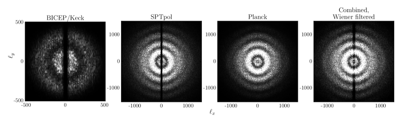
Figure 2: Simulated 2D $E$-mode signal power spectra of Bicep/Keck, SPTpol, and Planck. The axis scales for the Bicep/Keck Fourier plane are zoomed in compared with the rest of the panels to focus on the modes accessible by Bicep/Keck’s small apertures. The color stretch in all four panels is identical. For Bicep/Keck and SPTpol  because the observations are being made at the South Pole with scans along the azimuth direction, scan-wise filtering leads to modes along the $\ell_{y}$ axis being suppressed. These filtered modes along the $\ell_{y}$ axis can be partially filled in using measurements from Planck. To generate the combined, Wiener filtered 2D $E$-mode signal power spectra on the rightmost panel, the three sets of modes to the left are corrected for beam and filtering, combined using inverse-noise weighting, and Wiener filtered to suppress modes which remain noisy in the combined set (as described in Sec. III.1.3). We see that some modes remain unavailable for lensing template construction at $|\ell_{x}|<100$ and $|\ell_{y}|>500$.

We next proceed to inverse-Fourier transform the combined and Wiener filtered $Q/U$ modes back to image space where they are ready to be undeflected by the gradient of the $\phi$ tracer. The $Q/U$ maps at this stage are shown in the top panels of Fig. 3.

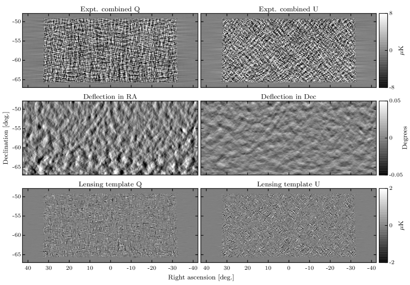
Figure 3: The top two panels show the experiment-combined and Wiener filtered $Q/U$ maps. The middle two panels show the $x$ and $y$ derivatives of the normalized and Wiener filtered Planck CIB map. Signal and noise are approximately equal in these maps. Due to the foreshortening effect the RA deflections are larger and increase towards more negative Dec. The $Q/U$ maps in the top panels are undeflected by the angles shown in the middle panels and differenced with the initial maps to form the lensing template $Q/U$ maps shown in the bottom panels.

III.2 CIB map

With the combined and filtered $Q/U$ maps in hand, we next need a $\phi$ tracer map. In the following, we describe the characteristics of the CIB map used in this analysis, and how we generate simulations of it in the Bicep/Keck patch.

III.2.1 CIB data

It is possible to reconstruct the lensing potential field $\phi$ from the CMB temperature and polarization patterns plancklens18 , and in the future this will become the best $\phi$ estimate for delensing smith2012 . However, at the currently available noise levels the most effective available $\phi$ tracer is the CIB, even though it is only partially correlated with $\phi$ simard15 . Specifically, we use the 545 GHz CIB map from Planck generated using the GNILC algorithm planck2015cibdust . We also considered using the CIB maps generated by lenz19 and will discuss that later in this section. To determine the degree to which the GNILC CIB map is correlated with $\phi$, we use the Planck 2015 minimum-variance lensing reconstruction map plancklens15 and make the assumption that this is an unbiased (although noisy) representation of the true $\phi$ pattern.

We refer the reader to 2016A&A…596A.109P for a detailed discussion of the Planck CIB map. Briefly, the GNILC component-separation technique Remazeilles11 disentangles different components of emission using both frequency and spatial (angular-scale dependence) information. In this case, the GNILC algorithm was applied to Planck data to disentangle Galactic dust emission and CIB anisotropies. Even though both components share similar frequency spectral signatures, they have distinct angular power spectra. Thus by using priors on the angular power spectra of the CIB, Galactic dust, the CMB, and the instrumental noise, these components can be (partially) separated. We note that the algorithm was developed mainly for extracting Galactic dust, and regions with different levels of Galactic dust can be expected to have different efficiencies of CIB recovery (e.g. maniyar19, ; lenz19, ). Therefore, in the following, we quantify the GNILC CIB map correlation with the Planck estimate of $\phi$ empirically in selected parts of the sky.

To select patches for estimating the CIB-$\phi$ correlations, we measure the mean amplitude in a Planck dust temperature map of $\sim 500$ deg²-sized circles throughout the sky. Amongst the eight selected patches, as shown in Fig. 4, the ratios of the mean amplitudes in the patches vs. that in the Bicep/Keck patch range from 0.6 to 1.7. These are thus similar to the Bicep/Keck region in terms of their unpolarized dust intensities.

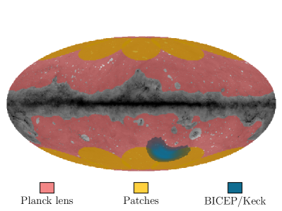
Figure 4: The light red regions denote the Planck lensing mask, used for computing the “full sky” average of GNILC CIB and $\phi^{\prime}$ map cross-correlation. The yellow regions are the eight patches with similar size and unpolarized dust amplitudes as the Bicep/Keck patch. These patches used for measuring the mean and scatter of the CIB auto-spectra and CIB$\times\phi^{\prime}$, which are used as inputs to simulating CIB and filtering the CIB map. The overlaps between the yellow patches are small and apodization is applied when calculating the auto- and cross-spectra. The Bicep/Keck patch is shaded in blue. The background is the Planck dust intensity map.

In these patches, we compute the auto-spectra and cross-spectra using PolSpice chon04 . We show the correlations $\rho_{L}$, defined as $C_{L}^{\rm I\phi^{\prime}}/\sqrt{C_{L}^{\rm II}C_{L}^{\phi\phi}}$, for a few different regions of the sky in Fig. 5. Here $I$ denotes the CIB map, $\phi^{\prime}$ denotes the Planck lensing estimate, and $C_{L}^{\phi\phi}$ is the theory spectrum from the fiducial cosmology used in planck2015cosmoparam . Comparing the correlations of the CIB map and the lensing map in the selected patches with that from the full overlap between the two maps (labeled “Full Sky”), we observe that the correlations within the patches are higher than the correlation in the larger region that includes lower Galactic latitudes, and hence higher dust levels. The full-overlap region correlation is $\sim 62\%$ for $L$ between 150 and 550, whereas the mean correlation in the patches is $\sim 69\%$ over the same $L$ range. Fig. 5 also shows the cross-correlation in the Bicep/Keck patch, which appears to be consistent with the eight circular patches.

As a cross check, we compare within the Bicep/Keck patch the cross-spectrum of the GNILC CIB map and the Planck lensing map against the cross-spectrum of a CIB map produced by lenz19 and the Planck lensing map. This CIB map has been cleaned using neutral hydrogen (HI) as a Galactic foreground tracer, with an HI column density threshold of $2.5\times 10^{20}$  cm^-2. We find the lensing correlation in the two CIB maps to be consistent with each other, thus providing additional evidence that in the Bicep/Keck map region, the GNILC CIB map does not show the reduced correlation which is expected, and seen, in regions closer to the Galactic plane.

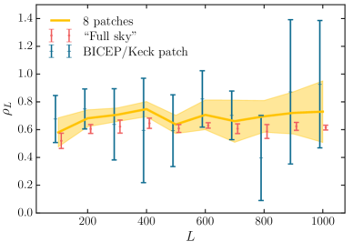
Figure 5: The binned correlation factor $\rho_{L}=C_{L}^{\rm I\phi^{\prime}}/\sqrt{C_{L}^{\rm II}C_{L}^{\phi\phi}}$ for the eight patches, the full sky, and the Bicep/Keck patch. “Full sky” corresponds to the overlap area between the Planck lensing mask and the GNILC CIB map. The $\rho_{L}$ in the Bicep/Keck patch is consistent with those measured across the eight patches. The yellow band denoted by “8 patches” is the mean and standard deviation of $\rho_{L}$ across the 8 patches. The error bars for the red and blue points are computed by taking the standard error of $\rho_{L}$ within each $\Delta L=100$ bin. The red and blue points are shifted for clarity.

The filter and normalization of the $\phi$ tracer is given in general form in Eq. 8. In this case, we take it as the average over the eight patches of the cross-spectra of the CIB and the lensing map divided by the average of the CIB auto-spectra:

$$\phi^{\rm CIB}_{LM}=\left(\frac{\langle C_{L}^{\rm I\phi^{\prime}}\rangle_{\rm patches}}{\langle C_{L}^{\rm II}\rangle_{\rm patches}}\right)I_{LM}.$$ (15)

To further prevent Galactic dust contamination, we additionally impose a $L_{\rm min}=100$ cut. This filter and normalization is applied to the real data as well as the simulated CIB realizations which are described in the next section. We render the normalized and Wiener filtered CIB $a_{\ell m}$ and its associated gradients to Healpix maps of $N_{\rm side}=512$, and then interpolate and convert the gradient maps to derivatives with respect to our pixel grid. The derivatives are shown in the middle panels of Fig. 3.

III.2.2 CIB simulations

We use CIB simulations to estimate the expected level of lensing $B$-modes in the lensing template, to form the bandpower covariance in the likelihood analysis, and as inputs to null tests.

We generate CIB simulations based on the input Gaussian $\phi$ fields of the Bicep/Keck simulation set described in Sec. III.1.2. To convert the $\phi$ fields to CIB fields, we use the auto-spectrum of the CIB, $C_{L}^{\rm II}$, and the cross-spectrum of the CIB and the Planck lensing estimate $\phi^{\prime}$, $C_{L}^{\text{I}\phi^{\prime}}$. We construct each CIB field by rescaling each input $\phi$ field so that the cross-spectrum of the rescaled field with the input $\phi$ is $C_{L}^{\text{I}\phi^{\prime}}$. We then add to the rescaled $\phi$ field Gaussian noise so that its auto-spectrum is $C_{L}^{\rm II}$. Formally, we construct the signal part of the CIB simulations, $I_{LM}^{S}$, as

$$I_{LM}^{S}=\frac{C_{L}^{\rm I\phi^{\prime}}}{C_{L}^{\phi\phi}}\phi_{LM}$$ (16)

where $\phi_{LM}$ are the spherical harmonic coefficients of the input $\phi$ fields. We construct the noise part of the CIB simulations, $I_{LM}^{N}$, by generating Gaussian random fields with power spectrum described by $C_{L}^{\rm II}$$-$ ($C_{L}^{\text{I}\phi^{\prime}}$)${}^{2}/C_{L}^{\phi\phi}$. The total CIB field is the sum of the two terms $I_{LM}=I_{LM}^{S}+I_{LM}^{N}$.

We have 499 realizations of $\phi_{LM}$. For each $\phi_{LM}$, we form $I_{LM}$ as described in the previous paragraph with $C_{L}^{\phi\phi}$ from the input theory and $C_{L}^{\rm II}$ and $C_{L}^{\text{I}\phi^{\prime}}$ sampled from the measured mean and covariance of $C_{L}^{\rm II}$ and $C_{L}^{\text{I}\phi^{\prime}}$ from the 8 patches selected in Sec. III.2.1. In the limit of many realizations, the simulated $I_{LM}$ will have the same covariance structure in $C_{L}^{\rm II}$ and $C_{L}^{\text{I}\phi^{\prime}}$ as measured from the 8 patches. The advantage of sampling $C_{L}^{\rm II}$ and $C_{L}^{\text{I}\phi^{\prime}}$ as opposed to using the measured mean from the 8 patches is that the potential patch-to-patch variation of the CIB auto-spectrum, and the cross-spectrum between CIB and $\phi^{\prime}$, is built into the simulations. Therefore, the uncertainties in the CIB measurements are propagated to the uncertainty in the $r$ measurement.

At this point we use the method described in Sec. II.1 to undeflect the combined $Q/U$ data and simulation maps with the data and simulation CIB maps to form the real and simulated lensing templates. The lensing templates from the real data are shown in the bottom panels of Fig. 3.

We have now laid out the lensing template construction, the extension of the Bicep/Keck analysis framework, and the input simulations and data used in this paper. The next steps include demonstrating the robustness of these extensions to potential biases and misestimations of inputs.

IV Pipeline and Simulation Validation

In this section, we demonstrate the robustness of the pipeline in the limit of perfect delensing, quantify the level of bias to our inference of $r$ given potential misestimations in the inputs to our simulations, and estimate the impact on $\sigma(r)$ given variations in the simulation setup. To do that we use the set of lensed-$\Lambda$CDM+dust+noise simulations ($r=0$) from the BK14 paper. We run maximum-likelihood searches of the baseline lensed-$\Lambda$CDM+dust+synchrotron+$r$ model as described in Appendix E.3 of the BK14 paper, in this case adding a lensing template.

IV.1 $r$ recovery with perfect delensing

To validate the addition of the lensing template as a pseudo-band in the Bicep/Keck analysis framework, we run maximum-likelihood searches in two configurations—unlensed input CMB skies without lensing templates, and lensed input CMB skies with perfect lensing templates. The perfect lensing templates are constructed by differencing the filtered, noiseless, lensed and unlensed $Q/U$ skies. If the likelihood works as intended, we expect the recovered $r$ values from the two sets of simulations to be extremely close to each other on a realization-by-realization basis. We find that the differences between the recovered $r$ values $|\Delta r|\lesssim 0.002$. We also find that at our current noise level, even if we have perfect knowledge of the lensing $B$-modes in our patch, the uncertainty on $r$ is reduced only by 26% from $\sigma(r)=0.024$ to $\sigma(r)=0.018$. This means that lensing uncertainty is subdominant compared to uncertainties from foregrounds and instrument noise in the BK14 data set.

IV.2 Biases to $r$ from misestimations of inputs

We investigate the bias to $r$ from the following: (1) misestimation of the correlation between the CIB map and $\phi$, and (2) biases in polarization efficiency in the input $Q/U$ maps.

Misestimation of $C_{L}^{\text{I}\phi}$ : As discussed in Sec. III.2.1, we compute $C_{L}^{\rm II}$ and $C_{L}^{\text{I}\phi^{\prime}}$ used in the normalization and Wiener filter of the CIB map as the mean of the $C_{L}^{\rm II}$ and $C_{L}^{\text{I}\phi^{\prime}}$ from 8 patches. In addition, we generate simulations of CIB based on the mean and scatter of the $C_{L}^{\rm II}$ and $C_{L}^{\text{I}\phi^{\prime}}$ spectra measured from the patches. Here, we consider the case in which the actual CIB cross-spectrum with $\phi$ is offset from the measured mean $C_{L}^{\text{I}\phi^{\prime}}$. A plausible way in which the measured $C_{L}^{\text{I}\phi^{\prime}}$ might be biased from the true $C_{L}^{\text{I}\phi}$ is through a bias in the $\phi^{\prime}$ reconstruction due to CIB in the input temperature maps. In that case, the measured $C_{L}^{\text{I}\phi^{\prime}}$ would contain a term that comes from CIB$\times\phi({\rm CIB,CIB})$, where $\phi({\rm CIB,CIB})$ denotes the CIB power that is leaked through the $\phi$ estimator applied to the CMB maps.

We construct a test for this bias, which proceeds as follows: using the measured mean $C_{L}^{\rm II}$ and $C_{L}^{\text{I}\phi^{\prime}}$, we generate simulated CIB skies as described in Sec. III.2.2. This set of simulations is the assumed truth. We then generate 2 sets of CIB skies whose $C_{L}^{\text{I}\phi^{\prime}}$ is either half a $\sigma_{\rm sp}$ above or below the measured mean $C_{L}^{\text{I}\phi^{\prime}}$, where $\sigma_{\rm sp}$ is measured from the spread across the 8 patches. We process these CIB skies as if they had the mean $C_{L}^{\text{I}\phi^{\prime}}$, i.e. we normalize and Wiener filter these maps using the mean $C_{L}^{\text{I}\phi^{\prime}}$ and $C_{L}^{\rm II}$. We then proceed to construct lensing templates and calculate auto- and cross-spectra with the rest of the BK14 maps, exactly as in the baseline analysis. The bandpower covariance matrix is derived using lensing templates constructed from the nominal, unbiased set of CIB skies. We then run maximum-likelihood searches on these two sets of simulations for the model parameters $r$, $A_{\mathrm{d}}$, $A_{\mathrm{sync}}$, $\beta_{\mathrm{d}}$, and $\beta_{\mathrm{s}}$. We determine the bias on $r$ by comparing the means of the maximum likelihood $r$ values from the nominal set and the half-$\sigma_{\rm sp}$ offset sets. We observe that the mean $r$ is biased by 0.2$\sigma$, where $\sigma$ denotes the uncertainty of the $r$ measurement (i.e. the width of the $r$ distribution of the nominal set).

To get a sense of how relevant this bias is, we compare the half-$\sigma_{\rm sp}$ offset we introduce into the simulations to a worst-case scenario of CIB leakage in the reconstructed $\phi^{\prime}$ map. Reference omori17 estimated the term CIB$\times\phi({\rm CIB,CIB})$ using $\phi^{\prime}$ reconstructed from the Planck 545 GHz maps without foreground cleaning and found the bias to be below $\sim$5% for $L<1024$, the $L$ range used in this work. A 5% bias is smaller than the half $\sigma_{\rm sp}$ shift considered. Furthermore, the Planck lensing map used to calculate $C_{L}^{\text{I}\phi^{\prime}}$ was constructed using the SMICA input maps that are foreground-suppressed. Therefore, we expect the 0.2$\sigma$ bias to be an overestimate of potential biases from misestimating $C_{L}^{\text{I}\phi^{\prime}}$.

Misestimation of polarization efficiency: The Planck collaboration has found that their polarization efficiency calibration could potentially be biased at the 1–2% level (see e.g. Table 9 of planck2018III, ). The SPTpol $Q/U$ maps are calibrated using a Planck $E$-mode map henning18 . Therefore, it is reasonable to ask by how much $r$ would be biased if the calibration of the input $Q/U$ maps is biased.

We construct the test by artificially scaling the SPTpol $Q/U$ simulated maps low by 1.7% and analyzing the maps as if they had the original amplitudes. In other words, similar to the half-$\sigma_{\rm sp}$ $C_{L}^{\text{I}\phi^{\prime}}$ shift test above, the rest of the pipeline is held identical and the only change is the input SPTpol $Q/U$ maps. For simplicity, instead of using the combined $Q/U$ map, we use only SPTpol simulated maps for this test. Comparing the mean of the recovered maximum likelihood $r$ values for the nominal set with that for the biased set, we find negligible differences. We conclude that biases at this level in the polarization efficiency are not an issue for this analysis.

IV.3 Impact on $\sigma(r)$ from variations of inputs

We investigate the impact on $\sigma(r)$ from two effects: (1) non-Gaussianities in the input CIB map, and (2) inclusion of patch-to-patch variation in $C_{L}^{\rm II}$ and $C_{L}^{\text{I}\phi^{\prime}}$in the generation of the CIB realizations.

Non-Gaussianity of the CIB: As discussed in Sec. III.2.2, we generate our CIB simulations based on the $\phi$ realizations used to lens the simulated CMB input skies. While the $\phi$ realizations are Gaussian, the true $\phi$ has some non-Gaussianities due to non-linear growth of structure boehm16 . However, the contribution to lensing $B$-modes from non-Gaussian $\phi$ is subdominant over the angular scales considered lewis2016 . It is thus sufficient to model $\phi$ and the portion of CIB that correlates with $\phi$, the signal term (Eq. 16), as Gaussian. In addition to the signal term, we simulate the noise term of the CIB $I_{LM}^{N}$—the portion of the CIB that does not correlate with $\phi$—as Gaussian realizations given the measured $C_{L}^{\rm II}$, $C_{L}^{\text{I}\phi^{\prime}}$, and the input $C_{L}^{\phi\phi}$. However, the CIB is known to be quite non-Gaussian; its bispectra at the angular scales relevant to this work have been measured by planck2013XXX with high signal-to-noise. Therefore, one could imagine that simulating the CIB $I_{LM}^{N}$ as Gaussian fluctuations would cause the lensing template fluctuation to be underestimated. With the underestimation of the lensing template fluctuation, $\sigma(r)$ would be underestimated. Here we estimate the impact on $\sigma(r)$ when we increase the lensing template fluctuation.

To get a handle on how much to increase the lensing template fluctuation, we build lensing templates using a simulated CIB sky from Websky mocks, which are built based on an approximation to full N-body halo catalogs stein18 ; stein20 . From the full-sky CIB realization, we make 80 cutouts of size similar to the Bicep/Keck patch, undeflect-and-difference the $Q/U$ maps, and compute the lensing template bandpower variances. We then generate matching Gaussian realizations of CIB using the $C_{L}^{\rm II}$ and $C_{L}^{\text{I}\phi}$ measured between the simulated CIB map and the corresponding $\phi$ map (provided as a $\kappa$ map, where $\kappa=-\nabla^{2}\phi/2$). Using these Gaussian CIB realizations, we generate lensing templates and calculate their bandpower variances. For the $L$ range considered in this analysis, the ratio of the lensing template 1$\sigma$ uncertainties between templates generated from Gaussian CIB and those from N-body based CIB is 0.97 $\pm$ 0.07. This suggests that the lensing template bandpower variance is sufficiently modeled using Gaussian simulations. Furthermore, namikawa19 performed a similar test using galaxy densities as $\phi$ tracer and found that the difference in the lensing template covariance between the Gaussian and their simulations is within the Monte-Carlo uncertainty of the number of simulations considered.

Since the above tests could still be limited by the number of non-Gaussian simulated CIB skies, we ask how much $\sigma(r)$ could be impacted because of some low level of unmodeled non-Gaussianity in the $\phi$ tracer. To do that, we increase the values in the lensing template auto-spectrum sub-block of the bandpower covariance matrix by 10% and perform maximum-likelihood searches on the baseline set of simulations. The resultant $\sigma(r)$ estimated from the width of the $r$ value distribution is negligibly different to the baseline case. Therefore, we conclude that at the current level of noise, unmodeled non-Gaussianities of the CIB have negligible impact on the uncertainty of the $r$ measurement.

Patch-to-patch variation in $C_{L}^{\rm II}$ and $C_{L}^{\text{I}\phi^{\prime}}$: We construct the CIB realizations using samples of $C_{L}^{\rm II}$ and $C_{L}^{\text{I}\phi^{\prime}}$ drawn from the measured covariance of $C_{L}^{\rm II}$ and $C_{L}^{\text{I}\phi^{\prime}}$ across 8 patches. By doing this we incorporate the patch-to-patch variation in the CIB auto- and cross-spectrum with $\phi^{\prime}$ into the uncertainty on $r$. Here we check how large this effect is by comparing the $\sigma(r)$ estimated from a set of CIB simulations generated with fixed $C_{L}^{\rm II}$ and $C_{L}^{\text{I}\phi^{\prime}}$ with that estimated from a set of CIB simulations generated from a distribution of $C_{L}^{\rm II}$ and $C_{L}^{\text{I}\phi^{\prime}}$. We find that the $\sigma(r)$ from these two sets of simulations are compatible to within MC uncertainty. This means that the uncertainty on $r$ introduced by the uncertainties in $C_{L}^{\rm II}$ and $C_{L}^{\text{I}\phi^{\prime}}$ is subdominant compared with the noise and sample variance of the lensing templates.

Having estimated the biases to $r$ caused by possible biases in the CIB and $Q/U$ maps and found them to be small, and having shown the impact on $\sigma(r)$ due to unmodeled non-Gaussianity of the CIB to be minimal, we now turn to testing the robustness of the simulations against unmodeled Galactic foregrounds using the data themselves.

V Systematics checks

Previous Bicep/Keck papers include “jackknife” internal consistency tests on the 95 and 150 GHz maps used here bk1 ; bk5 ; bk6 . In this section, we provide similar tests of the auto- and cross-spectra of the newly introduced lensing template. We consider the following ways in which the simulations can fail to sufficiently describe the statistics of the lensing template:

1. Galactic dust in the input 150 GHz $Q/U$ maps leaks into the lensing template,

2. low-$\ell$ systematic residuals in the Planck polarization maps leak into the lensing template,

3. non-Gaussian Galactic dust residuals in the CIB map introduce extra power in the lensing template beyond that described by Gaussian modeling of uncorrelated power.

All of the above would (i) increase the power of the lensing template auto-spectrum, and (ii) introduce potential chance coupling with the observed $B$-modes.

Galactic dust power is sub-dominant to $E$-mode power over the angular scales relevant to producing the lensing $B$-mode template, and the simulated $Q/U$ maps used in Sec. III.1.2 do not include a dust component. However, we would still like to check that the Galactic dust component in the $Q/U$ data maps does not significantly contribute to the lensing template auto-spectrum. For the CIB map, any components that contribute to the CIB auto-spectrum but are uncorrelated with $\phi^{\prime}$ are modeled as Gaussian fluctuations. Therefore, the unmodeled non-Gaussian Galactic foregrounds could contribute extra fluctuation in the lensing templates when used to undeflect the CMB maps. In addition, they could contribute extra template power when deflecting the unmodeled Galactic foregrounds in the $Q/U$ maps.

To address the question of whether the simulations are a sufficient description of the data given these unmodeled effects, we test the consistency of the lensing template auto- and cross-spectra against simulations. Specifically, we perform spectrum-difference tests where we compare the difference spectrum of data between the baseline $\ell$ & $L$ ranges and variant $\ell$ & $L$ ranges against the corresponding differences in simulation. We calculate two quantities, $\chi^{2}$ and $\chi$, as follows. Firstly

$$\chi^{2}_{\rm sys}=\Delta C_{\ell}^{\dagger}\,{\rm Cov^{-1}}\Delta C_{\ell},$$ (17)

where $\Delta C_{\ell}$ denotes the binned data difference spectrum and ${\rm Cov}$ is the bandpower covariance matrix formed from the difference spectra of the corresponding simulations. And secondly

$$\chi_{\rm sys}=\sum_{\ell}\Delta C_{\ell}/\sigma_{\ell,\rm diff},$$ (18)

where $\sigma_{\ell,\rm diff}$ denotes the standard deviation from the simulation difference spectra. Fig. 6 shows the difference spectra for the lensing template auto-spectrum (LT$\times$LT), lensing template cross-spectrum with the BK14 95 GHz map (LT$\times$BK14₉₅), and lensing template cross-spectrum with the BK14 150 GHz map (LT$\times$BK14₁₅₀). The PTE values from $\chi^{2}_{\rm sys}$ and $\chi_{\rm sys}$ are listed in Table 1.

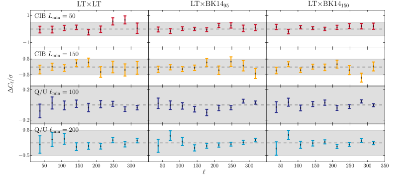
Figure 6: Difference bandpowers ($\Delta C_{\ell}$, see definition in text) between the baseline analysis and analyses with one parameter changed, and the uncertainties on those difference bandpowers, both scaled by the statistical uncertainties on the baseline analysis bandpowers. The label at the top left hand corner of each row indicates which parameter has been modified and how it is modified. The left to right columns show the difference bandpowers from the lensing template auto-spectrum, lensing template cross-spectrum with the BK14 95 GHz map, and lensing template cross-spectrum with the BK14 150 GHz map. The gray bands indicate the 0.5$\sigma$ statistical uncertainty of the baseline spectra. The $\chi_{\rm sys}^{2}$ and PTE of the difference bandpowers are listed in Table 1. We find the data difference bandpowers to be consistent with the spread in the simulation difference bandpowers.

Table 1: The PTE values from $\chi^{2}_{\rm sys}$ and $\chi_{\rm sys}$ (separated by a comma) with different CIB input $L_{\rm min}$ and $Q/U$ map input $\ell_{\rm min}$, compared with the baseline setup. LT$\times$LT , LT$\times$95, and LT$\times$150 denote the lensing template auto-spectrum, lensing template cross-spectrum with the BK14 95 GHz map, and with the BK14 150 GHz map, respectively.

Variation / spectrum	LT$\times$LT	LT$\times$95	LT$\times$150
CIB $L_{\rm min}$ = 50	0.36, 0.12	0.80, 0.23	0.66, 0.09
CIB $L_{\rm min}$ = 150	0.91, 0.67	0.68, 0.63	0.25, 0.88
$Q/U$ $\ell_{\rm min}$ = 100	0.76, 0.70	0.09, 0.84	0.34, 0.52
$Q/U$ $\ell_{\rm min}$ = 200	0.76, 0.75	0.36, 0.57	0.28, 0.62

V.1 $L$-cuts on CIB map

At large angular scales the CIB map could be contaminated by Galactic dust and thus a test in which the $L_{\rm min}$ for the CIB map is varied could be sensitive to its impact. The unmodeled non-Gaussianity of residual Galactic foregrounds in the CIB map would cause the lensing template to have larger variance than it would otherwise. We test the hypothesis that the simulations are sufficient descriptions of the real data by differencing the lensing template auto- and cross-spectra generated using the baseline $L_{\rm min}=100$ for the CIB map and those generated with $L_{\rm min}=50$ and $L_{\rm min}=150$. The PTEs from the $L_{\rm min}$ difference spectra show that the data differences are sufficiently described by the simulation-difference distributions.

V.2 $\ell$-cuts on $Q/U$ maps

Galactic dust contributes a fraction of the total power in the $Q/U$ maps on the largest scales. Additionally, there could be low levels of unmodeled systematic residuals planck2016SRoll in the Planck $Q/U$ maps that could leak power to the lensing templates. Similar to the test done with the CIB map, we set the $\ell_{\rm min}$ of the input $Q/U$ map to two different levels compared to the baseline (no explicit $\ell_{\rm min}$ set) and compute difference spectra between the variant $\ell_{\rm min}$ and the baseline. For $\ell_{\rm min}=100$ and $\ell_{\rm min}=200$, we find the PTEs from the difference spectra to be consistent with the simulation-difference distributions.

We thus conclude that at the current level of noise, the lensing template auto-spectrum and the cross-spectra with the 95 GHz and 150 GHz maps do not contain unmodeled systematics from large angular scales of the input $Q/U$ and CIB maps large enough to be incompatible with the simulation distributions.

VI Results

We now proceed to repeat the parameter constraint analysis from the BK14 paper bk6 including the lensing template extension described and validated above. We present two main results in this work. First, we estimate $\sigma(r)$ with delensing by running maximum-likelihood searches on the set of lensed-$\Lambda$CDM+dust+noise simulations from BK14. Second, we explore the likelihood space of the real data and provide constraints on $r$ and the foreground model parameters.

In Sec. III, we described the construction of a lensing template using the Planck GNILC CIB map and the combined $Q/U$ maps from SPTpol, Bicep/Keck, and Planck. Fig. 7 shows the auto- and cross-spectra of this lensing template with the maps that most significantly constrain the model parameters—the Bicep/Keck 95 & 150 GHz maps, and the Planck 353 GHz map. The lensing template auto- and cross-spectra shown in Fig. 7, plus the additional cross-spectra with the other bands of WMAP and Planck, are the new additions to the bandpower data vector input to the likelihood analysis. It is interesting to note that the error bars are much smaller at low $\ell$ for LT$\times$LT than for LT$\times$150. This is because, although the 150 GHz map noise is very small, the dust sample variance is large.

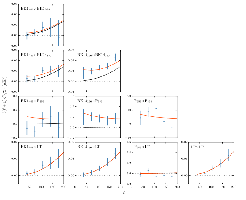
Figure 7: $BB$ auto- and cross-spectra calculated using Bicep2/Keck 95 & 150 GHz maps, the Planck 353 GHz map, and the lensing template developed in this paper. The black lines show the model expectation values for lensed-$\Lambda$CDM, while the red lines show the expectation values of the baseline lensed-$\Lambda$CDM+dust model from the BK14 analysis ($r=0$, $A_{\mathrm{d}}=4.3$ $\mu{\mathrm{K}^{2}}$, $\beta_{\mathrm{d}}=1.6$, $\alpha_{\mathrm{d}}=-0.4$), and the error bars are scaled to that model. Compared to the BK14 $BB$ spectra, which contain both foregrounds and lensing components, the lensing template represents an alternate way to estimate the lensing $B$-modes which is largely foreground-immune, and, as we see here, provides good signal-to-noise in the resulting auto- and cross-spectra.

VI.1 Reduction in $\sigma(r)$

The inclusion of the lensing template cross-spectra reduces the effective sample variance of the lensing component of the observed $B$-modes. This is the reason that the uncertainty of the $r$ component can be reduced when we add a lensing template to the likelihood.

In BK14, we introduced $\sigma(r)$ as a measure of the intrinsic constraining power of a given set of experimental data. In contrast to the width of the 68% highest posterior density interval as derived from the real data this measure is not subject to noise fluctuation within that single realization. To compare the $\sigma(r)$ from the BK14 data set and the BK14 data set with lensing template included, we repeat the analysis of Appendix E.3 of the BK14 paper. We run maximum-likelihood searches with the baseline lensed-$\Lambda$CDM+dust+synchrotron+$r$ model on the lensed-$\Lambda$CDM+dust+noise simulations for the two cases. The parameters and priors are the same as in BK14 and are summarized in Table 2. The amplitudes at $\ell=80$ of the dust and synchrotron $BB$ spectra defined at 353 GHz and 23 GHz are denoted by $A_{\mathrm{d}}$ and $A_{\mathrm{sync}}$, respectively; $\beta$ and $\alpha$ denote the frequency and spatial spectral indices, with subscripts $d$ and $s$ referring to dust and synchrotron respectively; $\epsilon$ denotes the dust-synchrotron correlation. Flat priors are applied to $r$, $A_{\mathrm{d}}$, $A_{\mathrm{sync}}$ & $\alpha_{\mathrm{d}}$, and Gaussian priors are applied to $\beta_{\mathrm{d}}$ & $\beta_{\mathrm{s}}$. Fig. 8 shows the distributions of maximum likelihood $r$, $A_{\mathrm{d}}$, and $A_{\mathrm{sync}}$ values. With the inclusion of the lensing template, we reduce $\sigma(r)$ from $0.024$ to $0.022$, a $\sim 10\%$ reduction.

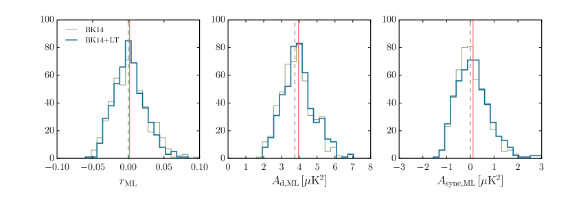
Figure 8: Histograms of maximum-likelihood values of $r$, $A_{\mathrm{d}}$, and $A_{\mathrm{sync}}$ from 499 realizations of BK14+LT (blue) and BK14 (gray) lensed-$\Lambda$CDM+dust+noise simulations in the baseline model with 6 free parameters: $r$, $A_{\mathrm{d}}$, $A_{\mathrm{sync}}$, $\beta_{\mathrm{d}}$, $\beta_{\mathrm{s}}$ and $\alpha_{\mathrm{d}}$. The red lines mark the means of the distributions for the BK14+LT simulation set and the gray dashed lines mark the input values. $\sigma(r)$ from the BK14+LT (BK14) simulation set is $0.022$ ($0.024$) from the leftmost panel.

Table 2: Priors imposed on each parameter for both maximum-likelihood search and posterior sampling for the baseline analysis. $\mathcal{U}(a,b)$ denotes uniform distribution between $[a,b]$. $\mathcal{N}(\mu,\sigma^{2})$ denotes normal distribution with mean $\mu$ and variance $\sigma^{2}$.

Parameter	ML search	Sampling
$r$	$\mathcal{U}(-0.5,0.5)$	$\mathcal{U}(0,0.5)$
$A_{\mathrm{d}}$	$\mathcal{U}(-2,15)$	$\mathcal{U}(0,15)$
$A_{\mathrm{sync}}$	$\mathcal{U}(-2,15)$	$\mathcal{U}(0,50)$
$\beta_{\mathrm{d}}$	$\mathcal{N}(1.6,0.11^{2})$	$\mathcal{N}(1.59,0.11^{2})$
$\beta_{\mathrm{s}}$	$\mathcal{N}(-3.1,0.3^{2})$	$\mathcal{N}(-3.1,0.3^{2})$
$\alpha_{\mathrm{d}}$	$\mathcal{U}(-1,0)$	$\mathcal{U}(-1,0)$
$\alpha_{\mathrm{s}}$	fixed	$\mathcal{U}(-1,0)$
$\epsilon$	fixed	$\mathcal{U}(0,1)$

We also generate simulated lensing templates using only one of SPTpol, Bicep/Keck, and Planck for the input $Q/U$ maps. We add the single-experiment lensing template to the BK14 simulation set and perform maximum-likelihood searches. We find that the $\sigma(r)$ from LT_SPTpol, LT_BICEP/Keck, and LT_Planck to be 0.0223, 0.0230, and 0.0236 respectively. This shows that the SPTpol $Q/U$ maps contribute most to recovering the lensing $B$-modes. The fact that LT_BICEP/Keck contributes more than LT_Planck shows that the signal-to-noise per mode at low $\ell$ is more important than having a wider range in $\ell$ for the particular combination of the $\ell$ range and noise levels between Bicep/Keck and Planck.

VI.2 Parameter posteriors of BK14 with delensing

We now repeat the eight-parameter likelihood evaluation of the real data as in the BK14 paper. We again use COSMOMC (cosmomc, ) and the lensed-$\Lambda$CDM+dust+synchrotron+$r$ model with parameters and priors summarized in Table 2. Fig. 9 shows the posterior distributions of the baseline analysis compared with the BK14 result. The peak and 68% credible regions of the marginalized $r$ distribution are shifted down from the BK14 values of $0.028^{+0.026}_{-0.025}$ to $0.027^{+0.023}_{-0.022}$ when the lensing template is included. The 95% C.L. upper limit on $r_{0.05}$ is reduced from $0.090$  to $0.082$. Some of the other constraints are $A_{\mathrm{d}}=4.2^{+1.1}_{-0.9}$ $\mu{\mathrm{K}^{2}}$ and $A_{\mathrm{sync}}<3.7$ $\mu{\mathrm{K}^{2}}$ (95% C.L.). The maximum-likelihood model (including priors) in the 8D parameter space is: $r_{0.05}=0.025$, $A_{\mathrm{d}}=4.0$ $\mu{\mathrm{K}^{2}}$, $A_{\mathrm{sync}}=1.4$ $\mu{\mathrm{K}^{2}}$, $\beta_{\mathrm{d}}=1.6$, $\beta_{\mathrm{s}}=-3.1$, $\alpha_{\mathrm{d}}=-0.17$, $\alpha_{\mathrm{s}}=-0.95$, and $\epsilon=0.00$. Against this model, we compute $\chi^{2}=(d-m)^{\dagger}{\rm Cov^{-1}}(d-m)=768$ for the $9\times 78=702$ data bandpowers. We compare this number against the distribution in simulations finding a PTE of 0.15. We conclude that the model is a sufficient description of the data at present.

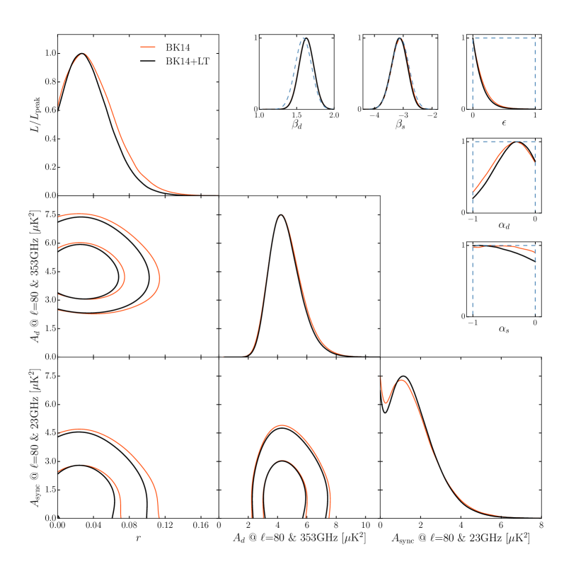
Figure 9: Posterior distributions of the baseline model parameters given the BK14+LT data set (black lines) compared with the BK14 data set (red lines, which are the same as the black lines in Fig. 4 of the BK14 paper). The lensing template is constructed using combined $Q/U$ maps from SPTpol, Bicep/Keck, and Planck (Sec. III.1.3) and a CIB map as the $\phi$ tracer (Sec. III.2.1). The 95% C.L. upper limit on the tensor-to-scalar ratio tightens from $r_{0.05}<0.090$ to $r_{0.05}<0.082$ with the addition of the lensing template. The parameters $A_{\mathrm{d}}$ and $A_{\mathrm{sync}}$ are the amplitudes of the dust and synchrotron B-mode spectra, where $\beta$ and $\alpha$ are the frequency and spatial spectral indices respectively. The dust-synchrotron correlation parameter is denoted by $\epsilon$. The up-turn of the 1D posterior distribution of $A_{\mathrm{sync}}$ as it approaches zero comes from the increased volume allowed by the $\epsilon$ parameter as $\epsilon$ becomes ambiguous when $A_{\mathrm{sync}}=0$. In the 1D panels for the $\alpha$, $\beta$, and $\epsilon$ parameters, the blue dashed lines denote the priors for each parameter.

We perform a couple of variations to the baseline analysis to explore degeneracies amongst model parameters that are important to lensing, and changes in $r$ with different input data sets. In the baseline analysis, the lensing $BB$ spectrum is taken as the $\Lambda$CDM expectation in both normalization and shape. As an alternative we re-scale this spectrum by the parameter $A_{\rm L}$ and sample the posterior distribution in the $\Lambda$CDM+$A_{\rm L}$ model space. Secondly, as is done in Sec. VI.1, we form input lensing templates using $Q/U$ maps from one of the three experiments instead of combining them. We discuss the results of each variation in the following paragraphs.

When we allow $A_{\rm L}$ to float, we note a $A_{\rm L}-r$ degeneracy in the BK14 data set, as shown in Fig. 10, and as was previously noted in an earlier Bicep/Keck analysis bkp . When the lensing template is added to the BK14 data set, the degeneracy between $r$ and $A_{\rm L}$ is reduced. In this model space, the peak and 68% credible regions of the marginalized $r$ distribution with and without the lensing template are $0.025^{+0.023}_{-0.022}$ and $0.009^{+0.031}_{-0.009}$, and the upper limits on $r$ are $r_{0.05}<0.081$ and $r_{0.05}<0.079$ respectively. The peak and 68% credible regions of $A_{\rm L}$ with and without the lensing template are $1.03\pm 0.10$ and $1.21\pm 0.17$ respectively. The shift in the peak $A_{\rm L}$ is consistent with expectations from simulations, where 25% of the simulation realizations have $A_{\rm L}$ shifts with absolute magnitude larger than that seen in data. We see that with the addition of the lensing template, we are able to better constrain the lensing power in the measured auto- and cross-spectra across the different frequencies and thereby reduce the probability of mis-assigning power to lensing.

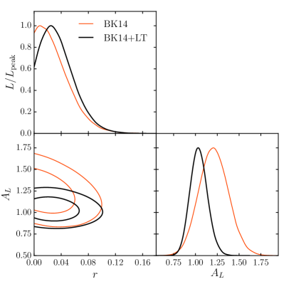
Figure 10: Posterior distributions on $r$ and $A_{\rm L}$, a parameter used to scale the lensing $BB$ power, from an alternative analysis in which the amplitude of lensing is a free parameter. With the addition of the lensing template, the probability of shuffling lensing power to other parameters is reduced, thus the degeneracy between $r$ and $A_{\rm L}$ is reduced.

We show in Fig. 11 the $r$ posterior distributions from analyses in the lensed-$\Lambda$CDM model space using lensing templates constructed from $Q/U$ maps coming from only one of the three experiments, SPTpol, Bicep/Keck and Planck. We see that the peaks of the $r$ posteriors from the Bicep/Keck-only and the Planck-only cases are close to the baseline case, while the width of the $r$ posterior from the Planck-only case is a bit larger than the baseline case. The larger $r$ posterior uncertainty is expected given the larger $\sigma(r)$ from the Planck-only simulation set in Sec. VI.1. The peak of the $r$ posterior for the SPTpol-only case is shifted up slightly compared with the baseline case. This might seem slightly surprising given that the SPTpol $Q/U$ maps contribute most of the weight in the combined $Q/U$ maps over a broad range of angular scales. To quantify the probability of the observed shift between the baseline case and the SPTpol-only case, we extract the best-fit $r$ values from the baseline simulation set and the SPTpol-only lensing template simulation set. Restricting to the subset with positive best-fit $r$ in the baseline setup, we count the fraction of realizations that have larger best-fit $r$ differences between the SPTpol-only and the baseline set than is seen in the data. We find 20% of the simulations fit this criterion and thus we conclude that what is observed in the data is typical of the expected fluctuations.

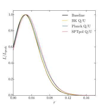
Figure 11: The $r$ posterior curves from the baseline analysis, along with $r$ curves from analyses using lensing templates constructed from $Q/U$ maps from only one of the three experiments: Bicep/Keck, Planck, and SPTpol. The shifts in the curves are consistent with expectations from simulations.

VII Conclusion

In this work, we build on the Bicep/Keck analysis framework and demonstrate, for the first time, improvements to constraints on the tensor-to-scalar ratio $r$ with delensing. With the addition of a lensing template, we reduce the uncertainty of the $r$ estimate by constraining the lensing $B$-mode contribution to the observed $B$-modes. We construct the lensing template using an undeflect-and-difference approach, in which we undeflect the observed $Q/U$ maps by a $\phi$ tracer, and then difference the undeflected maps from the input maps. The $Q/U$ maps we use are a 150 GHz combination of SPTpol observations from 2013–2015, Bicep/Keck observations up to 2014, and the Planck satellite full-mission observations. The $\phi$ tracer we use is a CIB map constructed using the GNILC algorithm from Planck data. The resulting lensing template is added as a pseudo-frequency band to the BK14 dataset, in which Bicep/Keck  WMAP  and Planck maps are used to constrain Galactic foregrounds and $r$.

We present two key results from this analysis. First, we estimate $\sigma(r)$ using our lensed-$\Lambda$CDM+dust+noise simulation set. We find maximum likelihood values of the baseline model parameters for each simulation realization and take the mean and standard deviation over the 499 realizations. We find that, with the addition of the lensing template, $\sigma(r)$ improves from $0.024$ in BK14 to $0.022$, a $\sim 10\%$ improvement. The second main result is the posterior peak value, 68% credible region, and upper limit on $r$ when we add the lensing template to the BK14 data set. With delensing, the peak and 68% credible regions shift from $r=0.028^{+0.026}_{-0.025}$ to $r=0.027^{+0.023}_{-0.022}$, and the 95% C.L. upper limit on $r$ is reduced from $0.090$ to $0.082$.

We estimate the impact on $r$ from potential biases in the inputs used to construct the simulated lensing templates. We find the biases to $r$ from misestimating the cross-spectrum of the CIB and $\phi$ to be small, and the biases to $r$ from biases in polarization efficiency of the CMB $Q/U$ maps to be negligible. We find negligible difference in $\sigma(r)$ due to modeling the non-Gaussian CIB field as Gaussian for this data set, and that the uncertainties in the CIB auto-spectrum and the CIB$\times\phi$ cross-spectrum contribute sub-dominantly to $\sigma(r)$. We perform checks against potential unmodeled systematic contaminations to the lensing template. This includes Galactic foregrounds leaking into the lensing template through either the input $Q/U$ maps or the input CIB map. We show that the data lensing template is sufficiently well-described by the simulations. Therefore we conclude that the results are robust against these sources of systematics given the current noise levels.

At the BK14 level of map noise and Galactic foreground variance, simulations indicate that perfect delensing would reduce $\sigma(r)$ from $0.024$ to $0.018$. This implies that the variance from lensing $B$-modes is not the dominant source of uncertainty ($<30\%$) when constraining $r$ in this data set. However, with current and upcoming ground-based CMB telescopes, e.g. Bicep Array biceparray20 , SPT-3G bender18 , AdvACT, Simons Array, Simons Observatory SO18 , and CMB-S4 cmbs4-sb1 , the millimeter-wave sky will be mapped with ever higher signal-to-noise. Lensing $B$-modes will become a dominant source of uncertainty, and delensing will be crucial to break the floor of $\sigma(r)$ set by the lensing variance. For example, while in the most recent Bicep/Keck $r$ analysis BK15 bk10 lensing variance continues to be subdominant, in the upcoming result BK18 lensing variance contributes roughly half of the $r$ uncertainty budget. Projecting further, without delensing, the Bicep Array experiment $\sigma(r)$ would plateau at $\sim$0.006. However, this $\sigma(r)$ could be reduced by a factor of about 2.5 with delensing using a $\phi$ field reconstructed using CMB maps from the SPT-3G experiment. This is a much more significant reduction in the uncertainty on $r$ than is achieved in this work.

To reach the target $\sigma(r)$ of $5\times 10^{-4}$ for the next-generation ground-based CMB experiment CMB-S4, more than 90% of the lensing sample variance needs to be removed s4pgw . Delensing to such low residual levels requires high values of $\rho_{L}$, the correlation between the $\phi$ tracer and the underlying $\phi$ field. In addition to using $\phi$ maps reconstructed from low-noise, high-resolution CMB observations (e.g. wu2019, ; pblens2019, ; actlens, ), higher $\rho_{L}$ tracers could be obtained by combining different tracers (e.g. manzotti18, ; yu17, ) and using optimal methods (e.g. seljakhirata04, ; lensit, ; bayeslens, ; caldeira, ). We will be exploring various approaches to delensing (e.g. bayeslens, ) in future joint analyses of Bicep/Keck and SPT-3G data, confronting delensing algorithms with real-world non-idealities and developing techniques to mitigate systematics, readying our analysis for the future of low-noise data and the possibility of detecting PGWs.

Appendix A Lensing template construction methods

In this paper, we have used a map-space “undeflect-and-difference” method to construct the lensing template. Previous works have inferred the lensing $B$-modes $\hat{B}^{\mathrm{lens}}(\boldsymbol{\ell})$ by lensing the observed $E$-modes to first order in $\phi$ given a $\phi$ tracer. Specifically,

$$\hat{B}^{\mathrm{lens}}(\boldsymbol{\ell})=\int\frac{d^{2}\boldsymbol{\ell}^{\prime}}{(2\pi)^{2}}W(\boldsymbol{\ell},\boldsymbol{\ell}^{\prime})\bar{\phi}(\boldsymbol{\ell}-\boldsymbol{\ell}^{\prime})\bar{E}(\boldsymbol{\ell}^{\prime})\,,$$ (19)

where $W(\boldsymbol{\ell},\boldsymbol{\ell}^{\prime})=\boldsymbol{\ell}^{\prime}\cdot(\boldsymbol{\ell}-\boldsymbol{\ell}^{\prime})\sin(2\varphi_{\boldsymbol{\ell},\boldsymbol{\ell}^{\prime}})$, and $\bar{E}$ and $\bar{\phi}$ are the Wiener filtered $E$-modes and $\phi$ tracer respectively (e.g. manzotti17, ). An advantage to this formulation is that by acting on the $E$-modes of the observed sky only, noise in the lensing template is reduced versus the undeflect-and-difference method. This extra noise enters by undeflecting $Q/U$ maps which also contain $B$-modes. While the signal contribution from the $B$-modes is small, the level of noise fluctuations is similar to those in the $E$-modes, which contribute noise to the undeflect-and-difference templates. However, this is not a fundamental limitation to the map-space approach as implemented in this paper. One could Fourier transform the $Q/U$ maps to $E/B$-modes, null the $B$-modes, and then transform back to $Q/U$ maps before performing the undeflect-and-difference operation, which would remove this specific noise. In fact, we experimented with adding these steps and found that for the present case, the reduction in lensing template noise is fractionally very small for $\ell<500$.

For future analyses, we will revisit the algorithm used to produce the lensing template to further improve its signal-to-noise. Besides removing the extra noise contribution, other possible improvements include filling in the region outside the SPTpol coverage (as seen in Fig. 2) using the information available from Bicep/Keck and Planck.

- (1) M. Kamionkowski and E. D. Kovetz, “The Quest for B Modes from Inflationary Gravitational Waves,” ARA&A 54 (Sept., 2016) 227–269, arXiv:1510.06042 [astro-ph.CO].
- (2) Planck Collaboration, Y. Akrami, F. Arroja, et al., “Planck 2018 results. X. Constraints on inflation,” arXiv e-prints (July, 2018) arXiv:1807.06211, arXiv:1807.06211 [astro-ph.CO].
- (3) U. Seljak and M. Zaldarriaga, “Signature of Gravity Waves in the Polarization of the Microwave Background,” Phys. Rev. Lett. 78 no. 11, (Mar., 1997) 2054–2057, arXiv:astro-ph/9609169 [astro-ph].
- (4) M. Kamionkowski, A. Kosowsky, and A. Stebbins, “A Probe of Primordial Gravity Waves and Vorticity,” Phys. Rev. Lett. 78 no. 11, (Mar., 1997) 2058–2061, arXiv:astro-ph/9609132 [astro-ph].
- (5) Planck Collaboration, R. Adam, P. A. R. Ade, et al., “Planck intermediate results. XXX. The angular power spectrum of polarized dust emission at intermediate and high Galactic latitudes,” Astr. & Astroph. 586 (Feb., 2016) A133, arXiv:1409.5738 [astro-ph.CO].
- (6) N. Krachmalnicoff, E. Carretti, C. Baccigalupi, et al., “S-PASS view of polarized Galactic synchrotron at 2.3 GHz as a contaminant to CMB observations,” Astr. & Astroph. 618 (Oct., 2018) A166, arXiv:1802.01145 [astro-ph.GA].
- (7) A. Lewis and A. Challinor, “Weak gravitational lensing of the CMB,” Phys. Rep. 429 (June, 2006) 1–65, astro-ph/0601594.
- (8) D. Hanson, S. Hoover, A. Crites, et al., “Detection of B-Mode Polarization in the Cosmic Microwave Background with Data from the South Pole Telescope,” Phys. Rev. Lett. 111 no. 14, (Oct., 2013) 141301, arXiv:1307.5830 [astro-ph.CO].
- (9) Polarbear Collaboration, P. A. R. Ade, Y. Akiba, et al., “A Measurement of the Cosmic Microwave Background B-mode Polarization Power Spectrum at Sub-degree Scales with POLARBEAR,” Astrophys. J. 794 (Oct., 2014) 171, arXiv:1403.2369.
- (10) R. Keisler, S. Hoover, N. Harrington, et al., “Measurements of Sub-degree B-mode Polarization in the Cosmic Microwave Background from 100 Square Degrees of SPTpol Data,” Astrophys. J. 807 (July, 2015) 151.
- (11) T. Louis, E. Grace, M. Hasselfield, et al., “The Atacama Cosmology Telescope: two-season ACTPol spectra and parameters,” JCAP 6 (June, 2017) 031, arXiv:1610.02360.
- (12) BICEP2 Collaboration, Keck Array Collaboration, P. A. R. Ade, et al., “Improved Constraints on Cosmology and Foregrounds from BICEP2 and Keck Array Cosmic Microwave Background Data with Inclusion of 95 GHz Band,” Physical Review Letters 116 no. 3, (Jan., 2016) 031302, arXiv:1510.09217.
- (13) POLARBEAR Collaboration, P. A. R. Ade, M. Aguilar, et al., “A Measurement of the Cosmic Microwave Background B-mode Polarization Power Spectrum at Subdegree Scales from Two Years of polarbear Data,” Astrophys. J. 848 (Oct., 2017) 121, arXiv:1705.02907.
- (14) BICEP2 Collaboration, Keck Array Collaboration, P. A. R. Ade, et al., “Constraints on Primordial Gravitational Waves Using Planck, WMAP, and New BICEP2/Keck Observations through the 2015 Season,” Phys. Rev. Lett. 121 no. 22, (Nov, 2018) 221301, arXiv:1810.05216 [astro-ph.CO].
- (15) BICEP2/Keck Collaboration, Planck Collaboration, P. A. R. Ade, et al., “Joint Analysis of BICEP2/Keck Array and Planck Data,” Phys. Rev. Lett. 114 no. 10, (Mar., 2015) 101301, arXiv:1502.00612 [astro-ph.CO].
- (16) A. Manzotti, K. T. Story, W. L. K. Wu, et al., “CMB Polarization B-mode Delensing with SPTpol and Herschel,” Astrophys. J. 846 (Sept., 2017) 45, arXiv:1701.04396.
- (17) J. Carron, A. Lewis, and A. Challinor, “Internal delensing of Planck CMB temperature and polarization,” JCAP 5 (May, 2017) 035, arXiv:1701.01712.
- (18) Planck Collaboration, N. Aghanim, Y. Akrami, et al., “Planck 2018 results. VIII. Gravitational lensing,” arXiv e-prints (Jul, 2018) arXiv:1807.06210, arXiv:1807.06210 [astro-ph.CO].
- (19) S. Adachi, M. A. O. Aguilar Faúndez, Y. Akiba, et al., “Internal delensing of cosmic microwave background polarization B-modes with the POLARBEAR experiment,” arXiv e-prints (Sep, 2019) arXiv:1909.13832, arXiv:1909.13832 [astro-ph.CO].
- (20) D. Han, N. Sehgal, A. MacInnis, et al., “The Atacama Cosmology Telescope: Delensed Power Spectra and Parameters,” arXiv e-prints (July, 2020) arXiv:2007.14405, arXiv:2007.14405 [astro-ph.CO].
- (21) W. Hu and T. Okamoto, “Mass Reconstruction with Cosmic Microwave Background Polarization,” Astrophys. J. 574 no. 2, (Aug., 2002) 566–574, arXiv:astro-ph/0111606 [astro-ph].
- (22) G. Simard, D. Hanson, and G. Holder, “Prospects for Delensing the Cosmic Microwave Background for Studying Inflation,” Astrophys. J. 807 no. 2, (Jul, 2015) 166, arXiv:1410.0691 [astro-ph.CO].
- (23) B. D. Sherwin and M. Schmittfull, “Delensing the CMB with the cosmic infrared background,” Phys. Rev. D 92 no. 4, (Aug., 2015) 043005, arXiv:1502.05356 [astro-ph.CO].
- (24) W. L. K. Wu, L. M. Mocanu, P. A. R. Ade, et al., “A Measurement of the Cosmic Microwave Background Lensing Potential and Power Spectrum from 500 deg2 of SPTpol Temperature and Polarization Data,” Astrophys. J. 884 no. 1, (Oct., 2019) 70, arXiv:1905.05777 [astro-ph.CO].
- (25) Planck Collaboration, N. Aghanim, M. Ashdown, et al., “Planck intermediate results. XLVIII. Disentangling Galactic dust emission and cosmic infrared background anisotropies,” Astr. & Astroph. 596 (Dec., 2016) A109, arXiv:1605.09387 [astro-ph.CO].
- (26) Planck Collaboration, P. A. R. Ade, N. Aghanim, et al., “Planck 2015 results. XV. Gravitational lensing,” Astr. & Astroph. 594 (Sept., 2016) A15, arXiv:1502.01591.
- (27) W. Hu, “Weak lensing of the CMB: A harmonic approach,” Phys. Rev. D 62 (Aug., 2000) .
- (28) E. Anderes, B. D. Wandelt, and G. Lavaux, “Bayesian Inference of CMB Gravitational Lensing,” Astrophys. J. 808 no. 2, (Aug., 2015) 152, arXiv:1412.4079 [astro-ph.CO].
- (29) D. Green, J. Meyers, and A. van Engelen, “CMB delensing beyond the B modes,” JCAP 12 (Dec., 2017) 005, arXiv:1609.08143.
- (30) BICEP2 Collaboration, P. A. R. Ade, R. W. Aikin, et al., “Detection of B-Mode Polarization at Degree Angular Scales by BICEP2,” Physical Review Letters 112 no. 24, (June, 2014) 241101, arXiv:1403.3985.
- (31) S. Hamimeche and A. Lewis, “Likelihood analysis of CMB temperature and polarization power spectra,” Phys. Rev. D 77 no. 10, (May, 2008) 103013, arXiv:0801.0554.
- (32) J. E. Austermann, K. A. Aird, J. A. Beall, et al., “SPTpol: an instrument for CMB polarization measurements with the South Pole Telescope,” in Millimeter, Submillimeter, and Far-Infrared Detectors and Instrumentation for Astronomy VI, vol. 8452 of Proc. SPIE, p. 84521E. Sept., 2012. arXiv:1210.4970 [astro-ph.IM].
- (33) J. E. Carlstrom, P. A. R. Ade, K. A. Aird, et al., “The 10 Meter South Pole Telescope,” PASP 123 (May, 2011) 568, arXiv:0907.4445 [astro-ph.IM].
- (34) J. W. Henning, J. T. Sayre, C. L. Reichardt, et al., “Measurements of the Temperature and E-mode Polarization of the CMB from 500 Square Degrees of SPTpol Data,” Astrophys. J. 852 (Jan., 2018) 97, arXiv:1707.09353.
- (35) K. M. Smith, D. Hanson, M. LoVerde, C. M. Hirata, and O. Zahn, “Delensing CMB polarization with external datasets,” JCAP 2012 no. 6, (June, 2012) 014, arXiv:1010.0048 [astro-ph.CO].
- (36) D. Lenz, O. Doré, and G. Lagache, “Large-scale Maps of the Cosmic Infrared Background from Planck,” Astrophys. J. 883 no. 1, (Sep, 2019) 75, arXiv:1905.00426 [astro-ph.CO].
- (37) Planck Collaboration, N. Aghanim, M. Ashdown, et al., “Planck intermediate results. XLVIII. Disentangling Galactic dust emission and cosmic infrared background anisotropies,” Astr. & Astroph. 596 (Dec., 2016) .
- (38) M. Remazeilles, J. Delabrouille, and J.-F. Cardoso, “Foreground component separation with generalized Internal Linear Combination,” Mon. Not. Roy. Astron. Soc. 418 (Nov., 2011) 467–476, arXiv:1103.1166.
- (39) A. Maniyar, G. Lagache, M. Béthermin, and S. Ilić, “Constraining cosmology with the cosmic microwave and infrared backgrounds correlation,” Astr. & Astroph. 621 (Jan, 2019) A32, arXiv:1809.04551 [astro-ph.CO].
- (40) G. Chon, A. Challinor, S. Prunet, E. Hivon, and I. Szapudi, “Fast estimation of polarization power spectra using correlation functions,” Mon. Not. Roy. Astron. Soc. 350 no. 3, (May, 2004) 914–926, arXiv:astro-ph/0303414 [astro-ph].
- (41) Planck Collaboration, P. A. R. Ade, N. Aghanim, et al., “Planck 2015 results. XIII. Cosmological parameters,” Astr. & Astroph. 594 (Sept., 2016) A13, arXiv:1502.01589 [astro-ph.CO].
- (42) Y. Omori, R. Chown, G. Simard, et al., “A 2500 deg2 CMB Lensing Map from Combined South Pole Telescope and Planck Data,” Astrophys. J. 849 no. 2, (Nov, 2017) 124, arXiv:1705.00743 [astro-ph.CO].
- (43) Planck Collaboration, N. Aghanim, Y. Akrami, et al., “Planck 2018 results. III. High Frequency Instrument data processing and frequency maps,” arXiv e-prints (Jul, 2018) arXiv:1807.06207, arXiv:1807.06207 [astro-ph.CO].
- (44) V. Böhm, M. Schmittfull, and B. D. Sherwin, “Bias to CMB lensing measurements from the bispectrum of large-scale structure,” Phys. Rev. D 94 no. 4, (Aug, 2016) 043519, arXiv:1605.01392 [astro-ph.CO].
- (45) A. Lewis and G. Pratten, “Effect of lensing non-Gaussianity on the CMB power spectra,” JCAP 2016 no. 12, (Dec., 2016) 003, arXiv:1608.01263 [astro-ph.CO].
- (46) Planck Collaboration, P. A. R. Ade, N. Aghanim, et al., “Planck 2013 results. XXX. Cosmic infrared background measurements and implications for star formation,” Astr. & Astroph. 571 (Nov, 2014) A30, arXiv:1309.0382 [astro-ph.CO].
- (47) G. Stein, M. A. Alvarez, and J. R. Bond, “The mass-Peak Patch algorithm for fast generation of deep all-sky dark matter halo catalogues and its N-body validation,” Mon. Not. Roy. Astron. Soc. 483 no. 2, (Feb, 2019) 2236–2250, arXiv:1810.07727 [astro-ph.CO].
- (48) G. Stein, M. A. Alvarez, J. R. Bond, A. van Engelen, and N. Battaglia, “The Websky Extragalactic CMB Simulations,” arXiv e-prints (Jan., 2020) arXiv:2001.08787, arXiv:2001.08787 [astro-ph.CO].
- (49) T. Namikawa and R. Takahashi, “Impact of nonlinear growth of the large-scale structure on CMB B -mode delensing,” Phys. Rev. D 99 no. 2, (Jan, 2019) 023530, arXiv:1810.03346 [astro-ph.CO].
- (50) BICEP2 and Keck Array Collaborations, P. A. R. Ade, Z. Ahmed, et al., “BICEP2/Keck Array V: Measurements of B-mode Polarization at Degree Angular Scales and 150 GHz by the Keck Array,” Astrophys. J. 811 no. 2, (Oct., 2015) 126, arXiv:1502.00643 [astro-ph.CO].
- (51) Planck Collaboration, N. Aghanim, M. Ashdown, et al., “Planck intermediate results. XLVI. Reduction of large-scale systematic effects in HFI polarization maps and estimation of the reionization optical depth,” Astr. & Astroph. 596 (Dec, 2016) A107, arXiv:1605.02985 [astro-ph.CO].
- (52) A. Lewis and S. Bridle, “Cosmological parameters from CMB and other data: a Monte- Carlo approach,” Phys. Rev. D66 (2002) 103511, astro-ph/0205436.
- (53) A. Schillaci, P. A. R. Ade, Z. Ahmed, et al., “Design and performance of the first BICEP Array receiver,” arXiv e-prints (Feb., 2020) arXiv:2002.05228, arXiv:2002.05228 [astro-ph.IM].
- (54) A. N. Bender, P. A. R. Ade, Z. Ahmed, et al., “Year two instrument status of the SPT-3G cosmic microwave background receiver,” in Millimeter, Submillimeter, and Far-Infrared Detectors and Instrumentation for Astronomy IX, vol. 10708 of Society of Photo-Optical Instrumentation Engineers (SPIE) Conference Series, p. 1070803. Jul, 2018. arXiv:1809.00036 [astro-ph.IM].
- (55) The Simons Observatory Collaboration, P. Ade, J. Aguirre, et al., “The Simons Observatory: Science goals and forecasts,” ArXiv e-prints (Aug., 2018) , arXiv:1808.07445.
- (56) CMB-S4 Collaboration, K. N. Abazajian, P. Adshead, et al., “CMB-S4 Science Book, First Edition,” ArXiv e-prints (Oct., 2016) , arXiv:1610.02743.
- (57) The CMB-S4 Collaboration, K. Abazajian, G. E. Addison, et al., “CMB-S4: Forecasting Constraints on Primordial Gravitational Waves,” arXiv e-prints (Aug., 2020) arXiv:2008.12619, arXiv:2008.12619 [astro-ph.CO].
- (58) M. A. Faúndez, K. Arnold, C. Baccigalupi, et al., “Measurement of the Cosmic Microwave Background Polarization Lensing Power Spectrum from Two Years of POLARBEAR Data,” Astrophys. J. 893 no. 1, (Apr., 2020) 85, arXiv:1911.10980 [astro-ph.CO].
- (59) B. D. Sherwin, A. van Engelen, N. Sehgal, et al., “Two-season Atacama Cosmology Telescope polarimeter lensing power spectrum,” Phys. Rev. D 95 no. 12, (June, 2017) 123529, arXiv:1611.09753 [astro-ph.CO].
- (60) A. Manzotti, “Future cosmic microwave background delensing with galaxy surveys,” Phys. Rev. D 97 no. 4, (Feb., 2018) 043527, arXiv:1710.11038 [astro-ph.CO].
- (61) B. Yu, J. C. Hill, and B. D. Sherwin, “Multitracer CMB delensing maps from Planck and WISE data,” Phys. Rev. D 96 no. 12, (Dec., 2017) 123511, arXiv:1705.02332 [astro-ph.CO].
- (62) U. Seljak and C. M. Hirata, “Gravitational lensing as a contaminant of the gravity wave signal in the CMB,” Phys. Rev. D 69 no. 4, (Feb., 2004) 043005, arXiv:astro-ph/0310163 [astro-ph].
- (63) J. Carron and A. Lewis, “Maximum a posteriori CMB lensing reconstruction,” Phys. Rev. D 96 no. 6, (Sept., 2017) 063510, arXiv:1704.08230 [astro-ph.CO].
- (64) M. Millea, E. Anderes, and B. D. Wandelt, “Bayesian delensing delight: sampling-based inference of the primordial CMB and gravitational lensing,” arXiv e-prints (Feb., 2020) arXiv:2002.00965, arXiv:2002.00965 [astro-ph.CO].
- (65) J. Caldeira, W. L. K. Wu, B. Nord, et al., “DeepCMB: Lensing reconstruction of the cosmic microwave background with deep neural networks,” Astronomy and Computing 28 (July, 2019) 100307, arXiv:1810.01483 [astro-ph.CO].
- (66) F. Pérez and B. E. Granger, “IPython: a system for interactive scientific computing,” Computing in Science and Engineering 9 no. 3, (May, 2007) 21–29. https://ipython.org.
- (67) J. D. Hunter, “Matplotlib: A 2d graphics environment,” Computing in Science & Engineering 9 no. 3, (2007) 90–95.
- (68) P. Virtanen, R. Gommers, T. E. Oliphant, et al., “SciPy 1.0: Fundamental Algorithms for Scientific Computing in Python,” Nature Methods 17 (2020) 261–272.
- (69) A. Zonca, L. Singer, D. Lenz, et al., “healpy: equal area pixelization and spherical harmonics transforms for data on the sphere in python,” Journal of Open Source Software 4 no. 35, (Mar., 2019) 1298. https://doi.org/10.21105/joss.01298.
- (70) K. M. Górski, E. Hivon, A. J. Banday, et al., “HEALPix: A Framework for High-Resolution Discretization and Fast Analysis of Data Distributed on the Sphere,” Astrophys. J. 622 (Apr., 2005) 759–771, arXiv:astro-ph/0409513.