Comparison of explicit and mean-field models of cytoskeletal filaments with crosslinking motors

Abstract

In cells, cytoskeletal filament networks are responsible for cell movement, growth, and division. Filaments in the cytoskeleton are driven and organized by crosslinking molecular motors. In reconstituted cytoskeletal systems, motor activity is responsible for far-from-equilibrium phenomena such as active stress, self-organized flow, and spontaneous nematic defect generation. How microscopic interactions between motors and filaments lead to larger-scale dynamics remains incompletely understood. To build from motor-filament interactions to predict bulk behavior of cytoskeletal systems, more computationally efficient techniques for modeling motor-filament interactions are needed. Here we derive a coarse-graining hierarchy of explicit and continuum models for crosslinking motors that bind to and walk on filament pairs. We compare the steady-state motor distribution and motor-induced filament motion for the different models and analyze their computational cost. All three models agree well in the limit of fast motor binding kinetics. Evolving a truncated moment expansion of motor density speeds the computation by $10^{3}$–$10^{6}$ compared to the explicit or continuous-density simulations, suggesting an approach for more efficient simulation of large networks. These tools facilitate further study of motor-filament networks on micrometer to millimeter length scales.

1 Introduction

The cytoskeleton generates force and reorganizes to perform important cellular processes [1], including cell motility [2, 3], cytokinesis [4], and chromosome segregation in mitosis [5]. The cytoskeleton is made of polymer filaments, molecular motors, and associated proteins. The two best-studied cytoskeletal filaments are actin and microtubules [1]. It remains incompletely understood how diverse cytoskeletal structures dynamically assemble and generate force of pN to nN [1, 2].

Force generation and reorganization in the cytoskeleton depend on the activity of crosslinking motor proteins that align and slide pairs of filaments (Figure 1). Reorganization of actin networks by myosin motors is important for muscle contraction [6, 7, 8], cell crawling and shape change [9, 10, 11], and cytokinesis [12, 4]. Microtubule sliding by crosslinking kinesin and dynein motors contributes to mitotic spindle assembly [13, 14, 15, 16, 5], chromosome segregation [17, 18, 19, 20], cytoplasmic stirring in Drosophila oocytes [21], and beating of cilia and flagella [22, 23, 24].

Filament-motor interactions produce diverse cellular structures and dynamics, but linking molecular properties of motors to larger-scale assembly behavior remains challenging. Crosslinking motors vary in binding affinity, speed, processivity, and force-velocity relation. These same ingredients can be reconstituted and show dynamic self-organization into asters or contractile bundles [25, 26, 27], active liquid crystals [28, 29, 30, 31], or other structures [32, 33, 34]. Even in reconstituted systems, our ability to predict and control dynamics and self-organization is limited.

Improved theory and simulation of cytoskeletal assemblies with crosslinking motors would allow better prediction of both cellular and reconstituted systems. Currently few mesoscale modeling methods for filament-motor systems are available between explicit particle simulations and continuum hydrodynamic theory. Explicit motor simulations have several existing software tools, including Cytosim [35], MEDYAN [36], and AFINES [37], and others [38]. Explicit motor simulations are straightforward to extend to include, for example, a new force-velocity relation or motor cooperativity. However, the cost of explicit particle simulations scales linearly or quadratically with the number of particles (depending on the type of interactions), making simulation of large systems challenging. Continuum models of coarse-grained fields can be computationally tractable and predict macroscopic behavior [39, 40, 41, 42, 43, 44, 45, 46]. Current continuum models invoke symmetry considerations to determine the structure of the model without reference to an underlying microscopic mechanisms [39, 47, 48, 49], or simplify a microscopic model by making assumptions about the physics of motor [50, 51, 52, 53, 54, 55, 43, 56, 57]. Furthermore, previous continuum theories have coarse-grained the filament distribution, with simplifying assumptions about the motor distribution. This presents an opportunity to better understand how the distribution of motors evolves and affects filament motion. Further development of mesoscale modeling techniques focusing on crosslinking motors could help bridge the gap between detailed explicit particle models and continuum theories.

To develop mesoscale modeling tools, we focus on the fundamental unit of a crosslinked filament network: two filaments with crosslinking motors that translate and rotate the filaments. We study three different model representations in a coarse-graining hierarchy and compare computational cost and accuracy. For explicit motors, we extend previous work that uses Brownian dynamics and kinetic Monte Carlo simulation to handle filament motion and binding kinetics [43, 56, 58, 59, 60, 61, 62]. At the first level of coarse-graining, we average over discrete bound motors to compute the continuum mean-field motor density (MFMD) between filaments, and evolve this density according to a first-order Fokker-Planck equation [58]. This requires computing the solution to a single partial differential equation (PDE) for each filament pair, rather than separately tracking each individual motor. The MFMD determines the force and torque on each filament needed to evolve its position and orientation. At the second level of coarse-graining, we expand the MFMD in moments to derive a system of ordinary differential equations (ODEs) for the time evolution of the moments. While the moment expansion does not close, an approximate treatment of filament motion can be modeled by low-order moments. To compare these three model implementations, we consider test cases of parallel, antiparallel, and perpendicular filaments. Under the same initial conditions, the three model implementations give similar results on average. Remarkably, the reduced moment expansion achieves a computational cost that is $10^{3}$–$10^{6}$ lower than the other models, suggesting a route to computationally tractable large-scale simulations.

2 Model overview

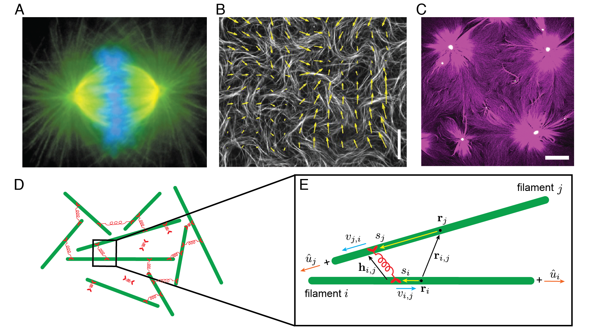
Figure 1: Experimental systems of cytoskeletal filaments with crosslinking motors and overview of the model. A-C Fluoresence microscopy images of cytoskeletal networks. A Mitotic spindle showing microtubules (green), chromosomes (blue), and spindle-pole component TPX2 (red) [63]. B Reconstituted active gel of microtubules (white) driven by crosslinking kinesin motor clusters with local flow field shown (yellow arrows) [28]. Scale bar: 80 $\mu$m. C Reconstituted active network of actin (magenta) and myosin-II (green) [64]. Scale bar: 50 $\mu$m. D Schematic of filament-motor network with green filaments and red motors. E Schematic of filament pair (green) crosslinked by a motor (red) with model variables position of filament $i$’s center ${\bf r}_{i}$, orientation vector of filament $i$ ${\hat{u}}_{i}$, vector between filament centers ${\bf r}_{i,j}={\bf r}_{j}-{\bf r}_{i}$, vector between motor heads ${\bf h}_{i,j}$, motor tether extension $|h_{i,j}|$, and motor speed on filament $i$ while attached to filament $j$.

We consider a pair of rigid, inextensible filaments that move and reorient under the force and torque applied by crosslinking motors. Filaments move in three dimensions, experience viscous drag, and are constrained to prevent overlaps. Motors bind to and unbind from the filaments consistent with detailed balance in binding. Crosslinking motors walk with a force-dependent velocity toward filament plus ends and unbind when they reach the ends. We investigate models at three levels: an explicit motor model where motors are represented with a discrete density, a continuum mean-field motor density (MFMD) model, and a moment expansion model.

2.1 Filaments

We model filament motion using Brownian dynamics, balancing the force applied by motors against viscous drag and constraint forces. Because the force that induces Brownian motion is typically smaller than that due to motors, we neglect Brownian noise [65].

Filaments translate according to the force-balance equation

$$\dot{{\bf r}}_{i}={\bf{M}}_{i}\left(\sum_{n}{\bf F}_{n,i}\right),$$ (1)

where ${\bf r}_{i}$ is the center of filament $i$ with mobility matrix ${\bf M}_{i}$ acted on by forces ${\bf F}_{n,i}$. The mobility matrix for a perfectly rigid rod in a viscous medium is

$${\bf M}_{i}=\left(\left(\gamma_{\parallel,i}-\gamma_{\perp,i}\right){\hat{u}}_{i}{\hat{u}}_{i}+\gamma_{\perp,i}{\bf I}\right)^{-1},$$ (2)

where $\bf I$ is the identity matrix and $\gamma_{\parallel,i}$ and $\gamma_{\perp,i}$ are the parallel and perpendicular drag coefficients with respect to the filament orientation ${\hat{u}}_{i}$. Cytoskeletal filaments with length $L_{i}$ and diameter $D_{{\rm fil}}$ typically have a large aspect ratio $L_{i}/D_{{\rm fil}}\gg 1$, so we approximate the drag coefficients using slender body theory [66].

The torque-balance equation is

$$\dot{{\hat{u}}}_{i}=\frac{1}{\gamma_{\theta,i}}\left(\sum_{n}{\bf T}_{n,i}\right)\times{\hat{u}}_{i},$$ (3)

where ${\bf T}_{n,i}$ are the torques acting on filament $i$ and $\gamma_{\theta,i}$ is the rotational drag coefficient about the center of filament $i$.

The force and torque exerted by crosslinking motors depend on where motors are attached, the motor tether extension, and the relative position and orientation of filaments. Given the crosslinking motor distribution along the filaments $\psi_{i,j}(s_{i},s_{j})$, where $s_{i}$ is the bound motor head position on filament $i$, the total crosslinking force and torque exerted by filament $i$ on filament $j$ are

$${\bf F}_{i,j} = \int_{L_{i}}\int_{L_{j}}{\bf f}_{i,j}(s_{i},s_{j})\psi_{i,j}(s_{i},s_{j})ds_{i}ds_{j},$$ (4)

$${\bf T}_{i,j} = \int_{L_{i}}\int_{L_{j}}s_{j}{\hat{u}}_{j}\times{\bf f}_{i,j}(s_{i},s_{j})\psi_{i,j}(s_{i},s_{j})ds_{i}ds_{j}.$$ (5)

where ${\bf f}_{i,j}(s_{i},s_{j})$ is the force exerted on filament $j$ by the crosslinking motor attached at $s_{i}$ and $s_{j}$ (Figure 1E). For brevity, we use subscripts on variables such as ${\bf f}_{i,j}$ to indicate that these are functions of the relative position and orientation of filaments $i$ and $j$. Our three model implementations all models use equations (4) and (5) to compute the force and torque that evolve filament position and orientation but differ in how the computation of $\psi_{i,j}$.

We constrain the motion of filaments to prevent overlap, which avoids numerical instabilities introduced by a hard potential between filaments. To implement the constraint, we construct a vector ${\hat{u}}_{{\rm min}}$ that is perpendicular to both infinite carrier lines defined by ${\hat{u}}_{i}$ and ${\hat{u}}_{j}$ and parallel to the vector of closest approach between these lines. The vector ${\hat{u}}_{{\rm min}}$ is used to define two normal planes that confine the filaments, leading to the modified force and torque

$$\widetilde{{\bf F}}_{i,j} = {\bf F}_{i,j}-({\bf F}_{i,j}\cdot{\hat{u}}_{{\rm min}}){\hat{u}}_{{\rm min}}$$ (6)

$$\widetilde{{\bf T}}_{i,j} = ({\bf T}_{i,j}\cdot{\hat{u}}_{{\rm min}}){\hat{u}}_{{\rm min}}.$$ (7)

Note that for filaments lying in the same confining plane and $|\hat{u}_{i}\cdot\hat{u}_{j}|<1$, ${\hat{u}}_{{\rm min}}={\bf 0}$ and our constraints break down. However, if only the first condition is satisfied, i.e., (anti)parallel filaments, $\widetilde{{\bf T}}_{i,j}=0$ and $\widetilde{{\bf F}}_{i,j}$ is parallel to ${\hat{u}}_{i}$ and ${\hat{u}}_{j}$. After computing the force and torque, we numerically integrate equations (1) and (3) to update filament position and orientation.

2.2 Motors

In our model motors bind and unbind, crosslink between two filaments, exert force and torque when crosslinking, and walk with a force-dependent velocity. Typically motor proteins diffuse in solution until they are near a filament, then stochastically bind to that filament. Once one head binds, the other head can bind to a second filament, forming a crosslink, or the motor can unbind. Crosslinking motors can unbind to a state with one head bound, or can unbind completely from both filaments. We consider an infinite reservoir of unbound motor proteins. The diffusion of motors in solution is fast relative to the motion of filaments, so we assume the motor reservoir has uniform, constant concentration. We neglect steric interactions between motors. This approximation holds for filaments sparsely populated with motors and motors that do not cluster on filaments or in solution.

Motors crosslinking filaments have a potential energy $U_{i,j}(s_{i},s_{j})$ (Figure 1). The energy depends on the motor head separation vector ${\bf h}_{i,j}(s_{i},s_{j})={\bf r}_{j}+s_{j}{\hat{u}}_{j}-({\bf r}_{i}+s_{i}{\hat{u}}_{i})$ that gives the motor tether extension

$$h_{i,j}(s_{i},s_{j})=\sqrt{r_{i,j}^{2}+s_{j}^{2}+s_{i}^{2}+2{\bf r}_{i,j}\cdot(s_{j}{\hat{u}}_{j}-s_{i}{\hat{u}}_{i})-2s_{i}s_{j}({\hat{u}}_{i}\cdot{\hat{u}}_{j})},$$ (8)

where ${\bf r}_{i,j}={\bf r}_{j}-{\bf r}_{i}$ and $r_{i,j}^{2}={\bf r}_{i,j}\cdot{\bf r}_{i,j}$ (Figure 1E).

The bound motor heads walk with a speed $v_{i,j}$ that depends on the force component on the motor head parallel to the walking direction, ${\hat{u}}_{i}\cdot{\bf f}_{j,i}$ [67]. This projected force is used to determine the motor speed via the force-velocity relation, as discussed below. This model is based on processive microtubule motors such as kinesin and dynein, but a similar model has been used for myosin minifilaments [36, 37].

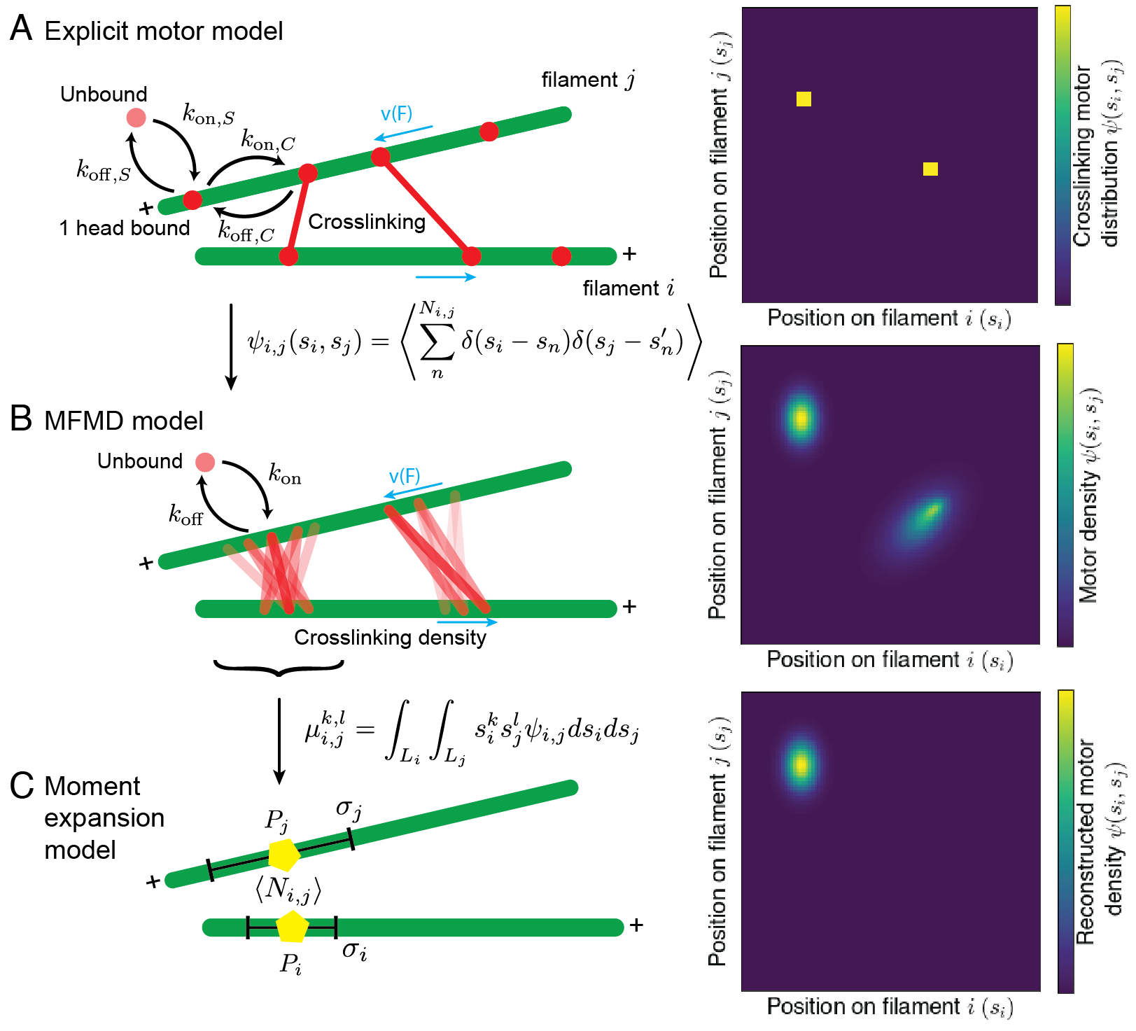
Figure 2: Comparison of motor representations in three hierarchical models with schematics on the left and 2D motor distributions on the right. A Explicit motor model with two-step binding kinetics. Unbound motors (light red circle) bind one head (red circle) to filaments and then crosslink (two red circles connected by red line). B Mean-field motor density model with motor distribution (translucent red bars). Average motor distribution moments $\mu_{i,j}^{k,l}$ with respect to powers of bound crosslink positions $s_{i}$ and $s_{j}$. Moments are related to bound motor number $N_{i,j}$ (pentagon color), mean motor head position $P_{i}$ (pentagon position), and standard deviation $\sigma_{i}$ (black lines). (right) 2D plot of reconstructed motor density using bivariate Gaussian approximation. For clarity, only moments derived from left-most crosslinking density distribution in (B) are used to reconstruct 2D motor distribution in (C.

3 Explicit motor model

In the explicit motor model individual bound motors are modeled, allowing fluctuations in bound motor number and binding kinetics that recover the correct equilibrium distribution of crosslinking proteins in the limit of no motor walking (Figure 2A) [43, 56, 59, 60, 61, 62].

3.1 Binding kinetics and stepping

A motor diffuses in solution until one of its heads bind to a filament; we model this by an infinite reservoir of unbound motors with a uniform and constant concentration $c_{o}$. Filaments have a linear binding site density $\epsilon$, and the binding site has an association constant $K_{a}$ (units of $\mu$M^-1). First motor head binding has rate

$$k_{{\rm on},S}=K_{a}c_{o}\epsilon L_{tot}k_{{\rm o},S},$$ (9)

where $L_{tot}=\sum_{i}L_{i}$ is the total length of filaments and $k_{{\rm o},S}$ is the bare (force-independent) unbinding rate for singly bound heads. All binding locations have equal binding probability. Singly bound motors unbind at rate $k_{{\rm off},S}=k_{{\rm o},S}$.

A motor with one head bound crosslink to another filament, which may stretch or compress its tether. This makes crosslinking kinetics force dependent; our models satisfy detailed balance in binding, so we recover the thermal equilibrium Boltzmann distribution in the limit of passive crosslinkers. Motor motion shifts the crosslinking distribution away from equilibrium. Motor unbinding rate can depend on the force applied to bound heads [68, 69, 70, 71, 72, 73]. Previous work shows how this force dependence can be included while maintaining detailed balance in binding [74, 75, 62]. For simplicity, here we include the force dependence in the binding rate only and discuss possible implications below. With one head bound to filament $i$ at position $s_{i}$, the free motor head binds to filament $j$ at position $s_{j}$ with a probability proportional to a Boltzmann factor of binding energy

$$P_{S\to C}\propto\exp(-\beta U_{i,j})$$ (10)

with $\beta=(k_{\textrm{B}}T)^{-1}$ (Figure 3A). Here $S\to C$ denotes the motor’s transition from a single head bound ($S$) to crosslinking ($C$). The total binding rate is computed by integration over all binding positions on filament $j$

$$k_{{\rm on},C}=\frac{\epsilon K_{\rm E}k_{{\rm o},C}}{V_{\rm bind}}\int_{L_{j}}e^{-\beta U_{i,j}}ds_{j},$$ (11)

where $k_{{\rm o},C}$ is the bare (force-independent) unbinding rate for a crosslinking motor, $K_{\rm E}$ is the crosslinking association constant. The unbound motor head explores a volume $V_{\rm bind}$ centered about the bound head, computed as the integral of the unbound head’s position weighted by the Boltzmann factor

$$V_{\rm bind}=\int e^{-\beta U_{i,j}}dr^{3}=4\pi\int_{0}^{R_{{\rm cut},C}}e^{-\beta U_{i,j}}r^{2}dr.$$ (12)

Beyond the cutoff radius $R_{{\rm cut},C}$ the integrand becomes small, enabling the use of a lookup table (Appendix B). The probability distribution of binding position depends on the Boltzmann factor. We recover the proper binding distribution through inverse transformation sampling of equation (11) (Appendix B.2).

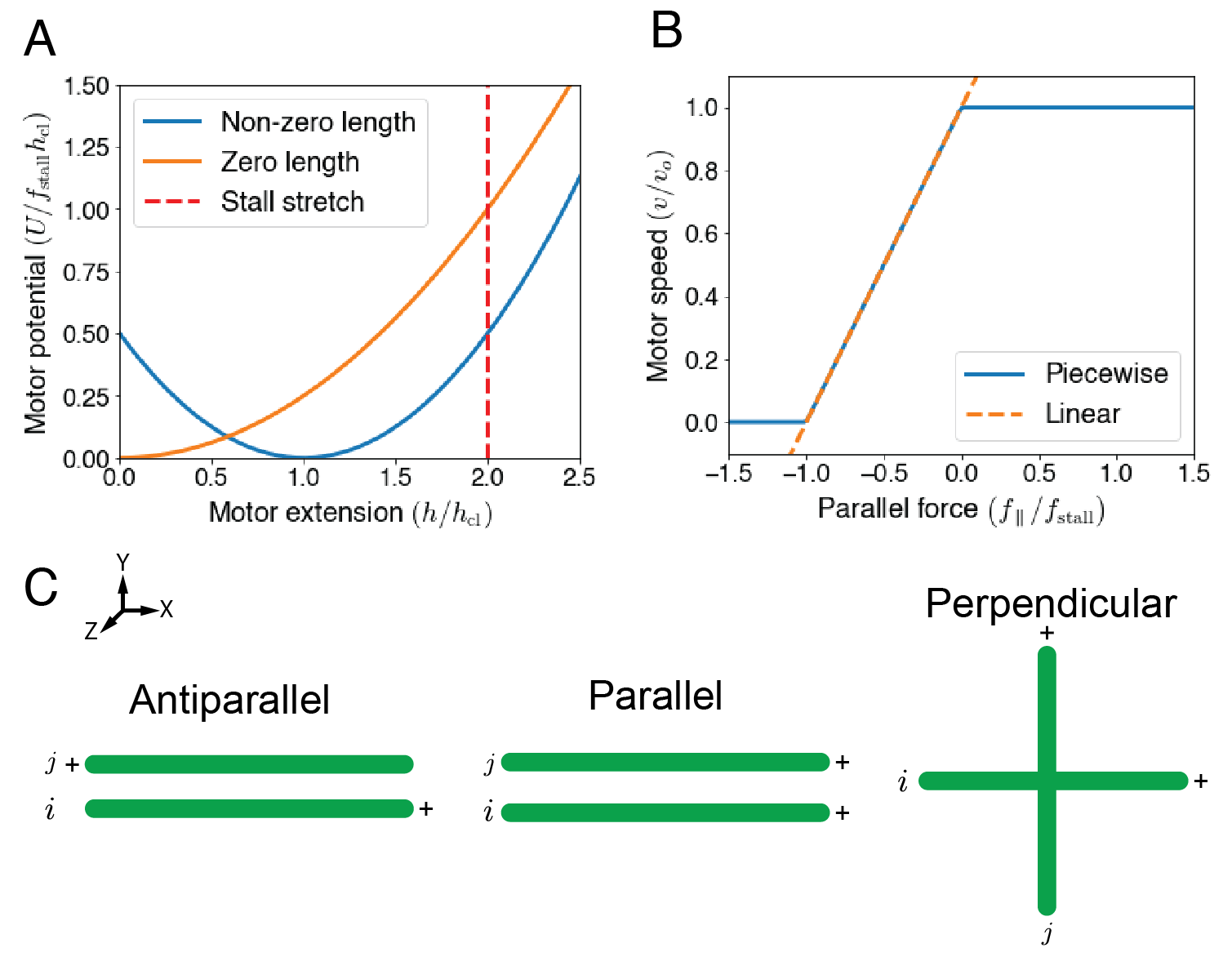
Figure 3: Choice for motor tether potential, force-velocity relation, and filament initial configurations. A Plot of the normalized potential energy in motor tether as a function of motor extension (blue) and equivalent zero-length tether potential (orange line). Both potentials have identical slope at the distance $f_{{\rm stall}}/k_{\rm cl}$ (red dashed line) where motors stall. B Plot of normalized motor speed as a function of force (blue) and its linear approximation (dashed orange). C Chosen initial configurations of pairs of 1$\mu m$ filaments. Filament centers are separated by $D_{\rm fil}$ = 25nm perpendicular to both filament orientation vectors.

As discussed above, the unbinding rate of a single head of a motor crosslinking two filaments is assumed to be force-independent,

$$k_{{\rm off},C}=k_{{\rm o},C}.$$ (13)

Force-dependent unbinding affects the density of motor proteins most when stretched[70]; larger motor stretch occurs when external force is applied against the force generated by motors. Therefore sliding filaments slowed only by drag, like those in active nematics, will be less affected by force-dependent unbinding than stationary filaments or jammed filaments like microtubules in mitotic spindles. We can include force-dependent unbinding in the explicit motor and MFMD model but not in the moment expansion model (Section 5). We chose the time step small enough that individual motors undergo only one transition per time step (Appendix A).

The motor force-velocity relation is

$$v_{i,j}=v({\hat{u}}_{i}\cdot{\bf f}_{j,i})=\begin{cases}v_{o},&0<{\hat{u}}_{i}\cdot{\bf f}_{j,i}\\ v_{o}\left(1+\frac{{\hat{u}}_{i}\cdot{\bf f}_{j,i}}{f_{{\rm stall}}}\right),&-f_{{\rm stall}}<{\hat{u}}_{i}\cdot{\bf f}_{j,i}<0\\ 0,&{\hat{u}}_{i}\cdot{\bf f}_{j,i}<-f_{{\rm stall}},\\ \end{cases}$$ (14)

where $f_{{\rm stall}}$ is the motor stall force (Figure 3B).

3.2 Distribution of explicitly modeled motors

The bound motor distribution is

$$\psi_{i,j}(s_{i},s_{j},t)=\sum_{n=1}^{N_{i,j}(t)}\delta(s_{i}-s_{n}(t))\delta(s_{j}-s^{\prime}_{n}(t)),$$ (15)

where $\delta(s_{i})$ is the Dirac delta function and $N_{i,j}$ is the total number of motors crosslinking filaments $i$ and $j$. Here $s_{n}$ and $s_{n}^{\prime}$ are the attached positions of the heads of the $n$th crosslinking motor. Motors with one head bound to filament $i$ have a distribution

$$\chi_{i}(s_{i},t)=\sum_{n=1}^{N_{i}(t)}\delta(s_{i}-s_{n}(t)),$$ (16)

where $N_{i}$ is the number of one-head bound motors on filament $i$. Only motors crosslinking exert forces between filament pairs, but $\chi_{i}$ and $\chi_{j}$ are needed to calculate the evolution of $\psi_{i,j}$.

4 Mean-field motor density model

Under typical experimental conditions, there can be tens to thousands of crosslinking motors between a filament pair. Motor force and torque fluctuations occur because of stochastic motor binding and unbinding. As the number of motors increases, the standard deviation relative to the mean decreases as $1/\sqrt{N}$. For our explicit motor model, antiparallel filaments with an average of 14 motors bound show a standard deviation in bound motor number of 27% of the mean. This shows that the fluctuations are quite significant for order 10 motors. The $1/\sqrt{N}$ scaling predicts that for an average of 1000 motors, the standard deviation would be only 3.2% of the mean. The force and torque scale similarly. Therefore, for large motor number, we may use the average motor distribution to derive a mean-field motor density (MFMD) to accurately describe force and torque on filaments by motors. We can then evolve the MFMD instead of explicit motors (Figure 2B). We previously showed that the average steady-state density of crosslinking motors between stationary parallel filaments agreed well with a solution to a multi-dimensional Fokker-Planck equation (FPE) [58]. Here, we expand this approach to model crosslinking motor density between filaments in three dimensions, allow filament motion, and study time-dependent behavior of coupled systems of motors and filaments.

For a one-step binding model, the MFMD evolves according to

$$\frac{\partial\psi_{i,j}(s_{i},s_{j},t)}{\partial t}=-\frac{\partial(v_{i,j}\psi_{i,j})}{\partial s_{i}}-\frac{\partial(v_{j,i}\psi_{i,j})}{\partial s_{j}}+k_{{\rm on}}-k_{{\rm off}}\psi_{i,j},$$ (17)

with motor velocity $v_{i,j}$, motor crosslinking rate $k_{{\rm on}}$, and unbinding rate $k_{{\rm off}}$. To satisfy detailed balance in binding, we use the rates $k_{{\rm on}}=2k_{{\rm o}}ce^{-\beta U_{i,j}(s_{i},s_{j})}$ and $k_{{\rm off}}=2k_{{\rm o}}$, with the effective concentration $c$ (units nm^-2) [58]. The factors of two occur because there are two ways a motor can crosslink. To numerically solve the hyperbolic equation (17), we use a first-order accurate upwind difference method (Appendix C).

The mean-field motor density model differs from the explicit model in that motors with one head bound are not modeled explicitly. To properly compare the different binding models, we establish a mapping of parameters between these two models (Appendix D), which gives

$$c=\frac{\epsilon^{2}K_{a}K_{\rm E}}{V_{\rm bind}}c_{o}.$$ (18)

Some model parameters are difficult to measure directly. For example, the association constant $K_{\rm E}$ may differ from $K_{a}$ if proteins change their molecular conformation when bound. We discuss an approach to estimate such parameters in Appendix E.

4.1 Steady-state solution for MFMD on antiparallel filaments

If filaments move slowly compared to the timescale of motor rearrangement, then a quasi-steady state approximation can be used. In the quasi-steady limit, the force and torque on filaments are computed from the steady-state MFMD [61]. The quasi-steady approximation is computationally efficient compared to numerical integration of the time-dependent PDE. A steady-state solution also provides a convenient route to compare our model implementations.

At steady state, equation (17) becomes

$$\psi_{i,j}\frac{\partial v_{i,j}}{\partial s_{i}}+v_{i,j}\frac{\partial\psi_{i,j}}{\partial s_{i}}+\psi_{i,j}\frac{\partial v_{j,i}}{\partial s_{j}}+v_{j,i}\frac{\partial\psi_{i,j}}{\partial s_{j}}+2k_{{\rm o}}\psi_{i,j}=2k_{{\rm o}}ce^{-\beta U(s_{i},s_{j})}.$$ (19)

Here we choose functional forms of $U_{i,j}$ and $v_{i,j}$ consistent with previous models [58, 36, 60, 37, 61]. Motors have a potential energy $U_{i,j}=\frac{k_{\rm cl}}{2}\left(h_{i,j}-h_{\rm cl}\right)^{2}$ determined by the tether spring constant $k_{\rm cl}$ and tether length $h_{\rm cl}$ (Figure 3A), which implies a motor crosslinking filaments $i$ and $j$ exerts a force on ${\bf f}_{i,j}=-k_{\rm cl}\left(1-\frac{h_{\rm cl}}{h_{i,j}}\right){\bf h}_{i,j}$ on filament $j$. The force-velocity relation of a motor head attached to filament $i$ while the other head is bound to $j$ follows equation (14). Here, we assume motors that reach filament ends walk off, i.e., no end pausing.

A semi-analytic steady-state solution can be derived for antiparallel filaments when motor tethers have zero length ($h_{\rm cl}=0$) because the FPE is symmetric under the transformation $i\to j$. For zero-tether-length motors to mimic their non-zero-length counterparts, we modify the zero-length motor’s spring constant so both types of motors stall at the same extension $h_{i,j}=h_{{\rm stall}}$. This implies $k_{\rm cl}^{\prime}h_{{\rm stall}}=k_{\rm cl}(h_{{\rm stall}}-h_{\rm cl})=f_{{\rm stall}}$ with the solution

$$k_{\rm cl}^{\prime}=\frac{k_{\rm cl}f_{{\rm stall}}}{f_{{\rm stall}}+k_{\rm cl}h_{\rm cl}},$$ (20)

where $h_{{\rm stall}}=f_{{\rm stall}}/k_{\rm cl}^{\prime}$. Note this choice changes the binding dynamics, because the potential energy is now larger for larger motor extension (Figure 3A).

To find the steady-state solution, note that ${\bf r}_{i,j}\cdot{\hat{u}}_{i},{\bf r}_{j,i}\cdot{\hat{u}}_{j}=0$ and ${\hat{u}}_{i}\cdot{\hat{u}}_{j}=-1$ for antiparallel filaments with centers aligned. Therefore, $h_{i,j}=\sqrt{r_{i,j}^{2}+(s_{i}+s_{j})^{2}}$ and ${\hat{u}}_{i}\cdot{\bf f}_{j,i}={\hat{u}}_{j}\cdot{\bf f}_{i,j}=-k_{\rm cl}^{\prime}(s_{i}+s_{j})$. Since $U_{i,j}$, $v_{i,j}$, and $v_{j,i}$ depend exclusively on the sum of $s_{i}$ and $s_{j}$, we make the change of variables $\xi=s_{i}+s_{j}$ in equation (19) to find

$$\left(v_{i,j}+v_{j,i}\right)\frac{\partial\psi_{i,j}}{\partial\xi}+\left(\frac{\partial v_{i,j}}{\partial\xi}+\frac{\partial v_{j,i}}{\partial\xi}+2k_{{\rm o}}\right)\psi_{i,j}=2k_{{\rm o}}ce^{-\beta U(\xi)}.$$ (21)

There are three regions of solution determined by the force-velocity relation equation (14): $\xi\leq 0$, $0\leq\xi\leq h_{{\rm stall}}$, and $h_{{\rm stall}}<\xi$. For $\xi\leq 0$, $v_{i,j}=v_{j,i}=v_{o}$ and equation (21) becomes

$$\frac{\partial\psi_{i,j}}{\partial\xi}+\frac{\psi_{i,j}}{l_{o}}=\frac{c}{l_{o}}e^{-\beta U(\xi)},$$ (22)

where $l_{o}=v_{o}/k_{{\rm o}}$ is the motor run length. This is solved with an integrating factor, giving

$$\psi_{i,j}(\xi)=e^{\frac{\xi-L}{l_{o}}}\psi_{i,j}(-L)+\frac{c}{l_{o}}e^{-\xi/l_{o}}\int_{-L}^{\xi}e^{\frac{x}{l_{o}}-\frac{\beta k_{\rm cl}^{\prime}}{2}(r_{i,j}^{2}+x^{2})}dx.$$ (23)

Applying the boundary condition $\psi_{i,j}(-\frac{L}{2},-\frac{L}{2})=\psi_{i,j}(-L)=0$, we remove the last term in equation (23) and re-write the Gaussian integral as

$$\psi_{i,j}(\xi)=\frac{c}{l_{o}}\sqrt{\frac{\pi}{2\beta k_{\rm cl}^{\prime}}}\exp\left(\frac{1}{2\beta k_{\rm cl}^{\prime}l_{o}^{2}}-\frac{\beta k_{\rm cl}^{\prime}}{2}r^{2}-\frac{\xi}{l_{o}}\right)\left[\operatorname{erf}\left(\frac{\beta k_{\rm cl}^{\prime}l_{o}x-1}{l_{o}\sqrt{2\beta k_{\rm cl}^{\prime}}}\right)\right]_{x=-L}^{x=\xi}.$$ (24)

For $0\leq\xi\leq h_{{\rm stall}}$, the velocity $v_{i,j}=v_{j,i}=1-\frac{\xi}{h_{{\rm stall}}}$. Equation (21) becomes

$$\left(h_{{\rm stall}}-\xi\right)\frac{\partial\psi_{i,j}}{\partial\xi}+\left(\frac{h_{{\rm stall}}}{l_{o}}-1\right)\psi_{i,j}=\frac{h_{{\rm stall}}}{l_{o}}ce^{-\beta U(\xi)}.$$ (25)

Solving with an integrating factor, we find

$$\psi_{i,j}(\xi)=\psi_{i,j}(0)\left(\frac{h_{{\rm stall}}}{h_{{\rm stall}}+\xi}\right)^{1-\frac{h_{{\rm stall}}}{l_{o}}}+\frac{h_{{\rm stall}}c}{l_{o}(h_{{\rm stall}}-\xi)^{1-\frac{h_{{\rm stall}}}{l_{o}}}}\int_{0}^{\xi}(h_{{\rm stall}}-x)^{-\frac{h_{{\rm stall}}}{l_{o}}}e^{-\frac{\beta k_{\rm cl}^{\prime}}{2}(r_{i,j}^{2}+x^{2})}dx.$$ (26)

We match the solution for $\psi_{i,j}(0)$ to equation (23) to enforce continuity. The exponential term in equation (26) can be approximated by a series expansion or integrated numerically. Here we use numerical integration.

For $\xi>h_{{\rm stall}}$, the velocity and velocity derivatives are zero, so

$$\psi_{i,j}(\xi)=ce^{-\frac{\beta k_{\rm cl}^{\prime}}{2}(r_{i,j}^{2}+\xi^{2})}.$$ (27)

Since the motor velocity is zero at $\xi=h_{{\rm stall}}$, motors do not walk from $\xi<h_{{\rm stall}}$ to $\xi>h_{{\rm stall}}$. A non-zero MFMD exists for $\xi>h_{{\rm stall}}$ only if motors bind at these lengths. This appears as an integrable discontinuity at $\xi=h_{{\rm stall}}$.

5 MFMD moment expansion

A series expansion or reduced representation of a continuous distribution can lower the computational cost of solving a system’s time evolution [76, 77, 57]. Here, we use low-order moments of the MFMD to calculate motor number, mean and standard deviations of motor head distribution, and filament motion.

The moments of $\psi_{i,j}$ are

$$\mu_{i,j}^{k,l}(t)=\int_{L_{i}}\int_{L_{j}}s_{i}^{k}s_{j}^{l}\psi_{i,j}ds_{i}ds_{j},$$ (28)

where $k,l$ are non-negative integers. The moments are symmetric under exchange of both filaments and powers so that $\mu_{i,j}^{k,l}=\mu_{j,i}^{l,k}$. The zeroth moment $\mu_{i,j}^{0,0}=N_{i,j}$ is the total number of motors bound to the two filaments, and the first moments $\mu_{i,j}^{1,0},\mu_{i,j}^{0,1}$ are proportional to the mean motor head position along each filament $P_{i}=\frac{\mu_{i,j}^{1,0}}{N_{i,j}},P_{j}=\frac{\mu_{i,j}^{0,1}}{N_{i,j}}$. The first two second moments determine the standard deviation of motor head density

$$\sigma_{i}=\sqrt{\frac{\mu_{i,j}^{2,0}}{N_{i,j}}-P_{i}^{2}}.$$ (29)

The symmetric second moment term $\mu_{i,j}^{1,1}$ determines the covariance of motor head position

$$V_{i,j}=\frac{\mu_{i,j}^{1,1}}{N_{i,j}}-P_{i}P_{j}.$$ (30)

The positional means, standard deviations, and covariance are used to reconstruct an approximate MFMD for visualization using a bivariate normal distribution (Figure 2C, Videos 1-6).

Using the approximation of zero-length tethers as in section (4.1) above, ${\bf f}_{i,j}$ is a linear function of $s_{i}$ and $s_{j}$. In this case, filament motion can be computed from low-order moments using equations (4) and (5):

$$\begin{split}{\bf F}_{i,j}&=-k_{\rm cl}\int_{L_{i}}\int_{L_{j}}\left({\bf r}_{i,j}+s_{j}{\hat{u}}_{j}-s_{i}{\hat{u}}_{i}\right)\psi_{i,j}ds_{i}ds_{j}\\ &=-k_{\rm cl}\left(\mu_{i,j}^{0,0}{\bf r}_{i,j}+\mu_{i,j}^{0,1}{\hat{u}}_{j}-\mu_{i,j}^{1,0}{\hat{u}}_{i}\right)\end{split}$$ (31)

and

$$\begin{split}{\bf T}_{i,j}&=-k_{\rm cl}\int_{L_{i}}\int_{L_{j}}s_{j}\hat{u}_{j}\times\left({\bf r}_{i,j}+s_{j}{\hat{u}}_{j}-s_{i}{\hat{u}}_{i}\right)\psi_{i,j}ds_{i}ds_{j}\\ &=-k_{\rm cl}{\hat{u}}_{j}\times\left(\mu_{i,j}^{0,1}{\bf r}_{i,j}-\mu_{i,j}^{1,1}{\hat{u}}_{i}\right)\end{split}$$ (32)

Substituting equations (31) and (32) into equation (1) and (3) show that only moments up to second order are needed to compute filament motion from crosslinking motors. Thus, motor and filament evolution can be written as a system of ODEs that depend on the dynamical evolution of the moments. This dynamical evolution is computed by taking the time derivative of equation (28) and substituting in the FPE (17)

$$\frac{\partial\mu_{i,j}^{k,l}}{\partial t}=\int_{L_{i}}\int_{L_{j}}s_{i}^{k}s_{j}^{l}\frac{\partial\psi_{i,j}}{\partial t}ds_{i}ds_{j}.$$ (33)

However, this coupled system of equations for the moment time evolution does not close. Because the piecewise motor force-velocity relation is not linear, moments depend on higher-order moments recursively. Also, filament ends introduce boundary terms that prevent closure. Despite this, in certain limits a truncated moment expansion shows good agreement with the explicit and MFMD models.

We first introduce a linear approximation to the force-velocity relation (Figure 3B)

$$v_{i,j}\approx v_{o}\left(1+\frac{{\hat{u}}_{i}\cdot{\bf f}_{j,i}}{f_{{\rm stall}}}\right)=v_{o}\left(1+\frac{k_{\rm cl}}{f_{{\rm stall}}}\left({\bf r}_{i,j}\cdot{\hat{u}}_{i}+{\hat{u}}_{i}\cdot{\hat{u}}_{j}s_{j}-s_{i}\right)\right).$$ (34)

This approximation is valid for $h_{{\rm stall}}\gg\sqrt{1/k_{\rm cl}\beta}$, in which case motors do not bind beyond their stall stretch. We also require that $v_{o}\gg 2k_{{\rm o}}\sqrt{1/k_{\rm cl}\beta}$, ensuring that motors pulled towards the plus ends with ${\hat{u}}_{i}\cdot{\bf f}_{i,j}>0$ move quickly into a regime $-f_{{\rm stall}}<{\hat{u}}_{i}\cdot{\bf f}_{i,j}<0$, where the linear and piecewise force-velocity functions agree.

We substitute the linearized force-velocity function from equation (34) into the MFMD equation (17) to obtain

$$\begin{split}\frac{\partial\psi_{i,j}}{\partial t}=2k_{{\rm o}}ce^{-\beta U_{i,j}}+\left(2\kappa-2k_{{\rm o}}\right)\psi_{i,j}&-\left(v_{o}+\kappa\left({\bf r}_{i,j}\cdot{\hat{u}}_{i}+{\hat{u}}_{i}\cdot{\hat{u}}_{j}s_{j}-s_{i}\right)\right)\frac{\partial\psi_{i,j}}{\partial s_{i}}\\ &-\left(v_{o}+\kappa\left({\bf r}_{j,i}\cdot{\hat{u}}_{j}+{\hat{u}}_{i}\cdot{\hat{u}}_{j}s_{i}-s_{j}\right)\right)\frac{\partial\psi_{i,j}}{\partial s_{j}},\end{split}$$ (35)

where $\kappa=v_{o}k_{\rm cl}/f_{{\rm stall}}$ is the rate at which motors reach their stall force. Integrating equation (35) directly returns the zeroth moment equation

$$\begin{split}\frac{\partial\mu_{i,j}^{0,0}}{\partial t}=2k_{{\rm o}}q_{i,j}^{0,0}-2k_{{\rm o}}\mu_{i,j}^{0,0}&+{\left[\left(-v_{o}-\kappa{\bf r}_{j,i}\cdot{\hat{u}}_{j}+\kappa s_{i}\right)B_{j}^{0}-\kappa{\hat{u}}_{i}\cdot{\hat{u}}_{j}B_{j}^{1}\right]}_{\partial L_{i}}\\ &+{\left[\left(-v_{o}-\kappa{\bf r}_{i,j}\cdot{\hat{u}}_{i}+\kappa s_{j}\right)B_{i}^{0}-\kappa{\hat{u}}_{i}\cdot{\hat{u}}_{j}B_{i}^{1}\right]}_{\partial L_{j}},\end{split}$$ (36)

where we have defined $q_{i,j}^{k,l}=\int_{L_{i}}\int_{L_{j}}s_{i}^{k}s_{j}^{l}e^{-\beta U_{i,j}}ds_{i}ds_{j}$ and

$$B_{j}^{l}(s_{i})=\int_{L_{j}}s_{j}^{l}\psi_{i,j}ds_{j}$$ (37)

with $q_{i,j}^{k,l}$ representing source terms. Here $B_{j}^{l}(s_{i})$ is a moment of the MFMD integrated over $s_{j}$ that is a function of $s_{i}$, but in practice $B_{j}^{l}$ only appears in the equations evaluated at filament endpoints, and so captures behavior of the motor density at filament ends. Therefore we refer to the $B_{j}^{l}(s_{i})$ as boundary terms. To show this, we define the notation $[A(s_{i})]_{\partial L_{i}}=A(L_{i}/2)-A(-L_{i}/2)$.

The general moment evolution obtained by integrating equation (33) with equation (35) is

$$\begin{split}\frac{\partial\mu_{i,j}^{k,l}}{\partial t}=2k_{{\rm o}}q_{i,j}^{k,l}&+k(v_{o}+\kappa{\bf r}_{i,j}\cdot{\hat{u}}_{i})\mu_{i,j}^{k-1,l}+l(v_{o}+\kappa{\bf r}_{j,i}\cdot{\hat{u}}_{j})\mu_{i,j}^{k,l-1}\\ &-\left(2k_{{\rm o}}+(k+l)\kappa\right)\mu_{i,j}^{k,l}+\kappa{\hat{u}}_{i}\cdot{\hat{u}}_{j}\left(k\mu_{i,j}^{k-1,l+1}+l\mu_{i,j}^{k+1,l-1}\right)\\ &+\left[\left(\kappa s_{i}^{k+1}-\kappa{\bf r}_{i,j}\cdot{\hat{u}}_{i}s_{i}^{k}-v_{o}s_{i}^{k}\right)B_{j}^{l}-\kappa{\hat{u}}_{i}\cdot{\hat{u}}_{j}s_{i}^{k}B_{j}^{l+1}\right]_{\partial L_{i}}\\ &+\left[\left(\kappa s_{j}^{l+1}-\kappa{\bf r}_{j,i}\cdot{\hat{u}}_{j}s_{j}^{l}-v_{o}s_{j}^{l}\right)B_{i}^{k}-\kappa{\hat{u}}_{i}\cdot{\hat{u}}_{j}s_{j}^{l}B_{i}^{k+1}\right]_{\partial L_{j}}.\end{split}$$ (38)

The boundary terms in square brackets contain moments and $B_{j}^{l}$ an order higher than $\partial\mu^{k,l}_{i,j}/\partial t$. In Appendix G, we write the analogous time evolution for the $B_{j}^{l}$, and show that it does not close. Therefore the moment evolution equations do not close.

To close the system of equations, we set the boundary terms to zero. Physically, this means we neglect motor unbinding from filament plus ends. If motors pause at plus ends, this approximation will lead to significant error. However, if motor unbinding is relatively rapid (including at filament plus ends), this is a good approximation. To explore the impact of not including these boundary terms, below we quantify the discrepancy between this model and the explicit motor and MFMD models. Neglecting boundary terms truncates the system of equations at second order, because only terms up to second order are needed to calculate force and torque on filaments.

We evolve equations (1, 3, 38) using solver_ivp in the scipy.integrate library [78]. This code uses the LSODA integrator, an Adams/BDF integration method that automatically detects stiffness, from the Fortran ODEPACK library [79]. The source terms $q_{i,j}^{k,l}$ are analytically integrated in one dimension and then numerically integrated using the quad method also from scipy.integrate (Appendix F).

6 Results

Parameter	Symbol	Value	Notes
Total time	$N_{t}$	20 $\rm sec$	Chosen
Explicit motor time step size	$\Delta t_{\rm{Explicit}}$	0.0001 $\rm sec$	Chosen for numerical stability
MFMD time step size	$\Delta t_{\rm{MFMD}}$	0.001 $\rm sec$	Chosen for numerical stability
MFMD grid spacing	$\Delta s$	1 $\rm nm$	Chosen for numerical stability
Viscosity	$\eta$	$10^{-6}$ $\rm pN$ $\rm sec$ $\rm nm^{-2}$	Chosen (viscosity of cytoplasm)
Filament length	L	1 $\rm\mu m$	Chosen
Filament diameter	Dfil	25 $\rm nm$	Diameter of microtubules [80]
Explicit motor concentration	$c_{o}$	11 $\rm nM$	Chosen
MFMD effective concentration	$c$	0.0093 $\rm nm^{-2}$	Calculated (Section D)
Modified tether length	$h_{\rm{cl}}$	0 $\rm nm$	Chosen (Section 2.2)
Effective tether
spring constant	$k_{\rm{cl}}$	0.037 $\rm pN$ $\rm nm^{-1}$	Calculated (Section 2.2), spring constant [81], tether length [82]
Filament binding site density	$\epsilon$	0.25 $\rm nm^{-1}$	Estimated, one site every four nanometers
Inverse temperature	$\beta=\frac{1}{k_{B}T}$	0.2433 $\rm pN^{-1}$ $\rm nm^{-1}$	Room temperature
Motor speed	$v_{o}$	50 $\rm nm$ $\rm sec^{-1}$	[83]
Motor stall force	$f_{stall}$	2 $\rm pN$	[84]
Association constant
(unbound$\leftrightarrow$one head bound)	$K_{a}$	0.005 $\rm nM^{-1}$	[85]
Association constant
(one head bound$\leftrightarrow$crosslinking)	$K^{\prime}_{e}$	2.56	Calculated (Section D), [86]
Multi-step bare off rate
(unbound$\leftrightarrow$one head bound)	$k_{{\rm o},S}$	0.77 $\rm sec^{-1}$	[85]
Multi-step bare off rate
(one head bound$\leftrightarrow$crosslinking)	$k_{{\rm o},C}$	0.77 $\rm sec^{-1}$	Chosen to match $k_{{\rm o},S}$
One-step bare off rate	$k_{{\rm o}}$	0.77 $\rm sec^{-1}$	Chosen to match $k_{{\rm o},S}$

Table 1: Model parameters for MTs and kinesin-5 for explicit motor distribution and MFMD calculations.

To test the degree of agreement between explicit motor and mean-field models, we first selected parameters based on microtubules and kinesin-5 motor proteins because they are relatively well-studied cytoskeletal proteins [82, 81, 84, 85] (Table 1). We studied three characteristic sets of initial filament pair position and orientation: antiparallel, parallel, and perpendicular (Figure 3, Video 1-3), and compared both stationary and moving filaments. We choose an initial condition with no motors bound to filaments, in order to observe the effects of time evolution of the motor density. For stationary filaments, we found good agreement for all three models. For moving filaments, we found qualitative agreement but fluctuations in motor dynamics and different end boundary conditions contributed to quantitative differences in filament motion. We measured the computational cost for stationary antiparallel filaments and found that the moment-expansion model can give a dramatic improvement in performance.

6.1 Stationary filament pairs

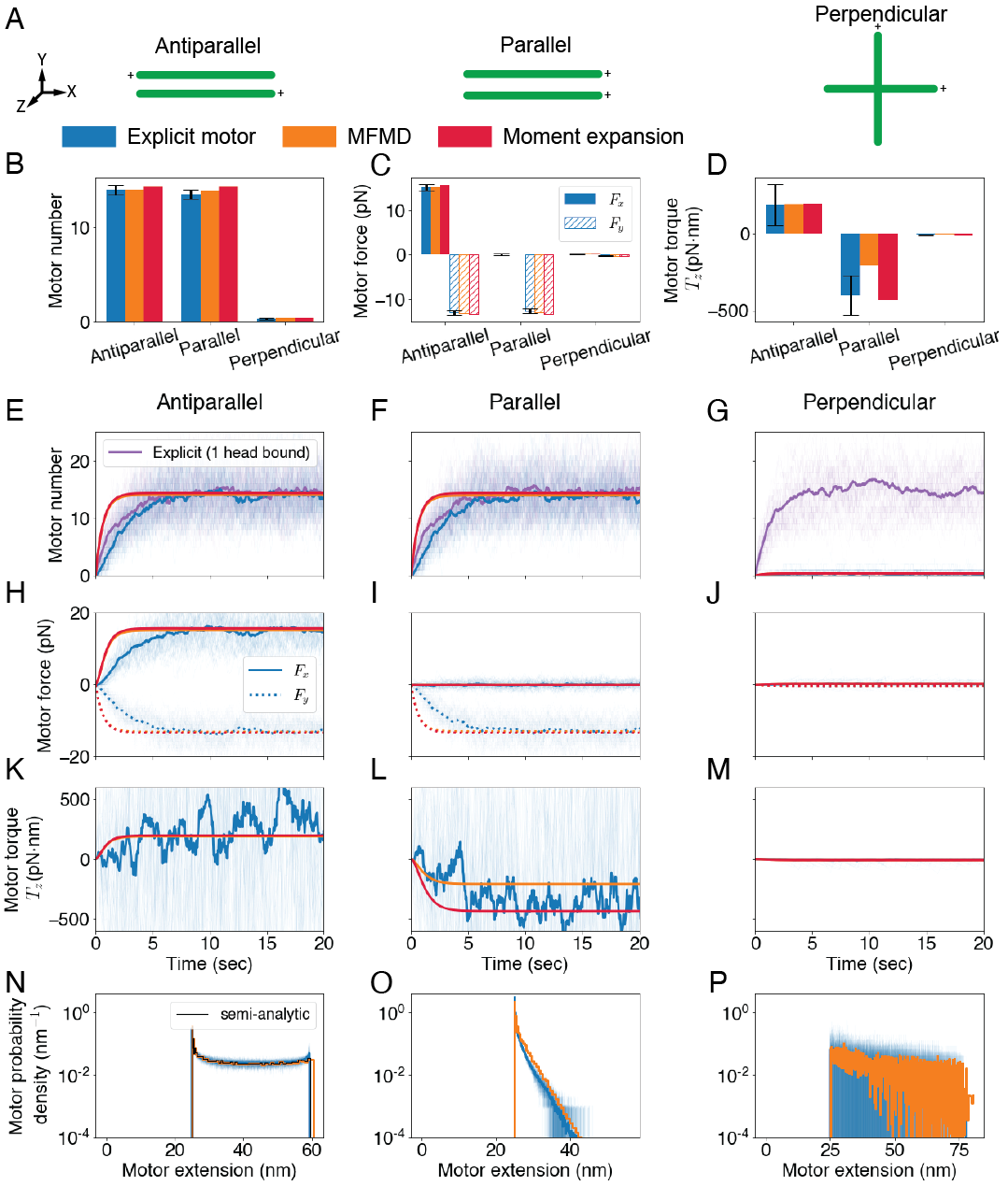
Figure 4: Comparison of model results for three different stationary filament configurations. A Schematic of the three different filament configurations and legend for following plots. B Plot of total crosslink motor numbers at steady state. C Plot of steady-state motor force components from filament $i$ on filament $j$. D Bar graph of steady-state torque in the $\hat{z}$-direction from filament $i$ on filament $j$. Explicit motor model error bars in (B-D) indicate the Standard Error of the Mean (SEM) of the last 30 seconds of 40 second long simulations (n=48). E-G Bound motor number versus time. Purple and blue solid lines are the average of 48 individual explicit motor simulations (translucent lines) for one head bound and crosslinking motors. H-J Motor force in the $\hat{x}$-direction (solid lines) and $\hat{y}$-direction (dotted lines). Individual explicit motor runs are represented as blue for both directions. K-M Motor torque in the $\hat{z}$-direction from filament $i$ on $j$. Full explicit motor model range not shown to better see average. N-P Steady-state motor probability density as a function of motor extension for semi-analytic (black), explicit motor, and MFMD models. Motor minimum extension is set by the separation of filaments at closest point of approach, 25 nm.

When filaments are held stationary, motor density reaches or fluctuates around a steady-state solution (Figure 4). To compare with the mean-field models, we averaged 48 realizations of each explicit motor simulation; the results agreed within error with the mean-field models (Figure 4B-D). This agreement between models demonstrates that the mean-field models capture the average behavior of our explicit model.

Beyond the steady state, we characterize the evolution of motor number, force, and torque (Figure 4E-M). In all configurations, the crosslinking motor number in the explicit motor model lags that of the MFMD and moment expansion models (Figure 4E-G). The crosslinking rate in the two-step binding algorithm depends on the density of motors with one head bound, resulting in a slower approach to steady state.

For antiparallel filaments, force generation increases with crosslinking motor number (Figure 4H, Video 1) because motors walk in opposite directions, causing the motor tether to stretch and generate force. If free to move, these antiparallel filaments would slide. No average sliding would occur for parallel filaments, and the small number of crosslinking proteins for perpendicular filaments results in small relative force (Figure 4I, J). The average explicit motor motor torque in the $\hat{z}$-direction shows significant fluctuations about the mean (Figure 4K-M). Because motor torque increases for motors farther from the filament centers, the torque fluctuations increase with filament length.

We compared the steady-state distribution of motor extension for both explicit motor and MFMD models (Figure 4N-P). (Note that the moment expansion loses this information in coarse-graining.) The distribution of motors crosslinking antiparallel filaments has two peaks (Figure 4N). The larger peak represents the most probable binding distance $\Delta y$, and the second peak corresponds to motors near their stall extension $h=\sqrt{\Delta y^{2}+h_{{\rm stall}}^{2}}$. The shape of the distribution results from motor kinetics, walking, and stalling. Motors on parallel filaments show a peak at $\Delta y$ (Figure 4O, Video 2), but no second peak because the motor heads walk in the same direction with similar speed. For motors crosslinking perpendicular filaments, the extension distribution is singly peaked and broader than for parallel filaments (Figure 4P, Video 3). This occurs because the parallel force component on perpendicular filaments increases more gradually as the motors extend, causing a more gradual decrease in motor speed. This broad distribution indicates a larger average force per motor for perpendicular filaments compared to aligned filaments.

6.2 Dynamical evolution of filament pairs

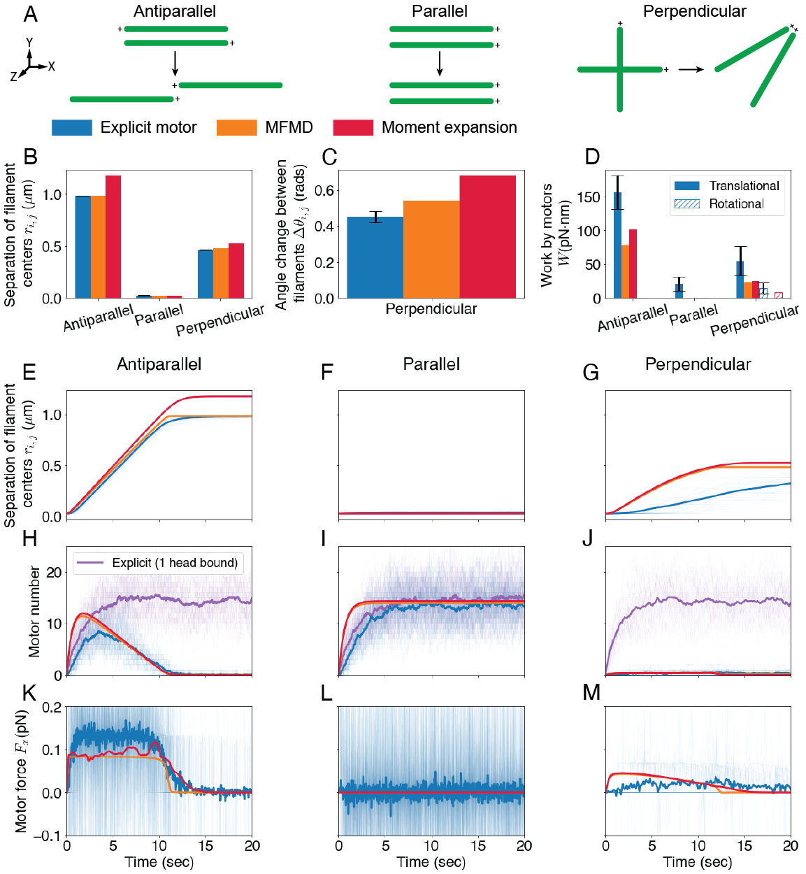
Figure 5: Comparison of model results for three different initial filament configurations evolved with constrained motion. A Schematic of initial and final filament configurations. B Plot of final filament center separations. C Plot of change in angle between filaments starting in a perpendicular configuration. Data shown is final configuration after 100 seconds for the explicit motor model and 20 seconds for MFMD and moment expansion model. D Plot of translational (solid bars) and rotational (hatch bars) work done by motors on filaments during simulation. explicit motor model error bars in (B-D) indicate the SEM of simulation realizations (n=48). E-G Plots of filament centers separation as a function of time. H-J Plots of motor number versus time. Purple and blue solid lines are the average of 48 explicit motor simulations (translucent lines) for one head bound and crosslinking motors. K-M Plots of motor force in the $\hat{x}$-direction with individual explicit motor runs (translucent blue lines) and average (solid blue). Full explicit motor model range not shown to better see average.

Here we consider the same three filament starting configurations and allow filament motion (Figure 5, Videos 4-6). The final filament position and orientation are comparable for the explicit motor and MFMD models, while the moment expansion model overestimates the range of filament translation and rotation (Figure 5B, C; note that filament rotation only occurs for the perpendicular initial configuration).

To compare motor activity between models over the whole simulation, we calculated the total work done by motors. We numerically integrate both filaments using the trapezoid rule [87],

$$W_{{\rm tot}}=W_{{\rm lin}}+W_{{\rm rot}}=\sum_{i\neq j}\int{\bf F}_{i,j}\cdot d{\bf r}_{j}+\sum_{i\neq j}\int{\bf T}_{i,j}\cdot d{\bm{\theta}}_{j},$$ (39)

where $\theta_{j}$ is the angle the vector ${\hat{u}}_{j}$ rotates through over the simulation. The infinitesimal vector $d{\bm{\theta}}_{i}=\hat{\theta}_{i}d\theta_{i}$ where

$$\hat{\theta_{i}}=\frac{{\hat{u}}_{i}\times\dot{{\hat{u}}}_{i}}{|{\hat{u}}_{i}\times\dot{{\hat{u}}}_{i}|}.$$ (40)

Total work computed for the mean-field models is within error of the explicit motor model (Figure 5D). We note that the explicit motor model produces greater total work because fluctuations in motor binding cause fluctuations in sliding direction which generate larger work. Motors generate rotational work only for initially perpendicular filaments, due to the constraints. The magnitude of the rotational work is relatively small because filaments rotate slowly (due to high rotational drag and low motor torque), and this slower velocity produces less work in the overdamped limit.

The crosslinking motor number depends on the filament overlap length, which changes as filaments move (Figure 5E-J). The crosslinking motor number in the explicit motor model lags the mean-field models initially due to differences in binding, but becomes comparable after the initial transient. As antiparallel filaments slide apart, their overlap decreases so fewer motors crosslink, while crosslinking motors continue to unbind at a constant rate. However, the overlap length has little effect on the number of motors with one head bound (Figure 5E, H). The dynamics of motor number for parallel stationary and moving filaments are nearly identical because there is negligible sliding. (Figure 5F, I). Moving perpendicular filaments maintain a similar overlap length to stationary perpendicular filaments, leading to an approximately constant motor number, until the plus-ends move close together (Figure 5G, J). Then motors continue to bind but immediately walk off, producing little force or torque.

The motor force between antiparallel filaments rapidly reaches a force plateau which persists until the antiparallel overlap length is small enough that motor binding is negligible (Figure 5K). The nearly constant force implies that motor extension decreases as the number of crosslinking motors increases to give a constant sliding speed (Figure 5N, Video 4). This steady-state force is an order of magnitude smaller than the stall force (Table 1). The moment expansion model shows a slower decrease in force as the overlap approaches zero compared to the MFMD model (Figure 5H). This is a consequence of our neglect of boundary terms, which physically means neglecting motor dissociation at filament ends. This unphysical slow force decrease drives filaments beyond the zero overlap configuration to larger than expected separation (Figure 5B).

Parallel filaments remain with their centers aligned on average because sampling the full distribution of motor crosslinking extension generates restoring force for any fluctuations away from full overlap (equations 11, 13). Neither the MFMD nor the moment expansion models produce a net force, but in the explicit motor model fluctuations in motor number and binding lead to force and position fluctuations (Figure 5F, I, L, Video 5). For perpendicular filaments, the small number of crosslinking motors results in large force fluctuations in the explicit motor model (Figure 5J). The mean-field models show a rapid increase to half the maximum force of the antiparallel configuration followed by a decrease as the filaments align parallel (Figure 5K, M). The lag caused by the two-step binding model is more apparent here because the explicit lower motor number means filaments move more slowly into the parallel configuration where binding is favored (Video 6).

6.3 Computational cost and accuracy

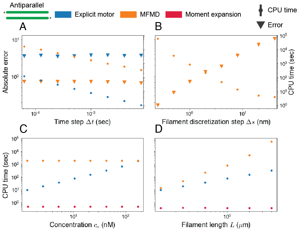
Figure 6: Comparison of computational cost and accuracy of models for stationary filaments in an antiparallel configuration. Error compared against steady-state solution. A Plot of error (triangle) and CPU time (circle) vs time step $\Delta t$ for explicit motor and MFMD models. Each for explicit motor model data point consists of 48 parameter set realizations. MFMD simulations were run 3 times to ensure consistency of time scaling. Standard error of the mean (SEM) of CPU time plotted but not visible. B Plot of error and CPU time vs $\Delta{s}$ for MFMD model. Simulations were run 3 times to ensure consistency. SEM of CPU time plotted but not visible. C, D Plot of CPU time vs unbound motor concentration $c_{o}$ and filament length $L$ for the three models. Explicit motor simulation data points in C and D consist of 24 parameter set realizations while MFMD and moment expansion data points consist of 3 runs for concentration and 4 runs for filament length. SEM of CPU time plotted but not visible.

To compare the accuracy and computational cost of our models, we focus on stationary antiparallel filaments because we can compare to the semi-analytic solution. Antiparallel filaments are also the main configuration in which motors generate extensile force, important for mitotic spindle assembly and dynamics in active nematics. We vary the time step $\Delta t$ and MFMD grid spacing $\Delta{s}$ and compare the error with the semi-analytic solution. The central-processing unit (CPU) time measures the computational cost as a function of simulation parameters.

The solution error is the average magnitude of the deviation of the steady-state numerical solution from $\psi_{i,j}$ of equations (23), (26), and (27),

$${\rm Error}=\int_{L_{i}}\int_{L_{j}}\left|\overline{\psi}_{i,j}-\psi_{i,j}\right|ds_{i}ds_{j}\approx\sum_{m,n}\left|\overline{\psi}_{i,j}(m\Delta{s}_{i},n\Delta{s}_{j})-\psi_{i,j}(m\Delta{s}_{i},n\Delta{s}_{j})\right|\Delta{s}_{i}\Delta{s}_{j},$$ (41)

where $\overline{\psi}_{i,j}$ is either the average explicit motor distribution (over 48 simulations) or the MFMD distribution.

The size of the time step $\Delta t$ does not change the error of explicit motor or MFMD simulations (Figure 6A), because the steady-state solution is time independent. The number of calculations increases linearly with the number of time steps $N_{t}/\Delta t$, making the CPU time approximately inversely proportional to $\Delta t$. The MFMD error scales near-linearly with grid spacing $\Delta{s}$ as expected for a first-order upwind difference method (Figure 6B). The CPU time scales approximately as $\Delta{s}^{-2}$, proportional to the number of grid points $N_{{\rm grid}}\propto\Delta{s}^{-2}$.

Explicit motor simulations have a cost that is linear in the motor number, but the cost is constant for the MFMD and moment expansion models (Figure 6C). Fewer explicit motor simulations (24 realizations) were needed to achieve sufficient statistics. We also note that at higher concentration, the mean-field models return results closer to those of the explicit model because stochastic fluctuations average out. The explicit motor model has a cost linear in filament length (due to the larger number of bound motors on longer filaments), while for the MFMD model it is quadratic (Figure 6D). The cost of the moment expansion model is length independent.

7 Discussion

To improve modeling methods for cytoskeletal filaments crosslinked by motors (Figure 1), we studied crosslinked filament pairs and compared an explicit motor model to two levels of coarse-grained mean-field motor models (Figure 2). The explicit motor model uses Brownian dynamics and kinetic Monte Carlo to describe individual motor binding and unbinding, motion, and force generation. In the first level of coarse graining, we average over individual motors and solve a PDE for the mean-field motor density (MFMD). To further coarse grain, we compute a moment expansion of the MFMD and solve a system of ODEs for the motor moments and filament motion.

We compared the model implementations for filaments that are initially antiparallel, parallel, or perpendicular (Figure 3). When filaments are held stationary, the motor distribution reaches a steady state with similar average motor distribution, force, and torque for the three implementations (Figure 4). The explicit motor simulations showed significant fluctuations that by construction are not present in the mean-field models. Interestingly, we found that a significant portion of crosslinking motors on antiparallel filaments do not reach their stall force for our parameter set.

When filaments move, the final filament separation is similar for the explicit motor and MFMD models, although the moment expansion model overestimates the range of displacement and reorientation as a result of neglecting boundary terms (Figure 5). The dynamics of bound motor number, force, and torque were similar for the MFMD and moment expansion models. Motor fluctuations in the explicit motor model lead to greater overall work done by motors.

To compare computational cost across the model implementations, we studied stationary filaments and motors at steady state (Figure 6). Both mean-field models have a simulation time independent of motor concentration, potentially making them faster than explicit models for systems with many motors. The moment expansion model’s CPU time is also independent of filament length, which could make it particularly efficient for systems with long filaments. Overall, the moment expansion model was $10^{3}-10^{6}$ faster than the other models. This method could therefore be useful for simulating bulk active filament networks.

Future work could address the simplifying assumptions and approximations made in the moment expansion model. An improved treatment of boundary terms may improve the computation of filament motion. Incorporating additional motor physics into the moment expansion model, such as non-zero length motors, force-dependent detachment, and steric interactions between motors could improve its ability to simulate microscopic motor behavior at the mesoscale, bridging current explicit motor and continuous active network theories. Implementing the moment expansion model in systems of many filaments is of interest for testing whether the improvements in computational cost we identify are present in larger systems.

Appendix A Determining the time-step for binding

Our kinetic Monte Carlo algorithm assumes that multiple binding/unbinding events do not occur in the same time step $\Delta t$. As $\Delta t$ becomes large relative to the kinetic rates, this approximation fails. A time step is appropriate if the maximum probability of two events occurring in $\Delta t$ satisfies

$$\max\{P(C(\Delta t)\cup B(t^{\prime})|A(0))\}<\delta$$ (42)

for a tolerance $\delta$, where $A,B$, and $C$ denote motor bound states (including unbound, single head bound, and crosslinking) at time $\Delta t>t^{\prime}>0$. $P(C(\Delta t)\cup B(t^{\prime})|A(0))=P(C(\Delta t)|B(t^{\prime}))P(B(t^{\prime})|A(0))$ and each individual state change follows a single event Poisson process with $P(B(t)|A(0))=1-\exp[-k_{A\to B}t]$. The maximum probability for a double event occurs at $t^{\prime}=t^{\prime}_{\rm{max}}$ found by solving

$$\begin{split}\frac{dP(C(\Delta t)\cup B(t^{\prime})|A(0))}{dt^{\prime}}\Bigg{|}_{t^{\prime}_{max}}&=0\\ k_{A\to B}\left(e^{k_{B\to C}(\Delta t-t^{\prime})}-1\right)-k_{B\to C}\left(e^{k_{A\to B}t^{\prime}}-1\right)&=0.\end{split}$$ (43)

While no analytic solution exists, $t^{\prime}_{\rm{max}}$ can be numerically computed.

There are four unique processes that must be considered with a two-step binding process with unbound (U), single head bound (S), and crosslinking (C) states: $U\to S\to U$, $U\to S\to C$, $S\to C\to S$, and $C\to S\to U$. The process $C\to S\to C$ has the same probability as $S\to C\to S$, similarly, $S\to U\to S$ has the same probability as $U\to S\to U$. If modeling filament motion with some force- or energy-dependent unbinding, $k_{{\rm off},d}$ may be large. This means that in the limit of large unbinding rate the probabilities $P(C\to S\to C)\to P(S\to C)$ and $P(C\to S\to U)\to P(S\to U)$.

Appendix B Lookup table for kinetic Monte Carlo binding

Equation (11) gives the transition probability of a singly bound motor crosslinking as an integral of a Boltzmann factor. If $h_{\rm cl}=0$, $k_{{\rm on},C}$ is functionally similar to an error function. However, to model non-zero-length tethers, we numerically integrate equation (11). Rather than directly numerically integrating at each time step, we precompute a lookup table.

The cumulative distribution function (CDF) of equation (11), is a function $h_{i,j}$. All other variables in the integral are constant for a given motor species. We reduce the CDF dimensionality by considering the lab position of each bound motor head and an infinite carrier line defined by the position and orientation of the unbound filament. Binding is then determined by the minimum distance $r_{\perp}$ between the bound motor head position and the filament ends $[s_{-},s_{+}]$ on the carrier line.

The carrier line CDF is

$$\operatorname{{\rm CDF}}(r_{\perp},s)=\int_{-\infty}^{s}e^{-\beta U(r_{\perp},s^{\prime})}ds^{\prime},$$ (44)

allowing us to write the crosslinking rate as

$$k_{{\rm on},C}(r_{\perp},s_{+},s_{-})=k_{{\rm o},d}\epsilon K_{\rm E}\left[\operatorname{{\rm CDF}}(r_{\perp},s_{+})-\operatorname{{\rm CDF}}(r_{\perp},s_{-})\right].$$ (45)

We notice that $e^{-\beta U_{i,j}}$ is symmetric in $s$, so $\operatorname{{\rm CDF}}(r_{\perp},s)-\operatorname{{\rm CDF}}(r_{\perp},0)$ is anti-symmetric. Therefore, instead of integrating from negative infinity, we use

$$\operatorname{{\rm CDF}}^{\prime}(r_{\perp},s)=\operatorname{sgn}(s)\int_{0}^{s}e^{-\beta U(r_{\perp},s^{\prime})}ds^{\prime}$$ (46)

and (45) to find the crosslinking rate.

We find the values of equation (46) by Gauss-Konrad integration. The accuracy desired sets the maximum values for $s$ and $r_{\perp}$. The integrand is always positive for real values of $s$ and $r_{\perp}$, so the CDF asymptotes for large values of either variable. The maximum of the integral is the point when the Boltzmann factor drops to the accuracy limit $\delta$. Therefore, the lookup table domain is

$$s,r_{\perp}\in\left[0,\sqrt{-\frac{2\ln(\delta)}{\beta k_{\rm cl}}}+h_{\rm cl}\right].$$ (47)

Given a specified grid spacing $\Delta s,\Delta r$, the memory required for the lookup table scales as $(s_{\max}/\Delta s)\times(r_{\perp,\max}/\Delta r)$

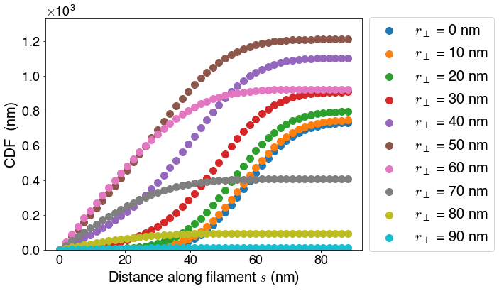
Figure 7: Visual representation of the lookup table showing CDF values as a function of distance $s$ along the filament for $h_{\rm cl}=32$ nm, $k_{\rm cl}=.3$ pN/nm, $\beta=1./4.11$ (pN$\cdot$nm)^-1, and $\delta=10^{-5}$.

B.1 Interpolation of lookup table values

Since the lookup table is not a continuous function, we interpolate values between discrete grid points. The 2D linear interpolation for input values of $r_{\perp}$ and $s$ is

$$\begin{split}\operatorname{{\rm CDF}}(r_{\perp},s)\approx&\left(1+m-\frac{r_{\perp}}{\Delta r}\right)\left(1+n-\frac{s}{\Delta s}\right)\operatorname{{\rm CDF}}_{m,n}+\left(\frac{r_{\perp}}{\Delta r}-m\right)\left(1+n-\frac{s}{\Delta s}\right)\operatorname{{\rm CDF}}_{m+1,n}\\ +&\left(1+m-\frac{r_{\perp}}{\Delta r}\right)\left(\frac{s}{\Delta s}-n\right)\operatorname{{\rm CDF}}_{m,n+1}+\left(\frac{r_{\perp}}{\Delta r}-m\right)\left(\frac{s}{\Delta s}-n\right)\operatorname{{\rm CDF}}_{m+1,n+1},\end{split}$$ (48)

where $\operatorname{{\rm CDF}}_{m,n}=\operatorname{{\rm CDF}}(m\Delta r,n\Delta s)$ are the lookup table values at $m$ and $n$ if $r_{\perp}$ lies within $m\Delta r$ and $(m+1)\Delta r$ and $s$ lies within $n\Delta s$ and $(n+1)\Delta s$.

B.2 Reverse lookup algorithm

When a motor head binds to a filament, the binding position probability distribution function (PDF) is defined by the Boltzmann factor. We sample the PDF by using the lookup table. To transform a uniform random variable $X$ to random variable $Y$ with an arbitrary $\operatorname{{\rm PDF}}_{Y}$, $X$ is inserted into the inverted CDF of $Y$

$$Y=\operatorname{{\rm CDF}}_{Y}^{-1}(X).$$ (49)

Since the lookup table holds the CDF values and given a random number from a uniform distribution, we apply a combination of search and interpolation to quickly find the corresponding random number from the PDF. The algorithm is as follows

1. Sample a uniform random number $X\in[0,\operatorname{{\rm CDF}}_{\max}]$. Note that the maximum value does not need to be 1.

2. Given $r_{\perp}$, locate index $m$ such that $m\Delta r\leq r_{\perp}\leq(m+1)\Delta r$

3. Use $m$ to find the set of indices $\{n_{-},n_{+}\}$ such that $\operatorname{{\rm CDF}}_{m,n_{-}}\leq X\leq\operatorname{{\rm CDF}}_{m,n_{-}+1}$ and $\operatorname{{\rm CDF}}_{m+1,n_{+}}\leq X\leq\operatorname{{\rm CDF}}_{m+1,n_{+}+1}$.

4. Use the CDF values to interpolate the binding locations $s_{-},s_{+}$ corresponding to the perpendicular distances $r_{-}=m\Delta r$ and $r_{+}=(m+1)\Delta r$. For example,

   $$s_{-} =\Delta s\frac{X-\operatorname{{\rm CDF}}_{m,n_{-}}}{\operatorname{{\rm CDF}}_{m,n_{-}+1}-\operatorname{{\rm CDF}}_{m,n_{-}}}+\Delta sn_{-}$$ (50)

   $$s_{+} =\Delta s\frac{X-\operatorname{{\rm CDF}}_{m+1,n_{+}}}{\operatorname{{\rm CDF}}_{m+1,n_{+}+1}-\operatorname{{\rm CDF}}_{m+1,n_{+}}}+\Delta sn_{+}$$ (51)

   Note that $s_{-}$ is not necessarily less than $s_{+}$.

5. Find $s$ by interpolating the across the lookup table grid with respect to $r_{\perp}$

   $$s\approx(s_{+}-s_{-})\frac{r_{\perp}-r_{-}}{\Delta r}+s_{-}$$ (52)

While this algorithm succeeds in most circumstance, the low slope of the CDF at large values of $s$ can cause errors. For example, if the lookup table has the form of Figure 7 and a protein is located at a perpendicular distance of $r_{\perp}=35$ nm, given a random number of $X=10^{3}$, no value for $s_{-}$ will be found since $\operatorname{{\rm CDF}}(30,s_{\rm max})<10^{3}$. To correct for this, we solve for $s$ using a binary search algorithm.

The binary search algorithm is as follows

1. Determine if $\operatorname{{\rm CDF}}_{m,n_{\rm max}}$ or $\operatorname{{\rm CDF}}_{m+1,n_{\rm max}}$ is less than $X$. If $\operatorname{{\rm CDF}}_{m,n_{\rm max}}<X$, set $s_{-}=s_{\rm max}$. If $\operatorname{{\rm CDF}}_{m+1,n_{\rm max}}<X$, set $s_{+}=s_{\rm max}$.

2. Find other $s_{\pm}$ using the inverted lookup table and equation (50) or (51).

3. Find the average of $s_{-}$ and $s_{+}$.

4. Use the lookup table interpolation algorithm to find the $\operatorname{{\rm CDF}}(r_{\perp},s_{\rm avg})$.

5. If $\operatorname{{\rm CDF}}(r_{\perp},s_{\rm avg})>X$ set the larger of the two $s_{\pm}$ values to $s_{\rm avg}$. Otherwise, set the smaller of the two to $s_{\rm avg}$.

6. Repeat steps 3-5 until $|\operatorname{{\rm CDF}}(r_{\perp},s_{\rm avg})-X|<\delta$ for some desired tolerance $\delta$.

This process converges at a rate $O(\log_{2}(\delta s_{\max}))$.

Appendix C Numerical integration of the MFMD equation

We approximate the solution $\psi_{i,j}(s_{i},s_{j},t)$ by discretizing the solution in time and space

$$\psi_{i,j}(s_{i},s_{j},t)\to\psi_{i,j}^{m,n,k}=\psi_{i,j}(m\Delta{s},n\Delta{s},k\Delta t)$$ (53)

for $\psi_{i,j}^{m,n,k}{}\in\mathbb{R}^{(M_{i}+1)\times(M_{j}+1)\times k}$, where $M_{i}$ is the number of discretized points along filament $i$. Additional boundary points for $m,n=0$ are added.

We use forward Euler time-stepping so our discrete differential operator for time is

$$\frac{\partial\psi_{i,j}}{\partial t}\to\frac{1}{\Delta t}(\psi_{i,j}^{m,n,k}-\psi_{i,j}^{m,n,k-1}).$$ (54)

To solve the hyperbolic FPE (17), we use a first-order accurate upwind method[88]. The differential operator for $s_{i}$ becomes

$$\frac{\partial\psi_{i,j}}{\partial s_{i}}\to\frac{1}{\Delta{s}}(\psi_{i,j}^{m,n,k}-\psi_{i,j}^{m-1,n,k}).$$ (55)

Note this only holds for the indices $0<m$ and $0<n$. The matrix representation for equation (55) is

$$\frac{1}{\Delta s}\begin{pmatrix}c_{0}&c_{1}&c_{2}&\cdots&c_{M_{i}}\\ -1&1&0&&\\ 0&-1&1&\ddots&\\ \vdots&&\ddots&\ddots&0\\ d_{0}&\cdots&&d_{M_{i}-1}&d_{M_{i}}\end{pmatrix}\begin{pmatrix}\psi_{i,j}^{0,n,k}{}\\ \psi_{i,j}^{1,n,k}{}\\ \vdots\\ \psi_{i,j}^{M_{i}-1,n,k}{}\\ \psi_{i,j}^{M_{i},n,k}{}\end{pmatrix}=\rhd^{m,a}\psi_{i,j}^{a,n,k},$$ (56)

where $c_{m}$ and $d_{m}$ are chosen to satisfy the boundary conditions. We choose the notation $\rhd^{m,n}$ for this matrix. To differentiate along $s_{j}$, we use the identity $\psi_{i,j}^{m,n,k}=\psi_{j,i}^{n,m,k}$, apply $\rhd^{m,n}$ on the matrix, and then convert back,

$$\frac{\partial\psi_{i,j}}{\partial s_{i}}\to\left(\sum_{a}\rhd^{n,a}\psi_{j,i}^{a,m}\right)^{T},$$ (57)

which in index notation is $\psi_{i,j}^{m,a}(\rhd^{T})^{n,a}$. For brevity, we use the notation $\psi_{i,j}^{m,a}(\rhd^{T})^{n,a}=\psi_{i,j}^{m,a}\lhd^{a,n}$.

The discretized Fokker-Planck equation (17) is then

$$\psi_{i,j}^{m,n,k+1}=\Delta t\left(-\rhd^{m,a}\left(v_{i,j}^{a,n,k}\psi_{i,j}^{a,n,k}\right)-\left(v_{j,i}^{m,a,k}\psi_{i,j}^{m,a,k}\right)\lhd^{a,n}+2k_{{\rm o}}ce^{-\beta U_{i,j}^{m,n,k}}-2k_{{\rm o}}\psi_{i,j}^{m,n,k}\right)+\psi_{i,j}^{m,n,k}{},$$ (58)

where $U_{i,j}^{m,n,k}$ and $v_{i,j}^{m,n,k}$ are the discretized potential and velocity at time $k\Delta t$. Note that $U_{i,j}^{m,n,k}=U_{j,i}^{n,m,k}$, but $v_{i,j}^{m,n,k}\neq v_{j,i}^{n,m,k}$.

In cases where the flux of the motors $\frac{\partial\left(v_{i,j}\psi_{i,j}\right)}{\partial s_{i}}$ is known at the boundaries, we construct $\rhd$ to satisfy the requirements. When filaments are in solution, there is zero flux from the minus ends, so all $c_{m}=0$. In our simulations, motors walk of filament ends with out pausing, so $d_{M_{i}-1}=-1$ and $d_{M_{i}}=1$ with all other $d_{m}=0$. Although not modeled in this paper, some biological motors end pause at filament plus ends. To model this, $d_{M_{i}-1}=-1$ and every other $d_{m}=0$.

Appendix D Conversion of binding parameters from an explicit to mean-field motor density model

To relate binding parameters of the one-step and multi-step binding models, we use that at steady state, the motor distribution $\psi_{i,j}$ should be equivalent for both models. Since we only compare binding kinetics, we simplify the Fokker-Planck equation to keep only the binding terms: in equation (17), we set $v_{i,j}=v_{j,i}=0$,

$$\frac{\partial\psi_{i,j}}{\partial t}=2k_{{\rm o}}ce^{-\beta U_{i,j}}-2k_{{\rm o}}\psi_{i,j}.$$ (59)

The steady-state solution is

$$\psi_{i,j}=ce^{-\beta U_{i,j}},$$ (60)

which is a Boltzmann factor multiplied by an effective concentration.

The multi-step binding model can be written

$$\begin{split}\frac{\partial\psi_{i,j}(s_{i},s_{j})}{\partial t}&=\epsilon K_{\rm E}^{\prime}k_{{\rm o},C}(\chi_{i}+\chi_{j})e^{-\beta U_{i,j}}-2k_{{\rm o},C}\psi_{i,j},\end{split}$$ (61)

$$\begin{split}\frac{\partial\chi_{i}(s_{i})}{\partial t}&=c_{o}K_{a}\epsilon k_{{\rm o},S}-k_{{\rm o},S}\chi_{i}+\int_{L_{j}}\left(k_{{\rm o},C}\psi_{i,j}-\epsilon K_{\rm E}^{\prime}k_{{\rm o},C}\chi_{i}e^{-\beta U_{i,j}}\right)ds_{j},\end{split}$$ (62)

$$\begin{split}\frac{\partial\chi_{j}(s_{j})}{\partial t}&=c_{o}K_{a}\epsilon k_{{\rm o},S}-k_{{\rm o},S}\chi_{j}+\int_{L_{i}}\left(k_{{\rm o},C}\psi_{i,j}-\epsilon K_{\rm E}^{\prime}k_{{\rm o},C}\chi_{j}e^{-\beta U_{i,j}}\right)ds_{i},\end{split}$$ (63)

where $\chi_{i}$ is the mean-field density of motors with one head bound to filament $i$ (cf. Equation 16). We define $K_{\rm E}^{\prime}=K_{\rm E}/V_{\rm bind}$ and solve for the steady state, giving

$$\begin{split}\psi_{i,j}&=\frac{\epsilon K_{\rm E}^{\prime}}{2}(\chi_{i}+\chi_{j})e^{-\beta U_{i,j}},\end{split}$$ (64)

$$\begin{split}\chi_{i}&=\frac{\epsilon K_{\rm E}^{\prime}k_{{\rm o},C}}{2k_{{\rm o},S}}\left(\int_{L_{j}}(\chi_{j}-\chi_{i})e^{-\beta U_{i,j}}ds_{j}\right)+\epsilon K_{a}c_{o},\end{split}$$ (65)

$$\begin{split}\chi_{j}&=\frac{\epsilon K_{\rm E}^{\prime}k_{{\rm o},C}}{2k_{{\rm o},S}}\left(\int_{L_{i}}(\chi_{i}-\chi_{j})e^{-\beta U_{i,j}}ds_{i}\right)+\epsilon K_{a}c_{o}.\end{split}$$ (66)

The equations for $\chi_{i}$ and $\chi_{j}$ have the forms

$$\begin{split}X(s)&=C\int_{a}^{b}\left(Y(t)-X(s)\right)K(s,t)dt+D,\end{split}$$ (67)

$$\begin{split}Y(t)&=C\int_{c}^{d}\left(X(s)-Y(t)\right)K(s,t)ds+D,\end{split}$$ (68)

where $t\in[a,b]$ and $s\in[c,d]$. Distributing the integrals, we can rewrite

$$\begin{split}X(s)&=C\int_{a}^{b}Y(t)K(s,t)dt-CX(s)F(s)+D,\end{split}$$ (69)

$$\begin{split}Y(t)&=C\int_{c}^{d}X(s)K(s,t)ds-CY(t)G(t)+D,\end{split}$$ (70)

where $F(s)=\int_{a}^{b}K(s,t)dt$ and $G(t)=\int_{c}^{d}K(s,t)ds$. Solving for $X(s)$ and $Y(t)$ gives

$$\begin{split}X(s)&=\frac{D}{1+CF(s)}+\frac{C}{1+CF(s)}\int_{a}^{b}Y(t)K(s,t)dt,\end{split}$$ (71)

$$\begin{split}Y(t)&=\frac{D}{1+CG(t)}+\frac{C}{1+CG(t)}\int_{c}^{d}X(s)K(s,t)ds,\end{split}$$ (72)

After plugging equation (71) into (72) we find

$$Y(t)=\frac{D}{1+CG(t)}+\frac{CD}{1+CG(t)}\int_{c}^{d}\frac{K(s,t)}{1+CF(s)}ds+C^{2}\int_{a}^{b}\int_{c}^{d}Y(t^{\prime})\frac{K(s,t)K(s,t^{\prime})}{(1+CF(s))(1+CG(t^{\prime}))}dsdt^{\prime}.$$ (73)

This can be rearranged into the form

$$Y(t)=A(t)+\int_{a}^{b}Y(t^{\prime})B(t,t^{\prime})dt^{\prime},$$ (74)

which implies that $Y(t)$ and $X(s)$ each satisfy a Fredholm equation of the second kind. Both $A$ and $B$ are continuous given $K(s,t)=e^{-\beta U_{i,j}(s,t)}$, so the Fredholm equations of the second kind have unique solutions. By inspection, the solution to equations (67) and (68) is $X(s)=Y(t)=D$. When we substitute this solution in equations (65) and (66), we find $\chi_{i}=\chi_{j}=\epsilon K_{a}c_{o}$ and

$$\psi_{i,j}=\epsilon^{2}K_{a}K_{\rm E}^{\prime}c_{o}e^{-\beta U_{i,j}}.$$ (75)

Setting equation (60) equal to (75) gives

$$c=\frac{\epsilon^{2}K_{a}K_{\rm E}}{V_{\rm bind}}c_{o}.$$ (76)

Appendix E Calculating binding parameters from experiments

The experimental parameters for motor binding are not always independently measured. If all but one binding parameters are known, then the unknown parameter can be found from equation (18) and the ratio of the number of motors with one head bound and number of motors crosslinking.

As an example, suppose we wish to find $K_{\rm E}$. The number of motors with one head bound is $N_{S}=c_{o}K_{a}\epsilon L$, where $L$ is the filament length. In vitro experiments [86] can measure the crosslinking motors number $N_{d}$. Integrating equation (75), we the model prediction for the number of crosslinking motors is

$$N_{C}=c_{o}\epsilon^{2}K_{a}K_{\rm E}^{\prime}\int_{L_{i}}\int_{L_{j}}e^{-\beta U_{i,j}}ds_{i}ds_{j}.$$ (77)

For fully parallel or antiparallel filaments of the same length with adjacent centers, the total number of motors in equation (77) is proportional to $L$. If $L\gg\sqrt{2/\beta k_{\rm cl}}$, the Gaussian integral $\approx L\sqrt{2\pi/\beta k_{\rm cl}}e^{-\beta k_{\rm cl}r_{\perp}^{2}}$, where $r_{\perp}$ is the center-to-center separation between filaments. The ratio of the number of crosslinking motors relative to the number motors with one head bound is

$$\rho=\frac{N_{C}}{N_{S}}=\epsilon K_{\rm E}^{\prime}\sqrt{\frac{2\pi}{\beta k_{\rm cl}}}e^{-\beta k_{\rm cl}r_{\perp}^{2}},$$ (78)

allowing us to estimate $K_{\rm E}^{\prime}=\frac{\rho}{\epsilon}\sqrt{\frac{\beta k_{\rm cl}}{2\pi}}e^{\beta k_{\rm cl}r_{\perp}^{2}}$.

Appendix F Gaussian integrals in the moment expansion

The source terms in the moment expansion require a double integral over two filaments. To lower the numerical integration’s computational cost, we find an analytic solution for either the semi-integrated term $Q_{j}^{l}(s_{i})$ or the fully-integrated term $q_{i,j}^{k,l}$.

The integrated source terms are

$$\begin{split}q_{i,j}^{k,l}=ce^{-\left(\frac{r}{\alpha}\right)^{2}}&\Bigg{\{}\int_{L_{i}}s_{i}^{k}\exp\left[-\frac{s_{i}^{2}-2s_{i}{\bf r}_{i,j}\cdot{\hat{u}}_{i}-({\bf r}_{j,i}\cdot{\hat{u}}_{j}+{\hat{u}}_{i}\cdot{\hat{u}}_{j}s_{i})^{2}}{\alpha^{2}}\right]\\ &\int_{L_{j}}s_{j}^{l}\exp\left[-\left(\frac{s_{j}-{\bf r}_{j,i}\cdot{\hat{u}}_{j}-{\hat{u}}_{i}\cdot{\hat{u}}_{j}s_{i}}{\alpha}\right)^{2}\right]ds_{j}ds_{i}\Bigg{\}},\end{split}$$ (79)

where $\alpha=\sqrt{\frac{2}{\beta k_{\rm cl}}}$. We define the quantity $A=-{\bf r}_{j,i}\cdot{\hat{u}}_{j}-{\hat{u}}_{i}\cdot{\hat{u}}_{j}s_{i}$ so that the integral over $s_{j}$ becomes

$$\bar{Q}^{l}_{j}(s_{i})=\int_{L_{j}}s_{j}^{l}e^{-{\left(\frac{s_{j}+A}{\alpha}\right)}^{2}}ds_{j}.$$ (80)

This integral has an analytic form in terms of error functions, which can be rapidly computed. For $l={0,1,2,3}$, we find

$$\bar{Q}_{j}^{0}(s_{i})=\frac{\alpha\sqrt{\pi}}{2}\left[\operatorname{erf}\left(\frac{s_{j}+A}{\alpha}\right)\right]_{\partial L_{j}}$$ (81)

$$\bar{Q}_{j}^{1}(s_{i})=-\frac{\alpha}{2}\left[\alpha e^{-\left(\frac{s_{j}+A}{\alpha}\right)^{2}}+A\sqrt{\pi}\operatorname{erf}\left(\frac{s_{j}+A}{\alpha}\right)\right]_{\partial L_{j}}$$ (82)

$$\bar{Q}_{j}^{2}(s_{i})=\frac{\alpha}{4}\left[2\alpha(A-s_{j})e^{-\left(\frac{s_{j}+A}{\alpha}\right)^{2}}+(2A^{2}+\alpha^{2})\sqrt{\pi}\operatorname{erf}\left(\frac{s_{j}+A}{\alpha}\right)\right]_{\partial L_{j}}$$ (83)

$$\bar{Q}_{j}^{3}(s_{i})=\frac{-\alpha}{4}\left[2\alpha(A^{2}-As_{j}+s_{j}^{2}+\alpha^{2})e^{-\left(\frac{s_{j}+A}{\alpha}\right)^{2}}+(2A^{2}+3\alpha^{2})A\sqrt{\pi}\operatorname{erf}\left(\frac{s_{j}+A}{\alpha}\right)\right]_{\partial L_{j}}$$ (84)

Appendix G Moment expansion boundary terms

To generally define boundary conditions, instead of integrating over both $s_{i}$ and $s_{i}$, we integrate over just one variable. This makes the boundary condition a function of a single filament attatchment position. For example, the boundary terms for the first filament are

$$\begin{split}\dot{B}_{j}^{l}(s_{i})=\int_{L_{j}}&\left(2k_{{\rm o}}ce^{-\beta U_{i,j}}+(2\kappa-2k_{{\rm o}})\psi_{i,j}-\left(v_{o}+\kappa({\bf r}_{i,j}\cdot{\hat{u}}_{i}+{\hat{u}}_{i}\cdot{\hat{u}}_{j}s_{j}-s_{i})\right)\frac{\partial\psi_{i,j}}{\partial s_{i}}\right.\\ &\left.-\left(v_{o}+\kappa({\bf r}_{j,i}\cdot{\hat{u}}_{j}+{\hat{u}}_{i}\cdot{\hat{u}}_{j}s_{i}-s_{j})\right)\frac{\partial\psi_{i,j}}{\partial s_{j}}\right)s_{j}^{l}ds_{j}.\end{split}$$ (85)

These boundary terms are evaluated at $-L_{i}/2$ and $L_{i}/2$. We derive a recursion relation by integrating equation (85) over $s_{j}$ and using the definition in equation (37)

$$\begin{split}\dot{B}_{j}^{l}\left(s_{i}\right)&=2k_{{\rm o}}cQ_{j}^{l}\left(s_{i}\right)+l\left(v_{o}+\kappa({\bf r}_{j,i}\cdot{\hat{u}}_{j}+{\hat{u}}_{i}\cdot{\hat{u}}_{j}s_{i})\right)B_{j}^{l-1}-\left(2k_{{\rm o}}+\kappa(l-1)\right)B_{j}^{l}\\ &-\left(v_{o}+\kappa({\bf r}_{i,j,j}\cdot{\hat{u}}_{i,j}-s_{i})\right)\frac{\partial B_{j}^{l}}{\partial s_{i}}-\kappa{\hat{u}}_{i}\cdot{\hat{u}}_{j}\frac{\partial B_{j}^{l+1}}{\partial s_{i}}\\ &-\left[s_{j}^{l}\left(v_{o}+\kappa\left({\bf r}_{j,i}\cdot{\hat{u}}_{j}+{\hat{u}}_{i}\cdot{\hat{u}}_{j}s_{i}-s_{j}\right)\right)\psi_{i,j}\left(s_{i},s_{j}\right)\right]_{\partial L_{j}}.\end{split}$$ (86)

Solving this equation requires finding the time evolution of the boundary term spatial derivatives, which solve

$$\begin{split}\frac{\partial\dot{B}_{j}^{l}\left(s_{i}\right)}{\partial s_{i}}&=2k_{{\rm o}}c\frac{\partial Q_{j}^{l}}{\partial s_{i}}+{\hat{u}}_{i}\cdot{\hat{u}}_{j}lB_{j}^{l-1}\\ &+l\left(v_{o}+\kappa({\bf r}_{j,i}\cdot{\hat{u}}_{j}+{\hat{u}}_{i}\cdot{\hat{u}}_{j}s_{i})\right)\frac{\partial B_{j}^{l-1}}{\partial s_{i}}-\left(2k_{{\rm o}}+\kappa(l-2)\right)\frac{\partial B_{j}^{l}}{\partial s_{i}}\\ &-\left(v_{o}+\kappa({\bf r}_{i,j,j}\cdot{\hat{u}}_{i,j}-s_{i})\right)\frac{\partial^{2}B_{j}^{l}}{\partial s_{i}^{2}}+\kappa{\hat{u}}_{i}\cdot{\hat{u}}_{j}\frac{\partial^{2}B_{j}^{l+1}}{\partial s_{i}^{2}}\\ &+\textrm{corner terms}.\end{split}$$ (87)

This shows that the boundary terms do not close. However, if the higher-order terms or their coefficients are small compared to the moments $\mu_{i,j}^{k,l}$, we may take a zeroth-order approximation. We consider this approximation in Section 6.

References

- [1] Jonathon Howard. Mechanics of Motor Proteins and the Cytoskeleton. Sinauer Associates, Publishers, Sunderland, Mass, 2001.
- [2] Dennis Bray. Cell Movements: From Molecules to Motility. Garland Pub, New York, 2nd ed edition, 2001.
- [3] Laurent Blanchoin, Rajaa Boujemaa-Paterski, Cécile Sykes, and Julie Plastino. Actin Dynamics, Architecture, and Mechanics in Cell Motility. Physiological Reviews, 94(1):235–263, January 2014.
- [4] Thomas D. Pollard and John A. Cooper. Actin, a Central Player in Cell Shape and Movement. Science, 326(5957):1208–1212, November 2009.
- [5] J. Richard McIntosh, Maxim I. Molodtsov, and Fazly I. Ataullakhanov. Biophysics of mitosis. Quarterly Reviews of Biophysics, 45(2):147–207, May 2012.
- [6] AF. HUXLEY. Muscle structure and theories of contraction. Prog. Biophys. Biophys. Chem, 7:255–318, 1957.
- [7] A. F. Huxley and S. Tideswell. Filament compliance and tension transients in muscle. Journal of Muscle Research & Cell Motility, 17(4):507–511, August 1996.
- [8] A. F. HUXLEY and S. TIDESWELL. Rapid regeneration of power stroke in contracting muscle by attachment of second myosin head. Journal of Muscle Research & Cell Motility, 18(1):111–114, February 1997.
- [9] Stephanie L. Gupton and Clare M. Waterman-Storer. Spatiotemporal Feedback between Actomyosin and Focal-Adhesion Systems Optimizes Rapid Cell Migration. Cell, 125(7):1361–1374, June 2006.
- [10] Maxime F. Fournier, Roger Sauser, Davide Ambrosi, Jean-Jacques Meister, and Alexander B. Verkhovsky. Force transmission in migrating cells. Journal of Cell Biology, 188(2):287–297, January 2010.
- [11] Erin L. Barnhart, Kun-Chun Lee, Kinneret Keren, Alex Mogilner, and Julie A. Theriot. An Adhesion-Dependent Switch between Mechanisms That Determine Motile Cell Shape. PLOS Biology, 9(5):e1001059, May 2011.
- [12] G. Laevsky. Cross-linking of actin filaments by myosin II is a major contributor to cortical integrity and cell motility in restrictive environments. Journal of Cell Science, 116(18):3761–3770, September 2003.
- [13] Iain Hagan and Mitsuhiro Yanagida. Kinesin-related cut 7 protein associates with mitotic and meiotic spindles in fission yeast. Nature, 356(6364):74, March 1992.
- [14] W. S. Saunders, D. Koshland, D. Eshel, I. R. Gibbons, and M. A. Hoyt. Saccharomyces cerevisiae kinesin- and dynein-related proteins required for anaphase chromosome segregation. Journal of Cell Biology, 128(4):617–624, February 1995.
- [15] Tarun M. Kapoor, Thomas U. Mayer, Margaret L. Coughlin, and Timothy J. Mitchison. Probing Spindle Assembly Mechanisms with Monastrol, a Small Molecule Inhibitor of the Mitotic Kinesin, Eg5. Journal of Cell Biology, 150(5):975–988, September 2000.
- [16] Shang Cai, Lesley N. Weaver, Stephanie C. Ems-McClung, and Claire E. Walczak. Kinesin-14 Family Proteins HSET/XCTK2 Control Spindle Length by Cross-Linking and Sliding Microtubules. Molecular Biology of the Cell, 20(5):1348–1359, December 2008.
- [17] Roy Wollman, Gul Civelekoglu-Scholey, Jonathan M Scholey, and Alex Mogilner. Reverse engineering of force integration during mitosis in the Drosophila embryo. Molecular Systems Biology, 4(1):195, January 2008.
- [18] Gul Civelekoglu-Scholey and Jonathan M. Scholey. Mitotic force generators and chromosome segregation. Cellular and Molecular Life Sciences, 67(13):2231–2250, July 2010.
- [19] Zhen-Yu She and Wan-Xi Yang. Molecular mechanisms of kinesin-14 motors in spindle assembly and chromosome segregation. Journal of Cell Science, 130(13):2097–2110, July 2017.
- [20] Kruno Vukušić, Renata Buda, Agneza Bosilj, Ana Milas, Nenad Pavin, and Iva M. Tolić. Microtubule Sliding within the Bridging Fiber Pushes Kinetochore Fibers Apart to Segregate Chromosomes. Developmental Cell, 43(1):11–23.e6, October 2017.
- [21] Sujoy Ganguly, Lucy S. Williams, Isabel M. Palacios, and Raymond E. Goldstein. Cytoplasmic streaming in Drosophila oocytes varies with kinesin activity and correlates with the microtubule cytoskeleton architecture. Proceedings of the National Academy of Sciences, 109(38):15109–15114, September 2012.
- [22] Peter Satir. STUDIES ON CILIA. The Journal of Cell Biology, 39(1):77–94, October 1968.
- [23] Keith E. Summers and I. R. Gibbons. Adenosine Triphosphate-Induced Sliding of Tubules in Trypsin-Treated Flagella of Sea-Urchin Sperm. Proceedings of the National Academy of Sciences of the United States of America, 68(12):3092–3096, December 1971.
- [24] Stephen M. King. Turning dyneins off bends cilia. Cytoskeleton (Hoboken, N.j.), 75(8):372–381, August 2018.
- [25] F. J. Nedelec, T. Surrey, A. C. Maggs, and S. Leibler. Self-organization of microtubules and motors. Nature, 389(6648):305–308, September 1997.
- [26] Thomas Surrey, François Nédélec, Stanislas Leibler, and Eric Karsenti. Physical Properties Determining Self-Organization of Motors and Microtubules. Science, 292(5519):1167–1171, May 2001.
- [27] F. Backouche, L. Haviv, D. Groswasser, and A. Bernheim-Groswasser. Active gels: dynamics of patterning and self-organization. Physical Biology, 3(4):264–273, dec 2006.
- [28] Tim Sanchez, Daniel T. N. Chen, Stephen J. DeCamp, Michael Heymann, and Zvonimir Dogic. Spontaneous motion in hierarchically assembled active matter. Nature, 491(7424):431–434, November 2012.
- [29] Amin Doostmohammadi, Jordi Ignés-Mullol, Julia M. Yeomans, and Francesc Sagués. Active nematics. Nature Communications, 9(1):3246, August 2018.
- [30] Linnea M. Lemma, Stephen J. DeCamp, Zhihong You, Luca Giomi, and Zvonimir Dogic. Statistical properties of autonomous flows in 2D active nematics. Soft Matter, 15(15):3264–3272, April 2019.
- [31] Guillaume Duclos, Raymond Adkins, Debarghya Banerjee, Matthew S. E. Peterson, Minu Varghese, Itamar Kolvin, Arvind Baskaran, Robert A. Pelcovits, Thomas R. Powers, Aparna Baskaran, Federico Toschi, Michael F. Hagan, Sebastian J. Streichan, Vincenzo Vitelli, Daniel A. Beller, and Zvonimir Dogic. Topological structure and dynamics of three-dimensional active nematics. Science, 367(6482):1120–1124, March 2020.
- [32] Jan Brugués, Valeria Nuzzo, Eric Mazur, and Daniel J. Needleman. Nucleation and Transport Organize Microtubules in Metaphase Spindles. Cell, 149(3):554–564, April 2012.
- [33] Johanna Roostalu, Jamie Rickman, Claire Thomas, François Nédélec, and Thomas Surrey. Determinants of Polar versus Nematic Organization in Networks of Dynamic Microtubules and Mitotic Motors. Cell, 175(3):796–808.e14, October 2018.
- [34] Kimberly L. Weirich, Kinjal Dasbiswas, Thomas A. Witten, Suriyanarayanan Vaikuntanathan, and Margaret L. Gardel. Self-organizing motors divide active liquid droplets. Proceedings of the National Academy of Sciences, 116(23):11125–11130, June 2019.
- [35] Francois Nedelec and Dietrich Foethke. Collective Langevin dynamics of flexible cytoskeletal fibers. New Journal of Physics, 9(11):427, November 2007.
- [36] Konstantin Popov, James Komianos, and Garegin A. Papoian. MEDYAN: Mechanochemical Simulations of Contraction and Polarity Alignment in Actomyosin Networks. PLOS Computational Biology, 12(4):e1004877, April 2016.
- [37] Simon L. Freedman, Shiladitya Banerjee, Glen M. Hocky, and Aaron R. Dinner. A Versatile Framework for Simulating the Dynamic Mechanical Structure of Cytoskeletal Networks. Biophysical Journal, 113(2):448–460, July 2017.
- [38] D. A. Head, W. J. Briels, and Gerhard Gompper. Nonequilibrium structure and dynamics in a microscopic model of thin-film active gels. Physical Review E, 89(3):032705, March 2014.
- [39] Igor S. Aranson and Lev S. Tsimring. Pattern formation of microtubules and motors: Inelastic interaction of polar rods. Physical Review E, 71(5), May 2005.
- [40] K. Kruse, J. F. Joanny, F. Jülicher, J. Prost, and K. Sekimoto. Generic theory of active polar gels: A paradigm for cytoskeletal dynamics. The European Physical Journal E, 16(1):5–16, January 2005.
- [41] David Saintillan and Michael J. Shelley. Instabilities and Pattern Formation in Active Particle Suspensions: Kinetic Theory and Continuum Simulations. Physical Review Letters, 100(17):178103, April 2008.
- [42] Luca Giomi, Mark J. Bowick, Xu Ma, and M. Cristina Marchetti. Defect Annihilation and Proliferation in Active Nematics. Physical Review Letters, 110(22):228101, May 2013.
- [43] Tong Gao, Robert Blackwell, Matthew A. Glaser, M. D. Betterton, and Michael J. Shelley. Multiscale modeling and simulation of microtubule–motor-protein assemblies. Physical Review E, 92(6):062709, December 2015.
- [44] D. White, G. de Vries, J. Martin, and A. Dawes. Microtubule patterning in the presence of moving motor proteins. Journal of Theoretical Biology, 382:81–90, October 2015.
- [45] Ivan Maryshev, Davide Marenduzzo, Andrew B. Goryachev, and Alexander Morozov. Kinetic theory of pattern formation in mixtures of microtubules and molecular motors. Physical Review E, 97(2):022412, February 2018.
- [46] Sebastian Fürthauer, Bezia Lemma, Peter J. Foster, Stephanie C. Ems-McClung, Che-Hang Yu, Claire E. Walczak, Zvonimir Dogic, Daniel J. Needleman, and Michael J. Shelley. Self-straining of actively crosslinked microtubule networks. Nature Physics, 15(12):1295–1300, December 2019.
- [47] Falko Ziebert, Igor S. Aranson, and Lev S. Tsimring. Effects of cross-links on motor-mediated filament organization. New Journal of Physics, 9(11):421–421, November 2007.
- [48] Luca Giomi, Mark J Bowick, Xu Ma, and M Cristina Marchetti. Defect Annihilation and Proliferation in Active Nematics. Physical Review Letters, 110(22):228101, may 2013.
- [49] Martin Lenz. Geometrical Origins of Contractility in Disordered Actomyosin Networks. Physical Review X, 4(4):041002, oct 2014.
- [50] K Kruse and F Jülicher. Actively Contracting Bundles of Polar Filaments. Technical report, 2000.
- [51] K. Kruse, J. F. Joanny, F. Jülicher, J. Prost, and K. Sekimoto. Generic theory of active polar gels: A paradigm for cytoskeletal dynamics. European Physical Journal E, 16(1):5–16, jan 2005.
- [52] A. Ahmadi, T. B. Liverpool, and M. C. Marchetti. Nematic and polar order in active filament solutions. Physical Review E, 72(6):060901, December 2005.
- [53] Aphrodite Ahmadi, M. C. Marchetti, and T. B. Liverpool. Hydrodynamics of isotropic and liquid crystalline active polymer solutions. Physical Review E, 74(6), December 2006.
- [54] T. B. Liverpool and M. C. Marchetti. Bridging the microscopic and the hydrodynamic in active filament solutions. Europhysics Letters, 69(5):846–852, mar 2005.
- [55] S. Swaminathan, F. Ziebert, I. S. Aranson, and D. Karpeev. Motor-Mediated Microtubule Self-Organization in Dilute and Semi-Dilute Filament Solutions. Mathematical Modelling of Natural Phenomena, 6(1):119–137, 2011.
- [56] Tong Gao, Robert Blackwell, Matthew A. Glaser, M. D. Betterton, and Michael J. Shelley. Multiscale Polar Theory of Microtubule and Motor-Protein Assemblies. Physical Review Letters, 114(4):048101, January 2015.
- [57] Tong Gao, Meredith D. Betterton, An-Sheng Jhang, and Michael J. Shelley. Analytical structure, dynamics, and coarse graining of a kinetic model of an active fluid. Physical Review Fluids, 2(9):093302, September 2017.
- [58] Robert Blackwell, Oliver Sweezy-Schindler, Christopher Baldwin, Loren E. Hough, Matthew A. Glaser, and M. D. Betterton. Microscopic origins of anisotropic active stress in motor-driven nematic liquid crystals. Soft Matter, 12(10):2676–2687, 2016.
- [59] Robert Blackwell, Christopher Edelmaier, Oliver Sweezy-Schindler, Adam Lamson, Zachary R. Gergely, Eileen O’Toole, Ammon Crapo, Loren E. Hough, J. Richard McIntosh, Matthew A. Glaser, and Meredith D. Betterton. Physical determinants of bipolar mitotic spindle assembly and stability in fission yeast. Science Advances, 3(1):e1601603, January 2017.
- [60] Sergio A. Rincon, Adam Lamson, Robert Blackwell, Viktoriya Syrovatkina, Vincent Fraisier, Anne Paoletti, Meredith D. Betterton, and Phong T. Tran. Kinesin-5-independent mitotic spindle assembly requires the antiparallel microtubule crosslinker Ase1 in fission yeast. Nature Communications, 8:15286, May 2017.
- [61] Adam R. Lamson, Christopher J. Edelmaier, Matthew A. Glaser, and Meredith D. Betterton. Theory of Cytoskeletal Reorganization during Cross-Linker-Mediated Mitotic Spindle Assembly. Biophysical Journal, 116(9):1719–1731, May 2019.
- [62] Christopher Edelmaier, Adam R Lamson, Zachary R Gergely, Saad Ansari, Robert Blackwell, J Richard McIntosh, Matthew A Glaser, and Meredith D Betterton. Mechanisms of chromosome biorientation and bipolar spindle assembly analyzed by computational modeling. eLife, 9:e48787, February 2020.
- [63] Torsten Wittmann, Anthony Hyman, and Arshad Desai. The spindle: A dynamic assembly of microtubules and motors. Nature Cell Biology, 3(1):E28–E34, January 2001.
- [64] Viktoria Wollrab, Julio M. Belmonte, Lucia Baldauf, Maria Leptin, François Nédeléc, and Gijsje H. Koenderink. Polarity sorting drives remodeling of actin-myosin networks. Journal of Cell Science, 132(4), February 2019.
- [65] Clifford P. Brangwynne, Gijsje H. Koenderink, Frederick C. MacKintosh, and David A. Weitz. Cytoplasmic diffusion: Molecular motors mix it up. The Journal of Cell Biology, 183(4):583–587, November 2008.
- [66] Yu-Guo Tao, W. K. den Otter, J. T. Padding, J. K. G. Dhont, and W. J. Briels. Brownian dynamics simulations of the self- and collective rotational diffusion coefficients of rigid long thin rods. The Journal of Chemical Physics, 122(24):244903, June 2005.
- [67] Koen Visscher, Mark J. Schnitzer, and Steven M. Block. Single kinesin molecules studied with a molecular force clamp. Nature, 400(6740):184–189, July 1999.
- [68] Stefan Klumpp and Reinhard Lipowsky. Cooperative cargo transport by several molecular motors. Proceedings of the National Academy of Sciences of the United States of America, 102(48):17284–17289, nov 2005.
- [69] Melanie J.I. Müller, Stefan Klumpp, and Reinhard Lipowsky. Tug-of-war as a cooperative mechanism for bidirectional cargo transport by molecular motors. Proceedings of the National Academy of Sciences of the United States of America, 105(12):4609–4614, mar 2008.
- [70] Ambarish Kunwar, Suvranta K. Tripathy, Jing Xu, Michelle K. Mattson, Preetha Anand, Roby Sigua, Michael Vershinin, Richard J. McKenney, Clare C. Yu, Alexander Mogilner, and Steven P. Gross. Mechanical stochastic tug-of-war models cannot explain bidirectional lipid-droplet transport. Proceedings of the National Academy of Sciences of the United States of America, 108(47):18960–18965, nov 2011.
- [71] Sebastián Bouzat. Models for microtubule cargo transport coupling the Langevin equation to stochastic stepping motor dynamics: Caring about fluctuations. PHYSICAL REVIEW E, 93:12401, 2016.
- [72] Si Kao Guo, Xiao Xuan Shi, Peng Ye Wang, and Ping Xie. Force dependence of unbinding rate of kinesin motor during its processive movement on microtubule. Biophysical Chemistry, 253:106216, oct 2019.
- [73] Göker Arpağ, Stephen R. Norris, S. Iman Mousavi, Virupakshi Soppina, Kristen J. Verhey, William O. Hancock, and Erkan Tüzel. Motor Dynamics Underlying Cargo Transport by Pairs of Kinesin-1 and Kinesin-3 Motors. Biophysical Journal, 116(6):1115–1126, mar 2019.
- [74] Stephan W. Grill, Karsten Kruse, and Frank Jülicher. Theory of Mitotic Spindle Oscillations. Physical Review Letters, 94(10), March 2005.
- [75] Robert Blackwell, Oliver Sweezy-Schindler, Christopher Edelmaier, Zachary R. Gergely, Patrick J. Flynn, Salvador Montes, Ammon Crapo, Alireza Doostan, J. Richard McIntosh, Matthew A. Glaser, and Meredith D. Betterton. Contributions of Microtubule Dynamic Instability and Rotational Diffusion to Kinetochore Capture. Biophysical Journal, 112(3):552–563, February 2017.
- [76] Shenshen Wang and Peter G. Wolynes. On the spontaneous collective motion of active matter. Proceedings of the National Academy of Sciences, 108(37):15184–15189, September 2011.
- [77] A. J. T. M. Mathijssen, A. Doostmohammadi, J. M. Yeomans, and T. N. Shendruk. Hydrodynamics of micro-swimmers in films. Journal of Fluid Mechanics, 806:35–70, November 2016.
- [78] Pauli Virtanen, Ralf Gommers, Travis E. Oliphant, Matt Haberland, Tyler Reddy, David Cournapeau, Evgeni Burovski, Pearu Peterson, Warren Weckesser, Jonathan Bright, Stefan J. van der Walt, Matthew Brett, Joshua Wilson, K. Jarrod Millman, Nikolay Mayorov, Andrew R. J. Nelson, Eric Jones, Robert Kern, Eric Larson, CJ Carey, lhan Polat, Yu Feng, Eric W. Moore, Jake Vand erPlas, Denis Laxalde, Josef Perktold, Robert Cimrman, Ian Henriksen, E. A. Quintero, Charles R Harris, Anne M. Archibald, Antonio H. Ribeiro, Fabian Pedregosa, Paul van Mulbregt, and SciPy 1. 0 Contributors. Scipy 1.0: Fundamental algorithms for scientific computing in python. Nature Methods, 2020.
- [79] A. C. HINDMARSH. ODEPACK, a systematized collection of ODE solvers. Scientific Computing, pages 55–64, 1983.
- [80] Alberts. Molecular biology of the cell, 5th edition by B. Alberts, A. Johnson, J. Lewis, M. Raff, K. Roberts, and P. Walter. Biochemistry and Molecular Biology Education, 36(4):317–318, 2008.
- [81] K. Kawaguchi and S. Ishiwata. Nucleotide-dependent single- to double-headed binding of kinesin. Science (New York, N.Y.), 291(5504):667–669, January 2001.
- [82] A. S. Kashina, R. J. Baskin, D. G. Cole, K. P. Wedaman, W. M. Saxton, and J. M. Scholey. A bipolar kinesin. Nature, 379(6562):270–272, January 1996.
- [83] Adina Gerson-Gurwitz, Christina Thiede, Natalia Movshovich, Vladimir Fridman, Maria Podolskaya, Tsafi Danieli, Stefan Lakämper, Dieter R. Klopfenstein, Christoph F. Schmidt, and Larisa Gheber. Directionality of individual kinesin-5 Cin8 motors is modulated by loop 8, ionic strength and microtubule geometry. The EMBO journal, 30(24):4942–4954, November 2011.
- [84] Megan T. Valentine, Polly M. Fordyce, Troy C. Krzysiak, Susan P. Gilbert, and Steven M. Block. Individual dimers of the mitotic kinesin motor Eg5 step processively and support substantial loads in vitro. Nature Cell Biology, 8(5):470–476, May 2006.
- [85] JC Cochran. Kinesin Motor Enzymology: Chemistry, Structure, and Physics of Nanoscale Molecular Machines. Biophysical Reviews, 7(3):269–299, February 2015.
- [86] Yuta Shimamoto, Scott Forth, and Tarun M. Kapoor. Measuring Pushing and Braking Forces Generated by Ensembles of Kinesin-5 Crosslinking Two Microtubules. Developmental Cell, 34(6):669–681, September 2015.
- [87] H.I. Siyyam and M.I. Syam. The modified trapezoidal rule for line integrals. Journal of Computational and Applied Mathematics, 84(1):1–14, October 1997.
- [88] Randall J. LeVeque. Finite Difference Methods for Ordinary and Partial Differential Equations: Steady-State and Time-Dependent Problems. Society for Industrial and Applied Mathematics, Philadelphia, PA, 2007.