Combining Self-Supervised and Supervised Learning with Noisy Labels

Abstract

Since convolutional neural networks (CNNs) can easily overfit noisy labels, which are ubiquitous in visual classification tasks, it has been a great challenge to train CNNs against them robustly. Various methods have been proposed for this challenge. However, none of them pay attention to the difference between representation and classifier learning of CNNs. Thus, inspired by the observation that classifier is more robust to noisy labels while representation is much more fragile, and by the recent advances of self-supervised representation learning (SSRL) technologies, we design a new method, i.e., CS³NL, to obtain representation by SSRL without labels and train the classifier directly with noisy labels. Extensive experiments are performed on both synthetic and real benchmark datasets. Results demonstrate that the proposed method can beat the state-of-the-art ones by a large margin, especially under a high noisy level.

Index Terms—  Convolutional neural network, noisy label learning, self-supervised learning, robustness

1 Introduction

Convolutional neural networks (CNNs) [1, 2] have achieved remarkable success in computer vision tasks such as image classification [3, 4] and object detection [5, 6], with large accurately annotated datasets like ImageNet [7] and COCO [8]. However, noisy labels are often ubiquitous and inevitable in real-world datasets. Due to over-parameterization, CNNs can easily overfit and memorize noisy labels, leading to poor generalization [9, 10, 11, 12]. Thus, how to robustly train CNNs against noisy labels is an important problem.

Recently, a number of approaches have been proposed to robustly learn from noisy labels [13]. There are approaches estimating how the labels can be corrupted [14, 15], correcting and robustifying the loss [16, 17], or filtering out noisy examples with memorization effect [9, 18, 19]. While both representation and classifier are jointly trained in CNNs, existing works do not look inside what really happens to the two parts when trained with noisy labels.

From classical statistics, when classes are well-separated, the classification can be accurate even under strong label noise. This motivates us to decouple the training of representation and classifier. Inspired by the fact that classifiers are robust against noisy labels when a good representation is given, and motivated by the recent advances in self-supervised learning (SSRL) [20, 21], which learn robust representations, we propose to learn representations in a contrastive manner [22]. Specifically, we introduce CS³NL that Combines Self-Supervised and Supervised learning with Noisy Labels. The main contributions can be summarized as:

• We observe that the representation learning and classifier learning have different behaviors, thus decouple the training of two parts and not train the CNN end-to-end.

• We design a robust CNN training procedure that combines SSRL to improve the robustness of representation learning.

• Experiments are performed on datasets with both synthetic and real-world label noise, showing advantage over the SOTA by a large margin, especially at high noise levels.

2 The proposed method

The existing CNN architectures can be split into two parts: a backbone which encodes the input image into high-level representations, and a classifier which projects the representation to predict the image labels. We assume the classifier here has a simple structure like a linear projector. From classical statistics, the simpler classifiers are more robust to noisy labels if the representations are well-separated [23].

For image classification, when the labels are clean with little noise, the representations learned in a supervised way can be better than unsupervised way. But when the level of noisy labels gets higher, the representations trained supervised will become easily damaged, while SSRL trained unsupervised is able to learn good and robust representations. In short, simple classifier can exhibit robustness to noisy labels, and SSRL can help learn better representations.

Based on these analysis, we present a new training framework, CS³NL, which utilizes the robustness of the classifier to identify clean labels and adaptively combines self-supervised learning and supervised learning with noisy labels. Our framework, illustrated in Figure 1, is based on a state-of-the-art SSRL model BYOL [24], which is introduced in Section 2.1. And we propose to adapt BYOL with supervised learning with noisy label in Section 2.2 and provide the training objective in Section 2.3.

2.1 BYOL framework

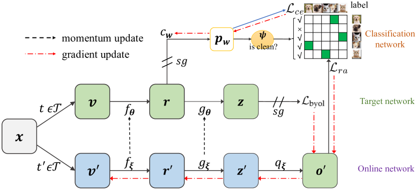
Fig. 1: Overall framework of our proposed method. Subscript $i$ is omitted here and sg is short for stopping gradient.

Let $\bm{x}_{i}$ be an image, $\bm{y}_{i}$ be its clean label, and $\bar{\bm{y}}_{i}$ be a noisy version of $\bm{y}_{i}$. A CNN usually has two parts [1, 2]: (i) Backbone $f$, which stacks multiple convolutional and pooling layers, and extracts the representation for input image $\bm{x}_{i}$ as $\bm{r}_{i}=f_{\bm{\theta}}(\bm{x}_{i})$. (ii) Classifier $c$, which is usually a linear projector with parameter $\bm{w}$ and produces predictions from the given representation as $c_{\bm{w}}(\bm{r}_{i})$. Thus, we denote a CNN as $C(\bm{x}_{i})=c_{\bm{w}}(f_{\bm{\theta}}(\bm{x}_{i}))$.

BYOL is composed of the bottom two parts in Figure 1, i.e., an online network and a target network. It first produces two augmented views $\bm{v}\!=\!t(\bm{x})$ and $\bm{v}^{\prime}\!=\!t^{\prime}(\bm{x})$ from $\bm{x}$ by applying twice random augmentation. The view $\bm{v}^{\prime}$ passes through an online network with the backbone $f_{\bm{\xi}}$, the projector $g_{\bm{\xi}}$ and the predictor ${q}_{\bm{\xi}}$ in turn to get features $\bm{r}^{\prime}$, $\bm{z}^{\prime}$ and $\bm{o}^{\prime}$ respectively. Another view $\bm{v}$ will be transformed to $\bm{r}$ and $\bm{z}$ by a similar target network, which has no prediction module. The target network’s parameters $\bm{\theta}$ are an exponential moving average of the online parameters $\bm{\xi}$, i.e., $\bm{\theta}=\tau\bm{\theta}+(1-\tau)\bm{\xi}$ with momentum rate $\tau\in\left[0,1\right]$. The training loss of BYOL is defined as a mean squared error:

$$\mathcal{L}_{\text{byol}}(\bm{x}_{i})=\left\|\bm{o}^{\prime}_{i}-\bm{z}_{i}\right\|^{2}_{2}.$$ (1)

2.2 Dealing with noisy label

2.2.1 Robust training of the classifier

To begin with, we add a linear classifier $c_{\bm{w}}$ on the top of the backbone $f_{\bm{\theta}}$ of target network (see Figure 1). Different from the standard supervised learning schema, we equip a $\mathsf{sg}$ (stop-gradient) operation between the backbone $f_{\bm{\theta}}$ and the classifier $c_{\bm{w}}$. Thus, we only use the gradients here to update the classifier. The objective for the classification branch is

$$\mathcal{L}_{\text{ce}}(\bm{x}_{i})=\mathsf{CE}\Big{(}c_{\bm{w}}\big{[}\mathsf{sg}\left(f_{\bm{\theta}}(t(\bm{x}_{i}))\right)\big{]},\bar{\bm{y}}_{i}\Big{)},$$ (2)

where $\mathsf{CE}(\cdot,\cdot)$ denotes the cross-entropy loss function and the training sample $(\bm{x}_{i},\bar{\bm{y}}_{i})$ is drawn from a noisy dataset.

The $\mathsf{sg}$ operator is very important here. We know that the classifier is more robust than the representation in presence of noisy labels, and the representation is inherent from the target network, which can capture some distinct patterns in images by SSRL. Thus, the gradients from $\mathcal{L}_{\text{ce}}$ can help train the classifier to predict correct labels, and the $\mathsf{sg}$ operator avoids the gradients from noisy labels affecting the representation. These will also been empirically shown in Section 3.3.

2.2.2 Identify clean labels

Next, since the classifier can predict correct labels, we can roughly separate the training samples into two groups, i.e., a group whose labels are likely to be correct (denote as $\mathsf{L}$) and another group whose labels are likely to be wrong (denote as $\mathsf{U}$). Inspired by [19, 25], we cluster samples based on their loss, as small loss samples are more likely to have clean labels. We use a two-components Gaussian mixture model (GMM) [26] $\psi$ to measure whether the sample is more likely to have clean label. In this way, the classification branch helps us find clean labels from the training samples.

2.2.3 Combine clean labels with SSRL

We know that once the labels are clean enough, we can use the clean labels to improve the representation learned by SSRL. Here, we introduce a representation alignment loss $\mathcal{L}_{\text{ra}}$, to assist the SSRL. Specifically, $\mathcal{L}_{\text{ra}}$ is defined as

$$\mathcal{L}_{\text{ra}}(\bm{x}_{i})\!=\!\sum\nolimits_{j=1}^{N_{L}}\mathbbm{1}_{j\neq i}\mathbbm{1}_{\bm{x}_{i},\bm{x}_{j}\in\mathsf{L}}\mathbbm{1}_{\bar{\bm{y}}_{i}=\bar{\bm{y}}_{j}}\left\|\bm{o}^{\prime}_{i}-\bm{z}_{i}\right\|^{2}_{2},$$ (3)

where $\mathbbm{1}_{\text{condition}}\!\in\!\{0,1\}$ is an indicator function evaluating $1$ iff condition is true, $N_{L}$ is the number of samples in $\mathsf{L}$. Different from (1) that treats two different augmented views from the same image $\bm{x}_{i}$ as a positive pair ($\bm{v}_{i}=t(\bm{x}_{i}),\bm{v}_{i}^{\prime}=t^{\prime}(\bm{x}_{i})$). (3) considers more positive pairs from different images but sharing the same label, and make sure that only clean labeled data (i.e., $\mathsf{L}$) can be used here to avoid bad effect of noise on representation learning.

2.3 Training details

Many state-of-the-art methods [25, 19, 27, 28] get excellent results with the help of image Mixup and model ensembling. Image Mixup is a simple learning technique proposed in [27], which trains a neural network on the combination of pairs of images and their labels. Model ensembling ensembles the model output of two separate neural networks to improve generalization. Due to their superiority and simple usage, we also use the two techniques to enhance CS³NL here.

Finally, the total training loss can be formulated as the combination of losses in (1), (2) and (3), i.e.,

$$\mathcal{L}=\sum\nolimits_{i=1}^{N}\mathcal{L}_{\text{byol}}(\bm{x}_{i})+\lambda_{1}\mathcal{L}_{\text{ra}}(\bm{x}_{i})+\lambda_{2}\mathcal{L}_{\text{ce}}(\bm{x}_{i}),$$ (4)

on the $N$ images $\bm{x}_{i}$ in the training set. $\lambda_{1}$ and $\lambda_{2}$ weight the importance between these three losses. In our experiments, we set $\lambda_{1}$ and $\lambda_{2}$ to 1. The model parameters are optimized by stochastic gradient descent with mini-batches of datasets.

3 Experiments

In this section, experiments are performed on three popular benchmark datasets [25]: CIFAR-10, CIFAR-100 [29] and WebVison [30]. All algorithms are implemented in PyTorch, and run on a linux server with 8 NVIDIA RTX 3090 GPUs.

3.1 Synthetic noisy labels

Following [19, 25], we add both symmetric and asymmetric noise on CIFAR-10, and only symmetric noise on CIFAR-100 with different levels of noises. The proposed CS³NL is compared with the following methods:

• Standard: directly trains the network with noisy labels;

• Mixup [27]: the image mixup technique on top of Standard.

• F-correction [16], Meta-Learn [31] and M-correction [17]: correct the training objects or select the clean samples to robustify training;

• Co-teaching [19]: trains two networks and each network selects clean samples for training the other, and its extensions DivideMix [25], ELR+ [32] AugDesc [33].

In particular, M-correction, DivideMix, ELR+, AugDesc are enhanced with the Mixup technique. Currently, ELR+ and AugDesc are the state-of-the-arts. Following  [25, 32], PreAct-ResNet18 is used as backbone for all the methods.

Table 1 shows the highest testing accuracies across training epochs. We observe that methods utilizing memorization effect in the third part are better then methods correcting the noisy labels in second parts. The mixup technique is beneficial when applied to different methods. DivideMix and ELR+ have comparable performance, showing the benefits of combining clean sample selection by two joint networks. AugDesc is better than other baselines. The proposed CS³NL outperforms all competing methods. The improvement is particularly significant on higher noise. For example, at the noise level of 90%, the relative improvement over the best baseline is 7.2% on CIFAR-10, and 18.6% on CIFAR-100. This demonstrate the significance of SSRL.

Table 1: Testing accuracies (%) on the CIFAR-10 and CIFAR-100 datasets. Results of the baselines are from [25, 32], where“-” means the corresponding result is not available. The highest accuracy is in bold.

	CIFAR-10					CIFAR-100
	sym noise				asym	sym noise
	20%	50%	80%	90%	40%	20%	50%	80%	90%
Standard	86.8	79.4	62.9	42.7	85.0	62.0	46.7	19.9	10.1
Mixup [27]	95.6	87.1	71.6	52.2	-	67.8	57.3	30.8	14.6
F-correction [16]	86.8	79.8	63.3	42.9	87.2	61.5	46.6	19.9	10.2
Meta-Learn [31]	92.9	89.3	77.4	58.7	89.2	68.5	59.2	42.4	19.5
M-correction [17]	94.0	92.0	86.8	69.1	87.4	73.9	66.1	48.2	24.3
Co-teaching [19]	89.5	85.7	67.4	47.9	-	65.6	51.8	27.9	13.7
DivideMix [25]	96.1	94.6	93.2	76.0	93.4	77.3	74.6	60.2	31.5
ELR+ [32]	95.8	94.8	93.3	78.7	93.0	77.6	73.6	60.8	33.4
AugDesc [33]	96.3	95.1	93.8	83.9	94.4	79.5	75.2	64.4	41.2
CS3NL	96.3	95.2	94.4	89.9	94.7	78.2	76.7	67.0	48.9

3.2 Real-world noisy labels

Following [18, 34], we only compare on the mini WebVision dataset [30], which contains the top 50 classes from the ImageNet ILSVRC12 subsets [7], and has about 66K noisy samples for training and 50K clean samples for validation.

As in [25, 32], we use the InceptionResNetV2 network as backbone and compare CS³NL with the following methods: F-correction [16], Co-teaching [19], DivideMix [25], and ELR+ [32]. Besides, we also compare with Iterative-CV [34], which identifies clean samples by cross-validation; MentorNet [18], which trains a student network on samples weighed by a pre-trained teacher network; D2L [35], which linearly combines label and model predictions. Following [25, 32], the models are evaluated with Top-1 and Top-5 prediction accuracies in Table 2. Again, DivideMix and ELR+ are very competitive in the real-word noisy labels, but the proposed method outperforms all consistently on both datasets.

Table 2: Comparison with baseline methods on WebVision and ILSVRC12. Results of others are copied from [25, 32].

	WebVision		ILSVRC12
	Top-1 (%)	Top-5 (%)	Top-1 (%)	Top-5 (%)
F-correction [16]	61.12	82.68	57.36	82.36
Co-teaching [19]	63.58	85.20	61.48	84.70
DivideMix [25]	77.32	91.64	75.20	90.84
ELR+ [32]	77.78	91.68	70.29	89.76
Iterative-CV [34]	65.24	85.34	61.60	84.98
MentorNet [18]	63.00	81.40	57.80	79.92
D2L [35]	62.68	84.00	57.80	81.36
CS3NL	79.12	93.00	77.20	93.04

3.3 Ablation studies

To evaluate the effectiveness of our novel refinements proposed in Section 2, we perform a serial of ablation studies for different training strategies (i.e., (i)-(v)) on the CIFAR10 dataset with ResNet34 as the backbone. Meanwhile, we keep the same hyperparameters setting as described in Section 3.1 for a fair comparison. Medium (40%) and high (80%) levels of symmetric noise are used, following [32]. Besides, to verify the upper bound performance of our proposed jointly training approach, we further perform experiments with a clean CIFAR10 dataset (i.e., 0%). To fully understand the significance of SSRL, a purely supervised learning baseline (vi)) is also included here. Six models are compared:

1. CS³NL: The proposed method.

2. Online CS³NL: Based on (i), instead of training classifier $c_{\bm{w}}$ on the top of backbone module from the target network, we choose the backbone module from the online network;

3. w/o $\mathsf{sg}$ in (2): Based on (i), we discard the stop-gradient operation in (2);

4. w/o $\psi$: Based on (i), we discard the label cleaning module $\psi$ and regard all training data as $\mathsf{L}$;

5. w/o (3): Based on (i), we exclude the SSRL loss in (3) from the total loss in (4);

6. Standard: we train a CNN in an end-to-end learning manner using the standard cross-entropy loss.

From Table 3, we observe that changing target network to online network has little influence as their parameters are shared. Stop gradient is the most important part here since it decouples the representation learning and classifier learning. In addition, all of the design components can improve the robustness against noisy label compared with standard setting.

Table 3: Validation experiments for evaluating the effectiveness of our novel refinements of CS³NL. The values in parentheses mean the absolute gap to CS³NL

	Setting	0%	40%	80%
(i)	CS3NL	96.9	94.6	88.1
(ii)	Online CS3NL	95.6 (-1.3)	94.1 (-0.5)	87.6 (-0.5)
(iii)	w/o $\mathsf{sg}$ in (2)	95.8 (-1.1)	91.4 (-3.2)	80.7 (-7.4)
(iv)	w/o $\psi$	95.7 (-1.2)	92.5 (-2.1)	86.2 (-1.9)
(v)	w/o (3)	94.3 (-2.6)	93.6 (-1.0)	87.9 (-0.2)
(vi)	Standard	96.8 (-0.1)	81.3 (-13.3)	62.9 (-25.2)

4 RELATION TO PRIOR WORKS

4.1 Noisy label learning

The methods studying the robustness of training CNNs with noisy labels can be categorized into three directions. The first type estimates a noisy transition matrix on the noisy labels [14, 15], but the transition matrix is hard to estimate correctly. The second type modifies or redesigns the training loss to improve the robustness [16, 17]. However, as the CNNs are often over-parameterized, the influence of noisy label still exists given sufficient training time [11]. The third type conducts label division based on the memorization effect, which tries to distinguishes the noise samples, discard or reuse them [9, 18, 19]. Different from these approaches, we explore CNN training mechanism with noisy labels from two perspectives, i.e., classifier learning and representation learning. And we combine SSRL and supervised learning with noisy labels to make both parts better.

4.2 Semi-supervised representation learning (SSRL)

SSRL [20, 21] is a kind of unsupervised learning method where no labels are required. Recently, SSRL achieves state-of-the-art performance in unsupervised training of neural networks by contrastive proxy task [22], which maximizes (resp. minimizes) the intra- (resp. inter-) class distances. In this work, we adopt the BYOL framework [24] which achieves remarkable performance. While SSRL can help learn better representations, it does not utilize any label information which can contain more meaningful visual semantics. By observing the learning behavior of representation learning and classifier learning as well as that of SSRL and supervised learning with noisy labels, we are the first to combine SSRL and supervised learning to enhance the CNN’s robustness to noisy labels. The new framework in Figure 1 has significant advance in the noisy label learning problem.

5 Conclusion

In this paper, we look deeply into the robustness of representation and classifier learning in the presence of noisy labels. We find that noisy labels will damage the representation learning significantly than classifier learning, and the classifier itself can exhibit strong robustness w.r.t. noisy labels with a good representation. Motivated by this, we proposed a robust CNN training manner to take care of both representation learning and classifier learning. By combining it with the current SOTA self-supervised representation learning framework, a large-scale improvement has been achieved.

References

- [1] Y. LeCun, L. Bottou, Y. Bengio, and P. Haffner, “Gradient-based learning applied to document recognition,” Proceedings of the IEEE, vol. 86, no. 11, pp. 2278–2324, 1998.
- [2] I. Goodfellow, Y. Bengio, and A. Courville, Deep learning, MIT press, 2016.
- [3] K. He, X. Zhang, S. Ren, and J. Sun, “Deep residual learning for image recognition,” in CVPR, 2016.
- [4] C. Szegedy, W. Liu, Y. Jia, et al., “Going deeper with convolutions,” in CVPR, 2015, pp. 1–9.
- [5] S. Ren, K. He, R. Girshick, and J. Sun, “Faster r-cnn: Towards real-time object detection with region proposal networks,” NeurIPS, vol. 28, 2015.
- [6] K. He, G. Gkioxari, P. Dollár, and R. Girshick, “Mask R-CNN,” in ICCV, 2017.
- [7] O. Russakovsky, J. Deng, H. Su, et al., “Imagenet large scale visual recognition challenge,” IJCV, vol. 115, pp. 211–252, 2015.
- [8] T. Lin, M. Maire, S. Belongie, et al., “Microsoft coco: Common objects in context,” in ECCV. Springer, 2014, pp. 740–755.
- [9] D. Arpit, S. Jastrzbski, N. Ballas, et al., “A closer look at memorization in deep networks,” in ICML. PMLR, 2017, pp. 233–242.
- [10] B. Neyshabur, S. Bhojanapalli, D. McAllester, and N. Srebro, “Exploring generalization in deep learning,” in NeurIPS, 2017.
- [11] C. Zhang, S. Bengio, M. Hardt, B. Recht, and O. Vinyals, “Understanding deep learning requires rethinking generalization,” in ICLR, 2017.
- [12] L. Jiang, D. Huang, M. Liu, and W. Yang, “Beyond synthetic noise: Deep learning on controlled noisy labels,” in ICML. PMLR, 2020, pp. 4804–4815.
- [13] B. Han, Q. Yao, T. Liu, G. Niu, I. W Tsang, J. T Kwok, and M. Sugiyama, “A survey of label-noise representation learning: Past, present and future,” Tech. Rep., arXiv:2011.04406, 2020.
- [14] S. Sukhbaatar, J. Bruna, M. Paluri, L. Bourdev, and R. Fergus, “Training convolutional networks with noisy labels,” in ICLR, 2015.
- [15] T. Xiao, T. Xia, Y. Yang, C. Huang, and X. Wang, “Learning from massive noisy labeled data for image classification,” in CVPR, 2015.
- [16] G. Patrini, A. Rozza, A. Krishna Menon, R. Nock, and L. Qu, “Making deep neural networks robust to label noise: A loss correction approach,” in CVPR, 2017.
- [17] E. Arazo, D. Ortego, P. Albert, N. O’Connor, and K. McGuinness, “Unsupervised label noise modeling and loss correction,” in ICML, 2019.
- [18] J. Lu, Z. Zhou, T. Leung, et al., “Mentornet: Learning data-driven curriculum for very deep neural networks on corrupted labels,” in ICML. PMLR, 2018, pp. 2304–2313.
- [19] B. Han, Q. Yao, X. Yu, G. Niu, M. Xu, W. Hu, I. Tsang, and M. Sugiyama, “Co-teaching: Robust training of deep neural networks with extremely noisy labels,” in NeurIPS, 2018.
- [20] T. Chen, S. Kornblith, M. Norouzi, and G. Hinton, “A simple framework for contrastive learning of visual representations,” in ICML, 2020.
- [21] K. He, H. Fan, Y. Wu, S. Xie, and R. Girshick, “Momentum contrast for unsupervised visual representation learning,” in CVPR, 2020.
- [22] K. Chaitanya, E. Erdil, N. Karani, and E. Konukoglu, “Contrastive learning of global and local features for medical image segmentation with limited annotations,” NeurIPS, vol. 33, pp. 12546–12558, 2020.
- [23] T. M Mitchell, Machine learning, vol. 1, McGraw-hill New York, 1997.
- [24] J. Grill, F. Strub, F. Altché, et al., “Bootstrap your own latent-a new approach to self-supervised learning,” NeurIPS, vol. 33, pp. 21271–21284, 2020.
- [25] J. Li, R. Socher, and S. Hoi, “Dividemix: Learning with noisy labels as semi-supervised learning,” in ICLR, 2020.
- [26] D. A Reynolds et al., “Gaussian mixture models.,” Encyclopedia of biometrics, vol. 741, no. 659-663, 2009.
- [27] H. Zhang, M. Cisse, Y. Dauphin, and D. Lopez-Paz, “MixUp: Beyond empirical risk minimization,” in ICLR, 2018.
- [28] J. Han, P. Luo, and X. Wang, “Deep self-learning from noisy labels,” in ICCV, 2019.
- [29] A. Krizhevsky, G. Hinton, et al., “Learning multiple layers of features from tiny images,” 2009.
- [30] W. Li, L. Wang, W. Li, E. Agustsson, and L. Van Gool, “Webvision database: Visual learning and understanding from web data,” Tech. Rep., 2017.
- [31] J. Li, Y. Wong, Q. Zhao, and M. S Kankanhalli, “Learning to learn from noisy labeled data,” in CVPR, 2019, pp. 5051–5059.
- [32] S. Liu, J. Niles-Weed, N. Razavian, and C. Fernandez-Granda, “Early-learning regularization prevents memorization of noisy labels,” NeurIPS, vol. 33, pp. 20331–20342, 2020.
- [33] K. Nishi, Y. Ding, A. Rich, and T. Hollerer, “Augmentation strategies for learning with noisy labels,” in CVPR, 2021, pp. 8022–8031.
- [34] P. Chen, B. Liao, G. Chen, and S. Zhang, “Understanding and utilizing deep neural networks trained with noisy labels,” in ICML, 2019.
- [35] X. Ma, Y. Wang, M. E Houle, et al., “Dimensionality-driven learning with noisy labels,” in ICML, 2018.