Complex Langevin Dynamics and Supersymmetric Quantum Mechanics

Abstract

Using complex Langevin method we probe the possibility of dynamical supersymmetry breaking in supersymmetric quantum mechanics models with complex actions. The models we consider are invariant under the combined operation of parity and time reversal, in addition to supersymmetry. When actions are complex traditional Monte Carlo methods based on importance sampling fail. Models with dynamically broken supersymmetry can exhibit sign problem due to the vanishing of the partition function. Complex Langevin method can successfully evade the sign problem. Our simulations suggest that complex Langevin method can reliably predict the absence or presence of dynamical supersymmetry breaking in these one-dimensional models with complex actions.

1 Introduction

The phenomenon of spontaneous breaking of supersymmetry (SUSY) requires an understanding of non-perturbative aspects of quantum field theory Witten:1981nf ; Witten:1982df . Lattice regularized form of the field theory path integral provides a systematic tool to investigate numerous non-perturbative features of quantum field theories. Monte Carlo methods have been used to reliably extract the physics of such systems. The basic idea behind path integral Monte Carlo is to generate field configurations with a positive definite probability weight, given by the exponential of the negative of the action (in Euclidean spacetime), and then compute the path integral by statistically averaging these importance sampled ensemble of field configurations. However, when the action is complex, for example, when studying QCD at finite temperature and baryon/quark chemical potential, QCD with a theta term, Chern-Simons gauge theories, or chiral gauge theories, the fermion determinant of the theory can be complex, and this feature results in the so-called sign problem. This makes the simulation algorithms based on path integral Monte Carlo unreliable.

There exist very few methods in the literature that can effectively handle or evade this infamous sign problem. Some of these include methods such as analytical continuation, Taylor series expansion deForcrand:2002hgr , methods based on the complexification of the integration variables such as the Lefschetz thimble method PhysRevD.86.0745006 and the complex Langevin (CL) method Klauder:1983nn ; Klauder:1983zm ; Klauder:1983sp ; Parisi:1984cs ; Damgaard:1987rr . (See Refs. Cristoforetti:2012su ; Fujii:2013sra ; DiRenzo:2015foa ; Tanizaki:2015rda ; Fujii:2015vha ; Alexandru:2015xva for simulations based on the Lefschetz thimble method.) The CL method is based on stochastic quantization, and it is a straightforward generalization of the real Langevin method into complexified field configurations.

The central theme of stochastic quantization is that the expectation values of observables are obtained as the equilibrium values of a stochastic process. In Langevin dynamics, this is achieved by evolving the system in a fictitious time direction $\theta$ (Langevin time) subject to Gaussian stochastic noise. The idea of stochastic quantization for ordinary field theory systems with real actions is extended to the cases with complex actions, and this overcomes the sign problem by defining a stochastic process, with complexified field variables, using Langevin equations for the complex action Klauder:1985kq ; Klauder:1985ks ; Gausterer:1986gk . The use of Langevin equations, rather than importance sampling, waives the restriction of real and positive semi-definite measures. Such a strategy makes the real field variables $\phi$ complex, during the Langevin evolution, since the gradient of the action, the drift term, becomes complex.

The complex Langevin equation in Euler discretized form for the field variable $\phi$ reads

$$\phi(\theta+\epsilon)=\phi(\theta)-\left[\frac{\delta S[\phi]}{\delta\phi(\theta)}\right]\epsilon+\eta(\theta)\sqrt{\epsilon},$$ (1.1)

where $S[\phi]$ is the action of the theory, the Langevin time is discretized as an integer multiple of the Langevin step size $\epsilon$, and $\eta(\theta)$ is a Gaussian noise satisfying the constraints $\langle\eta(\theta)\rangle=0$ and $\langle\eta(\theta)\eta(\theta^{\prime})\rangle=2\delta_{\theta\theta^{\prime}}$. In our simulations, we use real Gaussian stochastic noise to control excursions in the imaginary directions of the field configurations Aarts:2011ax .

Noise averaged expectation value for an arbitrary operator ${\cal O}[\phi]$ can be defined as

$$\left\langle{\cal O}[\phi(\theta)]\right\rangle_{\eta}=\int d\phi P[\phi(\theta)]{\cal O}[\phi],$$ (1.2)

where the probability distribution $P[\phi(\theta)]$ satisfies the Fokker-Planck equation

$$\frac{\partial P[\phi(\theta)]}{\partial\theta}=\frac{\delta}{\delta\phi(\theta)}\left[\frac{\delta}{\delta\phi(\theta)}+\frac{\delta S[\phi]}{\delta\phi(\theta)}\right]P[\phi(\theta)].$$ (1.3)

In the case of real action it can be easily shown that in the large Langevin time limit, $\theta\to\infty$, the stationary solution of the Fokker-Planck equation

$$P[\phi]\sim\exp\left(-S[\phi]\right)$$ (1.4)

will be reached, and thus ensuring the convergence of the Langevin dynamics to the correct equilibrium distribution. When the action is complex, the situation is challenging. The field configurations are complexified due to the drift term being a complex quantity and thus, we end up with complex probabilities. The CL method became very popular when it was first proposed in the 1980s, but certain problems were encountered shortly after. First was the problem of runaways, where the field configurations would not converge, and the second was the convergence to a wrong limit. In recent years, the CL method has been successfully revived, producing correct results even when the sign problem is severe. When applying the CL method, it is essential that the expectation values computed with a real probability $P[\phi]$ along the complex trajectory $\phi=x+iy$ are in agreement with the original expectation values with complex weight $\rho(\phi)=e^{-S(\phi)}$. That is,

$$\left\langle{\cal O}\right\rangle=\int dxdyP[x,y]{\cal O}[x+iy]=\int d\phi\rho[\phi]{\cal O}[\phi].$$ (1.5)

Recently, the proof towards convergence to the complex weight in the above equivalence has been an object of thorough study, and correctness criteria have been proposed for the validity of the method Aarts:2009uq ; Nagata:2015uga . In Appendix. A, we discuss these criteria and investigate the reliability of the simulations carried out in this work. The revived interest in this field has led to promising developments in the optimization of the method. It has been noted that the complexification of field variables can drastically influence the Langevin trajectory, making large excursions in the imaginary direction. For instance, it might get closer to unstable directions. An efficient algorithm to evade such a situation involves considering adaptive Langevin step size in the numerical integration of Langevin equations Aarts:2009dg . Ref. Damgaard:1987rr provides a pedagogical review on this method, and Ref. Berger:2019odf is a recent review in the context of the sign problem in quantum many-body physics.

The CL method has been used successfully in the study of various models in the recent past Berges:2005yt ; Berges:2006xc ; Berges:2007nr ; Bloch:2017sex ; Aarts:2008rr ; Pehlevan:2007eq ; Aarts:2008wh ; Aarts:2009hn ; Aarts:2010gr ; Aarts:2011zn . There have also been studies of spontaneous symmetry breaking (SSB) induced by complex fermion determinant Ito:2016efb ; Ito:2016hlj ; Anagnostopoulos:2017gos and a recent study addressing the SSB of $SO(D)$ rotational symmetry based on CL method Anagnostopoulos:2020xai . In Ref. Basu:2018dtm the authors used CL simulations to observe the Gross-Witten-Wadia (GWW) Gross:1980he ; Wadia:2012fr ; Wadia:1980cp phase transition in certain large-$N$ matrix models. In Ref. Joseph:2019sof the authors looked at certain classes of zero-dimensional supersymmetric quantum field theories with complex actions using the CL method. In this work we will investigate dynamical SUSY breaking in an interesting class of supersymmetric actions that are complex and exhibiting invariance under the combine operation of parity and time reversal (${\cal PT}$) symmetry. This class of actions cannot be studied using traditional Monte Carlo methods.

The paper is organized as follows. In Sec. 2 we briefly introduce supersymmetric quantum mechanics with two supercharges. In Sec. 3 we discuss the lattice regularization of the model. There, we also provide a set of useful observables that can probe SUSY breaking in the system. They include correlation functions and Ward identities. In Sec. 4 we present the simulation results of various models including the ${\cal PT}$ symmetric model. Conclusions are provided in Sec. 5. In Appendix A.1 we study the reliability of simulations using the Langevin operator and in Appendix A.2 we examine the correctness of simulations by observing the fall-off behavior of the probability distributions of the drift term magnitudes.

2 Supersymmetric quantum mechanics

Let us consider the action $S[\phi,\psi,{\overline{\psi}}]$ of a supersymmetric quantum mechanics with a general superpotential $W(\phi)$. The model is invariant under two supercharges. The degrees of freedom are a scalar field $\phi$ and two fermions $\psi$ and ${\overline{\psi}}$. We take the action to be an integral over a compactified time circle of circumference $\beta$ in Euclidean time. It has the form

$$S[\phi,\psi,{\overline{\psi}}] = \int_{0}^{\beta}d\tau\Bigg{[}\frac{1}{2}{\mathcal{B}}(\tau)^{2}+i{\mathcal{B}}\left(\frac{\partial}{\partial{\tau}}{\phi(\tau)}+\frac{\partial}{\partial{\phi}}W(\phi(\tau))\right)$$ (2.1)

$$\hskip 56.9055pt+{{\overline{\psi}}(\tau)}\left(\frac{\partial}{\partial{\tau}}+\frac{\partial^{2}}{\partial{\phi}^{2}}{W}(\phi(\tau))\right)\psi(\tau)\Bigg{]},$$

where ${\mathcal{B}}$ is an auxiliary field and the derivatives with respect to $\tau$ and $\phi$ are denoted by a dot and a prime, respectively.

Denoting the two supercharges by ${\mathcal{Q}}$ and ${\overline{\mathcal{Q}}}$, the SUSY transformations have the form

$${\mathcal{Q}}\phi=\psi,~{}~{}~{}{\mathcal{Q}}\psi=0,~{}~{}~{}{\mathcal{Q}}{\overline{\psi}}=-i{\mathcal{B}},~{}~{}~{}{\mathcal{Q}}{\mathcal{B}}=0,$$ (2.2)

and

$${\overline{\mathcal{Q}}}\phi=-{\overline{\psi}},~{}~{}~{}{\overline{\mathcal{Q}}}\bar{\psi}=0,~{}~{}~{}{\overline{\mathcal{Q}}}\psi=-i{\mathcal{B}}+2\dot{\phi},~{}~{}~{}{\overline{\mathcal{Q}}}{\mathcal{B}}=2i\dot{{\overline{\psi}}}.$$ (2.3)

The supercharges satisfy the algebra

$$\{{\mathcal{Q}},{\mathcal{Q}}\}=0,\quad\{{\overline{\mathcal{Q}}},{\overline{\mathcal{Q}}}\}=0,\quad\{{\mathcal{Q}},{\overline{\mathcal{Q}}}\}=2\partial_{\tau}.$$ (2.4)

We also note that the action can be expressed in ${\mathcal{Q}}$- and ${\mathcal{Q}}{\overline{\mathcal{Q}}}$-exact forms. That is,

$$S={\mathcal{Q}}\int_{0}^{\beta}d{\tau}~{}{\overline{\psi}}\left[\frac{i}{2}{\mathcal{B}}-\left(\frac{\partial\phi}{\partial\tau}+W^{{}^{\prime}}(\phi)\right)\right]={\mathcal{Q}}{\overline{\mathcal{Q}}}\int_{0}^{\beta}d\tau\left(\frac{1}{2}{\overline{\psi}}\psi+W(\phi)\right).$$ (2.5)

The partition function in path integral formalism is defined by

$$Z\equiv\int{\cal D}{\mathcal{B}}{\cal D}\phi{\cal D}\psi{\cal D}{\overline{\psi}}~{}e^{-S[\phi,\psi,{\overline{\psi}}]}$$ (2.6)

with periodic temporal boundary conditions for all the fields.

In a system with unbroken SUSY, we can consider a Hamiltonian $H$ corresponding to the Lagrangian in Eq. (2.1) having energy levels $E_{n}$ where $n=0,1,2,\dots$, such that the ground state energy $E_{0}=0$. Then, the bosonic and fermionic excited states form a SUSY multiplet

$$|b_{n+1}\rangle=\frac{1}{\sqrt{2E_{n+1}}}{\overline{\mathcal{Q}}}|f_{n}\rangle,~{}~{}~{}|f_{n}\rangle=\frac{1}{\sqrt{2E_{n+1}}}{\mathcal{Q}}|b_{n+1}\rangle$$ (2.7)

satisfying the algebra given in Eq. (2.4), with $|b_{0}\rangle$ being the ground state of the system. Assuming that the states $|b_{n}\rangle$ and $|f_{n}\rangle$ have the fermion number charges $F=0$ and $F=1$, respectively, when periodic temporal boundary conditions are imposed for both the bosonic and fermionic fields, $Z$ is equivalent to the Witten index $\Delta_{W}\left(\beta\right)$ Witten:1982df . It is easy to see that the partition function defined as

$$Z=\Delta_{W}\left(\beta\right)={\rm Tr~{}}\left[(-1)^{F}e^{-\beta H}\right]=\langle b_{0}|b_{0}\rangle+\sum_{n=0}^{\infty}\left[\left(\langle b_{n+1}|b_{n+1}\rangle-\langle f_{n}|f_{n}\rangle\right)e^{-\beta E_{n+1}}\right]$$ (2.8)

does not vanish due to the existence of a normalizable ground state. As a result, the normalized expectation values of observables are well-defined.

The normalized expectation value of the auxiliary field defined as

$$\langle{\mathcal{B}}\rangle=\frac{1}{\Delta_{W}\left(\beta\right)}\left[\langle b_{0}|{\mathcal{B}}|b_{0}\rangle+\sum_{n=0}^{\infty}\left(\langle b_{n+1}|{\mathcal{B}}|b_{n+1}\rangle-\langle f_{n}|{\mathcal{B}}|f_{n}\rangle\right)e^{-\beta E_{n+1}}\right]$$ (2.9)

can be used as an order parameter to probe SUSY breaking Kuroki:2009yg . (We note that the unpaired state appearing in Eqs. (2.8) and (2.9) need not have to be a bosonic state or a unique state.) The auxiliary field was introduced for the off-shell completion of the SUSY algebra. The ${\mathcal{Q}}$ transformation of ${\mathcal{B}}$ in Eq. (2.2) and the fact that the ground state is annihilated by the supercharges together imply that in the absence of SUSY breaking the normalized expectation value of the auxiliary field vanishes. However, in the SUSY broken case, we end up in a not-so-trivial situation.

In a system with SUSY spontaneously broken, the Hamiltonian $H$ corresponding to the Lagrangian in Eq. (2.1) has a positive ground state energy ($0<E_{0}<E_{1}<E_{2}\dots$), and the SUSY multiplet is defined as

$$|b_{n}\rangle=\frac{1}{\sqrt{2E_{n}}}{\overline{\mathcal{Q}}}|f_{n}\rangle,~{}~{}~{}|f_{n}\rangle=\frac{1}{\sqrt{2E_{n}}}{\mathcal{Q}}|b_{n}\rangle,$$ (2.10)

satisfying the algebra given in Eq. (2.4). Differently from the unbroken SUSY case, when SUSY is broken, the supersymmetric partition function

$$Z=\Delta_{W}={\rm Tr~{}}\left[(-1)^{F}e^{-\beta H}\right]=\sum_{n=0}^{\infty}\left[\left(\langle b_{n}|b_{n}\rangle-\langle f_{n}|f_{n}\rangle\right)e^{-\beta E_{n}}\right]$$ (2.11)

vanishes due to the cancellation between bosonic and fermionic states. As a consequence, the normalized expectation values of observables will be ill-defined. We consider the auxiliary field as an observable, and the normalized expectation value can be computed as

$$\langle{\mathcal{B}}\rangle=\frac{1}{\Delta_{W}\left(\beta\right)}\sum_{n=0}^{\infty}\left[\left(\langle b_{n}|{\mathcal{B}}|b_{n}\rangle-\langle f_{n}|{\mathcal{B}}|f_{n}\rangle\right)e^{-\beta E_{n}}\right],$$ (2.12)

where the numerator vanishes from ${\mathcal{Q}}$-supersymmetry $\left(\langle b_{n}|{\mathcal{B}}|b_{n}\rangle=\langle f_{n}|{\mathcal{B}}|f_{n}\rangle\right)$. Thus, in a system with broken SUSY, the normalized expectation of auxiliary field admit a $0/0$ indefinite form.

In Ref. Kuroki:2009yg Kuroki and Sugino introduced a regulator that explicitly breaks SUSY and resolves the degeneracy by fixing a single vacuum state in which SUSY is broken. This regulator $\alpha$ (the twist parameter) can be implemented by imposing twisted boundary conditions (TBC) for fermions. That is,

$$\psi(\tau+\beta)=e^{i\alpha}\psi(\tau)\quad{\rm and}\quad{\overline{\psi}}(\tau+\beta)=e^{-i\alpha}{\overline{\psi}}(\tau).$$ (2.13)

It was shown in Ref. Kuroki:2009yg that for a non-zero $\alpha$, the partition function does not vanish, and the normalized expectation value of the auxiliary field is well-defined. In the limit $\alpha\to 0$, PBCs are recovered and supersymmetry is restored. Thus $\alpha$ regularizes the indefinite form in Eq. (2.12). Now, vanishing expectation value of the auxiliary field in the limit $\alpha\to 0$ suggests that SUSY is not broken, while a non-zero value suggests that SUSY is broken. We incorporate the twist $\alpha$ when we introduce the lattice regularized theory in Sec. 3.1.

It is possible to integrate out the auxiliary field using its equation of motion

$${\mathcal{B}}=-i\left(\frac{\partial\phi}{\partial\tau}+W^{{}^{\prime}}(\phi)\right),$$ (2.14)

to get the on-shell form of the action

$$S=\int_{0}^{\beta}d\tau\left[\frac{1}{2}\left\{{\left(\frac{\partial\phi}{\partial\tau}\right)}+W^{{}^{\prime}}(\phi)\right\}^{2}+{{\overline{\psi}}}\left\{\frac{\partial}{\partial\tau}+W^{\prime\prime}(\phi)\right\}\psi\right].$$ (2.15)

Upon using the Leibniz integral rule and discarding the resultant total derivative term, the action takes the form

$$S=\int_{0}^{\beta}d\tau\left[\frac{1}{2}\left\{{\left(\frac{\partial\phi}{\partial\tau}\right)}^{2}+\left[W^{\prime}(\phi)\right]^{2}\right\}+{{\overline{\psi}}}\left\{\frac{\partial}{\partial\tau}+W^{\prime\prime}(\phi)\right\}\psi\right].$$ (2.16)

In the above expression, the total derivative term we omitted was $(\partial\phi/\partial\tau)W^{\prime}(\phi)$. Note that such an omission is only possible in the continuum theory. When we discretize the theory on a lattice, this term does not vanish, and its presence is crucial to ensure the ${\mathcal{Q}}$-exact lattice supersymmetry. Thus, in our lattice analysis, we will use Eq. (2.15) as the continuum target theory.

3 Lattice regularized models

We discretize the action given in Eq. (2.15) on a one-dimensional lattice. Let us take the lattice to be $\Lambda$, having $T$ number of equally spaced sites with lattice spacing $a$. The integral and continuum derivatives are replaced by a Riemann sum $a{\Sigma}$ and a lattice difference operator $\nabla$, respectively. The physical extent of the lattice is defined as $\beta\equiv Ta$.

There are several ways to regularize a given theory on a lattice. We will choose the prescription in which the derivatives appearing in the action take the form of a symmetric difference operator

$$\nabla^{S}_{ij}=\frac{1}{2}\left(\nabla^{+}_{ij}+\nabla^{-}_{ij}\right),$$ (3.1)

where

$$\nabla^{+}_{ij}=\frac{1}{a}(\delta_{i+1,j}-\delta_{i,j})\quad\longrightarrow\quad\nabla^{+}_{ij}f_{j}=\frac{1}{a}(f_{i+1}-f_{i}),{\rm~{}and}$$ (3.2)

$$\nabla^{-}_{ij}=\frac{1}{a}(\delta_{i,j}-\delta_{i-1,j})\quad\longrightarrow\quad\nabla^{-}_{ij}f_{j}=\frac{1}{a}(f_{i}-f_{i-1}),$$ (3.3)

are the forward and backward difference operators, respectively, and $i,j$ represent lattice sites. However, it is known that the symmetric derivative leads to the so-called fermion doubling problem and this, in turn, leads to a non-supersymmetric lattice theory. We can use the Wilson discretization prescription to decouple these extra fermionic modes from the system. The difference operator is modified as

$$\nabla^{W}_{ij}(r)=\nabla^{S}_{ij}-\frac{ra}{2}\square_{ij},$$ (3.4)

where $\square_{ij}=\nabla^{+}_{ik}\nabla^{-}_{kj}$ is the usual lattice Laplacian and the Wilson parameter $r\in\left[-1,1\right]/\left\{0\right\}$ Baumgartner:2014nka . For one-dimensional derivatives it turns out that the standard choice of $r=\pm 1$ yields $\nabla^{W}_{ij}(\pm 1)=\nabla^{\mp}_{ij}$, thereby suggesting that the doubling problem can be resolved by simply using forward or backward difference operator. The reason being that for any choice of the lattice difference operator, the theories can be made manifestly supersymmetric upon the addition of appropriate improvement terms corresponding to the discretization of continuum surface integrals Bergner:2007pu .

In our analysis, for the standard choice of the Wilson parameter, we follow the symmetric derivative with a Wilson mass matrix suggested in Ref. Catterall:2000rv . The lattice regularized action then takes the form

$$\mathcal{S}=a\sum_{i=0}^{T-1}\left[\frac{1}{2}\left(\sum_{j=0}^{T-1}\nabla^{S}_{ij}\phi_{j}+\Omega^{\prime}_{i}\right)^{2}+{\overline{\psi}}_{i}\sum_{j=0}^{T-1}\left(\nabla^{S}_{ij}+\Omega^{\prime\prime}_{ij}\right)\psi_{j}\right],$$ (3.5)

where the quantity $\Omega^{\prime}_{i}$ is defined as

$$\Omega^{\prime}_{i}=\sum_{j=0}^{T-1}K_{ij}\phi_{j}+W^{\prime}_{i},$$ (3.6)

and its derivative $\Omega^{\prime\prime}_{ij}$ is $\Omega^{\prime\prime}_{ij}=K_{ij}+W^{\prime\prime}_{ij}\delta_{ij}$. The Wilson mass matrix $K_{ij}$ has the form $K_{ij}=m\delta_{ij}-\frac{ra}{2}\square_{ij}$.

We can make the variables dimensionless by performing appropriate rescaling. Let us consider the following set of redefinitions for the variables

$$\widetilde{\phi}=a^{-1/2}\phi,\quad\widetilde{\nabla}^{S}=a\nabla^{S},\quad\widetilde{\Omega}^{\prime}=\sqrt{a}\Omega^{\prime},\quad\widetilde{\Omega}^{\prime\prime}=a\Omega^{\prime\prime}.$$ (3.7)

Under these rescalings the action becomes

$$\widetilde{\mathcal{S}}=\sum_{i=0}^{T-1}\left[\frac{1}{2}\left(\sum_{j=0}^{T-1}\widetilde{\nabla}^{S}_{ij}\widetilde{\phi}_{j}+\widetilde{\Omega}^{\prime}_{i}\right)^{2}+{\overline{\psi}}_{i}\sum_{j=0}^{T-1}\left(\widetilde{\nabla}^{S}_{ij}+\widetilde{\Omega}^{\prime\prime}_{ij}\right)\psi_{j}\right].$$ (3.8)

3.1 Theory on a lattice

For convenience, we will not be using the tilde sign on the dimensionless variables; all variables and fields mentioned from now on are understood to be dimensionless. Physical quantities will be labeled differently.

The supersymmetry transformations are modified to contain the Wilson mass terms. For a given lattice site $k$ they are given by

$${\mathcal{Q}}\phi_{k}=\psi_{k},\quad{\mathcal{Q}}{\overline{\psi}}_{k}=-N_{k},\quad{\mathcal{Q}}\psi_{k}=0,$$ (3.9)

and

$${\overline{\mathcal{Q}}}\phi_{k}=-{\overline{\psi}}_{k},\quad{\overline{\mathcal{Q}}}\psi_{k}=\overline{N}_{k},\quad{\overline{\mathcal{Q}}}\hskip 1.42271pt{\overline{\psi}}_{k}=0,$$ (3.10)

where

$$N_{k}=\nabla^{S}{\phi}_{k}+\Omega^{\prime}_{k},\quad{\rm and}\quad\overline{N}_{k}=\nabla^{S}{\phi}_{k}-\Omega^{\prime}_{k}.$$ (3.11)

The supercharges satisfy the algebra

$$\{{\mathcal{Q}},{\mathcal{Q}}\}=0,\quad\{{\overline{\mathcal{Q}}},{\overline{\mathcal{Q}}}\}=0,\quad{\rm and}\quad\{{\mathcal{Q}},{\overline{\mathcal{Q}}}\}=2\nabla^{S}.$$ (3.12)

The main obstacle that prevents the preservation of exact lattice SUSY is the failure of the Leibniz rule for lattice derivatives. Unlike the continuum action given in Eq. (2.15), the lattice regularized action

$$\mathcal{S}=\sum_{i=0}^{T-1}\left[\frac{1}{2}\left(\sum_{j=0}^{T-1}\nabla^{S}_{ij}\phi_{j}+\Omega^{\prime}_{i}\right)^{2}+{\overline{\psi}}_{i}\sum_{j=0}^{T-1}\left(\nabla^{S}_{ij}+\Omega^{\prime\prime}_{ij}\right)\psi_{j}\right]$$ (3.13)

preserves only the ${\mathcal{Q}}$ supercharge. The ${\overline{\mathcal{Q}}}$ supersymmetry is broken for $T\geq 2$. It can also be shown that the action is only ${\mathcal{Q}}$ invariant. That is, ${\mathcal{Q}}\mathcal{S}=0\neq{\overline{\mathcal{Q}}}\mathcal{S}$.

The ${\overline{\mathcal{Q}}}$ supersymmetry is broken for finite lattice size $T$ because it is not possible to define a corresponding ${\overline{\mathcal{Q}}}$ invariant transformation on lattice variables such that the algebra $\{{\mathcal{Q}},{\overline{\mathcal{Q}}}\}=2\nabla^{S}$ still holds Kanamori:2007yx . However, the ${\mathcal{Q}}$-exactness is essential and sufficient to kill any SUSY breaking counter-terms and thereby suppress lattice artifacts. See Refs. Catterall:2000rv ; Catterall:2003wd ; Giedt:2004vb ; Kuroki:2009yg for more discussions on this.

As mentioned in Sec. 2 for the continuum theory, when SUSY is broken, the partition function vanishes. In that case, the expectation values of the observables normalized by the partition function could be ill-defined. To overcome this difficulty in our lattice regularized theory, we will apply periodic boundary conditions for bosons and twisted boundary conditions for fermions Kuroki:2009yg ; Kuroki:2010au .

Introducing the twist, we have $\phi_{T}=\phi_{0},\quad\psi_{T}=e^{i\alpha}\psi_{0},\quad{\overline{\psi}}_{T}=e^{-i\alpha}{\overline{\psi}}_{0}$. For the case of dynamically broken SUSY, when $\alpha=0$, the Witten index vanishes, which dictates that the fermion determinant changes its sign depending on the boson field configurations. This is the sign problem in models with dynamical SUSY breaking.

The partition function given in Eq. (2.6) takes the following form

$$Z_{\alpha}=\left(\frac{1}{\sqrt{2\pi}}\right)^{T}\int\left(\prod_{k=0}^{T-1}d\phi_{k}d\psi_{k}d{\overline{\psi}}_{k}\right)e^{-\mathcal{S}_{\alpha}},$$ (3.14)

where $\mathcal{S}_{\alpha}$ is the lattice regularized action that respects the twisted boundary conditions.

We have

$$\mathcal{S}_{\alpha}=\sum_{i=0}^{T-1}\frac{1}{2}\bigg{(}\phi_{i}-\phi_{i-1}+m\phi_{i}+W^{\prime}_{i}\bigg{)}^{2}+\sum_{i=0}^{T-1}{\overline{\psi}}_{i}\bigg{(}\psi_{i}-\psi_{i-1}+\left(m+W^{\prime\prime}_{ii}\right)\psi_{i}\bigg{)}.$$ (3.15)

Let us absorb the mass term into the potential $W$, and define a new potential $\Xi$ as

$$\Xi\equiv\frac{1}{2}m\phi^{2}+W.$$ (3.16)

The action with twisted boundary conditions now takes the form

$$\mathcal{S}_{\alpha} = \sum_{i=0}^{T-1}\frac{1}{2}\bigg{(}\sum_{j=0}^{T-1}\nabla^{-}_{ij}\phi_{j}+\Xi^{\prime}_{i}\bigg{)}^{2}+\sum_{i=0}^{T-1}{\overline{\psi}}_{i}\bigg{(}\sum_{j=0}^{T-1}\nabla^{-}_{ij}+\Xi^{{}^{\prime\prime}}_{ij}\bigg{)}\psi_{j}.$$ (3.17)

Also the expressions for $N_{i}$ and $\overline{N}_{i}$ become

$$N_{i}=\sum_{j=0}^{T-1}\nabla^{S}_{ij}\phi_{j}+\Omega^{\prime}_{i}=\sum_{j=0}^{T-1}\nabla^{-}_{ij}\phi_{j}+\Xi^{\prime}_{i},$$ (3.18)

$$\overline{N}_{i}=\sum_{j=0}^{T-1}\nabla^{S}_{ij}\phi_{j}-\Omega^{\prime}_{i}=\sum_{j=0}^{T-1}\nabla^{+}_{ij}\phi_{j}-\Xi^{\prime}_{i}.$$ (3.19)

After integrating out fermions, the fermionic contribution to the partition function given in Eq. (3.14) has the form

$$Z_{\alpha}^{F} = \prod_{k=0}^{T-1}\left(1+\Xi^{{}^{\prime\prime}}_{kk}\right)-e^{i\alpha}.$$ (3.20)

This is nothing but the determinant of the twisted Wilson fermion matrix $\mathcal{W}_{\alpha}^{F}$

$$Z_{\alpha}^{F}=\det\left[\mathcal{W}_{\alpha}^{F}\right].$$ (3.21)

For periodic boundary conditions ($\alpha=0$ case) this is in agreement with the expression obtained in Ref. Catterall:2000rv .

The full partition function takes the form

$$Z_{\alpha}=\left(\frac{1}{\sqrt{2\pi}}\right)^{T}\int\left(\prod_{k=0}^{T-1}d\phi_{k}\right)~{}\exp\left[-\mathcal{S}^{\rm~{}eff}_{\alpha}\right],$$ (3.22)

with

$${\mathcal{S}_{\alpha}}^{\text{eff}} = {\mathcal{S}}^{B}-\ln\left({\rm det}\left[\mathcal{W}_{\alpha}^{F}\right]\right)$$ (3.23)

$$= \sum_{k=0}^{T-1}\frac{1}{2}\bigg{(}\phi_{k}-\phi_{k-1}+\Xi^{\prime}_{k}\bigg{)}^{2}-\ln\left(\prod_{k=0}^{T-1}\left(1+\Xi^{{}^{\prime\prime}}_{kk}\right)-e^{i\alpha}\right).$$

Given an observable $\mathcal{O}$, we can compute its expectation value as

$$\langle\mathcal{O}\rangle = \lim_{\alpha\to 0}\langle\mathcal{O}\rangle_{\alpha}$$ (3.24)

$$= \lim_{\alpha\to 0}\frac{1}{Z_{\alpha}}\left(\frac{1}{\sqrt{2\pi}}\right)^{T}\int\left(\prod_{k=0}^{T-1}d\phi_{k}\right)\mathcal{O}~{}\exp\left[{-\mathcal{S}_{\alpha}^{\text{eff}}}\right].$$

Note that the gradient of the action has to be computed to update the field configurations in the CL method. The drift term, given by the negative of the gradient of the action, contains the fermion determinant in the denominator, whose zeroes in the complexified space cause the subtlety for the conditions required for the justification of CL method. The dynamical variables may come close to the singularity of the drift term (the singular drift problem). A recent study highlighted that such a problem is not restricted to logarithmic singularities but is rather generic and may arise where the stochastic process involves a singular drift term Nishimura:2015pba .

3.2 Correlation functions

Using the expression given in Eq. (3.24) we can compute the correlation functions. The bosonic and fermionic correlation functions are defined as

$$G^{B}_{\alpha}(k)\equiv\langle\phi_{0}\phi_{k}\rangle_{\alpha}$$ (3.25)

and

$$G^{F}_{\alpha}(k)\equiv\langle{\overline{\psi}}_{0}\psi_{k}\rangle_{\alpha},$$ (3.26)

respectively, at the site $k$.

The fermionic correlation function can be shown to be

$$\langle{\overline{\psi}}_{0}\psi_{k}\rangle_{\alpha}=\frac{1}{Z_{\alpha}}\left(\frac{1}{\sqrt{2\pi}}\right)^{T}\int\left(\prod_{i=0}^{T-1}d\phi_{i}\right)\underbrace{\left(-\frac{{\langle{\overline{\psi}}_{0}\psi_{k}\rangle^{F}}}{\det\left[\mathcal{W}_{\alpha}^{F}\right]}\right)}_{\left[{\overline{\psi}}_{0}\psi_{k}\right]^{L}_{\alpha}}~{}\exp\left[-{S_{\alpha}}^{\text{eff}}\right].$$ (3.27)

Upon comparison with Eq. (3.24) we define $\left[{\overline{\psi}}_{0}\psi_{k}\right]^{L}_{\alpha}$ as our Langevin observable corresponding to the fermionic correlator $\langle{\overline{\psi}}_{0}\psi_{k}\rangle_{\alpha}$. That is,

$${\left[{\overline{\psi}}_{0}\psi_{k}\right]^{L}_{\alpha}}=\left(-\frac{\prod_{i=k+1}^{T-1}\left[1+\Xi^{{}^{\prime\prime}}_{ii}\right]}{\prod_{i=0}^{T-1}\left[1+\Xi^{{}^{\prime\prime}}_{ii}\right]-e^{i\alpha}}\right).$$ (3.28)

Now, for the bosonic correlation function, the computation is rather straightforward. The Langevin observable is the bosonic correlation function itself. For the $k$-th lattice site, ${\left[\phi_{0}\phi_{k}\right]^{L}}=\phi_{0}\phi_{k}$, such that

$$\langle\phi_{0}\phi_{k}\rangle_{\alpha}=\frac{1}{Z_{\alpha}}\left(\frac{1}{\sqrt{2\pi}}\right)^{T}\int\left(\prod_{i=0}^{T-1}d\phi_{i}\right)\phi_{0}\phi_{k}~{}\exp\left[{-S_{\alpha}}^{\text{eff}}\right].$$ (3.29)

3.3 Ward identities

Another set of observables that would help us in the investigations on SUSY breaking is the Ward identities. For the supersymmetric variation of the fields, Eqs. (3.9) and (3.10), the invariance of the lattice action guides us to a set of Ward identities that connect the bosonic and fermionic correlators. The partition function in Eq. (3.14), upon addition of the source terms ($J,\theta,\overline{\theta}$), becomes

$$Z_{\alpha}\left(J,\theta,\overline{\theta}\right) = \left(\frac{1}{\sqrt{2\pi}}\right)^{T}\int\left(\prod_{k=0}^{T-1}d\phi_{k}d\psi_{k}d{\overline{\psi}}_{k}\right)$$ (3.30)

$$\hskip 56.9055pt\times\exp\left[{-\mathcal{S}_{\alpha}+\sum_{k=0}^{T-1}\left(J_{k}\phi_{k}+\theta_{k}{\overline{\psi}}_{k}+\overline{\theta}_{k}\psi_{k}\right)}\right].$$

It is easy to see that the variation of the partition function under the ${\mathcal{Q}}$-transformations vanishes upon turning off the external sources. That is, ${\mathcal{Q}}Z_{\alpha}\left(J,\theta,\overline{\theta}\right)=0$. In fact, the variation of any derivative of the partition function with respect to these external source terms also vanishes (upon turning off the sources). Taking the derivative of the partition function with respect to the source terms $J_{j}$ and $\theta_{i}$ we get following set of non-trivial supersymmetric Ward identities,

$$\langle{\overline{\psi}}_{i}\psi_{j}\rangle+\langle N_{i}\phi_{j}\rangle=0.$$ (3.31)

We will consider

$$\mathscr{W}_{1}:\begin{array}[]{l}\langle{\overline{\psi}}_{0}\psi_{k}\rangle+\langle N_{0}\phi_{k}\rangle=0\end{array}$$ (3.32)

to probe the SUSY breaking.

4 Complex Langevin simulations

Let us look at the relevant observables we used in the simulations. One crucial observable is the expectation value of the auxiliary field

$${\mathcal{B}}_{\alpha}=-i\left(\nabla^{S}_{ij}\phi_{j}+\Omega^{\prime}_{i}\right)=-i\left(\nabla^{-}_{ij}\phi_{j}+\Xi^{\prime}_{i}\right).$$ (4.1)

Studies have shown that the auxiliary field expectation value can be used as an order parameter to reliably predict dynamical SUSY breaking Kuroki:2009yg ; Kuroki:2010au ; Joseph:2019sof . The non-vanishing (vanishing) nature of the auxiliary field indicates that SUSY is broken (preserved) in the system. That is,

$$\langle\mathcal{B}\rangle=\lim_{\alpha\to 0}\langle\mathcal{B}_{\alpha}\rangle\begin{cases}\neq 0&\text{SUSY broken}\\ =0&\text{SUSY preserved}.\end{cases}$$ (4.2)

However, this vanishing nature could be accidental for some models. In Kuroki:2009yg , higher powers of ${\mathcal{B}}$ were considered to confirm SUSY breaking for zero-dimensional models. Thus, we also analyze other significant observables to confirm SUSY breaking predictions.

We next consider the bosonic action $\mathcal{S}^{B}_{\alpha}$. It has been studied that for exact lattice SUSY, the expectation value of the bosonic action is independent of the interaction couplings Catterall:2001fr . Thus, the bosonic action expectation value simply counts the number of degrees of freedom on the lattice Catterall:2001fr ; Catterall:2009it . That is, $\langle\mathcal{S}^{B}\rangle=\frac{1}{2}N_{\rm d.o.f}$. In supersymmetric quantum mechanics, it is expected that, $\langle\mathcal{S}\rangle=T$, and $\langle\mathcal{S}^{B}\rangle=T/2$, where $T$ is the number of sites. Thus we have

$$\langle\mathcal{S}^{B}\rangle=\lim_{\alpha\to 0}\langle\mathcal{S}^{B}_{\alpha}\rangle\begin{cases}\neq{T}/{2}&\text{SUSY broken}\\ =T/2&\text{SUSY preserved}.\end{cases}$$ (4.3)

The third indicator is the equality of the fermionic and bosonic mass gaps. The mass gaps can be extracted either by a $\cosh\big{[}ma(t-\frac{T}{2})\big{]}$ fit for the $t$-th lattice site, or a simple exponential fit over say, the first or last $T/4$ time slices of the respective correlation functions Catterall:2001fr ; Giedt:2004vb .

The last set of observables involve the Ward identity. They can be used to confirm exact lattice supersymmetry successfully. See Refs. Catterall:2000rv ; Catterall:2001fr ; Catterall:2003wd ; Kadoh:2018ele . We expect that $\mathscr{W}_{1}$, given in Eq. (3.32), to hold (not to hold) for theories with SUSY preserved (broken). That is,

$$\lim_{\alpha\to 0}\mathscr{W}_{1}:\begin{cases}-\langle{\overline{\psi}}_{0}\psi_{k}\rangle_{\alpha}\neq\langle N_{0}\phi_{k}\rangle_{\alpha}&\text{SUSY broken}\\ -\langle{\overline{\psi}}_{0}\psi_{k}\rangle_{\alpha}=\langle N_{0}\phi_{k}\rangle_{\alpha}&\text{SUSY preserved}.\end{cases}$$ (4.4)

Only in the limit $\alpha\to 0$ we can comment, using the above set of observables, if the system possesses exact lattice SUSY. Since the partition function is a well-defined quantity for models with SUSY preserved, as expected, we were able to compute the normalized expectation values of observables, and hence perform numerical investigations for $\alpha=0$ (PBC) case. The issue in working without the twist field arises only in models where SUSY is spontaneously broken, since the partition function vanishes, and normalized expectation values of the observables are ill-defined. Hence in Sec. 4.2 we perform CL simulations for various values of the twist parameter to verify the consistency of our results for the $\alpha=0$ case.

4.1 Supersymmetric anharmonic oscillator

The model we consider in this section, the supersymmetric anharmonic oscillator, has a real action. Our goal is to put the simulation code to test by comparing our results with those given in Ref. Catterall:2000rv .

The model has the potential

$$\Xi(\phi)=\frac{1}{2}m\phi^{2}+\frac{1}{4}g\phi^{4}.$$ (4.5)

This model has been investigated in great detail with the help of Hybrid Monte Carlo (HMC) algorithm in the lattice and non-lattice formalisms, respectively, in Ref. Catterall:2000rv and Ref. Hanada:2007ti . It was concluded that SUSY is preserved in this model for a finite value of the coupling. In the case with $\alpha=0$, the action is real and the evolution of field configurations in the system is governed by real Langevin dynamics.

First, we simulate SUSY harmonic oscillator for physical parameters $m_{\rm phys}=10$ and $g_{\rm phys}=0$, and $\alpha=0$. Simulations were performed for different lattice spacings keeping the (physical) circle size $\beta=1$. Figure 1 shows bosonic (blue triangle) and fermionic (red square) physical mass gaps versus lattice spacing ($a$) and lattice size ($T$). Black dashed line shows the continuum value of SUSY harmonic oscillator mass gaps for the physical parameters $m_{\rm phys}=10$, $g_{\rm phys}=0$, that is, $m_{\rm exact}=10$. We see that boson and fermion masses are degenerate within statistical errors, and furthermore, as lattice spacing $a\to 0$, the common mass gap approaches the correct continuum value. The simulations confirm that the free action has an exact SUSY at finite lattice spacing, which is responsible for the degenerate mass gaps.

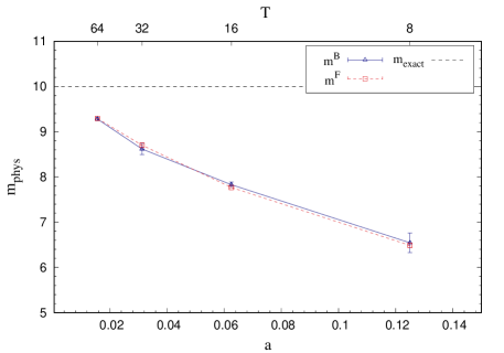
Figure 1: Bosonic and fermionic mass gaps for SUSY harmonic oscillator with physical parameters $m_{\rm phys}=10$ and $g_{\rm phys}=0$ versus lattice spacing ($a$) and lattice size ($T$).

Now we simulate the SUSY anharmonic oscillator for physical parameters $m_{\rm phys}=10$ and $g_{\rm phys}=100$, and $\alpha=0$. Simulations were performed for different lattice spacings keeping the (physical) circle size $\beta=1$. In table 1 we provide the bosonic and fermionic mass gaps. Here also we have $m^{B}_{\text{phys}}\approx m^{F}_{\text{phys}}$ indicating that SUSY is preserved in the model. Table 2 contains the expectation values of the auxiliary field ${\mathcal{B}}_{\alpha}$ and bosonic action $\mathcal{S}^{B}_{\alpha}$. The mean expectation value $\langle{\mathcal{B}}\rangle$ vanishes in the simulations and thus indicate exact lattice SUSY. This table also contains the expectation value of the bosonic action $\mathcal{S}^{B}_{\alpha}$. For this model, we observe $\langle\mathcal{S}^{B}\rangle=\frac{1}{2}T$, and it was independent of physical parameters $g_{\rm phys}$ and $m_{\rm phys}$, which again suggests SUSY is preserved in this model.

Figure 2 shows the bosonic (left) and fermionic (right) correlation functions (used to compute the respective mass gaps) versus lattice site ($t$) for various lattice size ($T$) for the SUSY anharmonic oscillator. In Fig. 3 we show the bosonic and fermionic physical mass gaps versus lattice spacing ($a$) and lattice size ($T$). Here we also compare our results with those obtained by Catterall and Gregory Catterall:2000rv , ($m^{B}_{\rm CG}$, $m^{F}_{\rm CG}$), and find excellent agreement. Black dashed line shows the continuum value of SUSY anharmonic oscillator mass gaps for the physical parameters $m_{\rm phys}=10$, $g_{\rm phys}=100$ that is $m_{\rm exact}$ = 16.865 Bergner:2007pu . We see that boson and fermion masses are degenerate within statistical errors, and furthermore, as lattice spacing $a\to 0$, the common mass gap approaches the correct continuum value. In Fig. 4 we plot the real part of Ward identity $\mathscr{W}_{1}$ (left), and its bosonic and fermionic contributions (right), given in Eq. (3.32), versus the lattice site $t$ for lattices with $T$ values. We observe that the respective bosonic and fermionic contributions cancel each other out within statistical errors, and hence $\mathscr{W}_{1}$ is satisfied. Our results confirm that the SUSY anharmonic oscillator has an exact SUSY, which is responsible for the degenerate mass gaps.

$T$	$a=T^{-1}$	$m^{B}$	$m^{B}_{\text{phys}}=a^{-1}m^{B}$	$m^{F}$	$m^{F}_{\text{phys}}=a^{-1}m^{F}$
8	0.125	$1.0457(65)$	$8.3656(520)$	$1.0247(4)$	$8.1976(32)$
16	0.0625	$0.6852(45)$	$10.9632(720)$	$0.6657(1)$	$10.6512(16)$
32	0.03125	$0.4040(54)$	$12.9280(1664)$	$0.4023(2)$	$12.8736(64)$
64	0.015625	$0.2252(13)$	$14.4128(832)$	$0.2282(3)$	$14.6048(192)$

Table 1: Bosonic and fermionic mass gaps for SUSY anharmonic oscillator. The parameters used are $m_{\rm phys}=10$ and $g_{\rm phys}=100$.

$\Xi^{\prime}(\phi)$	$T$	$a=T^{-1}$	$\alpha$	$~{}\langle{\mathcal{B}}_{\alpha}\rangle$	$~{}\langle\mathcal{S}^{B}_{\alpha}\rangle$
$m\phi+g\phi^{3}$	$8$	$0.1250$	$0.00$	$0.0(0)-i0.0008(38)$	$4.0672(67)+i0.0(0)$
	$16$	$0.0625$	$0.00$	$0.0(0)+i0.0003(68)$	$8.0698(95)+i0.0(0)$
	$32$	$0.03125$	$0.00$	$0.0(0)-i0.0038(131)$	$16.1589(147)+i0.0(0)$
	$64$	$0.015625$	$0.00$	$0.0(0)-i0.0162(245)$	$32.2293(252)+i0.0(0)$

Table 2: Expectation value of the auxiliary field ${\mathcal{B}}_{\alpha}$ and the bosonic action $\mathcal{S}^{B}_{\alpha}$ for SUSY anharmonic oscillator. The parameters used are $m_{\rm phys}=10$ and $g_{\rm phys}=100$.

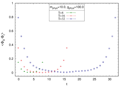
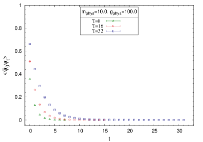
Figure 2: Bosonic (left) and fermionic (right) correlation functions for SUSY anharmonic oscillator. The parameters used are $m_{\rm phys}=10$ and $g_{\rm phys}=100$.

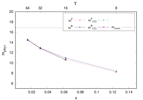
Figure 3: Bosonic and fermionic mass gaps for SUSY anharmonic oscillator. The parameters used are $m_{\rm phys}=10$ and $g_{\rm phys}=100$. Here $m^{B}_{\rm CG}$ and $m^{F}_{\rm CG}$, respectively represent bosonic and fermionic mass-gap results from Ref. Catterall:2000rv .

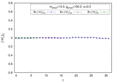
Figure 4: Real part of the Ward identity (left) and real part of the bosonic and fermionic contributions to the Ward identity (right), versus lattice site $t$ for lattices with $T$. Simulations were performed for SUSY anharmonic oscillator with physical parameters $m_{\rm phys}=10$ and $g_{\rm phys}=100$ for lattice sizes $T=8,16$, and $32$.

4.2 General polynomial potential

As a check of our code we consider the model with a degree-$k$ polynomial potential with real coefficients

$${\Xi{{}^{\prime}}}^{(k)}=g_{k}\phi^{k}+g_{k-1}\phi^{k-1}+\cdots+g_{0}.$$ (4.6)

In these systems, it is well known that SUSY is spontaneously broken if the count of zeroes of the potential is even, that is when ${\Xi}^{(k)}(-\infty)$ and ${\Xi}^{(k)}(+\infty)$ have opposite signs Witten:1981nf . For simplicity, we assume the form $g_{k}=g$, $g_{k-1}=\cdots=g_{2}=0$, $g_{1}=m$ and $g_{0}=g\mu^{2}$. Then, for degree $k=4$ and $5$, we have

$${\Xi{{}^{\prime}}}^{(4)} = g\phi^{4}+m\phi+g\mu^{2},$$ (4.7)

$${\Xi{{}^{\prime}}}^{(5)} = g\phi^{5}+m\phi+g\mu^{2}.$$ (4.8)

Using complex CL method, we confirm the analytical prediction that SUSY is broken for even-($k=4$) and preserved for odd-($k=5$) degree real-polynomial potentials.

For even-degree potential we encounter singular drift problem when $\alpha=0$. This shows up in the simulations as the complex Langevin correctness criteria involving the probability of absolute drift not being satisfied. For $\alpha=0$, we obtained a power law decay instead of an exponential decay. Therefore we have performed simulations for various non-zero $\alpha$. Our simulations suggest that above a particular $\alpha$ value the correctness criteria is satisfied and the probability of absolute drift falls off exponentially.

   

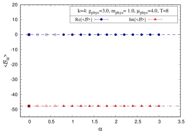
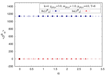
Figure 5: Expectation values of auxiliary field ${\mathcal{B}}_{\alpha}$ (left) and the bosonic action $\mathcal{S}^{B}_{\alpha}$ (right) for various $\alpha$ values on a lattice with $T=8$. The simulations are for the model with even-degree real polynomial potential ${\Xi{{}^{\prime}}}^{(4)}$ given in Eq. (4.7). The parameters used are $g_{\rm phys}=3$, $m_{\rm phys}=1$, and $\mu_{\rm phys}=4$.

In Fig. 5 we show the expectation value of the auxiliary field $\langle{\mathcal{B}}_{\alpha}\rangle$ (left) and the bosonic action $\langle\mathcal{S}^{B}_{\alpha}\rangle$ (right) on a $T=8$ lattice for various $\alpha$ values. We consider the parameter space where CL simulations are justified and take the limit $\alpha\to 0$. The filled data points (red triangles for imaginary part and blue circles for real part) represent expectation values of observables for parameter space where CL can be trusted, while for unfilled data points CL correctness criteria is not satisfied. The lines represent a linear fit of observables for parameter space where CL simulations are justified and solid squares represent values of respective observables in the limit $\alpha\to 0$. These results indicate that $\langle{\mathcal{B}}\rangle$ does not vanish. The expectation value of the bosonic action $\langle\mathcal{S}^{B}\rangle\neq\frac{1}{2}T$, and it is found to be dependent on the physical parameters. These results indicate that SUSY is broken for the even-degree real-polynomial superpotential.

For the model with odd-degree potential, we observe that for $\alpha=0$ the CL correctness criteria are satisfied. In table 3 we provide the simulation results for physical parameter $g_{\rm phys}=3,~{}m_{\rm phys}=1~{}{\rm and}~{}\mu_{\rm phys}=4.0$, on lattices with $T=8,12,16$, and $\alpha=0$. Our simulations gave vanishing value for the auxiliary field expectation value $\langle{\mathcal{B}}\rangle$. We also observed that the expectation value of bosonic action is $\langle\mathcal{S}^{B}\rangle=\frac{1}{2}T$ within errors. It is also independent of the coupling $g$. These results indicate that SUSY is preserved for these models. In Fig. 6 we plot the Ward identities for this model. In these plots, on the left, we show the complete Ward identity (real part), and on the right, we present the respective bosonic and fermionic contributions to the Ward identity. For this model, the bosonic and fermionic contributions cancel each other out within statistical errors, and the Ward identity is thus satisfied. These results indicate unbroken SUSY in this model.

$\Xi^{\prime}(\phi)$	$T$	$a=T^{-1}$	$~{}\langle{\mathcal{B}}_{\alpha}\rangle$	$~{}\langle\mathcal{S}^{B}_{\alpha}\rangle$
	${8}$	${0.25}$	$0.0000(0)+i0.0042(101)$	$4.0214(202)+i0.0000(0)$
${\Xi{{}^{\prime}}}^{(5)}$	${12}$	${0.125}$	$0.0000(0)+i0.0044(74)$	$5.9942(176)+i0.0000(0)$
	${16}$	${0.0833}$	$0.0000(0)-i0.0026(86)$	$8.0398(210)+i0.0000(0)$

Table 3: Expectation value of the auxiliary field ${\mathcal{B}}_{\alpha}$ and the bosonic action $\mathcal{S}^{B}_{\alpha}$ for the odd-degree superpotential ${\Xi{{}^{\prime}}}^{(5)}$. The parameters used are $g_{\rm phys}=3$, $m_{\rm phys}=1$, and $\mu_{\rm phys}=4.0$.

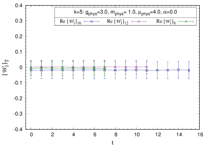
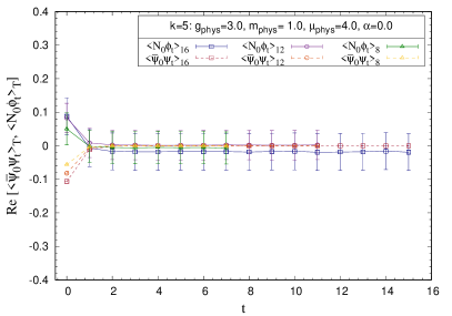
Figure 6: Real part of the Ward identity (left) and real part of bosonic and fermionic contributions to the Ward identity (right) for the model with odd-degree real polynomial potential. The parameters used are $g_{\rm phys}=3$, $m_{\rm phys}=1$, and $\mu_{\rm phys}=4.0$ on lattices with $T=8,12$, and $16$.

4.3 $\mathcal{PT}$-symmetric models

In this section, we simulate an interesting class of complex actions that exhibit, in addition to supersymmetry, $\mathcal{PT}$-symmetry.

Quantum mechanics and quantum field theory are conventionally formulated using Hermitian Hamiltonians and Lagrangians, respectively. In recent years there has been an increasing interest in extensions to non-Hermitian quantum theories Bender:2002vv , particularly those with $\mathcal{PT}$-symmetry Bender:1998ke ; Bender:2005tb , which have real spectra. Such theories have found applications in many areas such as optonics PhysRevLett.105.013903 ; Longhi_2017 and phase transitions Ashida_2017 ; Matsumoto_2020 . Recently, it has been shown that it is possible to carry over the familiar concepts from Hermitian quantum field theory, such as the spontaneous symmetry breaking and the Higgs mechanism in gauge theories, to $\mathcal{PT}$-symmetric non-Hermitian theories PhysRevD.98.045001 ; PhysRevD.99.045006 ; FRING2020114834 . In Ref. Alexandre:2020wki , the authors constructed $\mathcal{PT}$-symmetric ${\cal N}=1$ supersymmetric quantum field theories in $3+1$ dimensions. There, they found that even though the construction of the models are explicitly supersymmetric, they offer a novel non-Hermitian mechanism for soft SUSY breaking.

Imposing $\mathcal{PT}$-symmetric boundary conditions on the functional-integral representation of the four-dimensional $-\lambda\phi^{4}$ theory can give a spectrum that is bounded below Bender:1999ek . Such an interaction leads to a quantum field theory that is perturbatively renormalizable and asymptotically free, with a real and bounded spectrum. These properties suggest that a $-\lambda\phi^{4}$ quantum field theory might be useful in describing the Higgs sector of the Standard Model.

We hope that our investigations would serve as a starting point for exploring the nonperturbative structure of these types of theories in higher dimensions.

The models we consider here have the following potential

$$\Xi(\phi)=-\frac{g}{(2+\delta)}\left(i\phi\right)^{\left(2+\delta\right)},$$ (4.9)

with $\Xi^{{}^{\prime}}(\phi)=-ig~{}(i\phi)^{(1+\delta)}$ and $\delta$ is a continuous parameter. The supersymmetric Lagrangian for this $\mathcal{PT}$-symmetric theory breaks parity symmetry, and it would be interesting to ask whether the breaking of parity symmetry induces a breaking of supersymmetry. This question was answered for the case of a two-dimensional model in Ref. Bender:1997ps . There, through a perturbative expansion in $\delta$, the authors found that supersymmetry remains unbroken in this model. We investigate the absence or presence of non-perturbative SUSY breaking in the one-dimensional cousins of these models using CL method. Clearly, such an investigation based on path integral Monte Carlo fails since the action of this model can be complex, in general.

Even $\delta$ case

We note that when $\delta=0$ the model becomes the supersymmetric harmonic oscillator discussed in Sec. 4.1.

In table 4 we provide the simulation results for $\delta=2,~{}4$. Simulations were performed for physical parameter $g_{\rm phys}=0.5$, on lattices with $T=4,8,12$, and $\alpha=0$. We noticed that the auxiliary field expectation value $\langle{\mathcal{B}}\rangle$ vanishes. We also observe that the expectation value of bosonic action is $\langle\mathcal{S}^{B}\rangle=\frac{1}{2}T$ within errors. It is also independent of the coupling $g$. These results indicate that SUSY is preserved in these models.

$\Xi^{\prime}(\phi)$	$T$	$a=T^{-1}$	$~{}\langle{\mathcal{B}}_{\alpha}\rangle$	$~{}\langle\mathcal{S}^{B}_{\alpha}\rangle$
	${4}$	${0.25}$	$0.0000(0)+i0.0005(282)$	$2.0130(102)+i0.0000(0)$
$\delta=2$	${8}$	${0.125}$	$0.0000(0)+i0.0128(750)$	$4.0326(157)+i0.0000(0)$
	${12}$	${0.0833}$	$0.0000(0)-i0.0071(263)$	$6.0354(58)+i0.0000(0)$
	${4}$	${0.25}$	$0.0000(0)+i0.0167(679)$	$1.9975(47)+i0.0000(0)$
$\delta=4$	${8}$	${0.125}$	$0.0000(0)+i0.0142(567)$	$4.0058(54)+i0.0000(0)$
	${12}$	${0.0833}$	$0.0000(0)-i0.0309(1022)$	$6.0018(74)+i0.0000(0)$

Table 4: Expectation values of the auxiliary field ${\mathcal{B}}_{\alpha}$ and the bosonic action $\mathcal{S}^{B}_{\alpha}$ for the $\mathcal{PT}$-symmetric models with $\delta=2,4$.

In Figs. 7 and 8 we show the Ward identities for $\delta=2,~{}4$, respectively, on a $T=8$ lattice. The full Ward identity $\mathscr{W}_{1}$ is shown on the left panel, and the real and imaginary parts of the bosonic and fermionic contributions to the Ward identity are shown in the middle and right panels. Our simulations show that the bosonic and fermionic contributions cancel each other out within statistical errors, and hence the Ward identities are satisfied. All these results clearly suggest that SUSY is preserved in models with $\mathcal{PT}$-symmetry inspired $\delta$-even potentials.

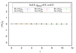
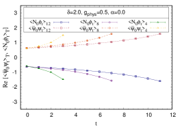
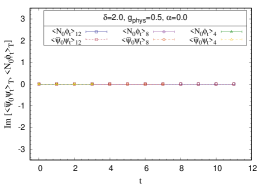
Figure 7: The $\mathcal{PT}$-symmetric model with $\delta=2$. The full Ward identity (left) and real (middle) and imaginary (right) parts of bosonic and fermionic contributions to Ward identity, for lattices with $T=4,8$, and $12$.

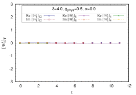
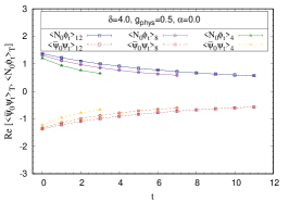
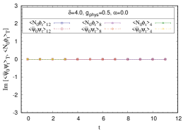
Figure 8: The $\mathcal{PT}$-symmetric model with $\delta=4$. The full Ward identity (left) and real (middle) and imaginary (right) parts of bosonic and fermionic contributions to Ward identity, for lattices with $T=4,8$, and $12$.

Odd $\delta$ case

In these models we had to introduce a deformation parameter to handle the singular drift problem. The results are extracted in the vanishing limit of this parameter.

The simulations were carried out for various non-zero $\mu$, and then the $\delta=1$ model is recovered by taking ${\mu_{\rm phys}\to 0}$ limit. Our simulations suggest that when $\mu_{\rm phys}$ is above a particular value the correctness criteria is satisfied and the probability of absolute drift falls off exponentially. We take in account the $\mu_{\rm phys}$ parameter space where CL simulations are justified and consider the limit $\mu_{\rm phys}\to 0$.

In Fig. 9, we show the expectation values $\langle{\mathcal{B}}\rangle$ (left) and $\langle\mathcal{S}^{B}\rangle$ (right) for a lattice with $T=8$ and for various $\mu_{\rm phys}$ values. The filled data points (red triangles for imaginary part and blue circles for real part) represent expectation values of observables for the parameter space where CL can be trusted, while for unfilled data points where the CL correctness criteria is not satisfied. Lines represent linear fit of observables for parameter space where CL simulations are justified and the solid squares represent values of respective observables in the $\lim\mu_{\rm phys}\to 0$.

These simulation results indicate that $\langle{\mathcal{B}}\rangle$ vanishes in the limit $\mu_{\rm phys}\to 0$. Also, the expectation value of the bosonic action $\langle\mathcal{S}^{B}\rangle=\frac{1}{2}T$ in this limit. It is also found to be independent of the physical parameters. Thus we conclude that SUSY is preserved in the $\delta=1$ model.

   

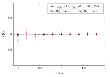
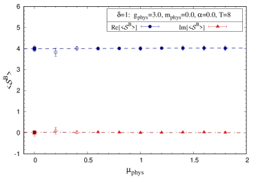
Figure 9: The $\delta=1$ model. Expectation values of ${\mathcal{B}}_{\alpha}$ (left) and $\mathcal{S}^{B}_{\alpha}$ (right) for various $\mu_{\rm phys}$ and $\lim\mu_{\rm phys}\to 0$ on a $T=8$ lattice. Parameters used in the simulations are $g_{\rm phys}=3$, $m_{\rm phys}=0$, and $\alpha=0$.

Now for the $\delta=3$ model, inspired by the idea mentioned in Ref. Ito:2016efb (which was successfully applied in Refs. Anagnostopoulos:2017gos ; Anagnostopoulos:2020xai ) to handle the singular drift problem, we introduce a fermionic deformation term in the action. The fermionic action then becomes

$$\mathcal{S}^{F}=\sum_{i=0}^{T-1}{\overline{\psi}}_{i}\bigg{(}\sum_{j=0}^{T-1}\nabla^{-}_{ij}+d_{f}+\Xi^{{}^{\prime\prime}}_{ij}\bigg{)}\psi_{j},$$ (4.10)

where $d_{f}$ is the deformation parameter.

The values of $d_{f}$ are chosen such that CL correctness criteria are satisfied. The $\delta=3$ model is recovered as ${d_{f}\to 0}$. Our simulations suggest that above a particular $d_{f}$ value the correctness criteria is satisfied and the probability of absolute drift falls off exponentially.

In Fig. 10, we show $\langle{\mathcal{B}}\rangle$ (left) and $\langle\mathcal{S}^{B}\rangle$ (right) on a $T=8$ lattice for various values of $d_{f}$. The filled data points (red triangles for the imaginary part and blue circles for the real part) represent the expectation values of the observables for the parameter space where CL can be trusted, while the corresponding unfilled data points represent the simulation data that do not satisfy the correctness criteria. The dashed curves represent a linear fit for $\langle{\mathcal{B}}\rangle$ data and quadratic fit for $\langle\mathcal{S}^{B}\rangle$ data. The solid squares represent the values of respective observables in the $\lim d_{f}\to 0$ limit. The simulation results suggest that $\langle{\mathcal{B}}\rangle$ vanishes in the $\mu_{\rm phys}\to 0$ limit. Also, $\langle\mathcal{S}^{B}\rangle=\frac{1}{2}T$ within error bars in this limit. It is also found to be independent of the physical parameters of the model. These results indicate that SUSY is preserved in the $\delta=3$ model.

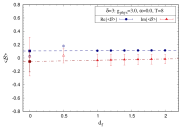
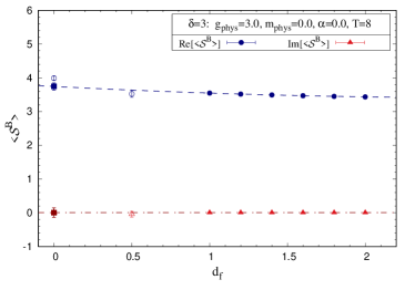
Figure 10: The $\delta=3$ model. Expectation values of ${\mathcal{B}}_{\alpha}$ (left) and $\mathcal{S}^{B}_{\alpha}$ (right) against mass deformation $d_{f}$ parameter on a $T=8$ lattice. The parameters used are $g_{\rm phys}=3$, $m_{\rm phys}=0$, and $\alpha=0.0$. The dashed curves represent extrapolations to the $d_{f}\to 0$ limit.

5 Conclusions

In this paper, using complex Langevin method, we have investigated dynamical SUSY breaking in quantum mechanics models with real and complex actions.

When periodic boundary conditions are used in quantum mechanics with broken SUSY the expectation values of observables are ill-defined. We resolved this problem by using twisted boundary conditions Kuroki:2009yg in our non-perturbative lattice simulations.

We find that for the case of real actions, SUSY is preserved in models with harmonic and anharmonic oscillator potentials, and with odd-powered polynomial potential. SUSY is dynamically broken for the case of even-powered polynomial potential. For the case of supersymmetric anharmonic oscillator, our simulations reproduced the earlier results obtained through Hamiltonian Monte Carlo Catterall:2000rv .

We then moved on to simulate an interesting class of supersymmetric models with complex actions that are ${\cal PT}$-symmetric. Our simulations suggested that SUSY is preserved in these models.

We noticed that during the complex Langevin simulations some of these models suffered from the singular drift problem. In order to overcome this difficulty we introduced appropriate deformation parameters in the models, such that the criteria of correctness of complex Langevin simulations are respected. The target theories are recovered by taking the limits in which the deformation parameters go to zero.

The reliability of the simulations were checked by studying the Langevin operator on observables and the exponential fall off of the drift terms. The results of our investigations on the correctness of the simulations are provided in Appendix A. Our conclusion is that the complex Langevin method can be used reliably to probe non-perturbative SUSY breaking in various quantum mechanics models with real and complex actions.

It would be interesting to extend our investigations to models in higher dimensions, especially quantum field theory systems in four dimensions, such as QCD with finite temperature and baryon/quark chemical potentials. Another long term hope would be to apply these methods to ${\cal PT}$-symmetric supersymmetric quantum field theories in higher dimensions. We hope that these studies may find applications in fundamental physics.

Appendix A Reliability of simulations

In order to monitor the reliability of simulations we use the two recently proposed methods: one tracks the vanishing nature of the Fokker-Planck operator Aarts:2009uq ; Aarts:2011ax ; Aarts:2013uza and the other monitors the decay of the probability distribution of the drift term magnitude Nagata:2016vkn ; Nagata:2018net .

A.1 Langevin operator on observables

The observables of the theory ${\cal O}_{i}[\phi,\theta]$ at $i$-th site evolve in the following way

$$\frac{\partial{\cal O}_{i}[\phi,\theta]}{\partial\theta}=\widetilde{L}_{i}{\cal O}_{i}[\phi,\theta],$$ (A.1)

where $\widetilde{L}_{i}$ is the Langevin operator for the $i$-th site. It is defined as

$$\widetilde{L}_{i}=\left(\frac{\partial}{\partial\phi_{i}}-\frac{\partial\mathcal{S}^{\rm eff}[\phi]}{\partial\phi_{i}}\right)\ \frac{\partial}{\partial\phi_{i}}.$$ (A.2)

Once the equilibrium distribution is reached, we can remove the $\theta$ dependence from the observables. Then we have $C_{{\cal O}_{i}}\equiv\langle\widetilde{L}_{i}{\cal O}_{i}[\phi]\rangle=0$, and this can be used as a criterion for correctness of the simulations. This criterion was used to study various interesting models in Refs. Aarts:2009uq ; Aarts:2011ax ; Aarts:2013uza .

If we take ${\mathcal{B}}_{i}$ at the $i$-th site as the observable then we have

$$\widetilde{L}_{i}{\mathcal{B}}_{i}=-i\Xi^{{}^{\prime\prime\prime}}_{iii}+i\Xi^{{}^{\prime\prime}}_{ii}\frac{\partial\mathcal{S}^{\rm eff}}{\partial\phi_{i}}.$$ (A.3)

Note that $\widetilde{L}{\mathcal{B}}$ respects translational symmetry on the lattice, and hence we can monitor the value obtained by averaging over all lattice sites.

In table 5 we provide the expectation values of $\widetilde{L}{\mathcal{B}}$ for the simulations of supersymmetric anharmonic oscillator model discussed in Sec. 4.1. We see that this observable is zero within error bars and thus we can trust the simulations.

$\Xi^{\prime}(\phi)$	$T$	$a=T^{-1}$	$~{}\langle\widetilde{L}{\mathcal{B}}_{\alpha}\rangle$
$m\phi+g\phi^{3}$	8	0.125	$0.0000(0)+i0.0268(910)$
	16	0.0625	$0.0000(0)-i0.0379(450)$
	32	0.03125	$0.0000(0)+i0.0131(232)$
	64	0.015625	$0.0000(0)+i0.0056(132)$

Table 5: Expectation value of $\widetilde{L}{\mathcal{B}}_{\alpha}$ for supersymmetric anharmonic oscillator with parameters $m_{\rm phys}=10.0$ and $g_{\rm phys}=100.0$. Simulations were performed for different lattice spacings with $\beta=1$ and $\alpha=0$.

In Fig. 11, we show the expectation values $\widetilde{L}{\mathcal{B}}$ for various twist parameter values for the model with case of real even-degree ($k=4$) polynomial potential (discussed in Sec. 4.2). The filled data points (red triangles for imaginary part and blue circles for real part) represent expectation values of $\widetilde{L}{\mathcal{B}}$ for the parameter space where CL can be trusted, when the second criterion, decay-of-the-drift-term, to be discussed in the next section, is applied. The unfilled data points represent the expectation values of $\widetilde{L}{\mathcal{B}}$ in the parameter space where the decay-of-the-drift-term criterion is not satisfied.

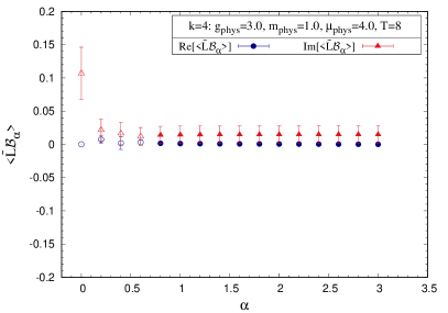
Figure 11: Expectation values of $\widetilde{L}{\mathcal{B}}_{\alpha}$ for various $\alpha$ values, on a $T=8$ lattice, for the model with even-degree ($k=4$) polynomial potential, given in Eq. (4.7). The parameters used are $g_{\rm phys}=3$, $m_{\rm phys}=1$, and $\mu_{\rm phys}=4.0$.

In table 6 we provide the expectation values of $\widetilde{L}{\mathcal{B}}$ for the simulations of real odd-degree ($k=5$) polynomial potentials discussed in Sec. 4.2. We see that this observable is zero within error bars and thus we can trust the simulations.

$\Xi^{\prime}(\phi)$	$T$	$a=T^{-1}$	$~{}\langle\widetilde{L}{\mathcal{B}}_{\alpha}\rangle$
	8	0.125	$0.0000(0)-i0.0010(729)$
${\Xi{{}^{\prime}}}^{(5)}$	12	0.0833	$0.0000(0)+i0.0127(508)$
	16	0.0625	$0.0000(0)-i0.0301(396)$

Table 6: Expectation values of $\widetilde{L}{\mathcal{B}}_{\alpha}$ for the model with odd-degree ($k=5$) real-polynomial potential given in Eq. (4.8). The parameters used are $g_{\rm phys}=3$, $m_{\rm phys}=1$, and $\mu_{\rm phys}=4.0$.

In table 7 we show the expectation values of $\widetilde{L}{\mathcal{B}}$ for $\mathcal{PT}$ symmetric models with $\delta=2$ and 4.

$\Xi^{\prime}(\phi)$	$T$	$a=T^{-1}$	$\langle\widetilde{L}{\mathcal{B}}_{\alpha}\rangle$
	${4}$	${0.25}$	$-0.0000(0)-i0.0104(72)$
$\delta={2}$	${8}$	${0.125}$	$-0.0000(0)+i0.0006(59)$
	${12}$	${0.0833}$	$-0.0000(0)-i0.0104(72)$
	${4}$	${0.25}$	$0.0000(0)+i0.0403(244)$
$\delta={4}$	${8}$	${0.125}$	$0.0000(0)+i0.0027(91)$
	${12}$	${0.0833}$	$0.0000(0)-i0.0098(64)$

Table 7: Expectation value of $\widetilde{L}{\mathcal{B}}_{\alpha}$ for the $\mathcal{PT}$-symmetric potentials given in Eq. (4.9) with $\delta=2$ and 4. The simulation parameters used are $\beta=1$, $g_{\rm phys}=0.5$, and $\alpha=0$.

In Fig. 12 (left), we show the expectation values for various $\mu_{\rm phys}$ values of $\widetilde{L}{\mathcal{B}}$ for the simulations of $\delta=1$ model. The filled (unfilled) data points represent the simulations that does (does not) respect the decay-of-the-drift-term criterion. In Fig. 12, (right) we show $\widetilde{L}{\mathcal{B}}$ for various deformation parameter $d_{f}$ for the $\delta=3$ model. Again, the filled (unfilled) data points represent the simulations that does (does not) respect the decay-of-the-drift-term criterion.

 

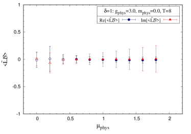
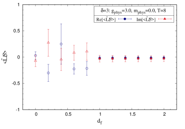
Figure 12: Expectation values of $\widetilde{L}{\mathcal{B}}_{\alpha}$ for the $\mathcal{PT}$ symmetric model on a $T=8$ lattice. (Left) Case $\delta=1$. (Right) Case $\delta=3$. The parameters used are $g_{\rm phys}=3$, $m_{\rm phys}=0$, and $\alpha=0.0$.

A.2 Decay of the drift terms

The decay-of-the-drift-term criterion was proposed in Refs. Nagata:2016vkn ; Nagata:2018net . There, the authors demonstrated, in a few simple models, that the probability of the drift term should be suppressed exponentially or faster at larger magnitudes to guarantee the correctness of the CL method.

The magnitude of the mean drift is defined as

$$u\equiv\sqrt{\frac{1}{T}\sum_{i=0}^{T-1}\left|\frac{\partial\mathcal{S}^{\text{eff}}}{\partial\phi_{i}}\right|^{2}}.$$ (A.4)

In our work, to avoid the singular drift problem, we introduced appropriate deformation parameters in the theory. The final results are obtained after extrapolating to the vanishing limits of deformation parameters.

In Fig. 13, we show the probability distribution $P(u)$ against $u$ for the simulations of supersymmetric anharmonic (left) and harmonic (right) potentials discussed in Sec. 4.1. We see that the drift terms decay exponentially or faster in these models and thus the simulations can be trusted.

 

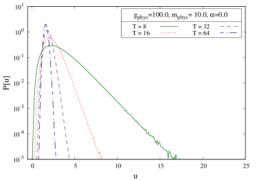
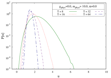
Figure 13: The decay of the drift terms. (Left) Supersymmetric anharmonic oscillator with the parameters $m_{\rm phys}=10.0$ and $g_{\rm phys}=100.0$. (Right) supersymmetric harmonic oscillator with parameters $m_{\rm phys}=10.0$ and $g_{\rm phys}=0.0$.

In Fig. 14 (left) we show the decay of drift terms for various $\alpha$ values, for the model with even-degree ($k=4$) real polynomial potential. We see that the drift terms decay exponentially or faster when $\alpha\geq 0.8$ and the simulations can be trusted in this parameter regime. In Fig. 14 (right) we show the decay of drift terms for various $\alpha$ values, for the model with even-degree ($k=5$) real polynomial potential. We see that the drift terms decay exponentially or faster when $\alpha=0$ and the simulations can be trusted in this parameter regime.

 

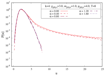
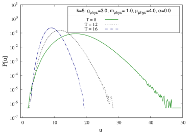
Figure 14: (Left) Decay of the drift term for various $\alpha$ values for the model with even-degree ($k=4$) polynomial potential on a $T=8$ lattice. The parameters used are $g_{\rm phys}=3$, $m_{\rm phys}=1$, and $\mu_{\rm phys}=4.0$. (Right) The decay of the drift terms for the model with odd-degree ($k=5$) real polynomial potential on $T=8,12,16$ lattices. The parameters used are $g_{\rm phys}=3$, $m_{\rm phys}=1$, and $\mu_{\rm phys}=4.0$.

In Fig. 15 we show The drift term decay for the $\mathcal{PT}$ symmetric models with $\delta=2$ (left) and $\delta=4$ (right). The drift terms decay exponentially or faster when $\alpha=0$. Thus the simulations can be trusted in this parameter regime.

 

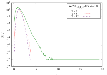
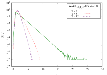
Figure 15: Decay of the drift terms for the $\mathcal{PT}$ symmetric models with $\delta=2$ (left) and $\delta=4$ (right). The parameters used are $g_{\rm phys}=0.5$ and $\alpha=0$.

In Fig. 16 (left) we show the drift term decay for the $\mathcal{PT}$ symmetric model with $\delta=1$, for various $\mu_{\rm phys}$ values. The drift terms decay exponentially or faster when $\mu_{\rm phys}\geq 0.6$. Thus the simulations can be trusted in this parameter regime. In Fig. 16 (right) we show the decay of the drift terms for various values of the fermionic mass deformation parameter $d_{f}$, for the $\mathcal{PT}$ symmetric model with $\delta=3$. Here we see that the drift terms decay exponentially or faster when $d_{f}>1.0$ and thus the simulations can be trusted in this parameter regime.

 

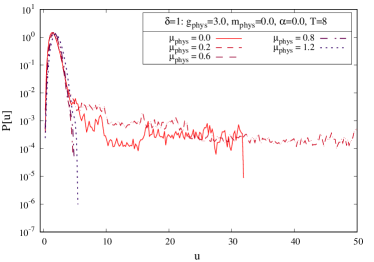
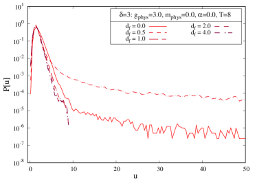
Figure 16: The decay of the drift terms for the $\mathcal{PT}$ symmetric models with odd $\delta$ on $T=8$ lattice. The parameters used were $g_{\rm phys}=3$, $m_{\rm phys}=0$, and $\alpha=0.0$. (Left) The $\delta=1$ case. Simulations were performed for various $\mu_{\rm phys}$ values. (Right) The $\delta=3$ case. Simulations were performed for various values of the fermionic mass deformation parameter $d_{f}$.

References

- (1) E. Witten, Dynamical Breaking of Supersymmetry, Nucl. Phys. B188 (1981) 513.
- (2) E. Witten, Constraints on Supersymmetry Breaking, Nucl. Phys. B 202 (1982) 253.
- (3) P. de Forcrand and O. Philipsen, The QCD phase diagram for small densities from imaginary chemical potential, Nucl. Phys. B 642 (2002) 290 [hep-lat/0205016].
- (4) M. Cristoforetti, F. Di Renzo and L. Scorzato, New approach to the sign problem in quantum field theories: High density qcd on a lefschetz thimble, Phys. Rev. D 86 (2012) 074506.
- (5) J.R. Klauder, Stochastic Quantization, Acta Phys. Austriaca Suppl. 25 (1983) 251.
- (6) J.R. Klauder, A Langevin Approach to Fermion and Quantum Spin Correlation Functions, J. Phys. A16 (1983) L317.
- (7) J.R. Klauder, Coherent State Langevin Equations for Canonical Quantum Systems With Applications to the Quantized Hall Effect, Phys. Rev. A29 (1984) 2036.
- (8) G. Parisi, On complex probabilities, Phys. Lett. 131B (1983) 393.
- (9) P.H. Damgaard and H. Huffel, Stochastic Quantization, Phys. Rept. 152 (1987) 227.
- (10) AuroraScience collaboration, New approach to the sign problem in quantum field theories: High density QCD on a Lefschetz thimble, Phys. Rev. D86 (2012) 074506 [1205.3996].
- (11) H. Fujii, D. Honda, M. Kato, Y. Kikukawa, S. Komatsu and T. Sano, Hybrid Monte Carlo on Lefschetz thimbles - A study of the residual sign problem, JHEP 10 (2013) 147 [1309.4371].
- (12) F. Di Renzo and G. Eruzzi, Thimble regularization at work: from toy models to chiral random matrix theories, Phys. Rev. D92 (2015) 085030 [1507.03858].
- (13) Y. Tanizaki, Y. Hidaka and T. Hayata, Lefschetz-thimble analysis of the sign problem in one-site fermion model, New J. Phys. 18 (2016) 033002 [1509.07146].
- (14) H. Fujii, S. Kamata and Y. Kikukawa, Monte Carlo study of Lefschetz thimble structure in one-dimensional Thirring model at finite density, JHEP 12 (2015) 125 [1509.09141].
- (15) A. Alexandru, G. Basar and P. Bedaque, Monte Carlo algorithm for simulating fermions on Lefschetz thimbles, Phys. Rev. D93 (2016) 014504 [1510.03258].
- (16) J.R. Klauder and W.P. Petersen, Numerical Integration of Multiplicative-Noise Stochastic Differential Equations, SIAM J. Num. Anal. 22 (1985) 1153.
- (17) J.R. Klauder and W.P. Petersen, Spectrum of certain non-self-adjoint operators and solutions of Langevin equations with complex drift, J. Stat. Phys. 39 (1985) 53.
- (18) H. Gausterer and J.R. Klauder, Complex Langevin Equations and Their Applications to Quantum Statistical and Lattice Field Models, Phys. Rev. D33 (1986) 3678.
- (19) G. Aarts, F.A. James, E. Seiler and I.-O. Stamatescu, Complex Langevin: Etiology and Diagnostics of its Main Problem, Eur. Phys. J. C71 (2011) 1756 [1101.3270].
- (20) G. Aarts, E. Seiler and I.-O. Stamatescu, The Complex Langevin method: When can it be trusted?, Phys. Rev. D81 (2010) 054508 [0912.3360].
- (21) K. Nagata, J. Nishimura and S. Shimasaki, Justification of the complex Langevin method with the gauge cooling procedure, PTEP 2016 (2016) 013B01 [1508.02377].
- (22) G. Aarts, F.A. James, E. Seiler and I.-O. Stamatescu, Adaptive stepsize and instabilities in complex Langevin dynamics, Phys. Lett. B 687 (2010) 154 [0912.0617].
- (23) C.E. Berger, L. RammelmŸller, A.C. Loheac, F. Ehmann, J. Braun and J.E. Drut, Complex Langevin and other approaches to the sign problem in quantum many-body physics, 1907.10183.
- (24) J. Berges and I.O. Stamatescu, Simulating nonequilibrium quantum fields with stochastic quantization techniques, Phys. Rev. Lett. 95 (2005) 202003 [hep-lat/0508030].
- (25) J. Berges, S. Borsanyi, D. Sexty and I.O. Stamatescu, Lattice simulations of real-time quantum fields, Phys. Rev. D75 (2007) 045007 [hep-lat/0609058].
- (26) J. Berges and D. Sexty, Real-time gauge theory simulations from stochastic quantization with optimized updating, Nucl. Phys. B799 (2008) 306 [0708.0779].
- (27) J. Bloch, J. Glesaaen, J.J.M. Verbaarschot and S. Zafeiropoulos, Complex Langevin Simulation of a Random Matrix Model at Nonzero Chemical Potential, JHEP 03 (2018) 015 [1712.07514].
- (28) G. Aarts and I.-O. Stamatescu, Stochastic quantization at finite chemical potential, JHEP 09 (2008) 018 [0807.1597].
- (29) C. Pehlevan and G. Guralnik, Complex Langevin Equations and Schwinger-Dyson Equations, Nucl. Phys. B 811 (2009) 519 [0710.3756].
- (30) G. Aarts, Can stochastic quantization evade the sign problem? The relativistic Bose gas at finite chemical potential, Phys. Rev. Lett. 102 (2009) 131601 [0810.2089].
- (31) G. Aarts, Complex Langevin dynamics at finite chemical potential: Mean field analysis in the relativistic Bose gas, JHEP 05 (2009) 052 [0902.4686].
- (32) G. Aarts and K. Splittorff, Degenerate distributions in complex Langevin dynamics: one-dimensional QCD at finite chemical potential, JHEP 08 (2010) 017 [1006.0332].
- (33) G. Aarts and F.A. James, Complex Langevin dynamics in the SU(3) spin model at nonzero chemical potential revisited, JHEP 01 (2012) 118 [1112.4655].
- (34) Y. Ito and J. Nishimura, The complex Langevin analysis of spontaneous symmetry breaking induced by complex fermion determinant, JHEP 12 (2016) 009 [1609.04501].
- (35) Y. Ito and J. Nishimura, Spontaneous symmetry breaking induced by complex fermion determinant — yet another success of the complex Langevin method, PoS LATTICE2016 (2016) 065 [1612.00598].
- (36) K.N. Anagnostopoulos, T. Azuma, Y. Ito, J. Nishimura and S.K. Papadoudis, Complex Langevin analysis of the spontaneous symmetry breaking in dimensionally reduced super Yang-Mills models, JHEP 02 (2018) 151 [1712.07562].
- (37) K.N. Anagnostopoulos, T. Azuma, Y. Ito, J. Nishimura, T. Okubo and S. Kovalkov Papadoudis, Complex Langevin analysis of the spontaneous breaking of 10D rotational symmetry in the Euclidean IKKT matrix model, JHEP 06 (2020) 069 [2002.07410].
- (38) P. Basu, K. Jaswin and A. Joseph, Complex Langevin Dynamics in Large Unitary Matrix Models, Phys. Rev. D98 (2018) 034501 [1802.10381].
- (39) D.J. Gross and E. Witten, Possible Third Order Phase Transition in the Large N Lattice Gauge Theory, Phys. Rev. D21 (1980) 446.
- (40) S.R. Wadia, A Study of U(N) Lattice Gauge Theory in 2-dimensions, 1212.2906.
- (41) S.R. Wadia, = Infinity Phase Transition in a Class of Exactly Soluble Model Lattice Gauge Theories, Phys. Lett. 93B (1980) 403.
- (42) A. Joseph and A. Kumar, Complex Langevin Simulations of Zero-dimensional Supersymmetric Quantum Field Theories, Phys. Rev. D 100 (2019) 074507 [1908.04153].
- (43) T. Kuroki and F. Sugino, Spontaneous supersymmetry breaking in large-N matrix models with slowly varying potential, Nucl. Phys. B 830 (2010) 434 [0909.3952].
- (44) D. Baumgartner and U. Wenger, Supersymmetric quantum mechanics on the lattice: I. Loop formulation, Nucl. Phys. B 894 (2015) 223 [1412.5393].
- (45) G. Bergner, T. Kaestner, S. Uhlmann and A. Wipf, Low-dimensional Supersymmetric Lattice Models, Annals Phys. 323 (2008) 946 [0705.2212].
- (46) S. Catterall and E. Gregory, A Lattice path integral for supersymmetric quantum mechanics, Phys. Lett. B 487 (2000) 349 [hep-lat/0006013].
- (47) I. Kanamori, F. Sugino and H. Suzuki, Observing dynamical supersymmetry breaking with euclidean lattice simulations, Prog. Theor. Phys. 119 (2008) 797 [0711.2132].
- (48) S. Catterall, Lattice supersymmetry and topological field theory, JHEP 05 (2003) 038 [hep-lat/0301028].
- (49) J. Giedt, R. Koniuk, E. Poppitz and T. Yavin, Less naive about supersymmetric lattice quantum mechanics, JHEP 12 (2004) 033 [hep-lat/0410041].
- (50) T. Kuroki and F. Sugino, Spontaneous supersymmetry breaking in matrix models from the viewpoints of localization and Nicolai mapping, Nucl. Phys. B 844 (2011) 409 [1009.6097].
- (51) J. Nishimura and S. Shimasaki, New Insights into the Problem with a Singular Drift Term in the Complex Langevin Method, Phys. Rev. D 92 (2015) 011501 [1504.08359].
- (52) S. Catterall and S. Karamov, Exact lattice supersymmetry: The Two-dimensional N=2 Wess-Zumino model, Phys. Rev. D 65 (2002) 094501 [hep-lat/0108024].
- (53) S. Catterall, D.B. Kaplan and M. Unsal, Exact lattice supersymmetry, Phys. Rept. 484 (2009) 71 [0903.4881].
- (54) D. Kadoh and K. Nakayama, Direct computational approach to lattice supersymmetric quantum mechanics, Nucl. Phys. B 932 (2018) 278 [1803.07960].
- (55) M. Hanada, J. Nishimura and S. Takeuchi, Non-lattice simulation for supersymmetric gauge theories in one dimension, Phys. Rev. Lett. 99 (2007) 161602 [0706.1647].
- (56) C.M. Bender, D.C. Brody and H.F. Jones, Complex extension of quantum mechanics, Phys. Rev. Lett. 89 (2002) 270401 [quant-ph/0208076].
- (57) C.M. Bender and S. Boettcher, Real spectra in non-Hermitian Hamiltonians having PT symmetry, Phys. Rev. Lett. 80 (1998) 5243 [physics/9712001].
- (58) C.M. Bender, Introduction to PT-Symmetric Quantum Theory, Contemp. Phys. 46 (2005) 277 [quant-ph/0501052].
- (59) S. Longhi, Optical Realization of Relativistic Non-Hermitian Quantum Mechanics, Phys. Rev. Lett. 105 (2010) 013903.
- (60) S. Longhi, Parity-time symmetry meets photonics: A new twist in non-Hermitian optics, EPL (Europhysics Letters) 120 (2017) 64001.
- (61) Y. Ashida, S. Furukawa and M. Ueda, Parity-time-symmetric quantum critical phenomena, Nature Communications 8 (2017) .
- (62) N. Matsumoto, K. Kawabata, Y. Ashida, S. Furukawa and M. Ueda, Continuous Phase Transition without Gap Closing in Non-Hermitian Quantum Many-Body Systems, Physical Review Letters 125 (2020) .
- (63) J. Alexandre, J. Ellis, P. Millington and D. Seynaeve, Spontaneous symmetry breaking and the Goldstone theorem in non-Hermitian field theories, Phys. Rev. D 98 (2018) 045001.
- (64) P.D. Mannheim, Goldstone bosons and the Englert-Brout-Higgs mechanism in non-Hermitian theories, Phys. Rev. D 99 (2019) 045006.
- (65) A. Fring and T. Taira, Goldstone bosons in different PT-regimes of non-Hermitian scalar quantum field theories, Nuclear Physics B 950 (2020) 114834.
- (66) J. Alexandre, J. Ellis and P. Millington, -symmetric non-Hermitian quantum field theories with supersymmetry, Phys. Rev. D 101 (2020) 085015 [2001.11996].
- (67) C.M. Bender, K.A. Milton and V.M. Savage, Solution of Schwinger-Dyson equations for PT symmetric quantum field theory, Phys. Rev. D 62 (2000) 085001 [hep-th/9907045].
- (68) C.M. Bender and K.A. Milton, Model of supersymmetric quantum field theory with broken parity symmetry, Phys. Rev. D57 (1998) 3595 [hep-th/9710076].
- (69) N.S. Dhindsa and A. Joseph, Probing Non-perturbative Supersymmetry Breaking through Lattice Path Integrals, 2011.08109.
- (70) D. Kadoh and N. Ukita, General solution of the cyclic Leibniz rule, PTEP 2015 (2015) 103B04 [1503.06922].
- (71) D. Kadoh and K. Nakayama, Lattice study of supersymmetry breaking in supersymmetric quantum mechanics, Nucl. Phys. B 949 (2019) 114783 [1812.10642].
- (72) D. Kadoh, T. Kamei and H. So, Numerical analyses of supersymmetric quantum mechanics with a cyclic Leibniz rule on a lattice, PTEP 2019 (2019) 063B03 [1904.09275].
- (73) G. Aarts, P. Giudice and E. Seiler, Localised distributions and criteria for correctness in complex Langevin dynamics, Annals Phys. 337 (2013) 238 [1306.3075].
- (74) K. Nagata, J. Nishimura and S. Shimasaki, Argument for justification of the complex Langevin method and the condition for correct convergence, Phys. Rev. D94 (2016) 114515 [1606.07627].
- (75) K. Nagata, J. Nishimura and S. Shimasaki, Testing the criterion for correct convergence in the complex Langevin method, JHEP 05 (2018) 004 [1802.01876].