Combining GANs and AutoEncoders
for Efficient Anomaly Detection

Abstract

In this work, we propose CBiGAN — a novel method for anomaly detection in images, where a consistency constraint is introduced as a regularization term in both the encoder and decoder of a BiGAN. Our model exhibits fairly good modeling power and reconstruction consistency capability. We evaluate the proposed method on MVTec AD — a real-world benchmark for unsupervised anomaly detection on high-resolution images — and compare against standard baselines and state-of-the-art approaches. Experiments show that the proposed method improves the performance of BiGAN formulations by a large margin and performs comparably to expensive state-of-the-art iterative methods while reducing the computational cost. We also observe that our model is particularly effective in texture-type anomaly detection, as it sets a new state of the art in this category. Our code is available at https://github.com/fabiocarrara/cbigan-ad/.

I Introduction

In the era of large-scale datasets, the ability to automatically detect outliers (or anomalies) in data is relevant in many application fields. Recognizing anomalous textures is often required e.g. for the detection of defects in industrial manufacturing [1, 2] and large-scale infrastructural maintenance of roads, bridges, rails, etc, while other applications require the detection of more complex shapes and structures, like biomedical applications [3, 4] dealing for example with early disease detection via medical imaging. Even if this problem could be tackled with discriminative approaches — e.g. as a supervised binary classification problem in which samples can be classified as normal or anomalous — the cost of collecting a representative training dataset, especially anomalous samples, is often prohibitive. Thus, interest has grown for one-class anomaly detection. This is often cast as a learning problem where normal data is modelled exploiting generative approaches, relying on an unlabeled dataset mostly comprised of non-anomalous samples.

Recent developments in deep learning and image representation has introduced visual anomaly detection in many applications as for instance biomedical (e.g. diagnoses aids) and industrial (e.g. quality assurance) applications. In these applications, classical approaches to anomaly detection, such as statistical-based [5, 6], proximity-based [7, 8], or clustering-based [9, 10] approaches, often offer poor performance when applied directly to images, due to the high-dimensionality involved in this type of data, and usually have to rely on the extraction of lower-dimensional hand-crafted or learned features.

Recent approaches directly adopt deep models to contextually map and model the data in a feature space. In this context, deep generative models for images based on Autoencoders (AEs) [11, 12] or Generative Adversarial Networks (GANs) [4, 13, 14] proved to be effective in anomaly detection. Most approaches in this category are reconstruction-based: starting from a given sample, they reconstruct the nearest sample on the normal data manifold learned by the model and measure the deviation in a predefined space (e.g. pixel, latent, or combinations) to assess an anomaly. Autoencoder-based approaches implement this strategy in a straightforward way: the encoder projects the given sample in the normal data manifold, while the decoder performs the reconstruction. However, generative models based on autoencoders like VAEs are known to produce blurry reconstructions for photo-realistic images [15] and are often outperformed by GANs; thus in this work, we focus our attention on GAN-based approaches for one-class anomaly detection.

	Query	Reconstruction	Abs. Difference
Texture - Grid
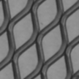
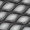
Object - Screw

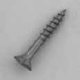
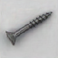
Figure 1: Misaligned reconstructions of a standard BiGAN anomaly detector (EGBAD [16]) that induce a large distance in pixel space. The consistency loss introduced in CBiGAN solves this problem.

Input reconstruction in GAN-based approaches poses a challenge as, in the standard formulation, there is no encoder that projects the sample in the latent space, and an expensive latent space optimization is often required [4]. Efficient approaches based on Bidirectional GANs (BiGAN) solve this problem by jointly learning an encoder that complements the decoder (i.e. generator) and provide the projection needed (e.g. EGBAD [16]). However, reconstructed samples are often misaligned: the reconstruction goal is only defined by the discriminator, and there is no guarantee that encoding and then decoding a sample will reconstruct it precisely (see Figure 1).

In this work, we tackle the aforementioned problems and propose a novel method for anomaly detection in images, where we introduce a consistency constraint as a regularization term, on both encoding and decoding parts of a BiGAN. In the reminder of the paper we call our model CBiGAN. Our new formulation is able to improve the reconstruction ability with respect to a BiGAN. It also generalizes both EGBAD [16] and AEs by combining the modelling power of the former and the reconstruction consistency of the latter. We evaluate the proposed method on MVTec AD — a real-world benchmark for unsupervised anomaly detection on high-resolution images — and compare against standard baselines and state-of-the-art approaches. Our results show that the proposed method solves misalignment problems commonly occurring in GAN formulations improving the performance of BiGAN for complex objects by a large margin. Moreover, our proposal performs comparably to expensive state-of-the-art iterative methods while reducing computational cost requiring a single-pass evaluation strategy. We observe that our model is particularly effective on texture-type anomaly detection, as it sets a new state of the art in this category outperforming also models using additional data.

II Related Work

Most of recent approaches for anomaly detection on images adopt reconstruction-based techniques relying on some sort of deep generative models. Autoencoders (standard [17, 18, 11] and variational ones [19, 12]) and generative adversarial networks [4, 14, 16] comprise the most commonly adopted techniques: the former are trained to minimize a reconstruction loss usually in the pixel space, while the latter focus on generating samples indistinguishable from normal data indirectly leading to reconstruction. Anomaly detection is then implemented by defining a score based on reconstruction error and additional metrics, such as feature matching in latent or intermediate space. Concerning AE techniques, Bergmann et al. [11] point out that dependencies between pixels are not properly modelled in autoencoders and show that vanilla AEs using a structural similarity index metric (SSIM) loss outperform even complex architectures (e.g. AEs with feature matching and VAEs) that rely on L2 pixel-wise losses. In [20], the authors instead proposed bayesian convolutional autoencoders: they show that sampling in variational models smooths noisy reconstruction error compared to other AE architectures on medical data. Zimmerer et al. [21] suggest that the gradient w.r.t the input image of the KL-loss in VAE provides useful information on the normality of data and adopt it for anomaly localization. Building on this concept, Dehaene et al. [19] propose to iteratively integrate these gradients to perform reconstruction by moving samples towards the normality manifold in pixel-space in a similar manner used by adversarial example crafting. Golan and El-Yaniv [22] set up a self-supervised multi-classification pretext task of geometric transformation recognition and use the softmax output on transformed samples as feature to characterize abnormality. Similarly, Huang et al. [23] propose to train a deep architecture to invert geometric transformation of the input and uses the reconstruction error as anomaly score for the input image.

In our work, we build upon GAN-based anomaly detection — techniques that exploit GANs to learn the anomaly-free distribution of data assuming a uniformly or normally distributed latent space explaining it. We focus on the scenario in which we assume a mostly anomaly-free training dataset, and we refer the interested reader to Berg et al. [24] for an analysis of GAN-based detectors when this assumption does not hold. Among the seminal works in this category, Schlegl et al. [4] proposed AnoGAN: the generator is used to perform reconstruction, and the discriminator to extract features of original and reconstructed samples; both are then adopted to define an anomaly score. The major drawback of this approach is the need of a computational expensive latent space optimization using backpropagation to find the latent space representation that encodes the given sample. Recent work solve this problem by introducing an encoding module that learns to map samples from the input to the latent space. Schlegl et al. [13] propose fast-AnoGAN — an enhanced AnoGAN with a learned encoding module and adopting the more stable Wasserstein GAN formulation. Akcay et al. [14] propose an adversarially trained encoder-decoder-encoder architecture named GANomaly and define their anomaly score as the L1 error in the latent space between original and reconstructed sample. Zenati et al. [16] propose EGBAD (Efficient GAN Based Anomaly Detection) that directly adopts a Bidirectional GAN (BiGANs [25]) — an improved GAN formulation that learns the joint distribution of the latent and input spaces — and adopt a combination of reconstruction loss and discriminator loss as anomaly score. In a similar vein, several works propose different architectures that implement some sort of adversarial training [26, 27, 12, 28]. Sabokrou et al. [26] propose a self-supervised approach for anomaly localization that adopts adversarially-trained fully convolutional network plus a discriminator to detect anomalous pixels. Venkataramanan et al. [27] propose an adversarially-trained variational autoencoder combined with a specialized attention regularization that encourages the network to model all the parts of the normal input and thus perform precise anomaly localization.

III Background

III-A Generative Adversarial Networks

In its basic formulation, a Generative Adversarial Network (GAN [29]) is comprised of a generator $G(\mathbf{z})$ that generates data starting from a latent variable $\mathbf{z}\sim p(\mathbf{z})$ and a discriminator $D(\mathbf{x})$ that discerns whether its input $\mathbf{x}$ is generated by $G$ or coming from the real data distribution $p_{\text{data}}(\mathbf{x})$. $G$ and $D$ are adversarially trained to compete — $G$ is optimized to fool $D$, while $D$ to tell apart data generated by $G$ and real one. In a game-theoretic framework, $G$ and $D$ plays the following two-player minimax game

$$\min_{G}\max_{D}\mathbb{E}_{\mathbf{x}\sim p_{\text{data}}(\mathbf{x})}\left[{\log D(\mathbf{x})}\right]+\mathbb{E}_{\mathbf{z}\sim p(\mathbf{z})}\left[{\log\left(1-D\left(G(\mathbf{z})\right)\right)}\right]\,,$$ (1)

where $D(\mathbf{x})\in[0,1]$ indicates how real the discriminator this its input is. At the Nash equilibrium of the game, $D$ is not able to discern fake samples from real ones, and thus, $G$ is producing samples from $p_{\text{data}}(\mathbf{x})$.

III-B Wasserstein GAN

Reaching the Nash equilibrium is known to be hard due to training instabilities [30]. Wasserstein GAN (WGAN [31]) facilitates GAN training by measuring the distance between real and fake data distributions using the Wasserstein distance that assures more stable gradients. In this formulation, $D(\mathbf{x})\in\mathbb{R}$ is defined as a scalar helper function used to compute the Wasserstein distance that substitutes the value function in the minimax game

$$\min_{G}\max_{D}\mathbb{E}_{\mathbf{x}\sim p_{\text{data}}(\mathbf{x})}\left[{D(\mathbf{x})}\right]-\mathbb{E}_{\mathbf{z}\sim p(z)}\left[{D\left(G(\mathbf{z})\right)}\right]\,.$$ (2)

The function of $D$ is shifted from a discriminating classifier to a critic that produces authenticity scores and tends to give high scores to real samples and low ones to fake data. To ensure Lipschitz-continuity of $D$, that is a prerequisite for obtaining Equation 2, we regularize the norm of the gradient of $D$ with respect to its inputs when optimized as in [32].

III-C BiGAN

Bidirectional GANs (BiGANs [25]) improves the modeling of the latent space by exposing it to the discriminator together with images generated from it. An encoder module $E(\mathbf{x})$ is introduced to map real samples to the corresponding latent space and trained together with $G$. The discriminator $D(\mathbf{x},\mathbf{z})\in[0,1]$ is trained to discern whether the couple $(\mathbf{x},\mathbf{z})$ comes from a real or generated image. The minimax problem for the BiGAN is

$$\min_{G,E}\max_{D} \mathbb{E}_{\mathbf{x}\sim p_{\text{data}}(\mathbf{x})}\left[{\log D\left(\mathbf{x},E(\mathbf{x})\right)}\right]+$$ (3)

$$\mathbb{E}_{\mathbf{z}\sim p(\mathbf{z})}\left[{\log\left(1-D\left(G(\mathbf{z}),\mathbf{z}\right)\right)}\right]\,.$$

Thus, fooling $D$ leads $G$ and $E$ to minimize the difference between $(G(\mathbf{z}),\mathbf{z})$ and $(\mathbf{x},E(\mathbf{x}))$ couples.

IV Method

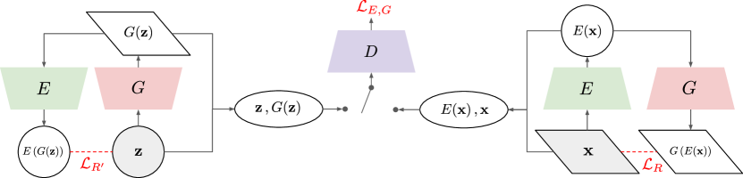
Figure 2: Overview of CBiGAN. Inputs of the model are colored in gray. Parallelograms and circles respectively represent samples in the image and latent space, while ellipses represent the inupt of the discrimintor. Red dashed lines represent the consistency loss.

We tackle anomaly detection as a one-class classification problem — we assume a training dataset $\{\mathbf{x}_{i}\}\in\mathcal{X}$ ($\mathcal{X}=\mathbb{R}^{W\times H\times C}$ for images) comprised of only non-anomalous samples. Given a test sample, we want to label it as normal/non-anomalous/defect-free (we consider it the negative class) or anomalous (positive). We rely on a GAN-based model to capture the distribution of normal data conditioned to the latent space $\mathcal{Z}=\mathbb{R}^{n}$. Similarly to [16], we adopt a BiGAN as generative model, but we instantiated it with the Wassestein distance formulation; its minimax problem is defined as

$$\min_{G,E}\max_{D}\mathbb{E}_{\mathbf{x}\sim p_{\text{data}}(\mathbf{x})}\left[{D\left(\mathbf{x},E(\mathbf{x})\right)}\right]-\mathbb{E}_{\mathbf{z}\sim p(\mathbf{z})}\left[{D\left(G(\mathbf{z}),\mathbf{z}\right)}\right]\,,$$ (4)

where $G:\mathcal{Z}\mapsto\mathcal{X}$ is the generator producing fake images from latent representations, $E:\mathcal{X}\mapsto\mathcal{Z}$ is the encoder projecting an image in its corresponding latent representation, and $D:\mathcal{X}\times\mathcal{Z}\mapsto\mathbb{R}$ is the discriminator/critic that scores samples and helps implementing the Wasserstein distance computation.

All three the modules are defined as deep neural networks and are optimized alternatively (once $G$ and $E$, once $D$) with mini-batch gradient descent. Given a mini-batch of $2N$ elements comprised of $N$ real samples $\{\mathbf{x}_{i}\}$ and $N$ randomly sampled latent representations $\{\mathbf{z}_{i}\}$, the losses for the players $\mathcal{L}_{G,E}$ and $\mathcal{L}_{D}$ are defined as

$$\mathcal{L}_{E,G}=\frac{1}{N}\sum_{i=1}^{N}D\left(\mathbf{x}_{i},E(\mathbf{x}_{i})\right)-\frac{1}{N}\sum_{i=1}^{N}D\left(G(\mathbf{z}_{i}),\mathbf{z}_{i}\right)\,,$$ (5)

and

$$\mathcal{L}_{D}=-\frac{1}{N}\sum_{i=1}^{N}D\left(\mathbf{x}_{i},E(\mathbf{x}_{i})\right)+\frac{1}{N}\sum_{i=1}^{N}D\left(G(\mathbf{z}_{i}),\mathbf{z}_{i}\right)\,.$$ (6)

Once trained on normal data, the anomaly detection procedure is reconstruction-based: given a test sample $\mathbf{x}$, we compute $E(\mathbf{x})$ to find its closest latent representation on the normal data manifold learned by the model and then compute $G\left(E(\mathbf{x})\right)$ to build its reconstruction. Following the AnoGAN approach [4], we define the anomaly score $A(\mathbf{x})$ as a linear combination of two terms: a) the pixel-based L1 reconstruction error $\mathcal{L}_{R}(\mathbf{x})$, and b) the feature-based discriminator error $\mathcal{L}_{f_{D}}(\mathbf{x})$. Formally,

$$A(\mathbf{x})=(1-\lambda)\mathcal{L}_{R}(\mathbf{x})+\lambda\mathcal{L}_{f_{D}}(\mathbf{x})\,,$$ (7)

with

$$\mathcal{L}_{R}(\mathbf{x}) =||\mathbf{x}-G\left(E(\mathbf{x})\right)||_{1}\,,$$ (8)

$$\mathcal{L}_{f_{D}}(\mathbf{x}) =||f_{D}\left(\mathbf{x},E(\mathbf{x})\right)-f_{D}\left(G\left(E(\mathbf{x})\right),E(\mathbf{x})\right)||_{1}\,,$$ (9)

where $||\cdot||_{1}$ is the $L_{1}$ norm, $f_{D}(\mathbf{x},\mathbf{z})\in\mathbb{R}^{d}$ is feature vector extracted from an intermediate output of the discriminator $D$, and $\lambda$ is a balancing hyperparameter whose value is commonly domain-specific. Intuitively, for an anomalous image both the reconstruction error $\mathcal{L}_{R}$ and the distance between discriminator features $\mathcal{L}_{f_{D}}$ increase, as the encoder $E$ usually maps the input into an out-of-distribution latent representation; therefore, the generator $G$ fails to reconstruct the input, and the discriminator $D$ extracts different representations for the original and reconstructed inputs.

Unfortunately for anomaly detection, the BiGAN training procedure does not put any constraints on $E$ and $G$ being aligned (i.e. $E^{-1}=G$ and vice-versa are not guaranteed,) and this can lead to errors and misalignment in reconstructed samples of normal data and thus to a high false positive rate. Figure 1 shows an example of this phenomenon; the reconstructed sample presents a slight rotation with respect to the input sample, and this results in an erroneous high anomaly score. To cope with this problem, we add a cycle consistency regularization term $\mathcal{L}_{C}$ to both $E$ and $G$ to promote their alignment. Formally,

$$\mathcal{L}_{C}(\mathbf{x},\mathbf{z})=\mathcal{L}_{R}(\mathbf{x})+\mathcal{L}_{R^{\prime}}(\mathbf{z})\,,$$ (10)

where

$$\mathcal{L}_{R}(\mathbf{x}) =||\mathbf{x}-G\left(E(\mathbf{x})\right)||_{1}\,\text{, and}$$ (11)

$$\mathcal{L}_{R^{\prime}}(\mathbf{z}) =||\mathbf{z}-E\left(G(\mathbf{z})\right)||_{1}\,.$$ (12)

The new loss for $E$ and $G$ is a linear combination of $\mathcal{L}_{E,G}$ and $\mathcal{L}_{C}$

$$\mathcal{L}^{*}_{E,G}=(1-\alpha)\mathcal{L}_{E,G}+\alpha\mathcal{L}_{C}\,,$$ (13)

where $\alpha$ controls the weight of each contribution. We refer to the model trained with this formulation as Consistency BiGAN (CBiGAN) whose architecture is depicted in Figure 2. Note that setting $\alpha=1$ we obtain the standard BiGAN approach (EBGAD [16]), while with $\alpha=0$ our model collapses into a non-adversarially-trained double autoencoder (on both latent and input space).

V Evaluation

V-A Dataset

	Query	Recon.	Diff.
Texture - Grid
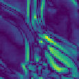
Obj. - Toothbrush

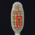
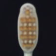
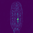
Figure 4: Examples of anomalous images from MVTec-AD (1${}^{\text{st}}$ col.), the reconstructions of our CBiGAN (2${}^{\text{nd}}$ col.), and visualization of the pixel-wise absolute difference (3${}^{\text{rd}}$ col.).

We tested and compared our approach on MVTec AD [2] — a recent real-world benchmark specifically tailored for unsupervised anomaly detection that is increasingly adopted in recent literature on this topic [27, 23, 33]. It is comprised of over 5,000 high-resolution industrial images divided into 10 objects and 5 textures categories; for each category, MVTec AD provides a training set of non-anomalous (defect-free) images and a labelled test set containing both anomalous and normal images. Details of MVTec AD are reported in Table I, and examples (together with the reconstruction performed by our model) are depicted in Figure 4.

		Train	Test		Image Side
		N	N	P
Textures	Carpet	280	28	89	1024
	Grid	264	21	57	1024
	Leather	245	32	92	1024
	Tile	230	33	84	840
	Wood	247	19	60	1024
Objects	Bottle	209	20	63	900
	Cable	224	58	92	1024
	Capsule	219	23	109	1000
	Hazelnut	391	40	70	1024
	Metal nut	220	22	93	700
	Pill	267	26	141	800
	Screw	320	41	119	1024
	Toothbrush	60	12	30	1024
	Transistor	213	60	40	1024
	Zipper	240	32	119	1024

TABLE I: MVTec-AD dataset details. N = # of negative (anomaly-free) samples. P = # of positive (anomalous) samples. All images are squared with side length given in the last column.

V-B Implementation Details

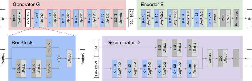
Figure 3: Our implementation of $E$, $G$, and $D$ of CBiGAN for MVTec AD. White blocks specify input and output shapes, and dark gray blocks indicate learnable convolutions (<filter_width x filter_height, num_filters>) or fully-connected layers (<num_outputs>). The negative slope of LeakyReLU activations is $0.2$. Upsampling adopts bilinear interpolation.

We follow the evaluation procedure commonly adopted in related work [4] in the unsupervised setting. We implemented $E$, $G$, and $D$ as standard residual convolutional networks. Architectural details are reported in Figure 3. We train CBiGAN separately for each category using the corresponding anomaly-free training set. Different preprocessing are adopted depending on the type of object considered:

• for ‘Object’ categories, we resize the input images to 128x128, and we apply data augmentation in the form of random rotation in the $[-45\degree,+45\degree]$ range whenever the orientation of the object is independent of its abnormality — for Bottle, Hazelnut, Metal nut, and Screw categories;

• for ‘Texture’ categories, we resize the input image to 512x512 and processed in 64x64 patches; when training, we randomly crop 64x64 patches from the input image and apply random clockwise rotation in the $[0\degree,+45\degree]$ range, and during testing, we divide the input image in 64x64 patches, derive a local anomaly score for each patch, and obtain a global score by picking the maximum local score.

For all models and categories, we use a 64-dimensional latent space ($\mathcal{Z}=\mathbb{R}^{64}$) sampled using a normal distribution. We tuned the weight of the consistency loss $\alpha$ experimentally; good values are $\alpha=10^{-4}$ for ‘Objects’ and $\alpha\in[10^{-4},10^{-5}]$ for ‘Textures’ depending on the importance of pixel-level details in detecting an anomaly. Note that small values of $\alpha$ are needed to balance the usually large values of the consistency loss term $\mathcal{L}_{C}$ that depends on the input and latent dimensions. We also produce the results for EGBAD [16] by setting $\alpha=0$. All models are trained using the Adam optimizer with a learning rate of $1e^{-4}$. Following [4], we set $\lambda=0.1$ when computing the anomaly score $A(\mathbf{x})$ for testing images.

V-C Evaluation Metrics

To quantitatively evaluate the quality of the tested approaches, for each category we compute

• the maximum Balanced Accuracy $B=\frac{\text{TPR}+\text{TNR}}{2}$ obtained when varying the threshold on the anomaly score; this is often reported by previous work [2, 27] and referred to as “the mean of the ratio of correctly classified samples of anomaly-free (TNR) and anomalous images (TPR)”. The choice of the threshold is equivalent to the maximization of the Youden’s index [34] $J=\text{TPR}+\text{TNR}-1$.

• the Area Under the ROC Curve (auROC), commonly adopted as a threshold-independent quality metric for classification.

We also report per-type and overall means of the above metrics as a unique indicator of the quality of the compared methods.

V-D Comparison with State of the Art

We compare our approaches with several methods tackling one-class anomaly detection and obtaining state-of-the-art results on MVTec AD. We divide the methods into

• iterative methods that require an iterative optimization for each sample on which anomaly detection is performed and include AnoGAN [4] and VAE-grad [19], and

• single-pass methods that perform anomaly detection in the testing phase with a single forward evaluation of the model and include AE${}_{\text{L2}}$ and AE${}_{\text{SSIM}}$ [11], AVID [26], LSA [35], EGBAD [16], GeoTrans [22], GANomaly [14], ITAE [23], and our CBiGAN.

In the latter, we also include CAVGA [27] even if the authors report results using models trained with additional data and thus not directly comparable with the other methods. For EGBAD, results are coming from our implementation, as it is generalized by CBiGAN and can be obtained with $\alpha=0$.

V-E Results

Tables V-E and V-E report results for each compared methods and for each category of MVTec AD. Compared to EGBAD, that is the approach we extend, we observe that the consistency constraint added in our model consistently improve the detection of anomalies in all the categories (with Zipper being the only exception) by at most 49%, achieving a +15% improvement on the overall balanced accuracy; the same conclusion can be drawn also from the auROC metric. These performance gains are achieved maintaining the exact same computational cost of EGBAD during prediction (a single forward pass of $E$ and $G$) and avoiding expensive iterative methods. The only additional cost to the BiGAN approach is the computation of the consistency loss $\mathcal{L}_{C}$ during the offline training phase.

Figure 5 reports some relevant examples of the differences between EGBAD and CBiGAN. Note that our higher quality of reconstructions is due to the recovered alignment and the higher color fidelity in background colors, that overall inducing smaller differences in non-anomalous areas. The Zipper class is challenging for both EGBAD and our model, as we deem the anomalous parts of the image (usually dents) are small with respect to other source of variability (the border of the zipper) that need to be modeled (see Figure 5 last row); thus both models tend to have a high reconstruction loss for both normal and anomalous samples.

Both metrics also show that CBiGAN improves on all the compared methods when dealing with textures anomalies, reaching respectively a mean balanced accuracy and mean auROC of 0.84 and 0.85 and outperforming also methods using additional data. When all categories are concerned, our method performs comparably to both other single-pass and iterative methods in terms of overall balanced accuracy, respectively obtaining a +3% (vs AVID, LSA) and -1% (vs VAE-grad) performance with respect to the second best methods.

Experiments on objects display a more complex situation; among single-pass methods, an absolute best does not emerge, and different categories benefit from specific peculiarities of each method. CBiGAN does improve on vanilla BiGAN (EGBAD) on objects, but overall, our method offers an average performance comparable or slightly degraded ($\sim$2-3%) with respect to other single-pass methods. Note that the performance of the vanilla L2 autoencoder suggests that tuning the $\alpha$ hyperparameter for each particular object category could further increase performance of CBiGAN (e.g. Zipper could benefit from a higher $\alpha$), but for sake of simplicity, we refrain from exploring class-specific parameter values in this work and prefer presenting results for fixed reasonable values. Among the few methods reporting the auROC on MVTec AD data, our model still achieves state-of-the-art performance on textures and offers a better or comparable performance with respect to other methods on objects with the only exception represented by ITAE [23] — a data-augmentation-based denoising autoencoder. At the time of writing, we abstain from discussing the performance of ITAE due to reproducibility issues.

	Textures						Objects											Overall Mean
	Carpet	Grid	Leather	Tile	Wood	Mean	Bottle	Cable	Capsule	Hazelnut	MetalNut	Pill	Screw	Toothbrush	Transistor	Zipper	Mean
Iterative methods
AnoGAN [4]†	0.49	0.51	0.52	0.51	0.68	0.54	0.69	0.53	0.58	0.50	0.50	0.62	0.35	0.57	0.67	0.59	0.56	0.55
VAE-grad [19]†	0.67	0.83	0.71	0.81	0.89	0.78	0.86	0.56	0.86	0.74	0.78	0.80	0.71	0.89	0.70	0.67	0.76	0.77
Single-pass methods
AE${}_{\text{SSIM}}$ [11]⋆	0.67	0.69	0.46	0.52	0.83	0.63	0.88	0.61	0.61	0.54	0.54	0.60	0.51	0.74	0.52	0.80	0.64	0.63
AE${}_{\text{L2}}$ [11]⋆	0.50	0.78	0.44	0.77	0.74	0.65	0.80	0.56	0.62	0.88	0.73	0.62	0.69	0.98	0.71	0.80	0.74	0.71
AVID [26]†	0.70	0.59	0.58	0.66	0.83	0.67	0.88	0.64	0.85	0.86	0.63	0.86	0.66	0.73	0.58	0.84	0.75	0.73
LSA [35]†	0.74	0.54	0.70	0.70	0.75	0.69	0.86	0.61	0.71	0.80	0.67	0.85	0.75	0.89	0.50	0.88	0.75	0.73
EGBAD [16]	0.60	0.50	0.65	0.73	0.80	0.66	0.68	0.66	0.55	0.50	0.55	0.63	0.50	0.48	0.68	0.59	0.58	0.61
CBiGAN (ours)	0.60	0.99	0.87	0.84	0.88	0.84	0.84	0.73	0.58	0.75	0.67	0.76	0.67	0.97	0.74	0.55	0.73	0.76
Methods using additional data
CAVGA-Du [27]	0.73	0.75	0.71	0.70	0.85	0.75	0.89	0.63	0.83	0.84	0.67	0.88	0.77	0.91	0.73	0.87	0.80	0.78
CAVGA-Ru [27]	0.78	0.78	0.75	0.72	0.88	0.78	0.91	0.67	0.87	0.87	0.71	0.91	0.78	0.97	0.75	0.94	0.84	0.82

TABLE II: MVTec-AD: Maximum Balanced Accuracy $B=\nicefrac{{\left(\text{TPR}+\text{TNR}\right)}}{{2}}$ when varying the anomaly score threshold for each category. The last column reports the average balanced accuracy. ^⋆Results from [2]. ^†Results from [27]. Results in boldface indicate best performing methods using only the training data provided by MVTec-AD, while underlined results indicate the best method also among the ones using additional data.

	Textures						Objects											Overall Mean
	Carpet	Grid	Leather	Tile	Wood	Mean	Bottle	Cable	Capsule	Hazelnut	MetalNut	Pill	Screw	Toothbrush	Transistor	Zipper	Mean
AE${}_{\text{L2}}^{\dagger}$	0.64	0.83	0.80	0.74	0.97	0.80	0.65	0.64	0.62	0.73	0.64	0.77	1.00	0.77	0.65	0.87	0.74	0.75
GeoTrans [22]†	0.44	0.62	0.84	0.42	0.61	0.59	0.74	0.78	0.67	0.36	0.81	0.63	0.50	0.97	0.87	0.82	0.71	0.67
GANomaly [14]†	0.70	0.71	0.84	0.79	0.83	0.77	0.89	0.76	0.73	0.79	0.70	0.74	0.75	0.65	0.79	0.75	0.76	0.76
ITAE [23]†	0.71	0.88	0.86	0.74	0.92	0.82	0.94	0.83	0.68	0.86	0.67	0.79	1.00	1.00	0.84	0.88	0.85	0.84
EGBAD [16]	0.52	0.54	0.55	0.79	0.91	0.66	0.63	0.68	0.52	0.43	0.47	0.57	0.46	0.64	0.73	0.58	0.57	0.60
CBiGAN (ours)	0.55	0.99	0.83	0.91	0.95	0.85	0.87	0.81	0.56	0.77	0.63	0.81	0.58	0.94	0.77	0.53	0.73	0.77

TABLE III: MVTec-AD: Area Under the ROC curve (auROC). ^†Results from [23]

	EGBAD [16]		CBiGAN (ours)
Query	Recon.	Diff.	Recon.	Diff.

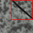
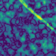
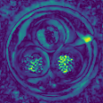
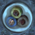
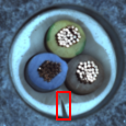
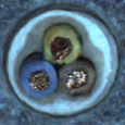
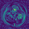
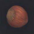
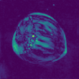
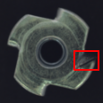
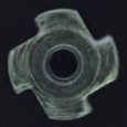
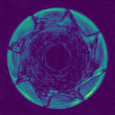
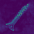
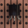
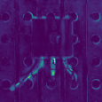
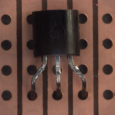
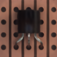
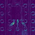
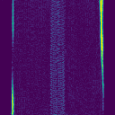
Figure 5: CBiGAN vs EGBAD — input images (1${}^{\text{st}}$ col., red boxes indicate anomalies), reconstructions (2${}^{\text{nd}}$ & 4${}^{\text{th}}$ col.), and per-pixel absolute differences (3${}^{\text{rd}}$ & 5${}^{\text{th}}$ col.). Best viewed in electronic format.

VI Conclusion

We tackled one-class anomaly detection of images using deep generative models and reconstruction-based approaches. We proposed CBiGAN — an improved Bidirectional GAN model with a consistency regularization on both the encoder and decoder modules. Our model generalizes and combines both BiGANs and Autoencoders to retain the modelling power of the former and the reconstruction accuracy of the latter. We evaluated our proposal on MVTec AD — a real-world benchmark for unsupervised visual anomaly detection with focus on industrial applications. The results of our experiments showed that our proposal greatly improves the reconstruction ability (and thus performance) of vanilla bidirectional GANs on both texture and object categories while maintaining its efficiency at test time. Our CBiGAN is particularly effective on texture-type images where it sets the new state of the art obtaining the best mean accuracy and auROC among competing methods including expensive iterative ones and approaches using additional data. Concerning object-type images, we observed that no particular method prevails on others, as each object category comes with different peculiarities. In this context, our model provides an average performance comparable with other efficient (single-pass) methods. In future work, we plan to evaluate our model also on the task of anomaly localization and gain insight on the effect of $\alpha$ in that context.

Acknowledgment

This work was partially funded by “Automatic Data and documents Analysis to enhance human-based processes” (ADA, CUP CIPE D55F17000290009) and the AI4EU project (funded by the EC, H2020 - Contract n. 825619). We gratefully acknowledge the support of NVIDIA Corporation with the donation of a Tesla K40 GPU and a Jetson TX2 used for this research.

References

- Tout et al. [2017] K. Tout, F. Retraint, and R. Cogranne, “Automatic vision system for wheel surface inspection and monitoring,” in ASNT Annual Conference 2017, 2017, pp. 207–216.
- Bergmann et al. [2019] P. Bergmann, M. Fauser, D. Sattlegger, and C. Steger, “Mvtec ad–a comprehensive real-world dataset for unsupervised anomaly detection,” in Proceedings of the IEEE Conference on Computer Vision and Pattern Recognition, 2019, pp. 9592–9600.
- Prokopetc and Bartoli [2017] K. Prokopetc and A. Bartoli, “Slim (slit lamp image mosaicing): handling reflection artifacts,” International journal of computer assisted radiology and surgery, vol. 12, no. 6, pp. 911–920, 2017.
- Schlegl et al. [2017] T. Schlegl, P. Seeböck, S. M. Waldstein, U. Schmidt-Erfurth, and G. Langs, “Unsupervised anomaly detection with generative adversarial networks to guide marker discovery,” in International conference on information processing in medical imaging. Springer, 2017, pp. 146–157.
- Yang et al. [2009] X. Yang, L. J. Latecki, and D. Pokrajac, “Outlier detection with globally optimal exemplar-based gmm,” in Proceedings of the 2009 SIAM International Conference on Data Mining. SIAM, 2009, pp. 145–154.
- Cohen et al. [2008] G. Cohen, H. Sax, A. Geissbuhler et al., “Novelty detection using one-class parzen density estimator. an application to surveillance of nosocomial infections.” in Mie, 2008, pp. 21–26.
- Radovanović et al. [2014] M. Radovanović, A. Nanopoulos, and M. Ivanović, “Reverse nearest neighbors in unsupervised distance-based outlier detection,” IEEE transactions on knowledge and data engineering, vol. 27, no. 5, pp. 1369–1382, 2014.
- Chehreghani [2016] M. H. Chehreghani, “K-nearest neighbor search and outlier detection via minimax distances,” in Proceedings of the 2016 SIAM International Conference on Data Mining. SIAM, 2016, pp. 405–413.
- Aggarwal [2015] C. C. Aggarwal, “Outlier analysis,” in Data mining. Springer, 2015, pp. 237–263.
- Manzoor et al. [2016] E. Manzoor, S. M. Milajerdi, and L. Akoglu, “Fast memory-efficient anomaly detection in streaming heterogeneous graphs,” in Proceedings of the 22nd ACM SIGKDD International Conference on Knowledge Discovery and Data Mining, 2016, pp. 1035–1044.
- Bergmann et al. [2018] P. Bergmann, S. Löwe, M. Fauser, D. Sattlegger, and C. Steger, “Improving unsupervised defect segmentation by applying structural similarity to autoencoders,” arXiv preprint arXiv:1807.02011, 2018.
- Wang et al. [2020] X. Wang, Y. Du, S. Lin, P. Cui, Y. Shen, and Y. Yang, “Advae: a self-adversarial variational autoencoder with gaussian anomaly prior knowledge for anomaly detection,” Knowledge-Based Systems, vol. 190, p. 105187, 2020.
- Schlegl et al. [2019] T. Schlegl, P. Seeböck, S. M. Waldstein, G. Langs, and U. Schmidt-Erfurth, “f-anogan: Fast unsupervised anomaly detection with generative adversarial networks,” Medical image analysis, vol. 54, pp. 30–44, 2019.
- Akcay et al. [2018] S. Akcay, A. Atapour-Abarghouei, and T. P. Breckon, “Ganomaly: Semi-supervised anomaly detection via adversarial training,” in Asian Conference on Computer Vision. Springer, 2018, pp. 622–637.
- [15] V. Dumoulin, I. Belghazi, B. Poole, A. Lamb, M. Arjovsky, O. Mastropietro, and A. C. Courville, “Adversarially learned inference,” in 5th International Conference on Learning Representations, ICLR 2017, Toulon, France, April 24-26, 2017, Conference Track Proceedings.
- Zenati et al. [2018a] H. Zenati, C. S. Foo, B. Lecouat, G. Manek, and V. R. Chandrasekhar, “Efficient gan-based anomaly detection,” arXiv preprint arXiv:1802.06222, 2018.
- Zhou and Paffenroth [2017] C. Zhou and R. C. Paffenroth, “Anomaly detection with robust deep autoencoders,” in Proceedings of the 23rd ACM SIGKDD International Conference on Knowledge Discovery and Data Mining, 2017, pp. 665–674.
- Chen et al. [2017] J. Chen, S. Sathe, C. Aggarwal, and D. Turaga, “Outlier detection with autoencoder ensembles,” in Proceedings of the 2017 SIAM international conference on data mining. SIAM, 2017, pp. 90–98.
- Dehaene et al. [2020] D. Dehaene, O. Frigo, S. Combrexelle, and P. Eline, “Iterative energy-based projection on a normal data manifold for anomaly localization,” arXiv preprint arXiv:2002.03734, 2020.
- Pawlowski et al. [2018] N. Pawlowski, M. C. Lee, M. Rajchl, S. McDonagh, E. Ferrante, K. Kamnitsas, S. Cooke, S. Stevenson, A. Khetani, T. Newman et al., “Unsupervised lesion detection in brain ct using bayesian convolutional autoencoders,” 2018.
- Zimmerer et al. [2019] D. Zimmerer, F. Isensee, J. Petersen, S. Kohl, and K. Maier-Hein, “Unsupervised anomaly localization using variational auto-encoders,” in International Conference on Medical Image Computing and Computer-Assisted Intervention. Springer, 2019, pp. 289–297.
- Golan and El-Yaniv [2018] I. Golan and R. El-Yaniv, “Deep anomaly detection using geometric transformations,” in Advances in Neural Information Processing Systems, 2018, pp. 9758–9769.
- Huang et al. [2019] C. Huang, J. Cao, F. Ye, M. Li, Y. Zhang, and C. Lu, “Inverse-transform autoencoder for anomaly detection,” arXiv preprint arXiv:1911.10676, 2019.
- Berg et al. [2019] A. Berg, J. Ahlberg, and M. Felsberg, “Unsupervised learning of anomaly detection from contaminated image data using simultaneous encoder training,” arXiv preprint arXiv:1905.11034, 2019.
- [25] J. Donahue, P. Krähenbühl, and T. Darrell, “Adversarial feature learning,” in 5th International Conference on Learning Representations, ICLR 2017, Toulon, France, April 24-26, 2017, Conference Track Proceedings.
- Sabokrou et al. [2018] M. Sabokrou, M. Pourreza, M. Fayyaz, R. Entezari, M. Fathy, J. Gall, and E. Adeli, “Avid: Adversarial visual irregularity detection,” in Asian Conference on Computer Vision. Springer, 2018, pp. 488–505.
- Venkataramanan et al. [2019] S. Venkataramanan, K.-C. Peng, R. V. Singh, and A. Mahalanobis, “Attention guided anomaly detection and localization in images,” arXiv preprint arXiv:1911.08616, 2019.
- Zenati et al. [2018b] H. Zenati, M. Romain, C.-S. Foo, B. Lecouat, and V. Chandrasekhar, “Adversarially learned anomaly detection,” in 2018 IEEE International Conference on Data Mining (ICDM). IEEE, 2018, pp. 727–736.
- Goodfellow et al. [2014] I. Goodfellow, J. Pouget-Abadie, M. Mirza, B. Xu, D. Warde-Farley, S. Ozair, A. Courville, and Y. Bengio, “Generative adversarial nets,” in Advances in neural information processing systems, 2014, pp. 2672–2680.
- Salimans et al. [2016] T. Salimans, I. Goodfellow, W. Zaremba, V. Cheung, A. Radford, and X. Chen, “Improved techniques for training gans,” in Advances in neural information processing systems, 2016, pp. 2234–2242.
- Arjovsky et al. [2017] M. Arjovsky, S. Chintala, and L. Bottou, “Wasserstein generative adversarial networks,” in Proceedings of the 34th International Conference on Machine Learning, ICML 2017, Sydney, NSW, Australia, 6-11 August 2017, ser. Proceedings of Machine Learning Research, D. Precup and Y. W. Teh, Eds., vol. 70. PMLR, 2017, pp. 214–223. [Online]. Available: http://proceedings.mlr.press/v70/arjovsky17a.html
- Gulrajani et al. [2017] I. Gulrajani, F. Ahmed, M. Arjovsky, V. Dumoulin, and A. C. Courville, “Improved training of wasserstein gans,” in Advances in neural information processing systems, 2017, pp. 5767–5777.
- Liu et al. [2019] W. Liu, R. Li, M. Zheng, S. Karanam, Z. Wu, B. Bhanu, R. J. Radke, and O. Camps, “Towards visually explaining variational autoencoders,” arXiv preprint arXiv:1911.07389, 2019.
- Sokolova et al. [2006] M. Sokolova, N. Japkowicz, and S. Szpakowicz, “Beyond accuracy, f-score and roc: a family of discriminant measures for performance evaluation,” in Australasian joint conference on artificial intelligence. Springer, 2006, pp. 1015–1021.
- Abati et al. [2019] D. Abati, A. Porrello, S. Calderara, and R. Cucchiara, “Latent space autoregression for novelty detection,” in Proceedings of the IEEE Conference on Computer Vision and Pattern Recognition, 2019, pp. 481–490.