Data-driven quantitative modeling of bacterial active nematics

Abstract

Active matter comprises individual units that convert energy into mechanical motion. In many examples, such as bacterial systems and biofilament assays, constituent units are elongated and can give rise to local nematic orientational order. Such ‘active nematics’ systems have attracted much attention from both theorists and experimentalists. However, despite intense research efforts, data-driven quantitative modeling has not been achieved, a situation mainly due to the lack of systematic experimental data and to the large number of parameters of current models. Here we introduce a new active nematics system made of swarming filamentous bacteria. We simultaneously measure orientation and velocity fields and show that the complex spatiotemporal dynamics of our system can be quantitatively reproduced by a new type of microscopic model for active suspensions whose important parameters are all estimated from comprehensive experimental data. This provides unprecedented access to key effective parameters and mechanisms governing active nematics. Our approach is applicable to different types of dense suspensions and shows a path towards more quantitative active matter research.

This manuscript was compiled on

Examples of active matter can be found at diverse lengthscales (1, 2, 3, 4, 5, 6) from animal groups (7, 8, 9, 10, 11) to cell colonies and tissues (12, 13, 14, 15, 16, 17, 18), to in vitro cytoskeletal extracts (19, 20, 21, 22, 23, 24, 25, 23, 26), and man-made microscopic objects (27, 28, 29, 30, 31, 32). Energy input at the level of the individual constituents drives active matter systems out of thermal equilibrium and leads to a wide range of collective phenomena, including flocking (7, 28, 29, 33, 19, 34), swarming (12, 13), clustering (27, 14, 30, 32), two-dimensional long-range order (35, 15), giant number fluctuations (35, 15, 36, 33, 14), spontaneous flow (37, 38, 21, 24, 25), and synchronization (16).

Active matter systems consisting of elongated particles often lead to local nematic orientational order. This important active nematics class comprises experiments with vibrating granular rods (36), crawling cells (39, 40, 41), swarming sperms (42), filamentous bacteria (15) and motor-driven microtubules (21, 20, 24), which, together with theoretical work, have shown that the interplay between orientational order, active stress, particle and fluid flow leads to complex spatial-temporal dynamics and unusual fluctuations. The seminal work by the group of Dogic (21, 43) has been particularly influential. They experimentally observed spontaneous chaotic dynamics driven by topological defects, and their results triggered a large number of theoretical and modeling approaches. These are of two main types, particle-level ‘microscopic’ models (44, 45, 43) and continuous-level ‘hydrodynamic’ descriptions (46, 47, 48, 49, 50, 51, 52, 53), with the latter usually written phenomenologically or by complementing equilibrium liquid crystal theories with minimal active terms. These studies provided important insights into the multi-faceted dynamics of active nematics, such as hydrodynamic instabilities, long-range correlations, anomalous fluctuations, defect dynamics, spatial and temporal chaos. However, these models generally contain a large number of parameters. This has made comparisons between models and experiments semi-quantitative at best.

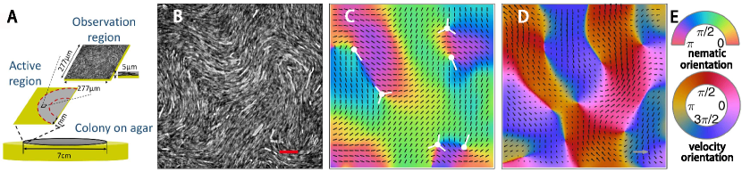
Figure 1: (A) Schematic illustration of a bacteria colony growing on agar; the active nematics dynamics studied here takes place in a millimeter-wide, few-micron thick region at the edge; our observation region is typically $277\times 277\mu{\rm m}$. Mean cell length varies from $6$ to $14\mu m$, depending on antibiotic concentration. (B) raw image of our fluorescent cells (scale bar 30$\mu m$) in some experiment performed at 45 $\mu g/mL$ drug level. (C,D) nematic order and velocity fields extracted from B. Black rods in C represent unit length director vector $\hat{\bf u}$, and length of arrows in D is proportional to the local speed (scale bar 250 $\mu m/s$). (E): colormaps coding the orientation of the nematic and velocity fields in C and D. The white symbols in C represent the $\pm\frac{1}{2}$ defects (see SI text and Fig. S2 for details about their orientation).

Bacteria are widely used as model systems to study active matter (12, 13, 14, 15, 16). A recent study showed that elongated E. coli cells strongly confined between two glass plates can display the long-range nematic order and anomalous fluctuations typical of dry, dilute active nematics systems (15). However, so far, almost no bacterial system has been reported to exhibit the phenomenology of dense, wet active nematics as reported first by Dogic et al.. One exception is a study of motile bacteria dispersed in a nontoxic lyotropic nematic liquid crystal (54, 55). When bacteria concentration is high enough, active stress destabilizes the ordered nematic state of this biosynthetic system, leading to a state where topological defects in the liquid crystal evolve chaotically in a manner closely resembling that of the Dogic system. Here, we show that the typical phenomenology of wet, dense, active nematics can be experimentally realized in colonies of filamentous bacteria and show how to build a data-driven quantitatively-faithful theoretical description of it. To this aim, we introduce a new type of microscopic model for active suspensions and we use simultaneous experimental measurements of both orientation and velocity fields to estimate all its parameters.

Experimental results

Our experiments are carried out with Serratia marcescens bacteria. At the edge of growing colonies, 2-3 layers of cells actively swim by rotating flagella in a micrometer-thick millimeters-wide film of liquid on the agar surface (Fig. 1A). Apart from a narrow ($\sim 100\mu$m) outer ring, the thickness of this quasi-2D suspension is very constant. No obvious spatial or temporal inhomogeneity is noticeable in measured fields. A sub-lethal level of antibiotic drug Cephalexin is added into the growth agar medium. The drug allows bacteria to grow but not to divide, leading to long cells. By varying the drug concentration, we can change the mean cell length by a factor of two, see Fig. S1A. Bacteria are labeled with a green fluorescent protein, which allows to record their motion under the microscope. In the dense, thin layer of interest, cells are almost always in close contact and nearly cover the whole surface. Our elongated cells are also frequently nematically aligned, as testified by the presence of $\pm\frac{1}{2}$ charge topological defects typical of 2D nematics (Fig. 1B). (Standard cells cultivated without antibiotic drug do not give rise to any significant local order.) Our images do not allow to distinguish the current polarity of each cell, i.e. in which direction it is currently swimming with respect to the fluid. In fact, the swimming of most bacteria is strongly hampered at such high density. Nevertheless, our cells move collectively, mainly advected by the fluid they have set in motion, in a spatiotemporally chaotic manner strongly reminiscent of other active nematics systems (21, 54) (Movies S1 and S2). From each image, we extract a nematic orientation field $\hat{\bf u}({\bf r},t)$ through a gradient-based method, and ${\bf v}({\bf r},t)$ the velocity field of cells in the laboratory frame using a standard particle image velocimetry technique (Fig. 1C,D, SI Appendix, Fig. S2). Movie S1 shows the typical evolution of the obtained coarse-grained orientation and velocity fields. This dynamics is fast. Typical correlation times are of the order of seconds (see below). In each experiment, we record images for 30 s, which is significantly shorter than the cell division time (20 min). Therefore, contributions of cell growth to active stress are negligible in our work (56, 57).

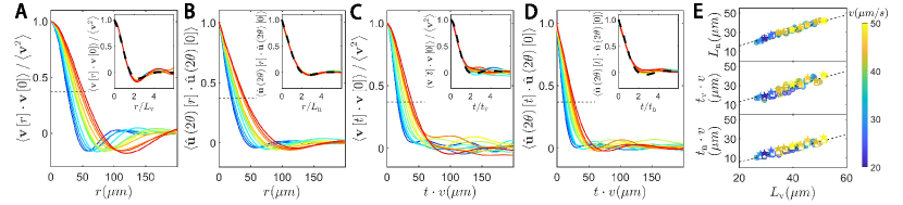
Figure 2: Spatial (A and B) and temporal (C and D) two-point correlation functions (defined in y-axis labels) from experiments with drug concentrations from 30$\mu g/mL$ to 60$\mu g/mL$. The color of each curve codes for the velocity correlation length $L_{\rm v}$. Insets: correlation functions rescaled by their correlation length/time. Dashed lines: correlation functions calculated from numerical simulations of the model performed at the optimal-match parameter values estimated for the typical 45 $\mu g/mL$ experiment shown in Fig. 1, corresponding to 6th column in SI Appendix, Table S1. (E): variation of various correlation lengths with the velocity correlation length $L_{\rm v}$ for both experiments (solid circles and open squares) and simulations of our model at optimal parameter values (solid stars). The experiments noted by open squares are those corresponding to the optimal model simulations noted with solid stars. Each symbol is colored according to the mean speed $v$ measured (colormap at the right).

Global measurements

We first measure global statistical properties of our velocity and orientation fields. The average cell speed $v\equiv\langle|{\bf v}({\bf r},t)|\rangle_{{\bf r},t}$ varies between 20 and $50\text{ }\mu m/s$ from experiment to experiment but is approximately independent of the drug concentration (SI Appendix, Fig. S1B,C).

Next we compute spatial and temporal two-point correlation functions, which are defined and shown in Fig. 2A-D. The spatial/temporal separations corresponding to a correlation value of $1/e$ are identified as the correlation lengths and times. Symbols $L_{\rm v}$, $L_{\rm n}$, $t_{\rm v}$, and $t_{\rm n}$ respectively denote velocity and orientation correlation lengths, velocity and orientation correlation times. These quantities are typically of the order of tens of $\mu m$ and one second. When we increase the cell length with antibiotics, the correlation lengths $L_{\rm n}$ and $L_{\rm v}$ increase systematically (Fig. 2A,B). Such a systematic variation is only observed for correlation times $t_{\rm n}$ and $t_{\rm v}$ if time is rescaled by the mean speed $v$ (Fig. 2C,D). Correlation functions from various experiments with different drug concentrations collapse onto each other when space and time are rescaled by correlation lengths and times (insets in Fig. 2A-D). Moreover, all these quantities are linearly related to each other. Strikingly, transforming correlation times into correlation lengths using the mean speed $v$, we find that $L_{\rm n}$, $v\cdot t_{\rm n}$, and $v\cdot t_{\rm v}$ are all proportional to $L_{\rm v}$ with approximately the same slope (Fig. 2E). This indicates that our experiments are characterized by a single lengthscale and the mean flow speed (58, 59). Because our bacteria are too closely packed to measure their length, we use $L_{\rm v}$ and $v$ as “effective control parameters” of our experiments, with $L_{\rm v}$ serving as a good proxy to the mean cell length, see SI Appendix, Fig. S1.

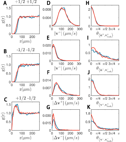
Figure 3: Statistical properties of defect cores. Experimental data extracted from the experiment at drug level 45$\mu g/mL$ that gives a correlation length $L_{\rm v}=39.7\mu m$ and a mean flow speed $v=50.4\mu m/s$ used in most of the text (blue curves), and from simulations of our model at parameter values optimized for that experiment (red curves), corresponding to 6th column of SI Appendix, Table S1. (A-C): Two-point pair correlation functions $g(r)$ for the positions of defect cores (respectively $(+\frac{1}{2},+\frac{1}{2})$, $(-\frac{1}{2},-\frac{1}{2})$, and $(+\frac{1}{2},-\frac{1}{2})$ pairs). (D-G): probability distribution functions of various defect speeds (respectively speed of $+\frac{1}{2}$ and $-\frac{1}{2}$ defects in lab frame, and speed of $+\frac{1}{2}$ and $-\frac{1}{2}$ defects in fluid frame). (H,I): probability distribution functions of angle between defect orientations $\hat{\bf u}^{\pm}$ and fluid velocity at their core ${\bf v}^{\pm}_{\rm back}$. (J,K): same as (H,I), but for the defect core velocities in the lab frame ${\bf v}^{\pm}$.

Defect properties

To go beyond the reduction of the complex spatiotemporal dynamics of our bacterial system to just a lengthscale and the mean speed, we now focus on the $\pm\frac{1}{2}$ topological defects of the orientation field. Their detailed structure and their dynamics offer unique access to the coupling between nematic order and flow, all information that we will show later to be crucial to determine model parameters.

We identify the location of $\pm\frac{1}{2}$ defects by contour integral of the director field (see Fig. 1C and Movie S1 for typical results). From the trajectories of defect cores, we measure ${\bf v}^{\pm}$, their velocity in the lab frame. We also measured the velocity of defects in the fluid frame, $\Delta{\bf v}^{\pm}={\bf v}^{\pm}-{\bf v}^{\pm}_{\rm back}$, where ${\bf v}^{\pm}_{\rm back}$ is the fluid “backflow” velocity averaged over a small region surrounding the defect core (see SI Appendix, Fig. S2D). We finally determine the intrinsic orientation $\hat{\bf u}^{\pm}$ of defects. This is straightforward for the comet-shaped $+\frac{1}{2}$ defects. For the $-\frac{1}{2}$ defects, which are not polar but have a three-fold symmetry with three radial axes along which the nematic director is aligned, we choose the axis closest to the current orientation of ${\bf v}^{-}$ (see SI Appendix and SI Appendix, Fig. S2 for details).

As in other active nematics systems (36, 21, 41), defects are created in $\pm$ pairs via the bending of ordered regions (Movie S1). Upon generation, $+\frac{1}{2}$ defects typically quickly move away and less motile $-\frac{1}{2}$ defects stay longer near the generation site. Pair of defects of opposite charge may also annihilate upon encounter. In a given experiment, generation and annihilation of defects balance each other so that their total number is approximately constant in time. The radial distribution functions of defect position, $g\left(r\right)$, reveals that defects with the same sign repel from each other at short distances (Fig. 3A-C). For defects of opposite sign, $g(r)$ has a short-scale peak reflecting the fact that defects are created in $\pm$ pairs (43).

Restricting our analysis to “isolated” defects from now on, i.e. whose distance from nearest neighbors is larger than nematic correlation length $L_{\rm n}$, we observe that they are essentially distributed randomly in space: no global translational nor orientational order is observed. Defect speed distributions, both in the lab and in the fluid frame, show that $+\frac{1}{2}$ defects are more motile, but $-\frac{1}{2}$ defects do not have a negligible speed, even in the fluid frame (Fig. 3E,G). We also find that the defect orientation $\hat{\bf u}^{\pm}$ is strongly correlated to their velocity orientation, and to the orientation of their velocity in the fluid frame. Essentially, all three vectors are aligned, even for the $-\frac{1}{2}$ defects (Fig. 3H-K). Note that a small but finite velocity in the fluid frame $\Delta{\bf v}^{-}$ is at odds with usual statements about $-\frac{1}{2}$ defects in active nematics, where they are treated as symmetric, force-free, diffusive objects (60, 53, 44). We elaborate on this point in Discussion section.

To further quantify the structure of defects, we average, over time and many defects, the orientation and velocity fields around their core, sitting in their intrinsic reference frame. The familiar mushroom-shape and three-fold symmetry of, respectively, the $+\frac{1}{2}$ and $-\frac{1}{2}$ defect are clearly observed (Fig. 4A,B). The flow field around the $+\frac{1}{2}$ defect core shows a strong jet, while 3 nearly symmetric jets go through the center of the $-\frac{1}{2}$ defect (Fig. 4C,D), in agreement with previous work (60, 53).

Because of the chaotic collective dynamics, the magnitude of these averaged fields decays away from the defect core. We define defect core sizes $R^{\pm}$ as the radius where the magnitude of averaged director vector $\left|\textrm{u}_{\rm a}\right|$ reaches value $\frac{1}{2}$. For the quantitative modeling of our system, we also extracted angular profiles of orientation and velocity around defect cores from the averaged fields. In Fig. 4E,F, we plot profiles of the angle of the nematic director calculated at three different radii around the defect cores. These profiles show clear systematic deviations from the linear variation predicted in one-constant equilibrium liquid crystals theory (61). The velocity orientation profiles, as well as the profiles of the magnitude of orientation and velocity fields show also systematic variations reflecting the fine-structure of defects (Fig. 4I-L).

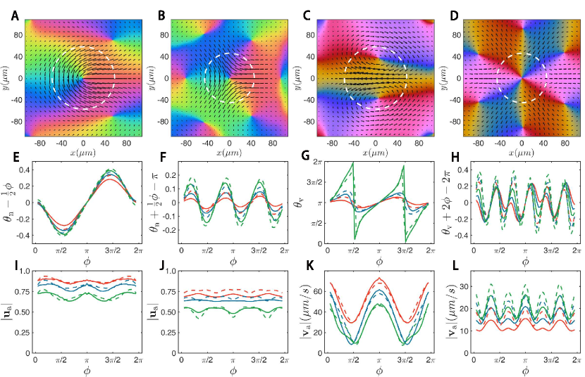
Figure 4: Mean nematic (columns 1 & 2) and velocity (columns 3 & 4) fields around isolated $+\frac{1}{2}$ (columns 1 & 3) and $-\frac{1}{2}$ (columns 2 & 4) defects. (A-D): full 2D representation as in Fig. 1. The white circles show the defect sizes $R^{+}$ and $R^{-}$ defined in the text. Panels in the second (E-H) and third (I-L) rows contain angular profiles of the 2D fields measured at three different radii: $23\mu m$ (red), $33\mu m$ (blue), $43\mu m$ (green). Angle $\phi$ is the angle depicting the circles of various radii around the defect cores. Mean director $\theta_{\rm n}$ and velocity $\theta_{\rm v}$ angles are defined as the angles between mean director/velocity vectors and x axis. The reference linear component ($\frac{1}{2}\phi$ in E, $\pi-\frac{1}{2}\phi$ in F, $2\pi-2\phi$ in H) has been substracted in the orientation profiles to emphasize deviations from single-Frank constant liquid crystal theory. Solid lines: angular profiles from experiments. Dashed lines in E-L: angular profiles from simulations performed at optimal parameters.

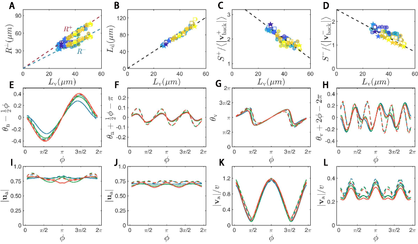
Figure 5: Dependence of defects properties on experimental conditions. (A-D): variation with nematic correlation length $L_{\rm v}$ of defect core size $R^{\pm}$ (A), mean inter-defect lengthscale $L_{\rm d}$ (B), mean of $+\frac{1}{2}$ and $-\frac{1}{2}$ defect speed $S^{\pm}$ divided by local flow speed $\left<|{\bf v}^{\pm}_{\rm back}|\right>$ (C,D). Experiment and simulation results are shown by open squares and solid stars, color-coded by the mean speed $v$, following Fig. 2E. All experiments and simulations collapse onto single straight lines, indicating that $v$ does not influence the quantities represented. (E-L) angular profiles as in Fig. 4 calculated along the circle of radius 0.6$R^{\pm}$ for 3 experimental datasets obtained at different drug levels (blue: 30$\mu g/mL$, 1st column in SI Appendix,Table S1, green: 45$\mu g/mL$, 6th column in SI Appendix, Table S1, red: 60$\mu g/mL$,12th column in SI Appendix, Table S1). Corresponding simulation results are shown using dashed lines.

We have performed the above analysis of the dynamics and fine structure of defects on a large set of experiments. We now describe how the main defect properties vary with our two effective control parameters, the correlation length $L_{\rm v}$ and the mean flow speed $v$. The defect core sizes $R^{\pm}$ vary linearly with $L_{\rm v}$, and are roughly independent of $v$ (Fig. 5A). In the steady-state, the density of defects is statistically constant. From this steady density one can extract an inter-defect lengthscale $L_{\rm d}$, which behaves like all other correlation lengths, in agreement with previous work on wet active nematics (62, 63) (Fig. 5B). We also find that the speed of defects relative to the local flow speed at their core decreases with $L_{\rm v}$ while being also roughly independent of $v$ (Fig. 5C,D, see a discussion of this below). Remarkably, the detailed spatial structure of defects does not vary significantly between experiments with different characteristic lengths: after rescaling spatial coordinates by defect core size, or, equivalently, correlation length, averaged director and velocity fields from different datasets overlap nicely. We further confirm this by comparing defect angular profiles at 0.6$R_{\pm}$ for different experiments (Figs. 5E-L).

Quantitative modeling

A microscopically faithful model of our dense, thin bacterial system where cells and their many flagella are in constant contact with each other and with the gel substrate is a formidable task well-beyond current numerical power. Besides, this would require the knowledge of many specific details that are unknown. Here we adopt a radically different approach: we treat the collisions and local interactions between cell bodies and their flagella at some effective level, where, we assume, they amount to a combination of steric repulsion and alignment. In addition, the far-field interactions and other effects due to the incompressible fluid surrounding bacteria are taken into account by solving the Stokes equation for the fluid flow. All this also allows us to build an efficient, streamlined, but comprehensive model in two space dimensions.

Description of the numerical model

Recall that most cells in our dense system are not able to swim freely, simply because nearby cells prevent them to do so (see Movie S2). These crowded cells mostly exert force dipoles on the fluid, which is then set in motion by their collective action. Cells, in turn, are advected and rotated by the fluid. Our model thus consists of non-swimming force dipoles immersed in an incompressible fluid film, and differs significantly from the common choice of using a dynamic equation for a director field (64, 65, 66, 67, 68, 69). As shown by a schematic diagram in SI Appendix, Fig. S3, each dipole represents the local cell body orientation and active forcing.

The fluid flow ${\bf v}({\bf r},t)$ is the solution of the (2D) Stokes equation

$$\mu\nabla^{2}{\bf v}+\nabla p-\alpha{\bf v}+{\bf F}=0\;\;{\rm with}\;\;\nabla\cdot{\bf v}=0$$ (1)

where $\mu$ is the fluid viscosity, $\alpha$ is the effective friction with the substrate, $p$ is the pressure enforcing the incompressibility condition, and ${\bf F}$ is the active force field exerted by dipoles on the fluid (64).

Our dipoles are point particles with position $\mathbf{r}_{i}$ and orientation $\theta_{i}$ (or, equivalently, unit orientation vector $\hat{{\bf u}}_{i}=(\cos(\theta_{i}),\sin(\theta_{i}))$. They locally align, are advected and rotated by the flow, and experience pairwise repulsion to keep their density homogeneous:

$$\dot{{\mathbf{r}}}_{i} = {\bf v}\left({\mathbf{r}}_{i}\right)+C_{\rm r}\sum_{j\sim i}{\bf R}_{ij}$$ (2)

$$\dot{\theta}_{i} = C_{\rm a}\sum_{j\sim i}\sin\left[2\left(\theta_{j}-\theta_{i}\right)\right]+C_{\rm v}\left(\nabla\times{\bf v}\right)\cdot\hat{{\bf z}}$$ (3)

$$+C_{\rm s}\hat{{\bf u}}_{i}\times\left({\bf E}\cdot\hat{{\bf u}}_{i}\right)\cdot\hat{{\bf z}}+C_{\rm n}\xi_{\theta},$$

In (3), the first term on the right-hand side, with strength $C_{\rm a}$, codes for the nematic alignment of dipole $i$ with all neighbors currently present within distance $R_{\rm a}$. The next two terms govern how dipoles are rotated by the flow field ${\bf v}$, following Jeffery’s classic work: both local vorticity $\nabla\times{\bf v}$ and local strain ${\bf E}=\left(\nabla{\bf v}+\nabla{\bf v}^{T}\right)/2$ are playing a role, but with coefficients $C_{\rm v}$ and $C_{\rm s}$ taking values a priori different from the classic ones calculated for perfect ellipsoids with no-slip boundaries (70). Finally, $\xi_{\theta}$ is a unit-variance, white, angular Gaussian noise. In (2), the right-hand side term ${\bf R}_{ij}$ represents a unit-range pairwise soft repulsion force between dipoles of strength $C_{\rm r}$. Note that self-propulsion is not included in (2) because our system is crowded.

The force field ${\bf F}$ in (1) is assumed to be dominated by the gradient of the active stress tensor field. (A small, residual contribution from the short-range repulsion force between neighboring dipoles exists, but can usually be neglected, see SI Appendix, Eq. S2 for details about this point.) The active stress tensor is itself assumed, as usual in wet active nematics studies (50, 51), to be proportional to the gradient of the orientation field:

$${\bf F}=f_{0}\nabla\cdot\hat{{\bf u}}\hat{{\bf u}}$$ (4)

where $f_{0}$ is the typical strength of dipoles. In experiments, $\hat{{\bf u}}$ is the measured nematic orientation field. In the model, $\hat{{\bf u}}$ is the local coarse-grained orientation of our dipoles.

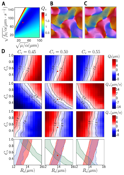
Figure 6: Quality functions and results from hydrodynamic (A-C) and full (D) model matching. Optimal parameters are marked by a red dot. (A): quality function $Q_{\rm v}$ in the $(\sqrt{\mu/\alpha},\sqrt{f_{0}/\alpha})$ plane. (B): a typical instantaneous experimental velocity field. (C): velocity field reconstructed from the orientation field measured at the same time as (B) at the optimal parameters indicated in (A). The first three rows of (D) contain quality functions of characteristic length ($Q_{\rm l}$), +1/2 defect speed ($Q_{+}$) and -1/2 defect speed ($Q_{-}$). Each panel represent a scan in the $C_{\rm s}$-$R_{\rm a}$ plane and panels in the same column use the same $C_{V}$ value. Black contour lines mark regions of acceptable deviations. Panels in the last row contain acceptable regions of parameters extracted from quality functions: red from $Q_{\rm l}$, green from $Q_{+}$ and blue from $Q_{-}$; they show that $C_{\rm v}=0.5$ yields largest overlap area for acceptable regions of parameters and a red dot in the middle panels marks the optimal choice for parameters $C_{\rm s}$ and $R_{\rm a}$.

The full system constituted by Eqs. [1-4] can be seen as a minimal Vicsek-style model (71, 72) incorporating the main mechanisms at play in our bacterial active nematics. One thus expects a basic interplay between alignment and noise: if the alignment strength $C_{\rm a}$, or the alignment range $R_{\rm a}$, or the number density of dipoles $\rho_{0}$ is large enough, or if the noise strength $C_{\rm n}$ is weak enough, local orientational (nematic) order can emerge. The global number density of dipoles $\rho_{0}$ and the noise strength $C_{\rm n}$ have opposite effects. We checked that changing $\rho_{0}$ in the experimentally reasonable range $[1.5,4]$ (in simulation units) yields similar results. In the following, we fix $\rho_{0}=1.5$ to lighten the numerical task.

It is relatively easy to find parameter values such that the dynamics of our model closely resembles the experimental observations. As a matter of fact, the region of parameter space where spatiotemporally chaotic active nematics behavior occurs is rather large. To go beyond such qualitative agreement, we have systematically investigated the effects of parameters. We now show that for each experimental dataset, there exists a unique set of parameter values at which the model optimally matches the experiment, in the sense that all quantities studied in the previous section are in quantitative agreement.

Data-driven parameter optimization

We proceed in two steps. First, simultaneous measurements of velocity and orientation fields allow us to pinpoint the parameters in (1) without resorting to the "microscopic" part of the model, i.e. Eqs. [2,3].

Dividing both sides of (1) by $\alpha$, we are left with two independent parameters, $\mu/\alpha$ and $f_{0}/\alpha$. Therefore, for any given pair of parameters $\mu/\alpha$ and $f_{0}/\alpha$, and a particular experimentally-measured orientation field $\hat{{\bf u}}$, we can compute the velocity field ${\bf v}_{*}$ solution of (1). We then compare ${\bf v}_{*}$ with ${\bf v}$, the velocity field measured at the same time as $\hat{{\bf u}}$. Scanning the whole $(\mu/\alpha,f_{0}/\alpha)$ parameter plane, we find that there is an optimal point where the difference between ${\bf v}_{*}$ and ${\bf v}$ is minimal on average. Specifically, we measure the quality function $Q_{\rm v}(\mu/\alpha,f_{0}/\alpha)=\langle|{\bf v}_{*}({\bf r},t)-{\bf v}({\bf r},t)|^{2}/|{\bf v}({\bf r},t)|^{2}\rangle_{{\bf r},t},$ where the average is carried out over both space and time. A typical result for an experiment with 45$\mu g/mL$ drug concentration is in Fig. 6A, where $Q_{\rm v}$ shows a minimum for $Q_{\rm v}=0.23$ at $f_{0}/\alpha=6174\mu m^{2}/s$ and $\sqrt{\mu/\alpha}=36\mu m$. Typical instantaneous velocity fields ${\bf v}_{*}$ produced at these parameters compare very well to the corresponding ${\bf v}$ fields (Fig. 6B,C, movie S3).

After fluid parameters are fixed, we proceed to the second step and match the full model with experiments. Eqs. (2-3) contain six parameters. We first evaluate their influence by varying them individually around a reference point (see SI Appendix, and SI Appendix, Fig. S4 for details). We find that angular noise level $C_{\rm n}$ and repulsion strength $C_{\rm r}$ are not sensitive parameters provided local order is not destroyed by strong noise and particles do not crystallize for too-strong repulsion. We therefore fix $C_{\rm n}=1.0$ and $C_{\rm r}=0.5$. Nematic alignment parameters $C_{\rm a}$ and $R_{\rm a}$ play a major, but similar role, so we decide to fix $C_{\rm a}=0.4{\rm s}^{-1}$ and vary $R_{\rm a}$, mimicking the change of cell length in experiments. This leaves us with only three parameters to vary, $R_{\rm a}$, $C_{\rm v}$, and $C_{\rm s}$, when looking for an optimal match between model and experiment.

We performed a systematic scan of this restricted parameter space, running the model for many sets of parameter values, and extracting from each of these runs the quantities of interest, i.e. those measured also in the experiment. To quantify the match between model and experiment, we found that using 3 independent quality functions is sufficient. Here we use $Q_{\rm l}\equiv L_{\rm n*}-L_{\rm n}$, the difference in nematic correlation length, $Q_{+}\equiv S_{*}^{+}-S^{+}$ and $Q_{-}\equiv S^{-}_{*}-S^{-}$ the differences in defect speed ($S^{\pm}\equiv\langle|{\bf v}^{\pm}|\rangle$), respectively for the $+\frac{1}{2}$ and $-\frac{1}{2}$ defects. (As before, the $*$ subscript denotes quantities measured on the model.) Computed quality functions in the three-dimensional parameter space {$R_{\rm a}$, $C_{\rm v}$, $C_{\rm s}$} are shown in Fig. 6D. Perfect matching ($Q_{\{\rm l,+,-\}}=0$) occurs for each function on a surface. These three surfaces approximately cross at a single point, as shown in the last row of Fig. 6D. For the particular experiment considered, we find $R_{\rm a}=13.8\mu m$, $C_{\rm v}=0.5$, and $C_{\rm s}=0.5$, which thus defines our optimal set of model parameters. By construction, these parameter values optimize the match between model and experiment for what concerns the quantities involved in the quality functions used. Remarkably, we observe that all other quantities not used in these functions are also quantitatively matched. This is in particular the case for all correlation functions in Fig. 2, all distributions of defect speed and orientation, and spatial distributions of defects in Fig. 3, all averaged angular profiles of isolated defects in Fig. 4, defect size and speed in Fig. 5 (see also simulations of the model at optimal parameters in Movie S4).

Finally, we performed two "consistency checks". We verified that choosing a different value of $C_{\rm a}$ yields a different optimal value of $R_{\rm a}$ but that all other optimal parameter values then approximately remain the same (SI Appendix, Fig. S6). In short, $R_{\rm a}$ and $C_{\rm a}$ are fully redundant. Next, taking our optimal parameter set, but now “freeing” the fluid parameters $\mu/\alpha$ and $f_{0}/\alpha$ from the values determined during our first step, we find that these initial values remain optimal (SI Appendix, Fig. S7). This confirms that our procedure, for a given experiment, yields a unique set of model parameters at which model dynamics optimally matches spatiotemporal data.

Variation of model parameters

We have successfully applied our matching procedure to a large set of experiments with drug concentration above 15 $\mu g/mL$, the level below which cells are too short to give rise to a clear local nematic orientation that can be reliably measured. For each experiment, the quality of the matching between experiments and simulations remains excellent. Corresponding orientation and velocity fields from simulations at these optimal parameters are shown in Movie S4. We thus obtained the variation of the optimal model parameter values with the two experimental effective control parameters, the correlation length (proxy for cell size) and the mean flow speed $v$ (see Fig. 7 and SI Appendix, Table S1). This provides us with a wealth of information about our experimental system.

We first discuss the effect of the mean speed $v$ at fixed correlation length. Choosing a subset of experiments yielding approximately the same correlation length, we observe that $v$ almost exclusively influences $f_{0}$, and does so linearly (Fig. 7A). The other parameters remain constant with the exception of the interaction range $R_{\rm a}$, which grows slightly with $v$ (Fig. 7B-E). The clear linear growth of $f_{0}$ confirms that, via $v$, one has direct access to the the strength of forces dipoles, which, in turn, can be interpreted to be proportional to the power developed on average by each flagellum. As for the weaker linear variation of $R_{\rm a}$ with $v$, we attribute it to the fact that for higher $v$, which corresponds to higher $f_{0}$, the fluid flow would be destabilized faster, leading to a smaller correlation length. Increasing $R_{\rm a}$ compensates for this.

The variation of optimal model parameters with correlation length, at fixed mean speed $v$, is presented in Fig. 7F-J. From the extracted “fluid” parameters, we can construct two length scales that are proportional to $L_{\rm v}$. Balancing the active force term $\nabla\cdot\left(f_{0}\hat{{\bf u}}\hat{{\bf u}}\right)$ in (1) with the friction term $\alpha{\bf v}$, we have $f_{0}/(\alpha\left|{\bf v}\right|)\sim L_{\rm n}$ which leads to $f_{0}/(\alpha\left|{\bf v}\right|)\sim L_{\rm v}$. This is confirmed in Fig. 7F. We can also balance friction with the viscous force $\mu\nabla^{2}{\bf v}$ and get $\sqrt{\mu/\alpha}\sim L_{\rm n}$, as shown in Fig. 7G. (We show that the two scalings above are verified for all our data points in SI Appendix, Fig. S8.) These findings provide a physical understanding of the factors contributing to the correlation length, and in particular of how it is connected to the fluid effective parameters. The vorticity coupling parameter $C_{\rm v}$ is approximately a constant, $C_{\rm v}\simeq 0.5$ (Fig. 7H). This is in agreement with Jeffery’s theory, which shows that $C_{\rm v}=\frac{1}{2}$ for almost any axisymmetric shape from needles to ellipsoids to disks. Nearly constant $C_{\rm v}$ is also consistent with observations that defect shape changes little in different experiments (Fig. 5E-L) and that $C_{\rm v}$ is closely connected to defect shape in our model (SI Appendix, Fig. S5). On the other hand, the strain coupling parameter $C_{\rm s}$ decreases with $L_{\rm v}$ (Fig. 7I), at odds with Jeffery’s results, which show that longer objects have higher $C_{\rm s}$. This can be understood by noticing that in the model particles do not represent cells. Rather, over the interaction range $R_{\rm a}$, several dipoles stand for a cell. They react individually to the local strain, and thus their response must be weaker than that of a cell, and the longer the cell, the weaker the response. Finally, the range of nematic alignment $R_{\rm a}\sim\sqrt{L_{\rm v}}$ (Fig. 7J), which shows that the correlation length increases linearly with the area where nematic alignment takes place, i.e the number of aligning neighbors, in our model.

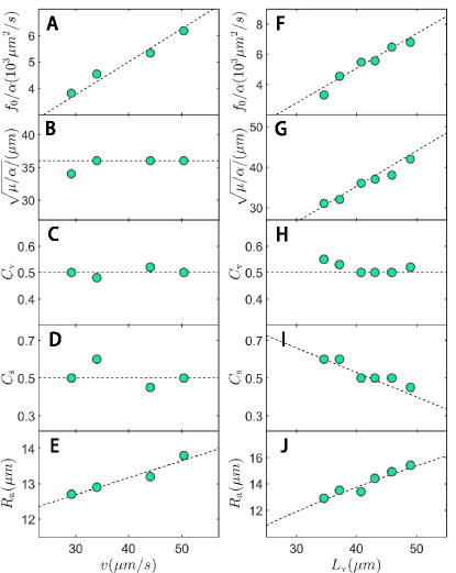
Figure 7: Variation of optimal model parameters with mean flow speed $v$ (A-E) and velocity correlation length $L_{\rm v}$. Data points in (A-E) have $L_{\rm v}\simeq 40\mu m$ and data points in (F-J) have $v\simeq 42\mu m/s$. The numerical values of all these parameters are listed in SI Appendix, Table S1. Dashed lines in A to I are linear fits (see text); dashed line in J is a fit of $R_{\rm a}\sim\sqrt{\L_{\rm v}}$ with a $R^{2}=0.925$.

Discussion

To summarize, we presented a systematic study of collective motion and defect properties in a dense, wet active nematic system composed of filamentous bacteria, and introduced a minimal microscopic model to account for our experiments. We have shown that using both orientation and velocity measurements enables to determine a unique, optimal set of parameter values at which our Vicsek-style model for active suspensions accounts quantitatively for many if not all quantities that one can extract from experimental data. Because the collective dynamics of our bacterial active nematics is always chaotic, we have used topological defects to estimate these optimal parameter values. As a matter of fact, it is sufficient to use a small subset of the various quantities we measured to determine all optimal parameter values, after which the remaining subset is “automatically” matched too. The existence of a unique optimum at which matching is nearly perfect constitutes, in retrospect, evidence of the quality of our model.

Thanks to quantitative match at a remarkable level of detail, the interplay between experiments and model provides new information and a deeper understanding of our system. This is in particular the case for the dynamics and structure of topological defects. Fig. 5C demonstrates that $+\frac{1}{2}$ defects move approximately twice as fast as the background flow. This acceleration can be explained by the local flow field (Fig. 4C), which shows two vortices above and below the strong jet advecting the defects. The shape of defects is essentially governed by the vorticity coupling constant $C_{\rm v}$ (the orientation field around $+\frac{1}{2}$ defects changes from from arrow-like to mushroom-like shape when increasing $C_{\rm v}$ (61, 73)). This cannot be seen in our experiments, in which $C_{\rm v}$ is essentially constant (Fig. 7C,H) but is shown by simulations of our quantitatively faithful model (SI Appendix, Fig. S5). Thus, the vortices can destabilize orientational order ahead of the core, causing the defect to move faster than the background flow. The accelerating effect weakens when particles are less sensitive to flow vorticity or when nematic interaction becomes stronger, as shown in simulation (SI Appendix, Fig. S4C) and experiments (Fig. 5CD).

The averaged orientation and velocity fields around $-\frac{1}{2}$ defects (Fig. 4B,D) show an approximate 3-fold rotational symmetry, which is consistent with the conventional, equilibrium picture: this symmetry implies that active and elastic stresses are balanced around the defect core, and that $-\frac{1}{2}$ defects are passive particles advected by the background flow. However, our experiments and simulations indicate that $-\frac{1}{2}$ defects possess a small but significant velocity in the fluid frame $\Delta{\bf v}^{-}$ (Fig. 3E,I,G,K,5D). Moreover, instantaneous fields around $-\frac{1}{2}$ defects often deviate significantly from 3-fold symmetry, see SI Appendix, Fig. S9. Such deviations break stress balance around the core and give $-\frac{1}{2}$ defects their velocity over the background flow. Our data (SI Appendix, Fig. S9 and S10) indeed show that the degree of deviation from 3-fold symmetry correlates with this velocity.

Our work also explains the multiple effects of cell length (under the influence of Cephalexin). Cell length directly, and not surprisingly, governs all lengthscales in our system, and does so nearly identically (Figs. 2E, 5AB, 7F-J). More surprising is the observation that the relative speed of defects decreases with cell length (Fig. 5CD) and that the strain coupling constant $C_{\rm s}$ decreases for long cells (Fig. 7I).

These findings are just a subset of all those illustrating how, thanks to the quantitative modeling, one can not only determine key effective parameters (such as the strength of flagella or the effective viscosity of our suspension) but also “read” important physical mechanisms from observing how model parameters change in experiments or are changed in simulations.

Our data-driven quantitative matching was made possible thanks to the relative simplicity of our Vicsek-style model: even though it deals with wet active suspensions, it possesses a relatively small number of parameters, and is numerically efficient. Treating near-field interactions only effectively, it is also versatile, and we believe the same approach can be applied to other active suspensions and extended to include other effects, such as external field and polar order.

The simplicity of our model should also allow to derive continuous, hydrodynamic equations. Works on hydrodynamic theories of wet active nematics abound, but they typically lack a direct connection to microscopic mechanisms. Thus deriving a faithful hydrodynamic theory from our quantitatively-valid model is a very promising step. That would in particular allow to estimate how far our active nematics deviates from elastic theory predictions, something hinted by the structure of defects (Fig. 4EF). This is the topic of ongoing work at the end of which, we hope, we will be able to build a fully quantitative link between experiments and hydrodynamic theory.

Bacteria strain and Colony Growth

We use wild type S. marcescens strain ATCC 274 labeled with green fluorescent protein p15A-eGFP. Bacteria colonies are grown on soft ($0.5\%$) Difco agar plate containing $2.5\%$ Luria Broth (Sigma). We mix Cephalexin with molten agar at $70^{\circ}C$. We then pour 40 milliliters of molten agar into a 15-cm-diameter Petri dish, which is then dried with a lid on for 16 hours ($25^{\circ}C$ and $50\%$ humidity). About $10\text{ }\mu L$ of overnight bacteria culture is then inoculated on the agar. The inoculated plates are dried for another $15\text{ min}$ without a lid, then stored in an incubator at $30^{\circ}C$ and $90\%$ humidity.

Imaging procedure

After a growth time of $8-9$ hours, collective motion is observed for as long as 2 hours near the expanding edge of a colony, in an active region about $1\text{ mm}$ wide. The colony expansion speed is approximately $2\mu m/s$, i.e. much smaller than the measured bacteria flow speed. Thus its influence on bacteria velocity measurement can be neglected. We capture bacteria motion in the central part ( $277\times 277\mu m^{2}$) of this active region through a $40\times$objective (Nikon S plan Fluor). S. marcescens colonies quickly change from mono-layer to 3 layer within $100\mu m$ from the swarming edge, thus the thickness of swarming cells are constant in the observation region. A Nikon MBE45510 filter cube (excitation $470/40nm$, emission $525/50nm$) is used for fluorescent imaging. Images are acquired by a high-speed camera (Basler acA2040-180km) at $100\text{ frame}/s$ for $30s$, during which bacteria motility remains unchanged. Bacteria form an immobile film in the central part of the colony. We take videos far enough from this immobile region .

X.-q.S., H.C. and H.P.Z. acknowledge financial support of National Natural Science Foundation of China ( Grants No. 11422427, 11774222 to H.P.Z., Grant No. 11635002 to X.-q.S. and H.C., Grants No. 11474210 and No. 11674236 to X.-q.S.). H.P.Z. thanks Program for Professor of Special Appointment at Shanghai Institutions of Higher Learning (No. GZ2016004). H.C. thanks the French ANR project “Baccterns”. H.P.Z. thanks Julia Yeomans for useful discussions at the initial stage of this work.

References

- (1) Ramaswamy S (2010) The mechanics and statistics of active matter. Annual Review of Condensed Matter Physics 1:323–345.
- (2) Vicsek T, Zafeiris A (2012) Collective motion. Phys. Rep. 517(3-4):71–140.
- (3) Marchetti MC, et al. (2013) Hydrodynamics of soft active matter. Rev. Mod. Phys. 85(3):1143–1189.
- (4) Bechinger C, Di Leonardo R, Löwen H, Reichhardt C, Volpe, Giorgio and G (2016) Active particles in complex and crowded environments. Rev. Mod. Phys. 88(4):045006.
- (5) Elgeti J, Winkler RG, Gompper G (2015) Physics of microswimmers-single particle motion and collective behavior: a review. Rep. Prog. Phys. 78(5):056601 (50 pp.)–056601.
- (6) Needleman D, Dogic Z (2017) Active matter at the interface between materials science and cell biology. Nature Reviews Materials 2(9):17048.
- (7) Cavagna A, et al. (2010) Scale-free correlations in starling flocks. Proc. Natl. Acad. Sci. U. S. A. 107(26):11865–11870.
- (8) Cavagna A, Giardina I (2014) Bird flocks as condensed matter. Annual Review of Condensed Matter Physics, Vol 5 5:183–207.
- (9) Buhl J, et al. (2006) From disorder to order in marching locusts. Science (80- ) 312(5778):1402–1406.
- (10) Berdahl A, Torney CJ, Ioannou CC, Faria JJ, Couzin ID (2013) Emergent sensing of complex environments by mobile animal groups. Science 339(6119):574–576.
- (11) Ni R, Puckett JG, Dufresne ER, Ouellette NT (2015) Intrinsic fluctuations and driven response of insect swarms. Phys. Rev. Lett. 115(11):118104.
- (12) Dombrowski C, Cisneros L, Chatkaew S, Goldstein RE, Kessler JO (2004) Self-concentration and large-scale coherence in bacterial dynamics. Phys. Rev. Lett. 93(9):098103.
- (13) Sokolov A, Aranson IS, Kessler JO, Goldstein RE (2007) Concentration dependence of the collective dynamics of swimming bacteria. Phys. Rev. Lett. 98(15):158102.
- (14) Zhang HP, Be’er A, Florin EL, Swinney HL (2010) Collective motion and density fluctuations in bacterial colonies. Proc. Natl. Acad. Sci. U. S. A. 107(31):13626–13630.
- (15) Nishiguchi D, Nagai KH, Chaté H, Sano M (2017) Long-range nematic order and anomalous fluctuations in suspensions of swimming filamentous bacteria. Phys. Rev. E 95(2):020601.
- (16) Chen C, Liu S, Shi Xq, Chate H, Wu Y (2017) Weak synchronization and large-scale collective oscillation in dense bacterial suspensions. Nature 542(7640):210–214.
- (17) Bi D, Yang X, Marchetti MC, Manning ML (2016) Motility-driven glass and jamming transitions in biological tissues. Phys. Rev. X 6(2):021011.
- (18) Yang X, et al. (2017) Correlating cell shape and cellular stress in motile confluent tissues. Proc. Natl. Acad. Sci. U.S.A. 114(48):12663–12668.
- (19) Schaller V, Weber C, Semmrich C, Frey E, Bausch AR (2010) Polar patterns of driven filaments. Nature 467(7311):73–77.
- (20) Sumino Y, et al. (2012) Large-scale vortex lattice emerging from collectively moving microtubules. Nature 483(7390):448–452.
- (21) Sanchez T, Chen DTN, DeCamp SJ, Heymann M, Dogic Z (2012) Spontaneous motion in hierarchically assembled active matter. Nature 491(7424):431–+.
- (22) Keber FC, et al. (2014) Topology and dynamics of active nematic vesicles. Science 345(6201):1135–1139.
- (23) Guillamat P, Ignes-Mullol J, Sagues F (2016) Control of active liquid crystals with a magnetic field. Proc. Natl. Acad. Sci. U.S.A. 113(20):5498–5502.
- (24) Wu KT, et al. (2017) Active matter transition from turbulent to coherent flows in confined three-dimensional active fluids. Science 355(6331):1284–+.
- (25) Suzuki K, Miyazaki M, Takagi J, Itabashi T, Ishiwata S (2017) Spatial confinement of active microtubule networks induces large-scale rotational cytoplasmic flow. Proc. Natl. Acad. Sci. U.S.A. 114(11):2922–2927.
- (26) Ellis PW, et al. (2017) Curvature-induced defect unbinding and dynamics in active nematic toroids. Nature Physics 14(1):85–90.
- (27) Palacci J, Sacanna S, Steinberg AP, Pine DJ, Chaikin PM (2013) Living crystals of light-activated colloidal surfers. Science 339(6122):936–940.
- (28) Yan J, et al. (2016) Reconfiguring active particles by electrostatic imbalance. Nature Materials 15:1095.
- (29) Bricard A, Caussin JB, Desreumaux N, Dauchot O, Bartolo D (2013) Emergence of macroscopic directed motion in populations of motile colloids. Nature 503(7474):95–98.
- (30) Theurkauff I, Cottin-Bizonne C, Palacci J, Ybert C, Bocquet L (2012) Dynamic clustering in active colloidal suspensions with chemical signaling. Phys. Rev. Lett. 108(26):268303.
- (31) Jiang HR, Yoshinaga N, Sano M (2010) Active motion of a janus particle by self-thermophoresis in a defocused laser beam. Phys. Rev. Lett. 105(26):268302.
- (32) Buttinoni I, et al. (2013) Dynamical clustering and phase separation in suspensions of self-propelled colloidal particles. Phys. Rev. Lett. 110(23):238301.
- (33) Deseigne J, Dauchot O, Chate H (2010) Collective motion of vibrated polar disks. Phys. Rev. Lett. 105(9):098001.
- (34) Kumar N, Soni H, Ramaswamy S, Sood AK (2014) Flocking at a distance in active granular matter. Nat. Commun. 5:4688–4688.
- (35) Weber CA, et al. (2013) Long-range ordering of vibrated polar disks. Phys. Rev. Lett. 110(20):208001.
- (36) Narayan V, Ramaswamy S, Menon N (2007) Long-lived giant number fluctuations in a swarming granular nematic. Science (80- ) 317(5834):105–108.
- (37) Lushi E, Wioland H, Goldstein RE (2014) Fluid flows created by swimming bacteria drive self-organization in confined suspensions. Proc. Natl. Acad. Sci. U.S.A. 111(27):9733–9738.
- (38) Wioland H, Woodhouse FG, Dunkel J, Goldstein RE (2016) Ferromagnetic and antiferromagnetic order in bacterial vortex lattices. Nat. Phys. 12(4):341–U177.
- (39) Duclos G, Erlenkämper C, Joanny JF, Silberzan P (2016) Topological defects in confined populations of spindle-shaped cells. Nature Physics 13(1):58–62.
- (40) Saw TB, et al. (2017) Topological defects in epithelia govern cell death and extrusion. Nature 544(7649):212–+.
- (41) Kawaguchi K, Kageyama R, Sano M (2017) Topological defects control collective dynamics in neural progenitor cell cultures. Nature 545(7654):327–+.
- (42) Creppy A, Praud O, Druart X, Kohnke PL, Plouraboue F (2015) Turbulence of swarming sperm. Physical Review E 92(3):2722–2722.
- (43) DeCamp SJ, Redner GS, Baskaran A, Hagan MF, Dogic Z (2015) Orientational order of motile defects in active nematics. Nat. Mater. 14(11):1110–1115.
- (44) Shi Xq, Ma Yq (2013) Topological structure dynamics revealing collective evolution in active nematics. Nat. Commun. 4:3013.
- (45) Gao T, Blackwell R, Glaser MA, Betterton MD, Shelley MJ (2015) Multiscale polar theory of microtubule and motor-protein assemblies. Phys. Rev. Lett. 114(4):048101.
- (46) Ramaswamy S, Simha RA, Toner J (2003) Active nematics on a substrate: Giant number fluctuations and long-time tails. Europhys. Lett. 62(2):196–202.
- (47) Baskaran A, Marchetti MC (2008) Enhanced diffusion and ordering of self-propelled rods. Phys. Rev. Lett. 101(26):268101.
- (48) Pismen LM (2013) Dynamics of defects in an active nematic layer. Phys. Rev. E 88(5):050502.
- (49) Ngo S, et al. (2014) Large-scale chaos and fluctuations in active nematics. Phys. Rev. Lett. 113(3):038302.
- (50) Giomi L, Bowick MJ, Ma X, Marchetti MC (2013) Defect annihilation and proliferation in active nematics. Phys. Rev. Lett. 110(22):228101.
- (51) Thampi SP, Golestanian R, Yeomans JM (2013) Velocity correlations in an active nematic. Phys. Rev. Lett. 111(11):118101.
- (52) Blow ML, Thampi SP, Yeomans JM (2014) Biphasic, lyotropic, active nematics. Phys. Rev. Lett. 113(25):248303.
- (53) Giomi L (2015) Geometry and topology of turbulence in active nematics. Phys. Rev. X 5(3):031003.
- (54) Zhou S, Sokolov A, Lavrentovich OD, Aranson IS (2014) Living liquid crystals. Proc. Natl. Acad. Sci. U.S.A. 111(4):1265–1270.
- (55) Genkin MM, Sokolov A, Lavrentovich OD, S. (2017) Topological defects in a living nematic ensnare swimming bacteria. Phys. Rev. X 7(1):011029.
- (56) Doostmohammadi A, Thampi SP, Yeomans JM (2016) Defect-mediated morphologies in growing cell colonies. Phys. Rev. Lett. 117(4):048102.
- (57) Doostmohammadi A, et al. (2015) Celebrating soft matter’s 10th anniversary: Cell division: a source of active stress in cellular monolayers. Soft Matter 11(37):7328–7336.
- (58) Zhang HP, Be’er A, Smith RS, Florin EL, Swinney HL (2009) Swarming dynamics in bacterial colonies. EPL 87:48011.
- (59) Sokolov A, Aranson IS (2012) Physical properties of collective motion in suspensions of bacteria. Phys. Rev. Lett. 109(24):248109.
- (60) Giomi L, Bowick MJ, Mishra P, Sknepnek R, Cristina Marchetti M (2014) Defect dynamics in active nematics. Philos Transact A Math Phys Eng Sci 372(2029):20130365.
- (61) Zhang R, Kumar N, Ross JL, Gardel ML, de Pablo JJ (2017) Interplay of structure, elasticity, and dynamics in actin-based nematic materials. Proc. Natl. Acad. Sci. U.S.A. 115(2):E124–E133.
- (62) Hemingway EJ, Mishra P, Marchetti MC, Fielding SM (2016) Correlation lengths in hydrodynamic models of active nematics. Soft Matter 12(38):7943–7952.
- (63) Guillamat P, Ignes-Mullol J, Sagues F (2017) Taming active turbulence with patterned soft interfaces. Nature Communications 8:564.
- (64) Doostmohammadi A, Adamer MF, Thampi SP, Yeomans JM (2016) Stabilization of active matter by flow-vortex lattices and defect ordering. Nat. Commun. 7:10557.
- (65) Doostmohammadi A, Ignés-Mullol J, Yeomans JM, Sagués F (2018) Active nematics. Nature Communications 9(1).
- (66) Thampi SP, Golestanian R, Yeomans JM (2014) Active nematic materials with substrate friction. Physical Review E 90(6).
- (67) Putzig E, Redner GS, Baskaran A, Baskaran A (2016) Instabilities, defects, and defect ordering in an overdamped active nematic. Soft Matter 12(17):3854–3859.
- (68) Srivastava P, Mishra P, Marchetti MC (2016) Negative stiffness and modulated states in active nematics. Soft Matter 12(39):8214–8225.
- (69) Guillamat P, Ignes-Mullol J, Shankar S, Marchetti MC, Sagues F (2016) Probing the shear viscosity of an active nematic film. Physical Review E 94(6):060602.
- (70) Jeffery GB (1922) The motion of ellipsoidal particles immersed in a viscous fluid. Proceedings of the Royal Society A: Mathematical, Physical and Engineering Sciences 102(715):161–179.
- (71) Vicsek T, Czirok A, Benjacob E, Cohen I, Shochet O (1995) Novel type of phase-transition in a system of self-driven particles. Phys. Rev. Lett. 75(6):1226–1229.
- (72) Chate H, Ginelli F, Montagne R (2006) Simple model for active nematics: Quasi-long-range order and giant fluctuations. Phys. Rev. Lett. 96(18):180602.
- (73) Kumar N, Zhang R, de Pablo JJ, Gardel ML (2018) Tunable structure and dynamics of active liquid crystals. Science Advances 4(10):eaat7779.