Magnonic Goos-Hänchen effect induced by one dimensional solitons

Abstract

The magnon spectral problem is solved in terms of the spectrum of a diagonalizable operator for a generic class of magnetic states that includes several types of domain walls and the chiral solitons of monoaxial helimagnets. Focusing on the isolated solitons of monoaxial helimagnets, it is shown that the spin waves scattered (reflected and transmitted) by the soliton suffer a lateral displacement analogous to the Goos-Hänchen effect of optics. The displacement is a fraction of the wavelength, but can be greatly enhanced by using an array of well separated solitons. Contrarily to the Goos-Hänchen effect recently studied in some magnetic systems, which takes place at interfaces between different magnetic systems, the effect predicted here takes place at the soliton position, what it is interesting from the point of view of applications since solitons can be created at different places and moved across the material. This kind of Goos-Hänchen effect is not particular of monoaxial helimagnets, but it is generic of a class of magnetic states, including domain walls in systems with interfacial Dzyaloshinskii-Moriya interaction.

Magnonics is a subject of much interest in recent years since it is a promising field that could transform the design of devices for information technology Chumak et al. (2015). Replacing electric currents by spin waves as information carriers in electronic devices would imply a large reduction of heat production and energy consumption due to the absence of Joule heating. Conceptual designs of devices based on spin waves have already been proposed Chumak et al. (2014); Schneider et al. (2008). One of the main challenges with spin waves is its control and manipulation. This control can be achieved in part by using the magnetic modulations of nanometric scale that are (meta)stable in some materials: domain walls, skyrmions, or chiral solitons. These solitonic states appear easily in chiral magnets, which are characterized by the presence of an important Dzyaloshinskii-Moriya interaction (DMI). Domain walls and their magnonics, with and without DMI, are being extensively studied Winter (1961); Thiele (1973); Hertel et al. (2004); Le Maho et al. (2009); Garcia-Sanchez et al. (2016); Kim et al. (2016); Borys et al. (2016); Whitehead et al. (2017); Zingsem et al. (2019). Comparatively, monoaxial helimagnets, in which the DMI acts only along one axis, called the DMI axis, have received much less attention Togawa et al. (2012); Laliena et al. (2016a, b); Shinozaki et al. (2016); Tsuruta et al. (2016); Kishine et al. (2016); Laliena et al. (2017); Goncalves et al. (2017); Laliena et al. (2018); Masaki et al. (2018); Kishine and Ovchinnikov (2020); Laliena et al. (2020).

Generically, the magnonics of the non-collinear states faces some mathematical difficulties related to the nature of the magnon wave equation. The problem is not merely technical, but it raises the question of whether a spectral representation for the spin waves exists in general, that is, whether a general solution of the linearized Landau-Lisftchitz-Gilbert (LLG) equation can be expressed as a combination of well defined spin wave modes.

In this work we develop a generic method that provides rigorously a complete solution of the spectral magnon problem in terms of the spectrum of a diagonalizable operator, for especial cases including the domain walls of many systems and the isolated soliton (IS) and the chiral soliton lattice (CSL) of monoaxial helimagnets. As a by-product, by applying this formalism, we predict the existence of a Goos-Hänchen effect in the scattering of magnons by certain localized one-dimensional magnetic modulated structures, such as solitons. Before presenting this method we analyze a general problem of magnonics, proving that the spectral representation of spin waves does exist in general.

Consider a generic magnetic system described by a magnetization vector field $\vec{M}=M_{0}\hat{n}$, with constant modulus, $M_{0}$, and direction given by the unit vector $\hat{n}$. Its energy is given by an energy functional $E[\hat{n}]$. The stationary states are those at which the variational derivative of $E[\hat{n}]$ vanishes. The (meta)stable states are the local minima of $E[\hat{n}]$, a subset of the stationary states. Let $\hat{n}_{0}$ be one stationary point of the energy. Small fluctuations around $\hat{n}_{0}$ can be written in terms of two real fields, $\xi_{1}$ and $\xi_{2}$, writing $\hat{n}=(1-\xi^{2})^{1/2}\hat{n}_{0}+\xi_{1}\hat{e}_{1}+\xi_{2}\hat{e}_{2}$, where $\{\hat{e}_{1},\hat{e}_{2},\hat{n}_{0}\}$ form an orthonormal triad. These two fields are grouped into a two component field, a “spinor” $\tilde{\xi}$, represented by the column matrix $\tilde{\xi}=[\xi_{1},\xi_{2}]^{\mathrm{T}}$. “Spinors” are denoted in this work by tilded symbols . We use the notation $(f,g)=\int d^{3}r\,f^{*}(\vec{r})\,g(\vec{r})$ for the scalar product of two functions and $\langle\tilde{\xi},\tilde{\eta}\rangle=(\xi_{1},\eta_{1})+(\xi_{2},\eta_{2})$ for the scalar product of two “spinors”.

Let us expand $E[\hat{n}]$ in powers of $\xi_{i}$ to quadratic order: $E=E_{0}+2A(1/2)\langle\tilde{\xi},K\tilde{\xi}\rangle+O(\xi^{3})$. The linear term vanishes since $\hat{n}_{0}$ is a stationary state. The constant $A$ has dimensions of energy per unit length and $K$ is a $2\times 2$ hermitian operator given

$$K=\begin{pmatrix}K_{11}&K_{12}\\ K_{12}^{\dagger}&K_{22}\end{pmatrix},$$ (1)

where $K_{11}$ and $K_{22}$ are hermitian. The $K_{ij}$ are integro-differential real operators. If $\hat{n}_{0}$ is (meta)stable, $K$ is positive (semi)definite. This requires that both $K_{11}$ and $K_{22}$ be positive (semi)definite, and imposes constraints on $K_{12}$ that we do not analyze here.

The oscillations of the magnetization about the (meta)stable state obey the LLG equation, $\partial_{t}\hat{n}=\gamma\vec{B}_{\mathrm{eff}}\times\hat{n}+\alpha\hat{n}\times\partial_{t}\hat{n}$, where $\gamma$ is the gyromagnetic constant, $\vec{B}_{\mathrm{eff}}=-\delta E/\delta\hat{n}$ is the effective field, and $\alpha$ the Gilbert damping parameter. We ignore the damping and set $\alpha=0$ in the remaining of the paper. Let us pick up some characteristic parameter of the system with units of inverse length, $q_{0}$, and introduce the constant $\omega_{0}=\gamma 2Aq_{0}^{2}/M_{0}$, with dimensions of inverse time. Considering small oscillations, we expand the LLG equation in powers of $\xi$ around $\hat{n}_{0}$. The zero-th order term vanishes since $\hat{n}_{0}$ is a stationary point. To linear order we obtain $\partial_{t}\tilde{\xi}=\Omega\tilde{\xi}$, where $\Omega=(\omega_{0}/q_{0}^{2})JK$, with

$$J=\begin{pmatrix}0&-I\\ I&0\end{pmatrix}.$$ (2)

In the above expression $I$ is the identity operator.

$\Omega$ is not anti-hermitian (not even normal), what raises the issues mentioned before about the spectral properties of the spin waves, like the existence of a complete set of well defined modes with definite frequency. We provide here a general formal answer. The spectral equation is $\Omega\tilde{\xi}=\nu\tilde{\xi}$, with $\nu$ a complex eigenvalue. For a (meta)stable state the square root of $K$ is a well defined hermitian positive (semi)definite operator. Multiplying both sides of the spectral equation by $K^{1/2}\Omega$ we obtain

$$(\omega_{0}^{2}/q_{0}^{4})\big{(}K^{1/2}JKJK^{1/2}\big{)}\,K^{1/2}\,\tilde{\xi}=\nu^{2}\,K^{1/2}\tilde{\xi}.$$ (3)

Hence, the spectral properties of $\Omega$ are derived from the spectral properties of $K^{1/2}JKJK^{1/2}$, which is hermitian, and therefore has a complete set of orthogonal eigenstates, denoted by $\{\tilde{\eta}_{i}\}$. Then $\{\tilde{\xi}_{i}=K^{-1/2}\tilde{\eta}_{i}\}$ is a complete set of eigenstates of $\Omega$, which satisfy the normalization condition $\langle\tilde{\xi}_{i},K\tilde{\xi}_{j}\rangle=\delta_{ij}$. It is easily checked that $K^{1/2}JKJK^{1/2}$ is negative (semi)definite, so that $\nu^{2}\leq 0$, and $\nu=\mathrm{i}\omega$, with $\omega$ real. Thus, for a (meta)stable state, the spectrum of $\Omega$ lies on the imaginary axis and its eigenstates form a complete set .

The spectral problem for $\Omega$ is easy if the four operators $K_{ij}$ commute, as in ferromagnetic (FM), helical, and conical states Laliena and Campo (2017), and in some domain walls Winter (1961). In those cases the problem is reduced to find the spectrum of one hermitian operator ($K_{11}$ for instance) and the diagonalization of a $2\times 2$ matrix.

In what follows, we address problems in which the $K_{ij}$ do not commute, focusing on the cases were $K_{12}=0$, for which we give a complete solution. Examples include the IS and the CSL of monoaxial helimagnets, and the domain walls of some systems with DMI Borys et al. (2016). In this last instance the authors addressed the problem via perturbation theory, splitting $\Omega_{2}$ as the sum of an operator that commutes with $\Omega_{1}$ plus a perturbation. This may be a reasonably approach, especially if the unperturbed operator can be treated analytically, provided it can be guaranteed that the perturbation does not originate new bound states.

Let us define $\Omega_{1}=(\omega_{0}/q_{0}^{2})K_{11}$ and $\Omega_{2}=(\omega_{0}/q_{0}^{2})K_{22}$. As shown above, the eigenvalues of $\Omega$ for a (meta)stable state are purely imaginary, $\mathrm{i}\omega$, with $\omega$ real. In components, the spectral equation for $\Omega$ gives $\Omega_{2}\,\xi_{2}=-\mathrm{i}\omega\,\xi_{1}$ and $\Omega_{1}\,\xi_{1}=\mathrm{i}\omega\,\xi_{2}$. Substituting the values of $\xi_{1}$ and $\xi_{2}$ given explicitly by one of these equations into the other, we obtain $\Omega_{2}\Omega_{1}\xi_{1}=\omega^{2}\xi_{1}$ and $\Omega_{1}\Omega_{2}\xi_{2}=\omega^{2}\xi_{2}$. These two equations are compatible since $\Omega_{2}\Omega_{1}$ and $\Omega_{1}\Omega_{2}$ have the same spectrum: if $\xi_{1}$ is an eigenfunction of $\Omega_{2}\Omega_{1}$ then $\Omega_{1}\xi_{1}$ is an eigenfunction of $\Omega_{1}\Omega_{2}$ with the same eigenvalue; the same is true changing 1 by 2. The case $\omega=0$ is special: if $\xi_{1}$ is an eigenfunction of $\Omega_{2}\Omega_{1}$ with zero eigenvalue, we have an eigenstate of $\Omega$ just taking $\xi_{2}=0$. Again, the statement is valid changing 1 by 2.

The $K$ operator of a (metas)stable state may be gapless or even have zero modes. When $K_{12}=0$ the zero modes or the gapless modes are generically associated to one operator, say $K_{11}$, and $K_{22}$ has a gap. Hence $\Omega_{2}$ is a hermitian positive definite invertible operator, and so it is its square root. Therefore, although $\Omega_{2}\Omega_{1}$ is not hermitian (not even normal), equation $\Omega_{2}\Omega_{1}\xi_{1}=\omega^{2}\xi_{1}$ can be written in terms of the hermitian positive semidefinite operator $\Lambda=\Omega_{2}^{1/2}\,\Omega_{1}\,\Omega_{2}^{1/2}$ as $\Lambda\,\big{(}\Omega_{2}^{-1/2}\xi_{1}\big{)}=\omega^{2}\,\big{(}\Omega_{2}^{-1/2}\xi_{1}\big{)}$. Therefore, the spectral problem for $\Omega$ is completely solved in terms of the spectral problem $\Lambda\upsilon=\omega^{2}\upsilon$, just setting $\xi_{1}=\Omega_{2}^{1/2}\upsilon$ and $\xi_{2}=\Omega_{2}^{-1/2}\upsilon$, where we used the equation $\Omega_{2}\,\xi_{2}=-\mathrm{i}\omega\,\xi_{1}$. If $\{\upsilon_{i}\}$ is a complete set of orthonormal eigenfunctions of $\Lambda$, then $\{\psi_{i}=\omega_{0}^{-1/2}\,\Omega_{2}^{1/2}\,\upsilon_{i}$} is a complete set of eigenfunctions of $\Omega_{2}\,\Omega_{1}$ that satisfy the condition

$$(\psi_{i},\,\omega_{0}\,\Omega_{2}^{-1}\,\psi_{j})=N_{i}\,\delta_{ij},$$ (4)

where $N_{i}$ provides a proper normalization condition .

We find it convenient to express the eigenstates of $\Omega$ in terms of the eigenfunctions of $\Omega_{2}\Omega_{1}$, $\psi_{i}$. Since $\Omega$ is real, its spectrum comes in complex conjugate pairs. Hence, each $\psi_{i}$ gives rise to two eigenstates of $\Omega$, with eigenvalues $\mathrm{i}\sigma\omega_{i}$, with $\omega_{i}\geq 0$ and $\sigma=\pm 1$, given by

$$\tilde{\xi}^{(i\,\sigma)}=\frac{1}{(1+\omega_{i}^{2}/\omega_{0}^{2})^{1/2}}\begin{pmatrix}\psi_{i}\\ -\mathrm{i}\sigma\omega_{i}\Omega_{2}^{-1}\psi_{i}\end{pmatrix},$$ (5)

which satisfy the normalization condition

$$\langle\tilde{\xi}^{(i\,\sigma)},G\tilde{\xi}^{(j\,\sigma^{\prime})}\rangle=\frac{\omega_{0}^{2}+\sigma\sigma^{\prime}\omega_{i}^{2}}{\omega_{0}^{2}+\omega_{i}^{2}}N_{i}\delta_{ij},$$ (6)

where

$$G=\begin{pmatrix}\omega_{0}\Omega_{2}^{-1}&0\\ 0&\omega_{0}^{-1}\Omega_{2}\end{pmatrix}.$$ (7)

The completitude of the set $\{\psi_{i}\}$ implies the completitude of the set $\{\tilde{\xi}^{(i\sigma)}\}$: for any given $\tilde{\xi}$ we have $\tilde{\xi}=\sum_{i\sigma}c_{i\sigma}\tilde{\xi}^{(i\sigma)}$, where, defining $\bar{\sigma}=-\sigma$,

$$c_{i\sigma}\!=\!\frac{\big{(}\omega_{i}^{2}+\omega_{0}^{2}\big{)}^{2}}{4N_{i}\omega_{0}^{2}\omega_{i}^{2}}\!\left[\!\big{\langle}\tilde{\xi}^{(i\sigma)},G\tilde{\xi}\big{\rangle}\!+\!\frac{\omega_{i}^{2}-\omega_{0}^{2}}{\omega_{i}^{2}+\omega_{0}^{2}}\!\big{\langle}\tilde{\xi}^{(i,\bar{\sigma})},G\tilde{\xi}\big{\rangle}\!\right]\!.$$ (8)

In summary, we have obtained the eigenstates $\tilde{\xi}^{i\sigma}$ of $\Omega$ in terms of the eigenfunctions $\psi_{i}$ of the diagonalizable operator $\Omega_{2}\Omega_{1}$, for the cases in which $K_{12}=0$, what allows to solve a number of important problems. Moreover, Eqs. (5)-(8) can be taken as a starting point to quantization, by imposing canonical commutation relations to $\xi_{1}$ and $\xi_{2}$, which are derived from the algebra of angular momentum satisfied by the quantized components of $\hat{n}$.

In the following we apply this method to the case of an IS in a monoaxial helimagnet, which is characterized by an energy functional $E[\hat{n}]=2A\int d^{3}rW$, with

$$W=\frac{1}{2}\partial_{i}\hat{n}\cdot\partial_{i}\hat{n}-q_{0}\hat{z}\cdot(\hat{n}\times\partial_{z}\hat{n})-\frac{1}{2}q_{0}^{2}\kappa(\hat{z}\cdot\hat{n})^{2}-q_{0}^{2}\vec{h}\cdot\hat{n}.$$ (9)

The successive terms of the right-hand side represent a FM exchange interaction, a uniaxial DMI along the $\hat{z}$ axis, an easy-plane ($\kappa<0$) uniaxial magnetic anisotropy (UMA) along the DMI axis, and a Zeeman interaction with an external magnetic field perpendicular to the DMI axis, with $\vec{h}=h\hat{y}$. For simplicity, we ignore the magnetostatic energy. The constant $q_{0}$ is proportional to the ratio between the DMI and FM exchange interaction strengths, and plays the role of the $q_{0}$ parameter introduced above, and $\kappa$ and $\vec{h}$ are dimensionless. The numerical results discussed below correspond to $\kappa=-5.0$ and $h=1.0$, unless other values are explicitly quoted.

The Sine-Gordon soliton is a stationary point, given by $\hat{n}_{0}=-\sin\varphi\,\hat{x}+\cos\varphi\,\hat{y}$, with $\varphi(z)=4\arctan[\exp(z/\Delta)]$, where $\Delta=1/(q_{0}\sqrt{h})$ is the soliton width. Notice that $\hat{n}_{0}$ is confined to the plane perpendicular to the DMI axis. The solitons are metastable below a certain value of $h$ that depends on the DMI and UMA strengths Laliena et al. (2020), and they condense into a CSL for $h$ below the critical field $h_{c}=\pi^{2}/16$ Dzyaloshinskii (1964).

Taking $\hat{e}_{1}=\hat{z}\times\hat{n}_{0}$ and $\hat{e}_{2}=\hat{z}$, so that $\xi_{1}$ and $\xi_{2}$ describe the in-plane and out-of-plane oscillations, respectively, the operators $\Omega_{1}$ and $\Omega_{2}$ are given by

$$\Omega_{1} = \frac{\omega_{0}}{q_{0}^{2}}\big{[}-\nabla^{2}+U_{1}+q_{0}^{2}h\big{]},$$ (10)

$$\Omega_{2} = \frac{\omega_{0}}{q_{0}^{2}}\big{[}-\nabla^{2}+U_{2}+q_{0}^{2}(h-\kappa)\big{]},$$ (11)

where $U_{1}=-(1/2)\varphi^{\prime\,2}$ and $U_{2}=-(3/2)\varphi^{\prime\,2}+2q_{0}\varphi^{\prime}$ are even functions of $z$ and decay exponentially to zero when $z\rightarrow\pm\infty$, since $\varphi^{\prime}(z)=2/[\Delta\cosh(z/\Delta)]$. These functions are independent of $\kappa$, but depend on $h$ through $\Delta$.

The operators $\Omega_{1}$ and $\Omega_{2}$ are partially diagonalized by a Fourier transform in $x$ and $y$. Since $x$ and $y$ enter the problem in a symmetric way, to simplify the notation we consider only the $x$ dependence, writing the eigenfunctions of $\Omega_{2}\Omega_{1}$ as $\psi_{k_{x}}(x,z)=\exp(\mathrm{i}k_{x}x)\phi_{k_{x}}(z)$. The general case is obtained by replacing $k_{x}^{2}$ by $k_{x}^{2}+k_{y}^{2}$ and $\exp(\mathrm{i}k_{x}x)$ by $\exp[\mathrm{i}(k_{x}x+k_{y}y)]$. After the Fourier transform, the spectral problem becomes $\Omega_{2k_{x}}\Omega_{1k_{x}}\phi_{k_{x}}=\omega^{2}\phi_{k_{x}}$, where $\omega^{2}$ is a function of $k_{x}^{2}$ and

$$\Omega_{1k_{x}}=\Omega_{10}+\omega_{0}k_{x}^{2}/q_{0}^{2},\quad\Omega_{2k_{x}}=\Omega_{20}+\omega_{0}k_{x}^{2}/q_{0}^{2},$$ (12)

with $\Omega_{10}$ and $\Omega_{20}$ obtained by replacing $\nabla^{2}$ by $\partial_{z}^{2}$ in $\Omega_{1}$ and $\Omega_{2}$. The eigenfunctions, $\phi_{k_{x}i}$, labeled by $i$, satisfy a normalization condition analogous to (4).

Non-reciprocal propagation, usually associated to chirality, is absent in the IS and in the CSL, because it require first order derivatives in the $\Omega$ operator, which is not the case. It is easy to see, by deriving the generic form of the $K$ operator associated to (9), that non-reciprocal propagation takes place in monoaxial helimagnets only in states whose magnetic moments have a non-vanishing projection onto the DMI axis.

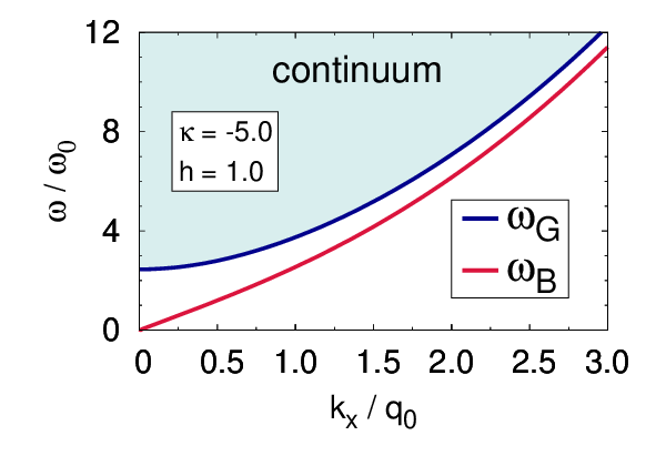
The spectral problems were solved numerically for a large discrete set of $k_{x}$, on a box $-L\leq z\leq L$ with Dirichlet boundary conditions at $z=\pm L$ Laliena and Campo (2020). Insight about the spectrum is obtained by studying the asymptotic properties of the eigenfunctions as $z\rightarrow\pm\infty$, given in the supplemental material Laliena and Campo (2020). The spectrum, depicted in Fig. 1 (right), contains a continuum of states unbounded in all directions, with frequencies above a gap given by

$$\omega_{\mathrm{G}}(k_{x})=\omega_{0}\big{[}(k_{x}^{2}/q_{0}^{2}+h)(k_{x}^{2}/q_{0}^{2}+h-\kappa)\big{]}^{1/2},$$ (13)

which is obtained by standard means from the asymptotic analysis Laliena and Campo (2020). Below the gap there is a gapless branch of states, consisting of waves bounded to the soliton position, that is, decaying exponentially as $z\rightarrow\pm\infty$, but unbounded in the other directions.

Figure 1: Left: spin wave spectrum. The red line is the dispersion relation, $\omega_{\mathrm{B}}(k_{x})$, for the bound state branch, and the blue line signals the gap. Right: Phase shifts $\delta_{0}$ (continuous lines) and $\delta_{1}$ (broken lines) vs. $k_{z}$ for $k_{x}=0$ for the indicated values of $h$.

We shall analyze the gapless branch elsewhere. Here we focus on the continuum states, that are used to describe the scattering of a magnon wave packet by the soliton, which results in the emergence of one reflected and one transmitted wave packet (the scattered waves). Although $\Omega_{2k_{x}}\Omega_{1k_{x}}$ is not hermitian, nor second order in derivatives, the concepts of scattering theory are valid since they rely only on the asymptotic properties of the wave equation Galindo and Pascual (1990). This allows us to predict one unusual feature of the scattering: the Goos-Hänchen effect.

The eigenfunctions $\Omega_{2k_{x}}\Omega_{1k_{x}}$ are either even or odd functions of $z$, due to the $z\rightarrow-z$ invariance. The continuum states are degenerate, and for each $\omega^{2}$ there is an even and an odd eigenfunction, behaving as $z\rightarrow\pm\infty$ as

$$\phi^{(e)}_{k_{x}k_{z}}(z)\sim\cos(k_{z}z\pm\delta_{0}),\;\;\phi^{(o)}_{k_{x}k_{z}}(z)\sim\sin(k_{z}z\pm\delta_{1}),$$ (14)

where the superscripts $e$ and $o$ stand for even and odd, respectively, and $\delta_{0}$ and $\delta_{1}$ are the corresponding phase shifts, which depend on $k_{x}$ and $k_{z}$. The wave number $k_{z}$ is obtained from $\omega^{2}$ using the dispersion relation Laliena and Campo (2020):

$$k_{z}=q_{0}\left[\left(\frac{\omega^{2}}{\omega_{0}^{2}}+\frac{\kappa^{2}}{4}\right)^{1/2}-\left(\frac{k_{x}^{2}}{q_{0}^{2}}+h-\frac{\kappa}{2}\right)\right].$$ (15)

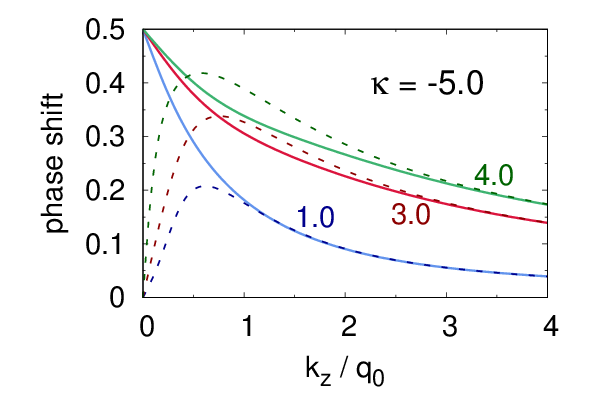
The phase shifts are obtained by combining the asymptotic behaviour of Eqs. (14) and the boundary condition at $z=L$, what gives $k_{z}L+\delta_{i}=2\pi n_{i}$, for $i=0,1$, where $n_{i}$ are integers and $\delta_{i}\in[-\pi,\pi]$. The phase shifts for $k_{x}=0$ are shown as a function of $k_{z}$ in Fig. 1 (right). In contrast with the the domain wall case Winter (1961), which is reflectionless for magnons, the reflection coefficient, $R=\sin^{2}(\delta_{0}-\delta_{1})$, does not vanish since $\delta_{0}\neq\delta_{1}$.

It is curious that, in spite that it has been demonstrated only for some classes of Schrödinger operators, and $\Omega_{2k_{x}}\Omega_{1k_{x}}$ is not a Schrödinger operator, the phase shifts agree with the thesis of Levinson theorem Galindo and Pascual (1990); Levinson (1949), which states that $[\delta_{0}(0)-\delta_{0}(\infty)]/\pi+1/2$ and $[\delta_{1}(0)-\delta_{1}(\infty)]/\pi$ are equal to the number of bound states of the respective parities. The agreement follows from $\delta_{0}=\pi/2$ and $\delta_{1}=0$ for $k_{z}=0$, $\delta_{0}=\delta_{1}=0$ for $k_{z}\rightarrow\infty$, and the existence of a single bound state (gapless branch), which is even.

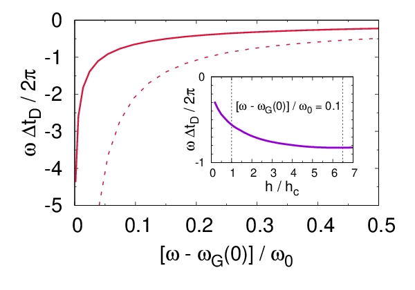
The dependence of the phase shifts on the frequency introduces a time delay in the scattered (reflected and transmitted) waves given by $\Delta t_{D}=d(\delta_{0}+\delta_{1})/d\omega$ Wigner (1955). It is indeed an advance time, since we obtain $\Delta t_{D}<0$. This is usually the case when the scattering potential is repulsive, so that we may conclude that the soliton repels the magnons. It was shown by Wigner that causality implies the bound $\Delta t_{D}\geq-(2ak+1)/kv$, where $a$ is the range of the potential, $k^{2}=k_{x}^{2}+k_{z}^{2}$, and $v=d\omega/dk$ is the group velocity Wigner (1955). In our case we may reasonably estimate the bound taking $a=\Delta$. The product $\omega\Delta t_{D}$ versus $\omega-\omega_{G}$ is shown in Fig. 2 (left) for $k_{x}=0$. The Wigner bound (broken line) is well satisfied. The delay time is appreciable for frequencies close to $\omega_{G}$ and, as the inset shows, decreases with the magnetic field strength.

The non trivial dependence of $\Omega_{2k_{x}}\Omega_{1k_{x}}$ on $k_{x}$ induces a $k_{x}$ dependence of the phase shifts, which originates a displacement of the scattered waves (reflected and transmitted) perpendicular to $\hat{z}$. That is, if the center of a wave packet of narrow cross section impinges the soliton at a point $x$, the scattered wave packets left the soliton centered at a point $x+\Delta x$, where $\Delta x=-\partial(\delta_{0}+\delta_{1})/\partial k_{x}$. This relation is derived from a stationary phase analysis of the scattered wave Artmann (1948). This very interesting effect is analogous to the well known Goos-Hänchen effect of optics Goos and Hänchen (1947), in which a light beam reflected at the interface of two different media suffers a lateral displacement given by an expression similar to the above $\Delta x$. Recently, the Goos-Hänchen effect for spin waves has been theoretically studied at interfaces that separate different magnetic media Dadoenkova et al. (2012); Gruszecki et al. (2014, 2015, 2017); Mailyan et al. (2017); Wang et al. (2019); Zhen and Deng (2020), and experimental evidence of the effect at the edge of a Permalloy film has been reported Stigloher et al. (2018). To our knowledge, the kind of Goos-Hänchen effect predicted here, induced by a magnetic modulation instead of an interface, has not been considered before.

The Goos-Hänchen shift produced by magnetic modulations (not by interfaces) is due to the non-commutativity of $\Omega_{1k_{x}}$ and $\Omega_{2k_{x}}$: if they commute, the phase shifts are independent of $k_{x}$, since then the eigenfunctions of $\Omega_{1k_{x}}\Omega_{2k_{x}}$ are the eigenfunctions of $\Omega_{1k_{x}}$ or $\Omega_{2k_{x}}$, which are independent of $k_{x}$, because $k_{x}$ enters this operators through a multiple of the identity. Examples in which $\Omega_{1k_{x}}$ and $\Omega_{2k_{x}}$ do commute are the usual domain walls Winter (1961), which therefore do not induce the Goos-Hänchen effect. The addition of an interfacial DMI, as in the model studied by Borys et al. Borys et al. (2016), spoils the commutativity of $\Omega_{1k_{x}}$ and $\Omega_{2k_{x}}$ and therefore induce a Goos-Hänchen effect in this kind of domain walls. Borys et al. did not address this question since they consider only the propagation of spin waves in one dimension. To our knowledge, the Goos-Hänchen effect has not been analyzed yet in domain walls, in spite that it has to appear in some of them (e.g. those with DMI). It can be done following the ideas presented in this work.

Figure 2: Left: time delay in units of the wave period vs. frequency $\omega-\omega_{\mathrm{G}}(0)$. The broken line is the Wigner causal bound. Inset: time delay vs. $h/h_{c}$ for $\omega-\omega_{\mathrm{G}}(0)=0.1\,\omega_{0}$. Right: Goos-Hänchen shift for several incidence angles, in degrees, for $h=h_{c}$. Inset: transmission coefficient for the same angles.

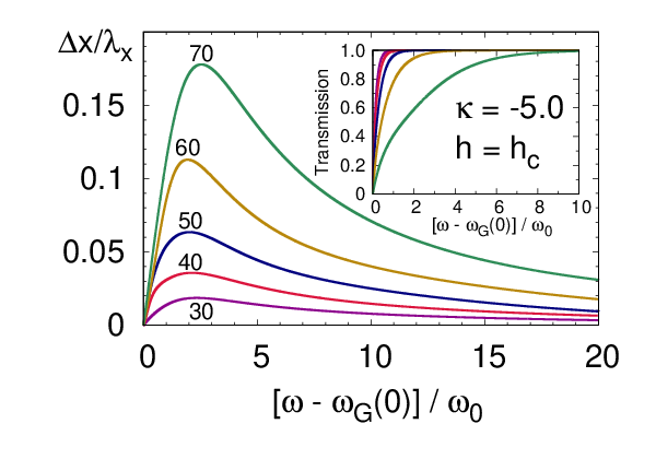
The shift $\Delta x$ that we obtain for the IS in a monoaxial helimagnet is a fraction of the wavelength in the $\hat{x}$ direction, $\lambda_{x}=2\pi/k_{x}$. This is very interesting because it opens the possibility of manipulating the spin waves at the sub-wavelength scale. Moreover, $\Delta x$ is additive as the wave is transmitted across an array of well separated solitons, and therefore the shift can be enhanced by a large factor, provided the transmission coefficient is high enough. The magnitude of the shift decreases with the magnetic field, which acts as a control parameter. Fig. 2 (right) displays $\Delta x/\lambda_{x}$ as a function of frequency (relative to $\omega_{\mathrm{G}}$) for several values of the incidence angle, for the critical field $h=h_{c}$. At this value of $h$ solitons can be easily created. The inset shows the transmission coefficient for the same angles. We see that there is a range of frequencies and incidence angles where $\Delta x/\lambda_{x}\approx 0.1$ and the transmission coefficient is very close to one, so that $\Delta x$ can be enhanced to several tens of wavelengths.

To conclude, it is worthwhile to stress that the Goos-Hänchen displacement predicted here is not particular of monoaxial helimagnets, but it is expected in any one-dimensional soliton for which $\Omega_{10}$ and $\Omega_{20}$ do not commute, for instance in domain walls with DMI Borys et al. (2016). It is also remarkable that it does not take place at the interface between two different magnetic media, but at the soliton position. For potential applications, this has the advantage that solitons can be created at different locations and moved across the material by the application of magnetic fields or polarized currents Laliena et al. (2020).