Gradient Episodic Memory with a Soft Constraint for Continual Learning

Abstract

Catastrophic forgetting in continual learning is a common destructive phenomenon in gradient-based neural networks that learn sequential tasks, and it is much different from forgetting in humans, who can learn and accumulate knowledge throughout their whole lives. Catastrophic forgetting is the fatal shortcoming of a large decrease in performance on previous tasks when the model is learning a novel task. To alleviate this problem, the model should have the capacity to learn new knowledge and preserve learned knowledge. We propose an average gradient episodic memory (A-GEM) with a soft constraint $\epsilon\in[0,1]$, which is a balance factor between learning new knowledge and preserving learned knowledge; our method is called gradient episodic memory with a soft constraint $\epsilon$ ($\epsilon$-SOFT-GEM). $\epsilon$-SOFT-GEM outperforms A-GEM and several continual learning benchmarks in a single training epoch; additionally, it has state-of-the-art average accuracy and efficiency for computation and memory, like A-GEM, and provides a better trade-off between the stability of preserving learned knowledge and the plasticity of learning new knowledge.

1 Introduction

In general, humans observe data as a sequence and seldom observe the samples twice; otherwise, they can learn and accumulate knowledge of new data throughout their whole lives. Unlike humans, artificial neural networks (ANNs), which are inspired by biological neural systems, suffer from catastrophic forgetting [1, 2, 3], whereby learned knowledge is disrupted when a new task is being learned.

Continual learning [4, 5, 6] aims to alleviate catastrophic forgetting in ANNs. The key to continual learning is that the model handles the data individually and preserves the knowledge of previous tasks without storing all the data from previous tasks. With continual learning, the model has the potential to learn novel tasks quickly if it can consolidate the previously acquired knowledge. Unfortunately, in the most common approaches, the model cannot learn new knowledge about previous tasks when acquiring new knowledge of new tasks in order to alleviate catastrophic forgetting. For example, EWC[7], PI [8], RWALK [9] and MAS [10], which use regularization to slow down learning with weights that correlate with previously acquired knowledge, resist decreasing the performance on previous tasks and cannot acquire new knowledge fast. The assumption of gradient episodic memory (GEM) [11] and average gradient episodic memory (A-GEM) [12] is that the model guarantees to avoid increasing the loss over episodic memory when the model updates the gradient, which has the same shortcoming.

Catastrophic forgetting can be alleviated if the model can acquire novel knowledge about previous tasks when learning new tasks. Building on GEM and A-GEM, we assume that the model not only maintains the loss over episodic memory, preventing it from increasing, but actually decreases the loss to acquire novel knowledge of experiences that are representative of the previous tasks. To achieve this goal, the optimizer of the model should guarantee that the angle between the gradient of samples from episodic memory and the updated gradient is less than $90^{\circ}$. Based on the idea above, we introduce a soft constraint $\epsilon\in[0,1]$, which is a balance between forgetting old tasks (loss over previous tasks that are represented by episodic memory) and learning new tasks (loss over new tasks), and propose a variant of A-GEM with a soft constraint $\epsilon$, called $\epsilon$-SOFT-GEM, which is a combination of episodic memory and optimization constraints. Additionally, we introduce an intuitive idea, average A-GEM (A-A-GEM), in which the updated gradient is the average of the gradient of samples from episodic memory and the gradient of new samples from learning task, and the angle between the gradient of the samples from episodic memory and the updated gradient must be no more than $90^{\circ}$.

We evaluate $\epsilon$-SOFT-GEM, A-A-GEM and several representative baselines on a variety of sequential learning tasks on the metrics of the stability and plasticity of the model. Our experiments demonstrate that $\epsilon$-SOFT-GEM achieves better performance than A-GEM with almost the same efficiency in terms of computation and memory; meanwhile, $\epsilon$-SOFT-GEM outperforms other common continual learning benchmarks in a single training epoch.

2 Related Work

The term catastrophic forgetting was first introduced by [2], who claimed that catastrophic forgetting is a fundamental limitation of neural networks and a downside of their high generalization ability. The cause of catastrophic forgetting is that ANNs are based on concurrent learning, where the whole population of the training samples is presented and trained as a single and complete entity; therefore, alterations to the parameters of ANNs using back-propagation lead to catastrophic forgetting when training on new samples.

Several works have described destructive consequences of catastrophic forgetting in sequential learning and provided a few primitive solutions, such as employing experience replay with all previous data or subsets of previous data [13, 14].

Other works focus on training individual models or sharing structures to alleviate catastrophic forgetting. A progressive neural network (PROGNN) [15] has been proposed to train individual models on each task, retain a pool of pretrained models and learn lateral connections from these to extract useful features for new tasks, which eliminates forgetting altogether but requires growing the network after each task and can cause the architecture complexity to increase with the number of tasks. DEN [16] can learn a compact overlapping knowledge-sharing structure among tasks. PROGNN and DEN require the number of parameters to be constantly increased and thus lead to a huge and complex model.

Many works focus on optimizing network parameters on new tasks while minimizing alterations to the consolidated weights on previous tasks. It is suggested that regularization methods, such as dropout[17], L2 regularization and activation functions [18, 19], help to reduce forgetting for previous tasks [20]. Furthermore, EWC [7] uses a Fisher information matrix-based regularization to slow down learning on network weights that correlate with previously acquired knowledge. PI [8] employs the path integrals of loss derivatives to slow down learning on weights that are important for previous tasks. MAS [10] accumulates an importance measure for each parameter of the network and penalizes the important parameters. RWALK [9] introduces a distance in the Riemannian manifold as a means of regularization. The regularization methods resist decreasing the performance on previous tasks and learn new tasks slowly.

Episodic memory can store previously seen samples and replay them; iCarl [21] replays the samples in episodic memory, while GEM [11] and A-GEM [12] use episodic memory to make future gradient update. However, choosing samples from previous tasks is challenging since it requires knowing how many samples to store and how the samples represent the tasks. The experience replay strategies proposed in [22] are reservoir sampling [23], ring buffer [11], k-means and mean of features [21].

3 Gradient Episodic Memory with a Soft Constraint

For $\epsilon$-SOFT-GEM, the learning protocol is described in [12], and the sequential learning task is divided into two ordered sequential streams $D^{CV}=\{D_{1},...,D_{T^{CV}}\}$ and $D^{EV}=\{D_{T^{CV}+1},...,D_{T}\}$, where $D_{k}=\{(\mathbf{x}_{i}^{k},t_{i}^{k},y_{i}^{k})_{i=1}^{n_{k}}\}$ is the dataset of the $k$-th task, $T^{CV}<T$. $D^{CV}$ is the stream of datasets used in cross-validation to select the hyperparameters of the model, and $D^{EV}$ is the stream of datasets used for training and evaluation.

3.1 GEM

In this section, we review GEM, which is a model for continual learning with an episodic memory $\mathcal{M}_{k}$ for each task $k$, which stores a subset of the observed examples or embedding features from task $k$. GEM defines the loss over $\mathcal{M}_{k}$ as:

$$l(f_{\theta},\mathcal{M}_{k})=\frac{1}{|\mathcal{M}_{k}|}\sum_{(\mathbf{x}_{i},k,y_{i})\in\mathcal{M}_{k}}l(f_{\theta}(\mathbf{x}_{i},k),y_{i}).$$ (1)

GEM avoids catastrophic forgetting by storing an episodic memory $\mathcal{M}_{k}$ for each task $k$; therefore, the intuitive idea is that it guarantees to avoid increasing the losses over episodic memories of tasks. Formally, for task $t$, GEM solves for the following objective:

$$\begin{array}[]{ll}\text{minimize}_{\theta}&l(f_{\theta},\mathcal{D}_{t})\\ \text{subject to}&l(f_{\theta},\mathcal{M}_{k})-l(f_{\theta}^{t-1},\mathcal{M}_{k})\leq 0,\quad\forall k<t,\end{array}$$ (2)

where $f_{\theta}^{t-1}$ is the trained network until task $t-1$. The dual optimization problem of GEM is given by:

$$\begin{array}[]{ll}\text{minimize}_{\widetilde{g}}&\frac{1}{2}||g-\widetilde{g}||_{2}^{2}\\ \text{subject to}&\langle\widetilde{g},g_{k}\rangle\geq 0,\quad\forall k<t,\end{array}$$ (3)

where $\langle g,g_{k}\rangle=\left\langle\frac{\partial l(f_{\theta}(\mathbf{x},t),y)}{\partial\theta},\frac{\partial l(f_{\theta},\mathcal{M}_{k})}{\partial\theta}\right\rangle$.

The basic idea of GEM is shown in Figure 1(a), where $g_{1}$ and $g_{2}$ are the gradients of samples from $\mathcal{M}_{1}$ and $\mathcal{M}_{2}$ respectively, $g$ is the gradient of samples from the current task, $\widetilde{g}$ is the updated gradient, and $\lambda=90^{\circ}$.

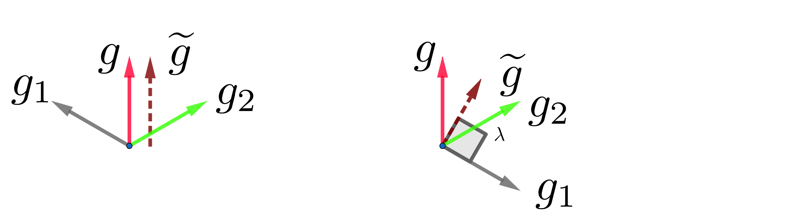
(a)

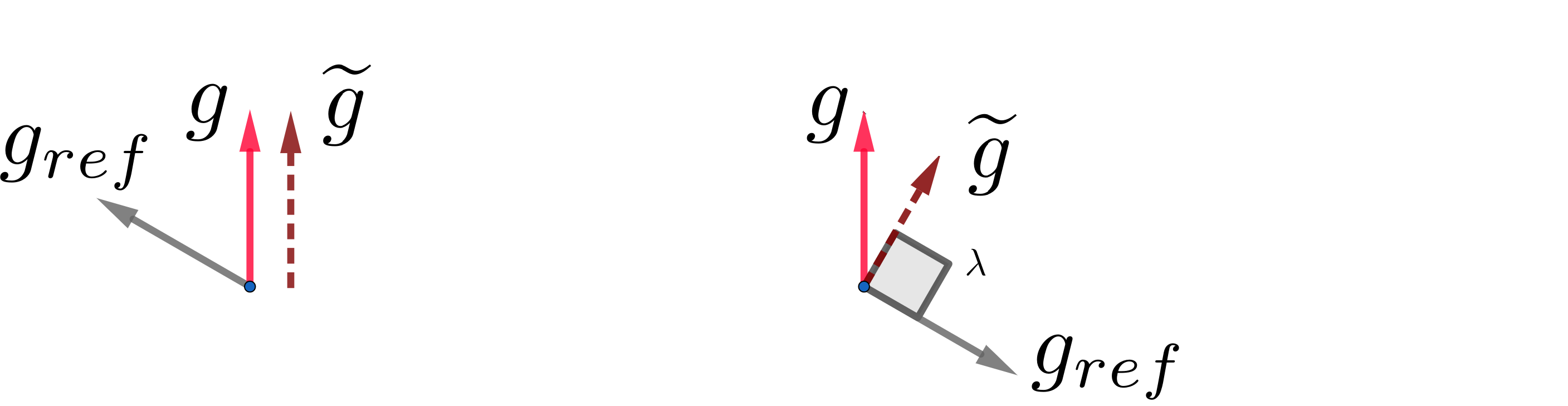
(b)

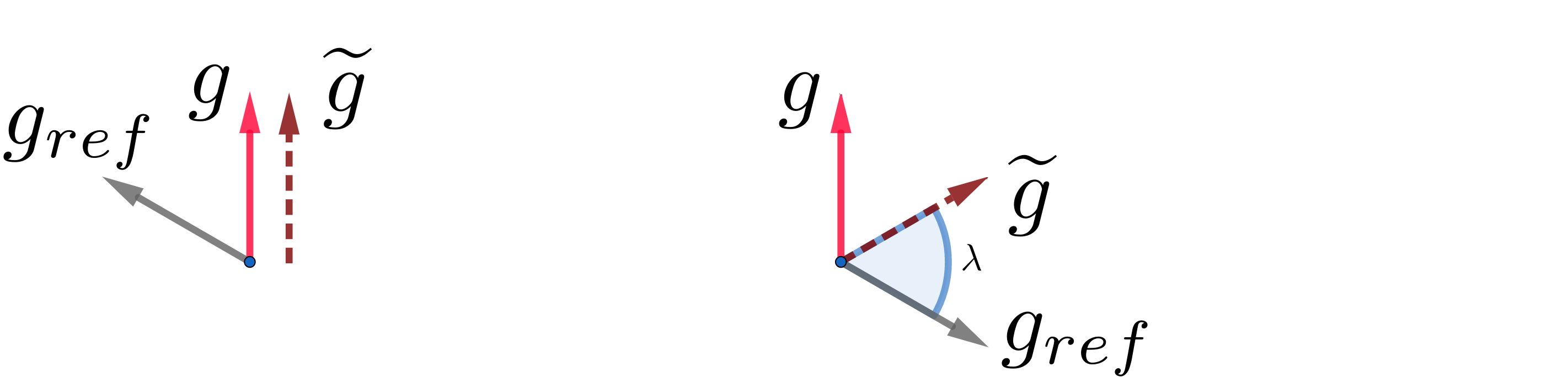
(c)

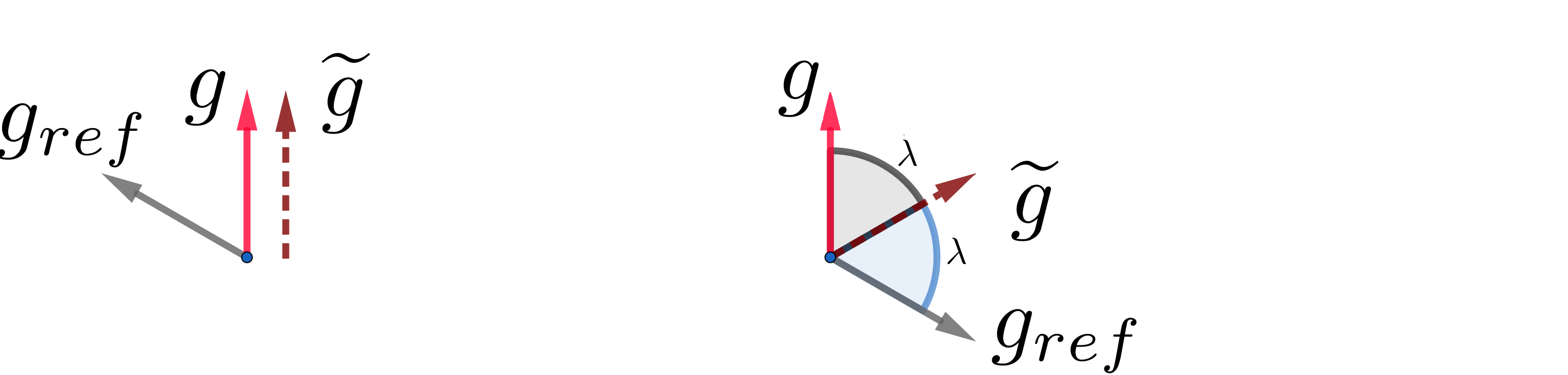
(d)

Figure 1: The basic ideas of GEM, A-GEM, $\epsilon$-SOFT-GEM and A-A-GEM.

3.2 A-GEM

GEM computes the matrix $G=-(g_{1},g_{2},...,g_{t-1})$ by using samples from episodic memory, which requires much computation. The average GEM (A-GEM) [12] aims to ensure that at every training step, the average episodic memory loss over the previous tasks does not increase. Formally, the objective of A-GEM is:

$$\begin{array}[]{ll}\text{minimize}_{\theta}&l(f_{\theta},\mathcal{D}_{t})\\ \text{subject to}&l(f_{\theta},\mathcal{M})\leq l(f_{\theta}^{t-1},\mathcal{M}),\mathcal{M}=\bigcup_{k<t}\mathcal{M}_{k},\end{array}$$ (4)

and the dual optimization problem is:

$$\begin{array}[]{ll}\text{minimize}_{\widetilde{g}}&\frac{1}{2}||g-\widetilde{g}||_{2}^{2}\\ \text{subject to}&\langle\widetilde{g},g_{ref}\rangle\geq 0,\end{array}$$ (5)

where $(\mathbf{x}_{ref},y_{ref})\sim\mathcal{M}$ and $g_{ref}$ is a gradient on a batch of $(\mathbf{x}_{ref},y_{ref})$.

The update rule of A-GEM is:

$$\begin{array}[]{l}\widetilde{g}=g-\frac{{g}^{\mathrm{T}}g_{ref}}{g_{ref}^{\mathrm{T}}g_{ref}}g_{ref}.\end{array}$$ (6)

The basic idea is shown in Figure 1(b), where $\lambda=90^{\circ}$ and $\cos\lambda=\cos 90^{\circ}=0$.

$$\begin{array}[]{l}g_{ref}^{\mathrm{T}}\widetilde{g}=g_{ref}^{\mathrm{T}}(g-\frac{{g}^{\mathrm{T}}g_{ref}}{g_{ref}^{\mathrm{T}}g_{ref}}g_{ref})=0\end{array}$$ (7)

3.3 $\epsilon$-SOFT-GEM

The basic ideas shown in Figure 1(a) and 1(b) and the update rules of GEM and A-GEM show that the loss over episodic memory for previous tasks is unchanged. However, we believe that the model can decrease the loss over episodic memory while learning a new task. The optimization problem of $\epsilon$-SOFT-GEM is given by:

$$\begin{array}[]{ll}\text{minimize}_{\widetilde{g}}&\frac{1}{2}||g-\widetilde{g}||_{2}^{2}\\ \text{subject to}&\langle\widetilde{g},g_{ref}\rangle\geq\epsilon,\epsilon\in[0,1],\end{array}$$ (8)

where $\epsilon$ is a soft constraint that balances the capacities for learning new information and preserving the old learned information.

We introduce $\hat{g}$ as a normalized gradient of $g$ and $\hat{g}_{ref}$ as a normalized gradient of $g_{ref}$, where $\hat{g}=\frac{g}{|g|}$ and $\hat{g}_{ref}=\frac{g_{ref}}{|g_{ref}|}$. Rewriting (8) yields:

$$\begin{array}[]{ll}\text{minimize}_{\widetilde{g}}&\frac{1}{2}||\hat{g}-\widetilde{g}||_{2}^{2}\\ \text{subject to}&\widetilde{g}^{\mathrm{T}}\hat{g}_{ref}\geq\epsilon,\epsilon\in[0,1].\end{array}$$ (9)

From the basic idea of $\epsilon$-SOFT-GEM shown in Figure 1(c), we can conclude that the loss over episodic memory and new tasks can both decrease at the update step.

The update rule of $\epsilon$-SOFT-GEM is:

$$\begin{array}[]{l}\widetilde{g}=\hat{g}-\frac{{\hat{g}}^{\mathrm{T}}\hat{g}_{ref}-\epsilon}{\hat{g}_{ref}^{\mathrm{T}}\hat{g}_{ref}}\hat{g}_{ref},\end{array}$$ (10)

we can conclude that $\cos\lambda=\epsilon$.

The formal proof of the update rule of $\epsilon$-SOFT-GEM is given in Appendix C, and the algorithm is described as Algorithm 1 in Appendix D.

3.4 Average A-GEM (A-A-GEM)

In this section, we introduce an intuitive idea to decrease the loss over old tasks and novel tasks. The basic idea of average A-GEM (A-A-GEM) is shown in Figure 1(d).

The update rule of A-A-GEM is:

$$\begin{array}[]{l}\widetilde{g}=\frac{1}{2}(\hat{g}+\hat{g}_{ref})\end{array}$$ (11)

the update rule can ensure that $\lambda\leq 90^{\circ}$.

The algorithm is described as Algorithm 1 in Appendix D.

4 Experiment

4.1 Sequential tasks

In this section, we consider 4 data streams, which can be classified into 3 sequential tasks:

1. Independent sequential tasks. Independent sequential tasks have no information to share; Permuted MNIST [7] is a standard sequential task that is a variant of the MNIST [24] handwritten digit database where the pixels of images are shuffled by a fixed random permutation sequence in each task.

2. Sequential tasks with new classes. In learning sequential tasks for new classes, we assume the model trains on disjoint data sequentially. Split CIFAR [8] splits the original CIFAR-100 [25] dataset into 20 disjoint subsets, where every fifth class is randomly sampled from 100 classes without overlapping. Similar to Split CIFAR, Split CUB splits the fine-grained image classification dataset CUB [26] into 20 disjoint subsets and has a total of 200 bird categories.

3. Sequential tasks sharing some of the classes. Split AWA is an incremental version of the AWA dataset [27] of 50 animal categories, where each task is constructed by sampling 5 classes with replacement from the 50 classes to construct 20 tasks.

A summary of the tasks described above is shown in Table 1 in Appendix A.

Similar to the setting of experiments in [12], when training on the Permuted MNIST, Split CIFAR, Split CUB and Split AWA, we cross-validate on the first 3 tasks and then evaluate the metrics on the remaining 17 tasks in a single training epoch over each task in sequence, which means that $T^{CV}=3$ and $T=20$.

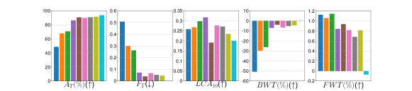
(a)

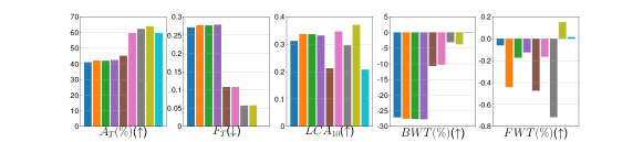
(b)

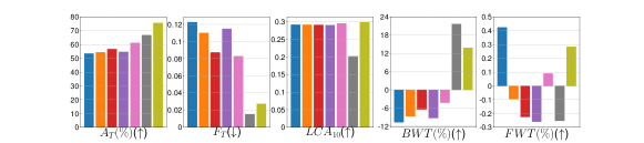
(c)

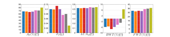
(d)

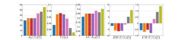
(e)

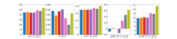
(f)

(g)

Figure 2: Models evaluated on Permuted MNIST, Split CIFAR, Split CUB, Split CUB(-JE), Split AWA and Split AWA(-JE); the models are trained over 5 runs.

4.2 Baselines

The baselines and state-of-the-art approaches can be classified into (i) training the model without regularization or extra memory, where the parameters of the current task are initialized from the parameters of the previous task; VAN is shown in the experiments; (ii) training individual models on previous tasks and then carrying out a new stage of training a new task with models of previous tasks such as PROGNN [15]; (iii) using a regularization to slow down learning on network weights that correlate with previous acquired knowledge, such as EWC [7], PI [8], RWALK [9] and MAS [10]; (iv) using extra memory to provide the data for previous tasks in a sustained manner. A-GEM, A-A-GEM and $\epsilon$-SOFT-GEM are combinations of regularization and extra memory. In addition, a generative model [28, 29] used as extra memory is applied in continual learning as well; it is not considered in this work because it performs poorly in a single training epoch. Finally, we refer to one-hot embedding as the default, and to joint embedding [12] by appending a suffix ’-JE’ to the sequential task name, which indicates that the models are trained and evaluated on the task by adopting joint embedding.

The settings of the neural network architectures used in this paper are described in Table 2 in Appendix B. For a given sequential task, all models use the same architecture and apply stochastic gradient descent optimization with 10 for the mini-batch size; the remaining training parameters of the models are the same as in [12].

4.3 Metrics

We evaluated the model on the following metrics:

1. The average accuracy on all tasks after the $k$-th sequential task learned $A_{k}$ [11], which indicates the balance of the stability and plasticity of the model; $A_{T}$ is the average accuracy of all tasks after the last task learned; the accuracy of the first task after all sequential tasks learned $a_{1}$ and the accuracy of the last task after all sequential tasks learned $a_{t}$ are also considered.

2. The forgetting $F_{k}$ [9], which indicates the ability of the model to preserve the knowledge of previous tasks.

3. The learning curve area ($LCA\in[0,1]$) [12], which indicates the ability of the model to learn a new task.

4. Backward transfer ($BWT$) [11], which indicates the influence of the performance on previous tasks $k<t$ when the model is learning task $t$. A positive $BWT$ indicates an increase in the performance of the previous task, and a large negative $BWT$ indicates catastrophic forgetting.

5. Forward transfer ($FWT$) [11], which indicates the influence of the performance on future tasks $k>t$ when the model is learning task $t$. A positive $FWT$ shows that the model can perform “zero-shot” learning.

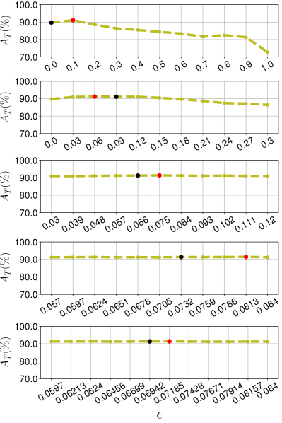
(a)

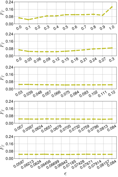
(b)

Figure 3: $\epsilon$-SOFT-GEM on Permuted MNIST in 5 training repeats, where the models are trained over 5 runs in a single training repeat.

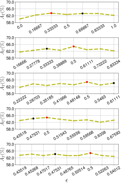
(a)

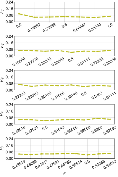
(b)

Figure 4: $\epsilon$-SOFT-GEM on Split CIFAR in 5 training repeats, where the models are trained over 5 runs in a single training repeat.

4.4 Comparison with baselines

In this section, we show the applicability of $\epsilon$-SOFT-GEM and A-A-GEM on sequential learning tasks. The details of the results are shown in Tables 3, 4, 5, 6, 7 and 8 in Appendix E.

First, Figure 2 shows that $\epsilon$-SOFT-GEM outperforms other models on Permuted MNIST, Split CIFAR, Split CUB, Split CUB(-JE), Split AWA and Split AWA(-JE), except for PROGNN, which achieves slightly better performance than $\epsilon$-SOFT-GEM on Permuted MNIST. The reason is that PROGNN trains an individual model on a previous task and then carries out a new stage of training a new task; it can preserve all the information it learned on previous tasks. Meanwhile, from the snapshot of the statistics of the datasets shown in Table 1 in Appendix A, PROGNN achieves better performance on a large-scale training sample dataset and lower performance on a smaller training sample dataset. However, PROGNN has the worst memory problem because the size of the parameters of the model increases superlinearly with the number of tasks, and it will run out of memory during training due to the large size of the model; therefore, PROGNN is invalid on Split CUB and Split AWA, which apply the standard ResNet18 in Table 2 in Appendix B, which is not shown in Figures 2(c), 2(d), 2(e) and 2(f).

Second, $\epsilon$-SOFT-GEM acquires better $a_{1}$, $a_{t}$, $A_{T}$ and $F_{T}$ values than the other baselines shown in Tables 3, 4, 5, 6, 7 and 8, which means that $\epsilon$-SOFT-GEM can maintain its performance on previous tasks when learning new tasks. $LCA_{10}$ in Figure 2 shows that $\epsilon$-SOFT-GEM has a competitive capacity to learn new knowledge fast, even compared with A-GEM.

Third, the $BWT$ values of $\epsilon$-SOFT-GEM and A-A-GEM are positive in Split CUB and Split AWA; Figure 2 shows that $\epsilon$-SOFT-GEM and A-A-GEM can learn new knowledge of previous tasks to increase the performance of the model on previous tasks, while the other baselines have a negative $BWT$ for 4 sequential learning tasks. The $FWT$ value indicates that $\epsilon$-SOFT-GEM has a competitive ability to perform “zero-shot” learning.

Fourth, from the results shown in Figure 2, A-A-GEM performs better than the other models except for $\epsilon$-SOFT-GEM, but A-A-GEM is much simpler than $\epsilon$-SOFT-GEM without specifying $\epsilon$.

Finally, we can conclude that $\epsilon$-SOFT-GEM can balance preserving the knowledge of old tasks with a soft constraint $\epsilon$ and learning new tasks with a fast learning curve.

4.5 Exploration of $\epsilon$

In this work, we use a simple heuristic algorithm to explore $\epsilon$. Each row in Figures 3 and 4 is a population trained with a specific set $\epsilon$, and there are 5 training repeats in the whole experiment.

In the first repeat, we divide $\epsilon\in[0,1]$ into $N$ equal parts with an interval $\delta$; for example, for Permuted MNIST, $N=11,\delta=0.1$, and for Split CIFAR, $N=7,\delta=0.16667$.

After the $j$-th training repeat, we choose the $\epsilon_{j,1}$ that yields the best $A_{j,T}$, the $\epsilon_{j,2}$ with the second-best $A_{j,T}$ and an interval $\delta_{j}$, where $A_{j,T}$ is $A_{T}$ after the $j$-th training repeat and $\delta_{j}$ is the interval of the $j$-th training repeat. Meanwhile, we define $\epsilon_{j}[1]$ and $\epsilon_{j}[N]$ as the smallest and largest values of $\epsilon_{j}$, respectively. We assume $\epsilon_{j,1}\leq\epsilon_{j,2}$, and the update rule of $\epsilon_{j+1}$ is:

$$\footnotesize\epsilon_{j+1}\in\left\{\begin{array}[]{l}\left[0,1\right],\quad j=0;\\ \mathrm{stop},\quad\epsilon_{j,1}=\epsilon_{j}[1],\epsilon_{j,2}=\epsilon_{j}[N]\ \mathrm{and}\ j>0\ \mathrm{or}\ j>M\\ \left[\epsilon_{j,1},\epsilon_{j,2}+\delta_{j}\right],\quad\epsilon_{j,1}=\epsilon_{j}[1]\ \mathrm{and}\ 0<j\leq M;\\ \left[\epsilon_{j,1}-\delta_{j},\epsilon_{j,2}\right],\quad\epsilon_{j,2}=\epsilon_{j}[N]\ \mathrm{and}\ 0<j\leq M;\\ \left[\epsilon_{j,1}-\delta_{j},\epsilon_{j,2}+\delta_{j}\right],\ \mathrm{other};\end{array}\right.$$ (12)

where $M$ is the number of training repeats. $\epsilon$-SOFT-GEM with $\epsilon=0.0$ is equal to A-GEM with the original $g$ and $g_{ref}$, not $\hat{g}$ and $\hat{g}_{ref}$.

The soft constraint $\epsilon$ adjusts the capacity of the model to learn new tasks and preserve old tasks. According to the update rule above, we repeat the process 5 times to explore $\epsilon$. First, the top row in Figures 3 and 4 shows that $\epsilon$-SOFT-GEM outperforms A-GEM with a specified $\epsilon$, such as $\epsilon=0.1$ in Permuted MNIST and all training populations with a specified $\epsilon$ in Split-CIFAR. Second, $A_{T}$ in every repeat is basically a parabolic curve; therefore, the heuristic optimization algorithm for exploring the best $\epsilon$ is effective. Finally, we find that $\epsilon=0.07185$ in Permuted MNIST and $\epsilon=0.5$ in Split CIFAR after 5 training repeats.

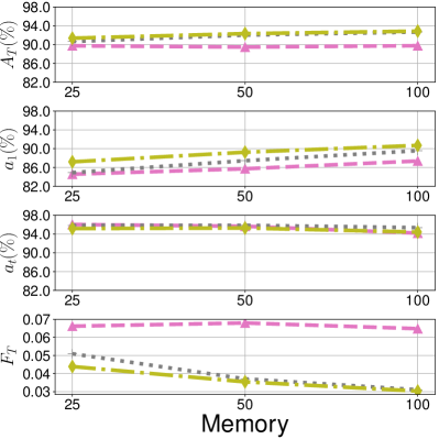
(a)

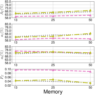
(b)

(c)

Figure 5: $A_{T}$, $a_{1}$, $a_{t}$ and $F_{T}$ on Permuted MNIST and Split CIFAR with varying episodic memory size in a single training epoch; the models are trained over 5 runs. The details are shown in Tables 9 and 10 in Appendix E.

4.6 Episodic memory

The conventional solution to catastrophic forgetting is to learn a new task alongside the old samples we preserve; the episodic memory needed to preserve the old samples is significant in A-GEM, A-A-GEM and $\epsilon$-SOFT-GEM.

Therefore, we run the experiments on A-GEM, A-A-GEM and $\epsilon$-SOFT-GEM with varying episodic memory size. $A_{T}$, $a_{1}$, $a_{t}$ and $F_{T}$ on Permuted MNIST and Split CIFAR are shown in Figure 5; $\epsilon$-SOFT-GEM outperforms A-GEM and A-A-GEM in $A_{T}$ and $F_{T}$. The reasons are: (i) the larger the episodic memory is, the more old information can be preserved; $g_{ref}$ can represent the actual gradient of the old tasks more accurately, and $\epsilon$-SOFT-GEM can preserve more of the old information, as illustrated in $a_{1}$ which is increasing; (ii) A-GEM, A-A-GEM and $\epsilon$-SOFT-GEM can learn new tasks with competitive accuracy in a training epoch with a relatively slow learning curve, which is illustrated by $a_{t}$ which is decreasing.

4.7 Efficiency

From the update rule of the gradient, $\epsilon$-SOFT-GEM and A-A-GEM have only one more gradient normalization operation than A-GEM, and we can deduce that $\epsilon$-SOFT-GEM and A-A-GEM acquire almost the same efficient computation and memory costs as A-GEM.

5 CONCLUSION

In the real world, humans can learn and accumulate knowledge throughout their whole lives, but ANNs that learn sequential tasks suffer from catastrophic forgetting, in which the learned knowledge is disrupted while a new task is being learned. To alleviate catastrophic forgetting, we propose a variant of A-GEM with a soft constraint $\epsilon$, called $\epsilon$-SOFT-GEM, as well as A-A-GEM. The experiments demonstrate that $\epsilon$-SOFT-GEM has competitive performance against state-of-the-art models. First, compared to regularization-based approaches, $\epsilon$-SOFT-GEM achieves significantly higher average accuracy and lower forgetting; additionally, it maintains a fast learning curve and can acquire new knowledge of previous tasks represented by episodic memory when learning new tasks. Second, $\epsilon$-SOFT-GEM has almost the same efficiency cost as A-GEM in terms of computation and memory. Third, A-A-GEM performs better than the other models except for $\epsilon$-SOFT-GEM, but A-A-GEM is much simpler than $\epsilon$-SOFT-GEM without specifying $\epsilon$.

Appendix A Sequential Task Statistics

The summary of the sequential tasks described above is shown in Table 1, where ‘-’ indicates that the size of the samples in each task is different.

Table 1: Sequential tasks statistics

	Permuted MNIST	Split CIFAR	Split CUB	Split AWA
tasks	$20$	$20$	$20$	$20$
input size	$28*28*1$	$32*32*3$	$224*224*3$	$224*224*3$
classes per task	$10$	$5$	$10$	$5$
training images per task	$6*10^{4}$	$2.5*10^{2}$	$3*10^{2}$	-
test images per task	$10^{4}$	$5*10^{2}$	$2.9*10^{2}$	-

Appendix B Neural Network Architecture

The settings of the neural network architectures used in the paper are described in Table 2, where memory means the episodic memory per label per task; for example, the memory capacity of each task of Permuted MNIST is $25\times 10=250$, and the total memory capacity is $250\times 20=5000$.

Table 2: The settings of the neural network architectures on sequential tasks

datasets	setting	learning rate	memory
Permuted MNIST	Fully-connected network, two hidden layers of 256 ReLU units.	0.1	25
Split CIFAR	Reduced ResNet18, same as the model described in [11].	0.03	13
Split CUB	Standard ResNet18, same as the model described in [30].	0.1	5
Split AWA	Standard ResNet18, same as the model applied on Split CUB.	0.1	20

Appendix C $\epsilon$-Soft-Gem Update Rule

The update rule of $\epsilon$-SOFT-GEM is $\widetilde{g}=\hat{g}-\frac{\hat{g}^{\mathrm{T}}\hat{g}_{ref}-\mathbf{\epsilon}}{\hat{g}_{ref}^{\mathrm{T}}\hat{g}_{ref}}\hat{g}_{ref}$.

The optimization object of $\epsilon$-SOFT-GEM is:

$$\begin{array}[]{ll}\text{minimize}_{\widetilde{g}}&\quad\frac{1}{2}||\hat{g}-\widetilde{g}||_{2}^{2}\\ \text{subject to}&\quad\widetilde{g}^{\mathrm{T}}\hat{g}_{ref}\geq\mathbf{\epsilon},\quad\epsilon\in[0,1].\end{array}$$ (13)

Replacing $\widetilde{g}$ with $z$ and rewriting (13) yields:

$$\begin{array}[]{ll}\text{minimize}_{z}&\quad\frac{1}{2}z^{\mathrm{T}}z-\hat{g}^{\mathrm{T}}z\\ \text{subject to}&\quad-z^{\mathrm{T}}\hat{g}_{ref}+\epsilon\leq 0,\quad\epsilon\in[0,1].\end{array}$$ (14)

Putting the cost function as well as the constraints in a single minimization problem, the dual optimization problem of (14) can be written as:

$$\begin{array}[]{l}\mathcal{L}(z,\alpha)=\frac{1}{2}z^{\mathrm{T}}z-\hat{g}^{\mathrm{T}}z-\alpha(z^{\mathrm{T}}\hat{g}_{ref}-\mathbf{\epsilon}),\end{array}$$ (15)

where $\alpha$ is a Lagrange multiplier.

The solution of (15) satisfies:

$$\begin{array}[]{l}\nabla_{z}\mathcal{L}(z,\alpha)=0\end{array}$$ (16)

and

$$\begin{array}[]{l}\nabla_{\alpha}\mathcal{L}(z,\alpha)=0.\end{array}$$ (17)

Consider (15) and (16),

$$\begin{array}[]{l}\nabla_{z}\mathcal{L}(z,\alpha)=z^{*}-\hat{g}-\alpha\hat{g}_{ref}=0,\end{array}$$ (18)

the solution $z^{*}$ of (18) is:

$$\begin{array}[]{l}z^{*}=\hat{g}+\alpha\hat{g}_{ref}.\end{array}$$ (19)

Now, plug $z^{*}$ into equation (15) to obtain

$$\begin{array}[]{ll}\mathcal{L}(z^{*},\alpha)&=\frac{1}{2}(\hat{g}^{\mathrm{T}}+\alpha\hat{g}_{ref}^{\mathrm{T}})(\hat{g}+\alpha\hat{g}_{ref})-\hat{g}^{\mathrm{T}}(\hat{g}+\alpha\hat{g}_{ref})-\alpha((\hat{g}^{\mathrm{T}}+\alpha\hat{g}_{ref}^{\mathrm{T}})\hat{g}_{ref}-\mathbf{\epsilon})\\ &=-\frac{1}{2}\hat{g}^{\mathrm{T}}\hat{g}-\alpha\hat{g}^{\mathrm{T}}\hat{g}_{ref}-\frac{1}{2}\alpha^{2}\hat{g}_{ref}^{\mathrm{T}}\hat{g}_{ref}+\alpha\mathbf{\epsilon}.\end{array}$$ (20)

Consider (17) and (20).

$$\begin{array}[]{l}\nabla_{\alpha}\mathcal{L}(z^{*},\alpha)=-\hat{g}^{\mathrm{T}}\hat{g}_{ref}-\alpha\hat{g}_{ref}^{\mathrm{T}}\hat{g}_{ref}+\mathbf{\epsilon}=0,\end{array}$$ (21)

the solution $\alpha^{*}$ of (21) is:

$$\begin{array}[]{l}\alpha^{*}=-\frac{\hat{g}^{\mathrm{T}}\hat{g}_{ref}-\mathbf{\epsilon}}{\hat{g}_{ref}^{\mathrm{T}}\hat{g}_{ref}}.\end{array}$$ (22)

Plugging $\alpha^{*}$ into equation (19), the SOFT-GEM update rule is obtained as:

$$\begin{array}[]{l}z^{*}=\hat{g}-\frac{\hat{g}^{\mathrm{T}}\hat{g}_{ref}-\mathbf{\epsilon}}{\hat{g}_{ref}^{\mathrm{T}}\hat{g}_{ref}}\hat{g}_{ref}=\widetilde{g}.\end{array}$$ (23)

Appendix D ALGORITHMS

The algorithm for $\epsilon$-SOFT-GEM and A-A-GEM is illustrated in Algorithm 1, and the evaluation (EVAL) and update episodic memory (UPDATAEPSMEM) procedures are introduced from [12].

Algorithm 1 Training and evaluation of $\epsilon$-SOFT-GEM and A-A-GEM on sequential data $\mathcal{D}=\{\mathcal{D}_{1},...,\mathcal{D}_{T}\}$

procedure $\epsilon$-SOFT-GEM($\epsilon$, $f_{\theta},\mathcal{D}^{train},\mathcal{D}^{test}$)

     $\mathcal{M}\leftarrow\{\}$

     $A\leftarrow 0\in\mathbb{R}^{\text{T}\times\text{T}}$

     for t = {1, …, T} do

         for $(\mathbf{x},y)\in\mathcal{D}_{t}^{train}$ do

              $(\mathbf{x}_{ref},y_{ref})\sim\mathcal{M}$

              $g_{ref}\leftarrow\nabla_{\theta}l(f_{\theta}(\mathbf{x}_{ref},t),y_{ref})$

              $g\leftarrow\nabla_{\theta}l(f_{\theta}(\mathbf{x},t),y)$

              $\hat{g}\leftarrow\frac{g}{|g|}$ ,$\hat{g}_{ref}\leftarrow\frac{g_{ref}}{|g_{ref}|}$ $\triangleright$ Normalize $g$ and $g_{ref}$

              if $\hat{g}^{T}\hat{g}_{ref}\geq 0$ then

                  $\widetilde{g}\leftarrow g$

              else

                  if $\epsilon$-SOFT-GEM then

                       $\widetilde{g}\leftarrow\hat{g}-\frac{{{\hat{g}^{\text{T}}}}\hat{g}_{ref}-\epsilon}{{{\hat{g}_{ref}^{\text{T}}}}\hat{g}_{ref}}\hat{g}_{ref}$ $\triangleright$ $\epsilon$-SOFT-GEM update rule

                  else if A-A-GEM then

                       $\widetilde{g}\leftarrow\frac{\hat{g}+\hat{g}_{ref}}{2}$ $\triangleright$ A-A-GEM update rule

                  end if

              end if

              $\theta\leftarrow\theta-\alpha\widetilde{g}$

         end for

         $M\leftarrow\mathrm{UPDATAEPSMEM}(\mathcal{M},\mathcal{D}_{t}^{train},T)$ $\triangleright$ Update the episodic memory

         $A_{t,:}\leftarrow\mathrm{EVAL}(f_{\theta},\mathcal{D}^{test})$ $\triangleright$ Evaluate the model

     end for

return $f_{\theta},A$

end procedure

Appendix E RESULTS

Table 3: Models on Permuted MNIST

Methods	Permuted MNIST
	$A_{T}(\%)(\uparrow)$	$F_{T}(\downarrow)$	$a_{1}(\%)(\uparrow)$	$a_{t}(\%)(\uparrow)$	$FWT(\%)(\uparrow)$	$BWT(\%)(\uparrow)$
VAN	$48.6(\pm 1.28)$	$0.21(\pm 0.013)$	$21.1(\pm 2.81)$	$96.2(\pm 0.22)$	$1.12(\pm 0.403)$	$-50.68(\pm 1.342)$
EWC	$67.6(\pm 1.83)$	$0.30(\pm 0.019)$	$42.8(\pm 4.48)$	$95.8(\pm 0.20)$	$1.06(\pm 0.420)$	$-29.84(\pm 1.906)$
MAS	$70.7(\pm 1.29)$	$0.26(\pm 0.013)$	$45.2(\pm 3.86)$	$95.3(\pm 0.25)$	$\bm{1.14(\pm 0.523)}$	$-26.06(\pm 1.361)$
RWALK	$86.3(\pm 1.00)$	$0.07(\pm 0.009)$	$93.2(\pm 0.67)$	$92.2(\pm 0.99)$	$0.84(\pm 0.488)$	$-6.94(\pm 0.935)$
ER	$90.6(\pm 0.07)$	$0.04(\pm 0.001)$	$91.6(\pm 0.45)$	$94.2(\pm 0.15)$	$0.94(\pm 0.159)$	$-3.83(\pm 0.068)$
A-GEM	$89.8(\pm 0.32)$	$0.07(\pm 0.003)$	$84.6(\pm 0.42)$	$\bm{96.0(\pm 0.28)}$	$0.82(\pm 0.383)$	$-6.60(\pm 0.338)$
A-A-GEM	$90.7(\pm 0.20)$	$0.05(\pm 0.001)$	$85.0(\pm 0.72)$	$95.8(\pm 0.07)$	$0.68(\pm 0.178)$	$-5.09(\pm 0.190)$
$\epsilon$-SOFT-GEM	$91.3(\pm 0.11)$	$0.05(\pm 0.001)$	$87.2(\pm 0.32)$	$95.1(\pm 0.28)$	$0.81(\pm 0.414)$	$-4.49(\pm 0.123)$
PROGNN	$\bm{93.5(\pm 0.10)}$	$\bm{0(\pm 0)}$	$\bm{96.2(\pm 0.27)}$	$90.9(\pm 0.55)$	$-0.07(\pm 0.817)$	$\bm{0(\pm 0)}$

Table 4: Models on Split CIFAR

Methods	Split CIFAR
	$A_{T}(\%)(\uparrow)$	$F_{T}(\downarrow)$	$a_{1}(\%)(\uparrow)$	$a_{t}(\%)(\uparrow)$	$FWT(\%)(\uparrow)$	$BWT(\%)(\uparrow)$
VAN	$40.9(\pm 4.38)$	$0.27(\pm 0.040)$	$31.4(\pm 8.61)$	$71.4(\pm 4.58)$	$-0.06(\pm 1.570)$	$-27.07(\pm 4.037)$
EWC	$41.8(\pm 4.02)$	$0.28(\pm 0.041)$	$26.6(\pm 6.94)$	$75.8(\pm 4.19)$	$-0.44(\pm 0.871)$	$-27.5(\pm 4.179)$
MAS	$41.8(\pm 4.73)$	$0.28(\pm 0.042)$	$22.8(\pm 6.94)$	$72.8(\pm 7.86)$	$-0.17(\pm 0.611)$	$-27.6(\pm 4.191)$
RWALK	$42.2(\pm 4.80)$	$0.28(\pm 0.042)$	$29.5(\pm 7.56)$	$\bm{76.6(\pm 4.88)}$	$-0.12(\pm 0.580)$	$-27.7(\pm 4.307)$
ER	$45.0(\pm 2.27)$	$0.11(\pm 0.009)$	$47.4(\pm 8.94)$	$54.8(\pm 9.04)$	$-0.47(\pm 0.978)$	$-10.6(\pm 0.821)$
A-GEM	$58.6(\pm 3.67)$	$0.11(\pm 0.034)$	$56.1(\pm 11.45)$	$76.0(\pm 4.00)$	$-0.16(\pm 1.118)$	$-10.2(\pm 3.193)$
A-A-GEM	$62.1(\pm 1.97)$	$0.06(\pm 0.010)$	$61.1(\pm 8.67)$	$69.8(\pm 6.30)$	$-0.72(\pm 0.853)$	$-3.02(\pm 1.295)$
$\epsilon$-SOFT-GEM	$\bm{63.9(\pm 1.53)}$	$0.06(\pm 0.014)$	$60.1(\pm 9.21)$	$75.1(\pm 5.54)$	$\bm{0.15(\pm 1.156)}$	$-3.69(\pm 0.797)$
PROGNN	$59.6(\pm 0.92)$	$\bm{0(\pm 0)}$	$\bm{64.6(\pm 7.14)}$	$65.8(\pm 5.45)$	$0.01(\pm 0.525)$	$\bm{0(\pm 0)}$

Table 5: Models on Split CUB with one-hot. ’OoM’ in the table means that the model fails to fit within the memory.

Methods	Split CUB
	$A_{T}(\%)(\uparrow)$	$F_{T}(\downarrow)$	$a_{1}(\%)(\uparrow)$	$a_{t}(\%)(\uparrow)$	$FWT(\%)(\uparrow)$	$BWT(\%)(\uparrow)$
VAN	$53.4(\pm 0.76)$	$0.12(\pm 0.030)$	$34.5(\pm 7.66)$	$64.9(\pm 7.00)$	$\bm{0.42(\pm 0.93})$	$-10.71(\pm 3.354)$
EWC	$54.3(\pm 1.73)$	$0.11(\pm)0.015$	$37.1(\pm 8.21)$	$64.8(\pm 11.25)$	$-0.09(\pm 1.04)$	$-8.69(\pm 2.360)$
PI	$56.6(\pm 2.91)$	$0.09(\pm)0.005$	$40.2(\pm 7.35)$	$69.3(\pm 10.36)$	$-0.22(\pm 0.57)$	$-6.41(\pm 1.125)$
RWALK	$54.5(\pm 1.50)$	$0.11(\pm 0.016)$	$34.8(\pm 8.35)$	$70.0(\pm 7.58)$	$-0.26(\pm 0.93)$	$-9.26(\pm 2.434)$
A-GEM	$61.1(\pm 3.12)$	$0.08(\pm 0.012)$	$56.6(\pm 5.81)$	$69.6(\pm 6.83)$	$0.09(\pm 0.33)$	$-4.19(\pm 2.384)$
A-A-GEM	$66.7(\pm 2.40)$	$\bm{0.02(\pm 0.015)}$	$\bm{73.9(\pm 5.50)}$	$54.7(\pm 10.80)$	$-0.25(\pm 0.34)$	$\bm{21.70(\pm 2.083)}$
$\epsilon$-SOFT-GEM	$\bm{75.6(\pm 2.00)}$	$0.03(\pm 0.009)$	$73.3(\pm 4.95)$	$\bm{70.7(\pm 5.52)}$	$0.28(\pm 0.98)$	$13.79(\pm 2.979)$
PROGNN	OoM	OoM	OoM	OoM	OoM	OoM

Table 6: Models on Split CUB with joint embedding. ’OoM’ in the table means that the model fails to fit within the memory.

Methods	Split CUB(-JE)
	$A_{T}(\%)(\uparrow)$	$F_{T}(\downarrow)$	$a_{1}(\%)(\uparrow)$	$a_{t}(\%)(\uparrow)$	$FWT(\%)(\uparrow)$	$BWT(\%)(\uparrow)$
VAN	$67.7(\pm 5.40)$	$0.10(\pm 0.057)$	$58.1(\pm 10.39)$	$79.3(\pm 5.34)$	$32.47(\pm 2.867)$	$-5.75(\pm 5.758)$
EWC	$67.5(\pm 4.61)$	$0.10(\pm 0.043)$	$57.6(\pm 9.41)$	$79.6(\pm 4.99)$	$31.6(\pm 2.530)$	$-5.41(\pm 4.814)$
PI	$65.8(\pm 5.71)$	$0.11(\pm 0.068)$	$54.6(\pm 8.80)$	$78.1(\pm 4.43)$	$32.19(\pm 2.616)$	$-7.24(\pm 6.758)$
RWALK	$67.1(\pm 4.20)$	$0.10(\pm 0.041)$	$58.1(\pm 9.10)$	$79.5(\pm 5.60)$	$32.04(\pm 1.976)$	$-5.77(\pm 3.464)$
A-GEM	$71.1(\pm 3.59)$	$0.08(\pm 0.020)$	$64.3(\pm 10.27)$	$81.2(\pm 6.99)$	$34.92(\pm 2.585)$	$-4.23(\pm 1.605)$
A-A-GEM	$70.1(\pm 2.40)$	$0.08(\pm 0.028)$	$68.2(\pm 5.73)$	$77.0(\pm 4.58)$	$35.61(\pm 2.697)$	$-2.80(\pm 2.954)$
$\epsilon$-SOFT-GEM	$\bm{79.8(\pm 2.73)}$	$\bm{0.03(\pm 0.021)}$	$\bm{80.2(\pm 6.25)}$	$\bm{82.7(\pm 4.55)}$	$\bm{36.71(\pm 2.432)}$	$\bm{6.54(\pm 2.639)}$
PROGNN	OoM	OoM	OoM	OoM	OoM	OoM

Table 7: Models on Split AWA with one-hot. ’OoM’ in the table means that the model fails to fit within the memory.

Methods	Split AWA
	$A_{T}(\%)(\uparrow)$	$F_{T}(\downarrow)$	$a_{1}(\%)(\uparrow)$	$a_{t}(\%)(\uparrow)$	$FWT(\%)(\uparrow)$	$BWT(\%)(\uparrow)$
VAN	$29.4(\pm 2.65)$	$0.03(\pm 0.008)$	$26.8(\pm 5.01)$	$34.2(\pm 8.60)$	$-0.56(\pm 1.218)$	$-2.09(\pm 0.781)$
EWC	$33.7(\pm 3.52)$	$0.07(\pm 0.017)$	$27.9(\pm 4.16)$	$43.3(\pm 7.64)$	$-0.68(\pm 0.630)$	$-5.83(\pm 1.796)$
PI	$33.5(\pm 3.65)$	$0.07(\pm 0.017)$	$28.4(\pm 4.39)$	$43.6(\pm 7.64)$	$-0.52(\pm 0.641)$	$-6.33(\pm 1.575)$
RWALK	$33.7(\pm 3.17)$	$0.07(\pm 0.020)$	$29.1(\pm 5.07)$	$43.5(\pm 6.81)$	$-0.78(\pm 0.459)$	$-6.05(\pm 2.049)$
A-GEM	$43.0(\pm 3.24)$	$0.05(\pm 0.015)$	$42.8(\pm 7.53)$	$45.0(\pm 5.58)$	$0.33(\pm 1.088)$	$-0.97(\pm 0.856)$
A-A-GEM	$46.3(\pm 3.64)$	$0.02(\pm 0.027)$	$47.3(\pm 9.36)$	$39.2(\pm 7.58)$	$0.91(\pm 1.443)$	$5.19(\pm 2.542)$
$\epsilon$-SOFT-GEM	$\bm{55.3(\pm 3.57)}$	$\bm{0.01(\pm 0.028)}$	$\bm{53.4(\pm 8.88)}$	$\bm{45.3(\pm 7.99)}$	$\bm{1.38(\pm 1.453)}$	$\bm{10.65(\pm 2.051)}$
PROGNN	OoM	OoM	OoM	OoM	OoM	OoM

Table 8: Models on Split AWA with joint embedding. ’OoM’ in the table means that the model fails to fit within the memory.

Methods	Split AWA (-JE)
	$A_{T}(\%)(\uparrow)$	$F_{T}(\downarrow)$	$a_{1}(\%)(\uparrow)$	$a_{t}(\%)(\uparrow)$	$FWT(\%)(\uparrow)$	$BWT(\%)(\uparrow)$
VAN	$44.3(\pm 3.05)$	$0.05(\pm 0.015)$	$39.9(\pm 2.30)$	$51.7(\pm 3.83)$	$11.65(\pm 1.677)$	$-0.93(\pm 1.575)$
EWC	$45.1(\pm 2.61)$	$0.04(\pm 0.011)$	$40.5(\pm 3.45)$	$50.5(\pm 5.07)$	$11.81(\pm 1.930)$	$0.19(\pm 0.992)$
PI	$43.7(\pm 3.53)$	$0.05(\pm 0.015)$	$40.7(\pm 3.98)$	$48.6(\pm 3.78)$	$12.26(\pm 1.892)$	$0.03(\pm 1.024)$
RWALK	$44.0(\pm 2.75)$	$0.05(\pm 0.012)$	$39.9(\pm 2.68)$	$44.0(\pm 3.53)$	$12.00(\pm 1.938)$	$-1.42(\pm 1.537)$
A-GEM	$48.4(\pm 2.58)$	$0.03(\pm 0.007)$	$49.6(\pm 7.65)$	$\bm{49.7(\pm 4.54)}$	$15.19(\pm 1.591)$	$2.60(\pm 1.191)$
A-A-GEM	$47.2(\pm 2.20)$	$\bm{0.02(\pm 0.008)}$	$48.0(\pm 5.60)$	$48.8(\pm 3.16)$	$14.68(\pm 1.035)$	$4.53(\pm 1.217)$
$\epsilon$-SOFT-GEM	$\bm{53.5(\pm 5.07)}$	$0.04(\pm 0.038)$	$\bm{54.6(\pm 7.73)}$	$48.7(\pm 6.81)$	$\bm{20.22(\pm 1.698)}$	$\bm{6.30(\pm 3.682)}$
PROGNN	OoM	OoM	OoM	OoM	OoM	OoM

Table 9: Permuted MNIST with varying episodic memory size

Methods		A-GEM	A-A-GEM	$\epsilon$-SOFT-GEM
$A_{T}(\%)(\uparrow)$	25	$89.6(\pm 0.32)$	$90.7(\pm 0.20)$	$\bm{91.3(\pm 0.11)}$
	50	$89.5(\pm 0.04)$	$92.0(\pm 0.09)$	$\bm{92.3(\pm 0.15)}$
	100	$89.8(\pm 0.45)$	$92.7(\pm 0.11)$	$\bm{92.9(\pm 0.08)}$
$a_{1}(\%)(\uparrow)$	25	$84.6(\pm 0.43)$	$85.0(\pm 0.72)$	$\bm{87.2(\pm 0.32)}$
	50	$85.7(\pm 1.05)$	$87.5(\pm 0.33)$	$\bm{89.3(\pm 0.60)}$
	100	$87.4(\pm 1.17)$	$89.6(\pm 0.32)$	$\bm{90.7(\pm 0.34)}$
$a_{t}(\%)(\uparrow)$	25	$\bm{96.0(\pm 0.25)}$	$95.8(\pm 0.07)$	$95.1(\pm 0.28)$
	50	$95.6(\pm 0.19)$	$\bm{95.8(\pm 0.17)}$	$95.3(\pm 0.18)$
	100	$94.2(\pm 0.47)$	$\bm{95.3(\pm 0.18)}$	$94.4(\pm 0.50)$
$F_{T}(\downarrow)$	25	$0.07(\pm 0.003)$	$0.05(\pm 0.001)$	$\bm{0.05(\pm 0.001)}$
	50	$0.07(\pm 0.001)$	$0.04(\pm 0.001)$	$\bm{0.04(\pm 0.001)}$
	100	$0.06(\pm 0.004)$	$0.03(\pm 0.001)$	$\bm{0.03(\pm 0.001)}$

Table 10: Split CIFAR with varying episodic memory size

Methods		A-GEM	A-A-GEM	$\epsilon$-SOFT-GEM
$A_{T}(\%)(\uparrow)$	13	$58.6(\pm 3.67)$	$62.1(\pm 1.97)$	$\bm{63.9(\pm 1.53)}$
	25	$60.8(\pm 1.47)$	$65.0(\pm 1.09)$	$\bm{66.4(\pm 2.07)}$
	50	$62.0(\pm 2.00)$	$67.2(\pm 1.95)$	$\bm{69.3(\pm 1.76)}$
$a_{1}(\%)(\uparrow)$	13	$56.1(\pm 11.45)$	$\bm{61.1(\pm 8.67)}$	$60.1(\pm 9.21)$
	25	$61.3(\pm 7.95)$	$\bm{66.2(\pm 6.47)}$	$64.0(\pm 7.03)$
	50	$60.4(\pm 8.86)$	$67.0(\pm 8.22)$	$\bm{68.5(\pm 5.05)}$
$a_{t}(\%)(\uparrow)$	13	$\bm{76.0(\pm 4.00)}$	$69.8(\pm 6.30)$	$75.1(\pm 6.54)$
	25	$74.6(\pm 7.94)$	$74.2(\pm 4.17)$	$\bm{74.9(\pm 8.58)}$
	50	$73.4(\pm 4.66)$	$71.7(\pm 6.76)$	$\bm{73.4(\pm 3.97)}$
$F_{T}(\downarrow)$	13	$0.11(\pm 0.034)$	$0.06(\pm 0.010)$	$\bm{0.06(\pm 0.014)}$
	25	$0.10(\pm 0.013)$	$\bm{0.04(\pm 0.008)}$	$0.05(\pm 0.020)$
	50	$0.09(\pm 0.023)$	$\bm{0.03(\pm 0.010)}$	$0.03(\pm 0.019)$

References

- [1] J. L. McClelland and B. L. McNaughton. Why there are complementary learning systems in the hippocampus and neocortex: Insights from the successes and failures of connectionist models of learning and memory. Psychnlogical Review, 102(3):419–457, 1995.
- [2] Michael Mccloskey and Neal J. Cohen. Catastrophic interference in connectionist networks: The sequential learning problem. Psychology of Learning and Motivation, 24:109–165, 1989.
- [3] Roger Ratcliff. Connectionist models of recognition memory: Constraints imposed by learning and forgetting functions. Psychological Review, 97(2):285–308, 1990.
- [4] D. Hassabis, D. Kumargan, C. Summerfield, and M. Botvinick. Neuroscience-inspired artificial intelligence. Neuron Review, 95(2):245–258, 2017.
- [5] Mark Bishop Ring. Continual learning in reinforcement environments. PhD thesis, University of Texas at Austin, 1994.
- [6] Sebastian Thrun and Tom M.Mitchell. Lifelong robot learning. Robotics and Autonomous System, 15(1-2):25–46, 1995.
- [7] J. Kirkpatrick, R. Pascanu, N. C. Rabinowitz, J. Veness, G. Desjardins, A. A. Rusu, K. Milan, J. Quan, T. Ramalho, A. Grabska-Barwinska, D. Hassabis, C. Clopath, D. Kumaran, and R. Hadsell. Overcoming catastrophic forgetting in neural networks. In Proceedings of the National Academy of Sciences of the United States of America, volume 114 13, pages 3521–3526, 2017.
- [8] Friedemann Zenke, Ben Poole, and Surya Ganguli. Continual learning through synaptic intelligence. In Proceedings of the 34th International Conference on Machine Learning (ICML 17), volume 70, pages 3987–3995, 2017.
- [9] Arslan Chaudhry, Puneet Kumar Dokania, Thalaiyasingam Ajanthan, and Philip H. S. Torr. Riemannian walk for incremental learning: Understanding forgetting and intransigence. In European Conference on Computer Vision 2018 (ECCV 2018), Munich, German, 2018. Springer, Cham.
- [10] Rahaf Aljundi, Francesca Babiloni, Mohamed Elhoseiny, Marcus Rohrbach, and Tinne Tuytelaars. Memory aware synapses: Learning what (not) to forget. In European Conference on Computer Vision 2018 (ECCV 2018), Munich, German, 2018. Springer, Cham.
- [11] David Lopez-Paz and Marc' Aurelio Ranzato. Gradient episodic memory for continual learning. In 31st Conference on Neural Information Processing System (NIPS 2017), Long Beach, CA, USA, 2017.
- [12] Arslan Chaudhry, Marc’Aurelio Ranzato, Marcus Rohrbach, and Mohamed Elhoseiny. Efficient lifelong learning with A-GEM. In International Conference on Learning Representations 2019 (ICLR 2019), 2019.
- [13] A. Robins. Catastrophic forgetting in neural networks: the role of rehearsal mechanisms. In Proc. 1993 The First New Zealand International Two-Stream Conference on Artificial Neural Networks and Expert Systems, pages 65–68, Dunedin, NZL, Nov 1990.
- [14] A. Robins. Catastrophic forgetting, rehearsal and pseudorehearsal. Connection Science, 7(2):123–146, 1995.
- [15] Andrei A. Rusu, Neil C. Rabinowitz, Guillaume Desjardins, Hubert Soyer, James Kirkpatrick, Koray Kavukcuoglu, Razvan Pascanu, and Raia Hadsell. Progressive neural networks. arXiv, abs/1606.04671, 2016.
- [16] J. Yoon, E. Yang, J. LEE, and S. J. Hwang. Lifelong learning with dynamically expandable networks. In ICLR, Vancouver, CA, 2018.
- [17] G. E. Hinton, N. Srivastava, A. Krizhevsky, I. Sutskever, and R. R. Salakhutdinov. Improving neural networks by preventing co-adaptation of feature detectors. arXiv, https://arxiv.org/abs/1207.0580, 2017.
- [18] X. Glorot, A. Bordes, and Y. Bengio. Deep sparse rectifier neural networks. In JMLR, Proc. AISTATS, PMLR, volume 15, pages 315–323, 2011.
- [19] I. J. Goodfellow, D. Warde-Farley, M. Mirza, A. Courville, and Y. Bengio. Maxout networks. In Proc. PMLR, volume 28(3), pages 1319–1327, 2013.
- [20] Ian J. Goodfellow, Mehdi Mirza, Xia Da, Aaron C. Courville, and Yoshua Bengio. An empirical investigation of catastrophic forgeting in gradient-based neural networks. In Proceedings of International Conference on Learning Representations 2014 (ICLR 2014), 2014.
- [21] Sylvestre-Alvise Rebuffi, Alexander Kolesnikov, and Christoph H. Lampert. icarl: Incremental classifier and representation learning. In 2017 IEEE Conference on Computer Vision and Pattern Recognition (CVPR 2017), pages 5533–5542, 2017.
- [22] Arslan Chaudhry, Marcus Rohrbach, Mohamed Elhoseiny, Thalaiyasingam Ajanthan, Puneet Kumar Dokania, Philip H. S. Torr, and Marc’Aurelio Ranzato. Continual learning with tiny episodic memories. arXiv, abs/1902.10486, 2019.
- [23] Matthew Riemer, Ignacio Cases, Robert Ajemian, Miao Liu, Irina Rish, Yuhai Tu, and Gerald Tesauro. Learning to learn without forgetting by maximizing transfer and minimizing interference. In Proceedings of International Conference on Learning Representations 2019 (ICLR 2019), 2019.
- [24] Y. Lecun, L. Bottou, Y. Bengio, and P. Haffner. Gradient-based learning applied to document recognition. Proceedings of the IEEE, 86(11):2278–2324, 1998.
- [25] A Krizhevsky and G Hinton. Learning multiple layers of features from tiny images. Technical report, Computer Science Department, University of Toronto, Toronto, Ontario, Canada, 2009.
- [26] C. Wah, S. Branson, P. Welinder, P. Perona, and S. J. Belongie. The caltech-ucsd birds-200-2011 dataset. Technical report, California Institute of Technology, 2011.
- [27] C. H. Lampert, H. Nickisch, and S. Harmeling. Learning to detect unseen object classes by between-class attribute transfer. In CVPR, pages 951–958, Miami, FL, 2009.
- [28] H. Shin, J. K. Lee, J. Kim, and J. Kim. Continual learning with deep generative replay. In NIPS, volume 30, pages 2990–2999, Long Beach, CA, USA, 2017.
- [29] N. Kamra, U. Gupta, and Y. Liu. Deep generative dual memory network for continual learning. arXiv, https://arxiv.org/pdf/1710.10368.pdf, 2018.
- [30] Kaiming He, Xiangyu Zhang, Shaoqing Ren, and Jian Sun. Deep residual learning for image recognition. In 2016 IEEE Conference on Computer Vision and Pattern Recognition (CVPR 2016), pages 770–778, 2016.