Unified Composite Distribution and Its Applications to Double Shadowed $\alpha-\kappa-\mu$ Fading Channels

Hussien Al-Hmood,Β  and H. S. Al-Raweshidy Manuscript received November 00, 2020.The authors are with the Department of Electronic and Computer Engineering, College of Engineering, Design and Physical Sciences, Brunel University London, UK, e-mail: Hussien.Al-Hmood@brunel.ac.uk, Hamed.Al-Raweshidy@brunel.ac.uk.
Abstract

In this paper, we propose a mixture Gamma shadowed (MGS) distribution as a unified composite model via representing the shadowing by an inverse Nakagami-$m$. Accordingly, the exact expression and the asymptotic behaviour at high average signal-to-noise ratio (SNR) regime of the fundamental statistics of a MGS distribution are derived first. These statistics are then applied to analyze the performance of the wireless communications systems over double shadowed $\alpha-\kappa-\mu$ fading via providing the outage probability (OP), the average bit error probability (ABEP), the average channel capacity (ACC), and the effective capacity (EC). The average area under the receiver operating characteristics curve (AUC) of energy detection (ED) is also analyzed. The numerical and simulation results are presented to verify the validation of our analysis.

Index Terms:
Mixture Gamma distribution, average bit error probability, channel capacity, effective capacity , double shadowed $\alpha-\kappa-\mu$ fading.

I Introduction

The wireless communications channel may undergo the effect of the multipath and shadowing fading simultaneously [1]. Accordingly, many works have been recently dedicated to analyse the performance of the generalized composite models, such as, $\kappa-\mu$, $\eta-\mu$, and $\alpha-\mu$ distributions that are used to model the line-of-sight (LoS), the non-LoS (NLoS), and the non-linear wireless communication mediums, respectively [2], [3]. These generalized conditions can provide close results to the practical measurements and approximately comprise all the classical fading distributions, i.e., Rayleigh, Nakagami-$m$, Nakagami-$n$, Nakagami-$q$, one-sided Gaussian, Weibull, and Gamma. Hence, the probability density function (PDF), the cumulative distribution function (CDF), and the moment generating function (MGF) of the composite $\eta-\mu$/Gamma fading models were derived in [4]. The authors in [5] assumed that both $\kappa-\mu$ and $\eta-\mu$ fading conditions are shadowed by an inverse Gamma distribution. The fundamental statistics of the $\kappa-\mu$ shadowed fading in which the shadowing effect is represented by a Nakagami-$m$ distribution were given in [6] with applications to the outage probability (OP) and the average bit error probability (ABEP) of wireless communications systems. The composite of the $\alpha-\kappa-\mu$/Gamma distribution was analysed in [7]. The non-linear scenario of the Fisher-Snedecor $\mathcal{F}$ distribution [8], namely, $\alpha-\mathcal{F}$, was investigated in [9]. The PDF, the CDF, and the MGF of the $\alpha-\eta-\mathcal{F}$ and the $\alpha-\kappa-\mathcal{F}$ composite fading conditions were derived in [10]. These models were then unified in a single distribution which is named $\alpha-\eta-\kappa-\mathcal{F}$ composite fading [11].

Although different statistical properties have been reported in [4]-[11], they are derived in mathematically intractable expressions. This is because they are expressed in terms of either the hypergeometric or the modified Bessel functions. Therefore, the mathematical intricacy of the performance metrics of the wireless communications systems is high and this would to unclear insights into the system behaviour with the fading parameters. Moreover, this complexity is increased when the generalised multipath fading channels undergo to double shadowing impacts [12].

To overcome the aforementioned challenges, a mixture Gamma (MG) distribution has been widely used to approximate with high accuracy most of the composite generalised/Gamma fading conditions [13]-[16]. For instance, the average area under the receiver operating characteristics (AUC) curve of the energy detection (ED) based spectrum sensing was derived in [14]. The average channel capacity (ACC) of $\alpha-\eta-\lambda-\mu$/Gamma fading and the effective capacity (EC) of $\alpha-\eta-\mu$/Gamma fading were analyzed in [15] and [16], respectively, using a MG distribution.

Based on the above observations and motivated by the merits of a MG distribution, we propose a mixture Gamma shadowed (MGS) as a unified composite model where the shadowing is represented by an inverse Nakagami-$m$. To this end, the basic statistics of this distribution are mathematically simple and tractable. Consequently, a clear insight into the effects of the fading parameters on the performance of the wireless communications systems can be deduced when the channel is subjected to double shadowing impacts.

Our main contributions are summarized as follows:

  • β€’

    The exact and the asymptotic expressions at high average signal-to-noise ratio (SNR) values for novel unified mathematically tractable statistical characterizations of composite model that is based on MG and inverse Nakagami-$m$ distributions, namely, MGS distribution, are derived.

  • β€’

    The derived statistics are employed to analyse the performance of the double shadowed $\alpha-\kappa-\mu$ fading channel in which the first and the second shadowing impacts are respectively followed the Nakagami-$m$ and the inverse Nakagami-$m$ distributions. Accordingly, the equivalent parameters of a MG distribution of composite $\alpha-\kappa-\mu$/Nakagami-$m$ fading channels are provided.

  • β€’

    Capitalizing on the above, unified closed-form expressions for the ABEP, the ACC, the EC, and the average AUC are obtained.

II MG and Inverse Nakagami-$m$ Distributions

The PDF of a MG distribution is given by [13, eq. (1)]

$\displaystyle f(x)=\sum_{j=1}^{K}\sigma_{j}x^{\beta_{j}-1}e^{-\zeta_{j}x}$ (1)

where $\sigma_{j}$, $\beta_{j}$, and $\zeta_{j}$ are the parameters of $j$th Gamma component and $K$ that stands for the number of terms is evaluated via using the mean square error (MSE) method between the exact PDF and its MG representation [13].

If $\xi$ is an inverse Nakagami-$m$ random variable (RV), its PDF is expressed as [12, eq. (50)]

$\displaystyle f_{\xi}(r)=\frac{(m_{s}-1)^{m_{s}}}{\Gamma(m_{s})}r^{m_{s}-1}e^{-\frac{(m_{s}-1)}{r}}.\quad m_{s}>1$ (2)

where mssubscriptπ‘šπ‘ m_{s} refers to the shadowing severity index and $\Gamma(.)$ is the incomplete Gamma function [17, eq. (8.310.1)].

III Statistical Properties of a MGS Distribution

Let γ∼MGS​(Οƒj,Ξ²j,ΞΆj,ms)similar-to𝛾MGSsubscriptπœŽπ‘—subscript𝛽𝑗subscriptπœπ‘—subscriptπ‘šπ‘ \gamma\sim\text{MGS}(\sigma_{j},\beta_{j},\zeta_{j},m_{s}) for $j=1,\cdots,K$ is an MGS-distributed RV. Then, the PDF of $\gamma$ can be obtained by the product of MG and inverse Nakagami-$m$ RVs as [4, eq. (8)]

$\displaystyle f_{\gamma}(\gamma)=\int_{0}^{\infty}\frac{1}{z}f\bigg{(}\frac{\gamma}{z}\bigg{)}f_{\xi}(z)dz.$ (3)

Substituting (1) and (2) into (3) and making use of [17, eq. (3.381.4)] with some mathematical manipulations, this yields

fγ​(Ξ³)=(msβˆ’1)msβ€‹βˆ‘j=1KΟƒj​(ms)Ξ²j​γβjβˆ’1(msβˆ’1+ΞΆj​γ)Ξ²j+ms.subscript𝑓𝛾𝛾superscriptsubscriptπ‘šπ‘ 1subscriptπ‘šπ‘ superscriptsubscript𝑗1𝐾subscriptπœŽπ‘—subscriptsubscriptπ‘šπ‘ subscript𝛽𝑗superscript𝛾subscript𝛽𝑗1superscriptsubscriptπ‘šπ‘ 1subscriptπœπ‘—π›Ύsubscript𝛽𝑗subscriptπ‘šπ‘ \displaystyle f_{\gamma}(\gamma)=(m_{s}-1)^{m_{s}}\sum_{j=1}^{K}\frac{\sigma_{j}(m_{s})_{\beta_{j}}\gamma^{\beta_{j}-1}}{(m_{s}-1+\zeta_{j}\gamma)^{\beta_{j}+m_{s}}}. (4)

where $(.)_{n}$ is the Pochhammer symbol.

When $\zeta_{j}\rightarrow 0$ for all $j=1,\cdots,K$, the asymptotic of the PDF, $f^{\infty}_{\gamma}(\gamma)$, can be expressed as

fΞ³βˆžβ€‹(Ξ³)β‰ƒβˆ‘j=1KΟƒj​(ms)Ξ²j​γβjβˆ’1(msβˆ’1)Ξ²j.similar-to-or-equalssubscriptsuperscript𝑓𝛾𝛾superscriptsubscript𝑗1𝐾subscriptπœŽπ‘—subscriptsubscriptπ‘šπ‘ subscript𝛽𝑗superscript𝛾subscript𝛽𝑗1superscriptsubscriptπ‘šπ‘ 1subscript𝛽𝑗\displaystyle f^{\infty}_{\gamma}(\gamma)\simeq\sum_{j=1}^{K}\frac{\sigma_{j}(m_{s})_{\beta_{j}}\gamma^{\beta_{j}-1}}{(m_{s}-1)^{\beta_{j}}}. (5)

Inserting (4) in $F_{\gamma}(\gamma)=\int_{0}^{\gamma}f_{\gamma}(\gamma)d\gamma$ and recalling [17, eq. (3.194.1)], the CDF of a MGS distribution can be derived as

$\displaystyle F_{\gamma}(\gamma)=$ βˆ‘j=1KΟƒj​(ms)Ξ²j​F12​(Ξ²j+ms,Ξ²j;Ξ²j+1;βˆ’ΞΆjmsβˆ’1​γ)Ξ²j​((msβˆ’1)β€‹Ξ³βˆ’1)Ξ²j.superscriptsubscript𝑗1𝐾subscriptπœŽπ‘—subscriptsubscriptπ‘šπ‘ subscript𝛽𝑗subscriptsubscript𝐹12subscript𝛽𝑗subscriptπ‘šπ‘ subscript𝛽𝑗subscript𝛽𝑗1subscriptπœπ‘—subscriptπ‘šπ‘ 1𝛾subscript𝛽𝑗superscriptsubscriptπ‘šπ‘ 1superscript𝛾1subscript𝛽𝑗\displaystyle\sum_{j=1}^{K}\frac{\sigma_{j}(m_{s})_{\beta_{j}}{{}_{2}F_{1}}\big{(}\beta_{j}+m_{s},\beta_{j};\beta_{j}+1;-\frac{\zeta_{j}}{m_{s}-1}\gamma\big{)}}{\beta_{j}((m_{s}-1)\gamma^{-1})^{\beta_{j}}}. (6)

where ${{}_{2}F_{1}}(.)$ is the Gauss hypergeometric function [17, eq. (9.14.1)].

Using the fact that ${{}_{2}F_{1}}(.,.;.;0)\simeq 1$ when $\zeta_{j}\rightarrow 0$ or plugging (5) in $F_{\gamma}(\gamma)=\int_{0}^{\gamma}f_{\gamma}(\gamma)d\gamma$, the asymptotic of the CDF, $F^{\infty}_{\gamma}(\gamma)$, can be evaluated as

FΞ³βˆžβ€‹(Ξ³)β‰ƒβˆ‘j=1KΟƒj​(ms)Ξ²j​γβjΞ²j​(msβˆ’1)Ξ²j.similar-to-or-equalssubscriptsuperscript𝐹𝛾𝛾superscriptsubscript𝑗1𝐾subscriptπœŽπ‘—subscriptsubscriptπ‘šπ‘ subscript𝛽𝑗superscript𝛾subscript𝛽𝑗subscript𝛽𝑗superscriptsubscriptπ‘šπ‘ 1subscript𝛽𝑗\displaystyle F^{\infty}_{\gamma}(\gamma)\simeq\sum_{j=1}^{K}\frac{\sigma_{j}(m_{s})_{\beta_{j}}\gamma^{\beta_{j}}}{\beta_{j}(m_{s}-1)^{\beta_{j}}}. (7)

Using the Laplace transform and invoking [18, eq. (13.2.5)], the MGF of the MGS distribution can be obtained as

$\displaystyle\mathcal{M}_{\gamma}(s)$ =βˆ‘j=1KΟƒj​(ms)Ξ²j​Γ​(Ξ²j)​U​(Ξ²j;1βˆ’ms;msβˆ’1ΞΆj​s)ΞΆjΞ²j.absentsuperscriptsubscript𝑗1𝐾subscriptπœŽπ‘—subscriptsubscriptπ‘šπ‘ subscript𝛽𝑗Γsubscriptπ›½π‘—π‘ˆsubscript𝛽𝑗1subscriptπ‘šπ‘ subscriptπ‘šπ‘ 1subscriptπœπ‘—π‘ subscriptsuperscript𝜁subscript𝛽𝑗𝑗\displaystyle=\sum_{j=1}^{K}\frac{\sigma_{j}(m_{s})_{\beta_{j}}\Gamma(\beta_{j})U\big{(}\beta_{j};1-m_{s};\frac{m_{s}-1}{\zeta_{j}}s\big{)}}{\zeta^{\beta_{j}}_{j}}. (8)

where $U(.)$ is the Tricomi confluent hypergeometric function of the second kind defined in [17, eq. (9.211.4)].

The asymptotic of the MGF, $\mathcal{M}^{\infty}_{\gamma}(s)$, can be deduced after applying Laplace transform for (5) and invoking [17, eq. (8.310.1)]. Thus, this yields

β„³Ξ³βˆžβ€‹(s)β‰ƒβˆ‘j=1KΟƒj​(ms)Ξ²j​Γ​(Ξ²j)[(msβˆ’1)​s]Ξ²j.similar-to-or-equalssubscriptsuperscriptℳ𝛾𝑠superscriptsubscript𝑗1𝐾subscriptπœŽπ‘—subscriptsubscriptπ‘šπ‘ subscript𝛽𝑗Γsubscript𝛽𝑗superscriptdelimited-[]subscriptπ‘šπ‘ 1𝑠subscript𝛽𝑗\displaystyle\mathcal{M}^{\infty}_{\gamma}(s)\simeq\sum_{j=1}^{K}\frac{\sigma_{j}(m_{s})_{\beta_{j}}\Gamma(\beta_{j})}{[(m_{s}-1)s]^{\beta_{j}}}. (9)

The $n$-th moment, $\boldsymbol{\mu}_{n}$, of the MGS distribution can be found by using (4) and [17, eq. (3.194.3)] as

𝝁n=𝔼​{Ξ³n}=(msβˆ’1)nβ€‹βˆ‘j=1KΟƒj​(ms)Ξ²jΞΆjΞ²j+n​B​(Ξ²j+n,msβˆ’n).subscript𝝁𝑛𝔼superscript𝛾𝑛superscriptsubscriptπ‘šπ‘ 1𝑛superscriptsubscript𝑗1𝐾subscriptπœŽπ‘—subscriptsubscriptπ‘šπ‘ subscript𝛽𝑗subscriptsuperscript𝜁subscript𝛽𝑗𝑛𝑗𝐡subscript𝛽𝑗𝑛subscriptπ‘šπ‘ π‘›\displaystyle\boldsymbol{\mu}_{n}=\mathbb{E}\{\gamma^{n}\}=(m_{s}-1)^{n}\sum_{j=1}^{K}\frac{\sigma_{j}(m_{s})_{\beta_{j}}}{\zeta^{\beta_{j}+n}_{j}}B(\beta_{j}+n,m_{s}-n). (10)

where $B(.)$ is the Beta function [17, eq. (8.380.1)].

It is worth interesting that the MGS distribution can used to model the $\kappa-\mu$/inverse Gamma [5, eq. (6)] with $\theta_{j}=\frac{e^{-\mu\kappa}\mu^{\mu+2(j-1)}\kappa^{j-1}}{\Gamma(\mu+j-1)\Gamma(j)\bar{\gamma}^{\mu+j-1}}$ which is used to compute $\sigma_{j}$, $\beta_{j}=\mu+j-1$, and $\zeta_{j}=\frac{\mu(1+\kappa)}{\bar{\gamma}}$. Additionally, the Fisher Senedcor $\mathcal{F}$ composite fading [8, eq. (6)] can be represented by (4)-(10) with $K=1$, $\sigma_{1}=\frac{m^{m}}{\Gamma(m)\bar{\gamma}^{m}}$, $\beta_{1}=m$, and $\zeta_{1}=\frac{m}{\bar{\gamma}}$.

$\displaystyle f(x)=\frac{\alpha\mu m^{m}\kappa^{\frac{1-\mu}{2}}(1+\kappa)^{\frac{1+\mu}{2}}}{2\Gamma(m)\exp(\mu\kappa)\bar{\gamma}^{\frac{\alpha(1+\mu)}{4}}}x^{\frac{\alpha(1+\mu)}{4}-1}\int_{0}^{\infty}z^{-\frac{\alpha(1+\mu)}{4}+m-1}e^{-\frac{(1+\kappa)\mu x^{\alpha/2}}{(\bar{\gamma}z)^{\alpha/2}}-mz}I_{\mu-1}\bigg{(}2\mu\sqrt{\frac{\kappa(1+\kappa)x^{\alpha/2}}{(\bar{\gamma}z)^{\alpha/2}}}\bigg{)}dz.$ (14)

IV Double Shadowed $\alpha-\kappa-\mu$ Fading Channels

The received signal envelope, $R$, over double shadowed $\alpha-\kappa-\mu$ fading channel can be expressed as

$\displaystyle R^{\alpha}=\xi^{2}\sum_{l=1}^{\mu}(X_{l}+\vartheta p_{l})^{2}+(Y_{l}+\vartheta q_{l})^{2}$ (11)

where the parameters of (11) are defined as follows:

  1. i)

    $\alpha>0$ denotes the non-linearity of the propagation medium.

  2. ii)

    $\mu$ is a real-valued extension related to the number of multipath clusters.

  3. iii)

    $\xi$ and $\vartheta$ represent the RVs which are responsible for introducing the shadowing impacts that are modelled by inverse Nakagami-$m$ and Nakagami-$m$ distributions, respectively, with $\mathbb{E}[\xi^{2}]=\mathbb{E}[\vartheta^{2}]=1$, where $\mathbb{E}[.]$ stands for the expectation operator. It is worth mentioning that (11) becomes equivalent to example 1 of the double shadowed $\kappa-\mu$ type I model [12, eq. (22)], when $\alpha=2$.

  4. iv)

    $X_{l}$ and $Y_{l}$ are mutually independent Gaussian random processes with mean $\mathbb{E}[X_{l}]$ and $\mathbb{E}[Y_{l}]=0$ and variance $\mathbb{E}[X^{2}_{l}]=\mathbb{E}[Y^{2}_{l}]=\delta^{2}$.

  5. v)

    $p_{l}$ and $q_{l}$ are the mean values of the in-phase and quadrature phase components of the multipath cluster $l$.

From (11), one can note that the PDF of $R$ can be derived by averaging the PDF of the $\alpha-\kappa-\mu$ fading over the PDF of $\vartheta$ and $\xi$ RVs. However, the PDF of the $\alpha-\kappa-\mu$ fading is included the modified Bessel function of the first kind, $I_{\upsilon}(.)$ [17, eq. (8.445)] that would lead to mathematically intractable statistical properties (please refer to [12]). Therefore, to obtain simple closed-form statistics, the PDF of inducing the shadowing of the dominant component is approximated by using a MG distribution whereas the multiplicative shadowing is added by utilizing a MGS model.

The PDF of the instantaneous SNR, $\gamma$, over double shadowed $\alpha-\kappa-\mu$ fading is expressed as [7, eq. (4)]

$\displaystyle f_{\gamma}(r)=\frac{\alpha\mu\kappa^{\frac{1-\mu}{2}}(1+\kappa)^{\frac{1+\mu}{2}}}{2\exp(\mu\kappa)\bar{\gamma}^{\frac{\alpha(1+\mu)}{4}}}r^{\frac{\alpha(1+\mu)}{4}-1}e^{-\frac{(1+\kappa)\mu}{\bar{\gamma}^{\alpha/2}}r^{\alpha/2}}$
$\displaystyle\times I_{\mu-1}\bigg{(}2\mu\sqrt{\frac{\kappa(1+\kappa)}{\bar{\gamma}^{\alpha/2}}r^{\alpha/2}}\bigg{)}.$ (12)

where $\kappa$ is the ratio between the total powers of the dominant components and scattered waves and $\bar{\gamma}$ is the average SNR.

The PDF of $\vartheta$ is given by [12, eq. (54)]

$\displaystyle f_{\vartheta}(r)=\frac{m^{m}}{\Gamma(m)}r^{m-1}e^{-mr}.$ (13)

where $m$ is the shadowing severity index of the Nakagami-$m$.

Substituting (12) and (13) into (3), we have (14) shown at the top of this page.

Using the substitution $y=\frac{(1+\kappa)\mu x^{\alpha/2}}{(\bar{\gamma}z)^{\alpha/2}}$ in (14), we obtain

$\displaystyle f(x)=\Xi x^{m-1}\int_{0}^{\infty}e^{-y}h(y)dy.$ (15)

where $\Xi=\frac{m^{m}\mu^{\frac{2}{\alpha}m-\frac{\mu-1}{2}}\kappa^{\frac{1-\mu}{2}}(1+\kappa)^{\frac{2}{\alpha}m}}{\Gamma(m)\exp(\mu\kappa)\bar{\gamma}^{m}}$ and $h(y)=y^{\frac{\alpha(1+\mu)}{4}-\frac{2}{\alpha}m-1}e^{-\frac{m((1+\kappa)\mu)^{\alpha/2}}{\bar{\gamma}y^{2/\alpha}}x}I_{\mu-1}\big{(}2\sqrt{\kappa\mu y}\big{)}$.

The integration in (15), $\Phi=\int_{0}^{\infty}e^{-y}h(y)dy$, can be approximated by using a Gaussian-Laguerre quadrature method, as $\Phi\approx\sum_{j=1}^{K}w_{j}h(y_{j})$, where $w_{j}$ and $y_{j}$ are the weight factors and abscissas, respectively, given in [18]. Hence, (15) can be equivalently expressed by (1) with the following coefficients

$\displaystyle\beta_{j}=m,$ $\displaystyle\quad\zeta_{j}=\frac{m((1+\kappa)\mu)^{2/\alpha}}{\bar{\gamma}y^{2/\alpha}_{j}},\quad\sigma_{j}=\frac{\theta_{j}}{\sum_{l=1}^{K}\theta_{l}\Gamma(\beta_{l})\zeta^{-\beta_{l}}_{l}}$
$\displaystyle\theta_{j}=\Xi w_{j}y^{\frac{\alpha(1+\mu)}{4}-\frac{2}{\alpha}m-1}_{j}I_{\mu-1}\big{(}2\sqrt{\kappa\mu y_{j}}\big{)}.$ (16)

From (16), one can see that $\zeta_{j}\rightarrow 0$ when $\bar{\gamma}\rightarrow\infty$.

V Performance Analysis using a MGS Model

V-A Outage Probability

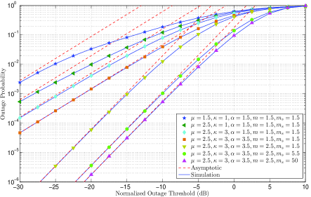
The OP is defined as the probability of falling the values of the output SNR below a predefined threshold value $\varphi$.

The OP, $P_{o}$, can be computed by [1, eq. (1.4)]

$\displaystyle P_{o}=F_{\gamma}(\varphi).$ (17)

where $F_{\gamma}(.)$ is provided in (6).

The asymptotic of the OP, $P^{\infty}_{o}$, can be analysed by (7), i.e., $P^{\infty}_{o}=F^{\infty}_{\gamma}(\varphi)$. Furthermore, the $P^{\infty}_{o}$ may be closely represented as $P^{\infty}_{o}\simeq\bar{\gamma}^{-G_{d}}$ whereby $G_{d}$ denotes the diversity gain that demonstrates the increasing in the slope of the OP versus $\bar{\gamma}$. Hence, plugging $\sigma_{j}$ of (16) in (7), one can notice that the values of the $G_{d}$ of the MGS and double shadowed $\alpha-\kappa-\mu$ are proportional to $\beta_{j}$ and $m$, respectively.

π’œΒ―=1βˆ’βˆ‘l=0uβˆ’1βˆ‘i=0l(l+uβˆ’1lβˆ’i)​2βˆ’(l+i+u)i!​(msβˆ’1)iβ€‹βˆ‘j=1KΟƒj​(ms)Ξ²j​Γ​(Ξ²j+i)​U​(Ξ²j+i;iβˆ’ms+1;msβˆ’12​΢j).Β―π’œ1superscriptsubscript𝑙0𝑒1superscriptsubscript𝑖0𝑙binomial𝑙𝑒1𝑙𝑖superscript2𝑙𝑖𝑒𝑖superscriptsubscriptπ‘šπ‘ 1𝑖superscriptsubscript𝑗1𝐾subscriptπœŽπ‘—subscriptsubscriptπ‘šπ‘ subscript𝛽𝑗Γsubscriptπ›½π‘—π‘–π‘ˆsubscript𝛽𝑗𝑖𝑖subscriptπ‘šπ‘ 1subscriptπ‘šπ‘ 12subscriptπœπ‘—\displaystyle\bar{\mathcal{A}}=1-\sum_{l=0}^{u-1}\sum_{i=0}^{l}{{l+u-1}\choose{l-i}}\frac{2^{-(l+i+u)}}{i!}(m_{s}-1)^{i}\sum_{j=1}^{K}\sigma_{j}(m_{s})_{\beta_{j}}\Gamma(\beta_{j}+i)U\bigg{(}\beta_{j}+i;i-m_{s}+1;\frac{m_{s}-1}{2\zeta_{j}}\bigg{)}. (34)

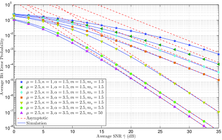
V-B Average Bit Error Probability

The ABEP can be evaluated by [1, eq. (9.11)]

$\displaystyle\bar{P}_{e}=\frac{1}{\pi}\int_{0}^{\frac{\pi}{2}}\mathcal{M}_{\gamma}\bigg{(}\frac{\rho}{\sin^{2}\phi}\bigg{)}d\phi.$ (18)

where $\rho=0.5$, $\rho=1$, and $\rho=0.715$ for coherent BFSK, BPSK, and BFSK with minimum correlation, respectively.

Substituting (8) into (18) and employing the identity [19, eq. (07.33.26.0004.01)], we have

PΒ―e=1π​Γ​(ms)β€‹βˆ‘j=1KΟƒjΞΆjΞ²jβ€‹βˆ«0Ο€2G1,22,1​[(msβˆ’1)​ρ΢j​sin2⁑ϕ|1βˆ’Ξ²j0,ms]​𝑑ϕ.subscript¯𝑃𝑒1πœ‹Ξ“subscriptπ‘šπ‘ superscriptsubscript𝑗1𝐾subscriptπœŽπ‘—subscriptsuperscript𝜁subscript𝛽𝑗𝑗superscriptsubscript0πœ‹2subscriptsuperscript𝐺2112delimited-[]conditionalsubscriptπ‘šπ‘ 1𝜌subscriptπœπ‘—superscript2italic-Ο•matrix1subscript𝛽𝑗0subscriptπ‘šπ‘ differential-ditalic-Ο•\displaystyle\bar{P}_{e}=\frac{1}{\pi\Gamma(m_{s})}\sum_{j=1}^{K}\frac{\sigma_{j}}{\zeta^{\beta_{j}}_{j}}\int_{0}^{\frac{\pi}{2}}G^{2,1}_{1,2}\bigg{[}\frac{(m_{s}-1)\rho}{\zeta_{j}\sin^{2}\phi}\bigg{|}\begin{matrix}1-\beta_{j}\\ 0,m_{s}\\ \end{matrix}\bigg{]}d\phi. (19)

By employing the definition of the Meijer’s $G$-function [19, eq. (07.34.02.0001.01)] and $t=\sin^{2}\phi$, (19) becomes

$\displaystyle\bar{P}_{e}$ =12​π​Γ​(ms)β€‹βˆ‘j=1KΟƒjΞΆjΞ²jβ€‹βˆ«011(1βˆ’t)​t​12​π​iβ€‹βˆ«β„’Ξ“β€‹(r)absent12πœ‹Ξ“subscriptπ‘šπ‘ superscriptsubscript𝑗1𝐾subscriptπœŽπ‘—subscriptsuperscript𝜁subscript𝛽𝑗𝑗superscriptsubscript0111𝑑𝑑12πœ‹π‘–subscriptβ„’Ξ“π‘Ÿ\displaystyle=\frac{1}{2\pi\Gamma(m_{s})}\sum_{j=1}^{K}\frac{\sigma_{j}}{\zeta^{\beta_{j}}_{j}}\int_{0}^{1}\frac{1}{\sqrt{(1-t)t}}\frac{1}{2\pi i}\int_{\mathcal{L}}\Gamma(r)
Γ​(ms+r)​Γ​(Ξ²jβˆ’r)​((msβˆ’1)​ρt​΢j)βˆ’r​d​r​d​t.Ξ“subscriptπ‘šπ‘ π‘ŸΞ“subscriptπ›½π‘—π‘Ÿsuperscriptsubscriptπ‘šπ‘ 1πœŒπ‘‘subscriptπœπ‘—π‘Ÿπ‘‘π‘Ÿπ‘‘π‘‘\displaystyle\Gamma(m_{s}+r)\Gamma(\beta_{j}-r)\bigg{(}\frac{(m_{s}-1)\rho}{t\zeta_{j}}\bigg{)}^{-r}drdt. (20)

where $i=\sqrt{-1}$ and $\mathcal{L}$ is the suitable contours in the $r$-plane from $\varrho-i\infty$ to $\varrho+i\infty$ with $\varrho$ is a constant value.

Changing the order of the integrations of (20) and then using [17, eq. (3.191.3)] for the linear integral, we obtain

PΒ―e=12​π​Γ​(ms)subscript¯𝑃𝑒12πœ‹Ξ“subscriptπ‘šπ‘ \displaystyle\bar{P}_{e}=\frac{1}{2\pi\Gamma(m_{s})} βˆ‘j=1KΟƒjΞΆjΞ²j​12​π​iβ€‹βˆ«β„’Ξ“β€‹(r)​Γ​(ms+r)​Γ​(Ξ²jβˆ’r)superscriptsubscript𝑗1𝐾subscriptπœŽπ‘—subscriptsuperscript𝜁subscript𝛽𝑗𝑗12πœ‹π‘–subscriptβ„’Ξ“π‘ŸΞ“subscriptπ‘šπ‘ π‘ŸΞ“subscriptπ›½π‘—π‘Ÿ\displaystyle\sum_{j=1}^{K}\frac{\sigma_{j}}{\zeta^{\beta_{j}}_{j}}\frac{1}{2\pi i}\int_{\mathcal{L}}\Gamma(r)\Gamma(m_{s}+r)\Gamma(\beta_{j}-r)
B​(r+0.5,0.5)​((msβˆ’1)​ρ΢j)βˆ’r​d​r.π΅π‘Ÿ0.50.5superscriptsubscriptπ‘šπ‘ 1𝜌subscriptπœπ‘—π‘Ÿπ‘‘π‘Ÿ\displaystyle B(r+0.5,0.5)\bigg{(}\frac{(m_{s}-1)\rho}{\zeta_{j}}\bigg{)}^{-r}dr. (21)

Recalling the properties [17, eq. (8.384.1)/ eq. (8.338.2)] and using [19, eq. (07.34.02.0001.01)], (21) is expressed as

PΒ―e=12​π​Γ​(ms)β€‹βˆ‘j=1KΟƒj​G2,22,1​[(msβˆ’1)​ρ΢j|1βˆ’Ξ²j,10,ms,0.5]ΞΆjΞ²j.subscript¯𝑃𝑒12πœ‹Ξ“subscriptπ‘šπ‘ superscriptsubscript𝑗1𝐾subscriptπœŽπ‘—subscriptsuperscript𝐺2122delimited-[]conditionalsubscriptπ‘šπ‘ 1𝜌subscriptπœπ‘—matrix1subscript𝛽𝑗10subscriptπ‘šπ‘ 0.5subscriptsuperscript𝜁subscript𝛽𝑗𝑗\displaystyle\bar{P}_{e}=\frac{1}{2\sqrt{\pi}\Gamma(m_{s})}\sum_{j=1}^{K}\frac{\sigma_{j}G^{2,1}_{2,2}\bigg{[}\frac{(m_{s}-1)\rho}{\zeta_{j}}\bigg{|}\begin{matrix}1-\beta_{j},1\\ 0,m_{s},0.5\\ \end{matrix}\bigg{]}}{\zeta^{\beta_{j}}_{j}}. (22)

The asymptotic of the ABEP at high $\bar{\gamma}$ regime, $\bar{P}^{\infty}_{e}$, can be deduced after inserting (9) in (18) and using $t=\sin^{2}\phi$ as

PΒ―eβˆžβ‰ƒ1Ο€β€‹βˆ‘j=1KΟƒj​(ms)Ξ²j​Γ​(Ξ²j)[(msβˆ’1)​ρ]Ξ²jβ€‹βˆ«01tΞ²j(1βˆ’t)​t​𝑑t.similar-to-or-equalssubscriptsuperscript¯𝑃𝑒1πœ‹superscriptsubscript𝑗1𝐾subscriptπœŽπ‘—subscriptsubscriptπ‘šπ‘ subscript𝛽𝑗Γsubscript𝛽𝑗superscriptdelimited-[]subscriptπ‘šπ‘ 1𝜌subscript𝛽𝑗superscriptsubscript01superscript𝑑subscript𝛽𝑗1𝑑𝑑differential-d𝑑\displaystyle\bar{P}^{\infty}_{e}\simeq\frac{1}{\pi}\sum_{j=1}^{K}\frac{\sigma_{j}(m_{s})_{\beta_{j}}\Gamma(\beta_{j})}{[(m_{s}-1)\rho]^{\beta_{j}}}\int_{0}^{1}\frac{t^{\beta_{j}}}{\sqrt{(1-t)t}}dt. (23)

The integration of (23) is recorded in [17, eq. (3.191.3)]. Thus, after some mathematical manipulations, this yields

PΒ―eβˆžβ‰ƒ12β€‹Ο€β€‹βˆ‘j=1KΟƒj​(ms)Ξ²j​Γ​(Ξ²j+0.5)Ξ²j​[(msβˆ’1)​ρ]Ξ²j.similar-to-or-equalssubscriptsuperscript¯𝑃𝑒12πœ‹superscriptsubscript𝑗1𝐾subscriptπœŽπ‘—subscriptsubscriptπ‘šπ‘ subscript𝛽𝑗Γsubscript𝛽𝑗0.5subscript𝛽𝑗superscriptdelimited-[]subscriptπ‘šπ‘ 1𝜌subscript𝛽𝑗\displaystyle\bar{P}^{\infty}_{e}\simeq\frac{1}{2\sqrt{\pi}}\sum_{j=1}^{K}\frac{\sigma_{j}(m_{s})_{\beta_{j}}\Gamma(\beta_{j}+0.5)}{\beta_{j}[(m_{s}-1)\rho]^{\beta_{j}}}. (24)

It is evident from (24) that the $G_{d}$ of the MGS model is proportional to $\beta_{j}$, i.e., $\bar{P}^{\infty}_{e}\simeq\bar{\gamma}^{-\beta_{j}}$. Hence, the $G_{d}$ for the double shadowed $\alpha-\kappa-\mu$ fading is proportional to $m$.

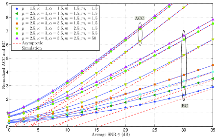
V-C Average Channel Capacity

According to Shannon’s theorem, the normalized ACC, $\bar{C}$, can be determined by [8, eq. (26)]

$$\bar{C}=\frac{1}{\ln(2)}\int_{0}^{\infty}\text{ln}(1+\gamma)f_{\gamma}(\gamma)d\gamma.$$ (25)

Plugging (4) in (25) and making use the identity [19, eq. (01.04.26.0002.01)] to write the natural logarithm in terms of the Meijer’s $G$-function, we obtain

$\displaystyle\bar{C}=$ (msβˆ’1)msln⁑(2)β€‹βˆ‘j=1KΟƒj​(ms)Ξ²jsuperscriptsubscriptπ‘šπ‘ 1subscriptπ‘šπ‘ 2superscriptsubscript𝑗1𝐾subscriptπœŽπ‘—subscriptsubscriptπ‘šπ‘ subscript𝛽𝑗\displaystyle\frac{(m_{s}-1)^{m_{s}}}{\ln(2)}\sum_{j=1}^{K}\sigma_{j}(m_{s})_{\beta_{j}}
$\displaystyle\times\int_{0}^{\infty}\frac{\gamma^{\beta_{j}-1}}{(m_{s}-1+\zeta_{j}\gamma)^{\beta_{j}+m_{s}}}G^{1,2}_{2,2}\bigg{[}\gamma\bigg{|}\begin{matrix}1,1\\ 1,0\\ \end{matrix}\bigg{]}d\gamma.$ (26)

Employing [17, eq. (7.811.5)], (26) can be expressed in exact closed-form as

CΒ―=1ln⁑(2)​Γ​(ms)β€‹βˆ‘j=1KΟƒjΞΆjΞ²j​G3,32,3​[msβˆ’1ΞΆj|1βˆ’Ξ²j,1,1ms,1,0].¯𝐢12Ξ“subscriptπ‘šπ‘ superscriptsubscript𝑗1𝐾subscriptπœŽπ‘—superscriptsubscriptπœπ‘—subscript𝛽𝑗subscriptsuperscript𝐺2333delimited-[]conditionalsubscriptπ‘šπ‘ 1subscriptπœπ‘—matrix1subscript𝛽𝑗11subscriptπ‘šπ‘ 10\displaystyle\bar{C}=\frac{1}{\ln(2)\Gamma(m_{s})}\sum_{j=1}^{K}\frac{\sigma_{j}}{\zeta_{j}^{\beta_{j}}}G^{2,3}_{3,3}\bigg{[}\frac{m_{s}-1}{\zeta_{j}}\bigg{|}\begin{matrix}1-\beta_{j},1,1\\ m_{s},1,0\\ \end{matrix}\bigg{]}. (27)

The asymptotic of the ACC for $\bar{\gamma}\rightarrow\infty$, $\bar{C}^{\infty}$, can be evaluated via [8, eq. (28)]

$\displaystyle\bar{C}^{\infty}\simeq\frac{1}{\ln(2)}\frac{\partial}{\partial n}\mathbb{E}[\gamma^{n}]\bigg{|}_{n=0}.$ (28)

Substituting (10) into (28), computing the partial derivative, and setting $n=0$, $\bar{C}^{\infty}$ over MGS model is deduced as

CΒ―βˆžβ‰ƒβˆ‘j=1KΟƒj​Γ​(Ξ²j)​[ln⁑(msβˆ’1ΞΆj)+Οˆβ€‹(Ξ²j)βˆ’Οˆβ€‹(ms)]ln⁑(2)​΢jΞ²j.similar-to-or-equalssuperscript¯𝐢superscriptsubscript𝑗1𝐾subscriptπœŽπ‘—Ξ“subscript𝛽𝑗delimited-[]subscriptπ‘šπ‘ 1subscriptπœπ‘—πœ“subscriptπ›½π‘—πœ“subscriptπ‘šπ‘ 2superscriptsubscriptπœπ‘—subscript𝛽𝑗\displaystyle\bar{C}^{\infty}\simeq\sum_{j=1}^{K}\frac{\sigma_{j}\Gamma(\beta_{j})\bigg{[}\ln\big{(}\frac{m_{s}-1}{\zeta_{j}}\big{)}+\psi(\beta_{j})-\psi(m_{s})\bigg{]}}{\ln(2)\zeta_{j}^{\beta_{j}}}. (29)

where $\psi(.)$ is the digamma function [17, eq. (8.360.1)].

V-D Effective Capacity

In Shannon’s theorem, the ACC has been measured under perfect quality of service (QoS). However, in the EC, the constraints of the QoS, such as, system delay, are taken into consideration [5].

The EC can be calculated by [15, eq. (4)]

$\displaystyle\mathcal{R}=-\frac{1}{A}\text{log}_{2}\bigg{\{}\int_{0}^{\infty}(1+\gamma)^{-A}f_{\gamma}(\gamma)d\gamma\bigg{\}}.$ (30)

where $A\triangleq\theta TB/\mathrm{ln}(2)$ with $\theta$, $T$, and $B$ denote the delay exponent, the time and the bandwidth of the channel.

Inserting (4) in (30) and employing [17, eq. (3.197.1)], the expression of the EC over MGS distribution is yielded as

$\displaystyle\mathcal{R}$ $\displaystyle=-\frac{1}{A}\text{log}_{2}\bigg{\{}\sum_{j=1}^{K}\frac{\sigma_{j}(m_{s})_{\beta_{j}}B(\beta_{j},m_{s}+A)}{(m_{s}-1)^{\beta_{j}}}$
$\displaystyle\times{{}_{2}F_{1}}\bigg{(}\beta_{j}+m_{s},\beta_{j};\beta_{j}+m_{s}+A;1-\frac{\zeta_{j}}{m_{s}-1}\bigg{)}\bigg{\}}.$ (31)

Plugging (5) in (30) and recalling [17, eq. (3.194.3)], the asymptotic of the EC at $\bar{\gamma}\rightarrow\infty$, $R^{\infty}$, is deduced as

Rβˆžβ‰ƒβˆ’1A​log2​{βˆ‘j=1KΟƒj​(ms)Ξ²j(msβˆ’1)Ξ²j​B​(Ξ²j,Aβˆ’Ξ²j)}.similar-to-or-equalssuperscript𝑅1𝐴subscriptlog2superscriptsubscript𝑗1𝐾subscriptπœŽπ‘—subscriptsubscriptπ‘šπ‘ subscript𝛽𝑗superscriptsubscriptπ‘šπ‘ 1subscript𝛽𝑗𝐡subscript𝛽𝑗𝐴subscript𝛽𝑗\displaystyle R^{\infty}\simeq-\frac{1}{A}\text{log}_{2}\bigg{\{}\sum_{j=1}^{K}\frac{\sigma_{j}(m_{s})_{\beta_{j}}}{(m_{s}-1)^{\beta_{j}}}B(\beta_{j},A-\beta_{j})\bigg{\}}. (32)

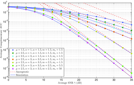
V-E Average AUC of Energy Detection

The AUC is a single figure of merit that is suggested as an alternative performance measure to the ROC curve [14].

The average AUC, $\bar{\mathcal{A}}$, can be computed by [20, eq. (20)/ eq. (21)]

$\displaystyle\bar{\mathcal{A}}$ $\displaystyle=1-\sum_{l=0}^{u-1}\sum_{i=0}^{l}\frac{{{l+u-1}\choose{l-i}}}{2^{l+i+u}i!}\int_{0}^{\infty}\gamma^{i}e^{-\frac{\gamma}{2}}f_{\gamma}(\gamma)d\gamma.$ (33)

where ${a\choose b}=\frac{a!}{b!(a-b)!}$ is the binomial coefficient.

Plugging (6) in (33) and utilizing [18, eq. (13.2.5)], $\bar{\mathcal{A}}$ is yielded as in (34) given at the top of this page.

The average AUC at high $\bar{\gamma}$ value, $\bar{\mathcal{A}}^{\infty}$, can be evaluated after inserting (5) in (33) and invoking [17, eq. (3.381.4)] as

π’œΒ―βˆžβ‰ƒ1βˆ’βˆ‘l=0uβˆ’1βˆ‘i=0lβˆ‘j=1KΟƒj​(ms)Ξ²j​(l+uβˆ’1lβˆ’i)​Γ​(Ξ²j+i)2l+uβˆ’Ξ²j​(msβˆ’1)Ξ²j​i!.similar-to-or-equalssuperscriptΒ―π’œ1superscriptsubscript𝑙0𝑒1superscriptsubscript𝑖0𝑙superscriptsubscript𝑗1𝐾subscriptπœŽπ‘—subscriptsubscriptπ‘šπ‘ subscript𝛽𝑗binomial𝑙𝑒1𝑙𝑖Γsubscript𝛽𝑗𝑖superscript2𝑙𝑒subscript𝛽𝑗superscriptsubscriptπ‘šπ‘ 1subscript𝛽𝑗𝑖\displaystyle\bar{\mathcal{A}}^{\infty}\simeq 1-\sum_{l=0}^{u-1}\sum_{i=0}^{l}\sum_{j=1}^{K}\frac{\sigma_{j}(m_{s})_{\beta_{j}}{{l+u-1}\choose{l-i}}\Gamma(\beta_{j}+i)}{2^{l+u-\beta_{j}}(m_{s}-1)^{\beta_{j}}i!}. (35)

VI Analytical and Simulation Results

In this section, the numerical and the asymptotic results of the derived performance measures are presented for different scenarios. To achieve MSE $\leq 10^{-5}$, we have used $K=15$.

Figs. 1-4 demonstrate the OP for $\varphi=5$ dB, the ABEP for BPSK modulation, the comparison between the normalized ACC and the EC for $A=3.5$, and the average complementary of AUC (CAUC), $1-\bar{\mathcal{A}}$, for $u=3$ versus $\bar{\gamma}$, respectively. Three cases for the shadowing index mssubscriptπ‘šπ‘ m_{s}, namely, heavy (ms=1.5subscriptπ‘šπ‘ 1.5m_{s}=1.5), moderate (ms=5.5subscriptπ‘šπ‘ 5.5m_{s}=5.5), and light (ms=50subscriptπ‘šπ‘ 50m_{s}=50) are analyzed.

From the provided results, it can be observed that the performance becomes better when $\alpha$, $\kappa$ and/or $\mu$ increase. This is because the high values of $\alpha$, $\kappa$, and $\mu$ indicate that the system tends to be linear, the total power of the dominant components is less than that of the scattered waves and large number of multipath clusters arrive at the receiver, respectively. Additionally, the increasing in $m$ and/or mssubscriptπ‘šπ‘ m_{s} means the impacts of the first and/or the second shadowing on the received signal are low. However, $m$ has the high effect on the performance when $\bar{\gamma}\rightarrow\infty$ due to improving in the $G_{d}$.

In Fig. 3, one can note that the ACC is higher than the EC for the same scenario. This refers to the impact of the system delay on the EC whereas its ignored in the ACC. Moreover, the EC is related to the average AUC via $u$ [20]. This relationship explains how the low quality of the received signal by the unlicensed user would reduce the detectability of the ED.

In all figures, a perfect agreement between the exact and the simulation results as well as the asymptotic at high $\bar{\gamma}$ can be noticed which proves the validation of our expressions.

Refer to caption
Figure 1: OP versus normalized outage threshold for $\varphi=5$ dB.
Refer to caption
Figure 2: ABEP for BPSK versus average SNR.
Refer to caption
Figure 3: Normalized ACC and EC with $A=3.5$ versus average SNR.
Refer to caption
Figure 4: Complementary AUC for $u=3$ versus average SNR.

VII Conclusions

In this paper, a MGS distribution was proposed as highly accurate approximate unified representation where the shadowing impact was assumed to be an inverse Nakagami-$m$ RV. This distribution was then applied to the double shadowed $\alpha-\kappa-\mu$ fading channel. The exact and the asymptotic expressions of the OP, the ABEP, the ACC, and the ER of the wireless communications systems and the average AUC of ED over a MGS model were derived. The results for different values of the fading parameters were presented. The expressions of this work can be employed for many fading conditions, such as, $\alpha-\kappa-\mathcal{F}$ fading with $m\rightarrow\infty$.

References

  • [1] M. K. Simon and M.-S. Alouini, Digital Communications over Fading Channels. New York: Wiley, 2005.
  • [2] M. D. Yacoub, $``$The $\kappa-\mu$ distribution and the $\eta-\mu$ distribution,$"$ IEEE Antennas Propag. Mag., vol. 49, no. 1, pp. 68-81, Feb. 2007.
  • [3] M. D. Yacoub, $``$The $\alpha-\mu$ distribution: a physical fading model for the Stacy distribution,$"$ IEEE Trans. Veh. Technol., vol. 56, no. 1, pp. 27-34, Jan. 2007.
  • [4] J. Zhang et al. , $``$Performance analysis of digital communication systems over composite $\eta-\mu$/gamma fading channels,$"$ IEEE Trans. Veh. Technol., vol. 61, no. 7, pp. 3114-3124, Sep. 2012.
  • [5] S. K. Yoo et al., $``$Effective capacity analysis over generalized composite fading channels$"$ IEEE Access, vol. 8, pp. 123756-123764, Jul. 2020.
  • [6] J. F. Paris, $``$Statistical characterization of $\kappa-\mu$ shadowed fading,$"$ IEEE Trans. Veh. Technol., vol. 63, no. 2, pp. 518-526, Feb. 2014.
  • [7] P. C. Sofotasios and S. Freear, $``$The $\alpha-\kappa-\mu$/gamma distribution: A generalized non-linear multipath/shadowing fading model,$"$ in Proc. IEEE INDICON, India, Dec. 2011, pp. 1-6.
  • [8] S. K. Yoo et al., $``$A comprehensive analysis of the achievable channel capacity in $\mathcal{F}$ composite fading channels,$"$ IEEE Access, vol. 7, pp. 34078-34094, Feb. 2019.
  • [9] O. S. Badarneh, $``$The $\alpha-\mathcal{F}$ composite fading distribution: Statistical characterization and applications,$"$ IEEE Trans. Veh. Technol., vol. 69, no. 8, pp. 8097-8106, May 2020.
  • [10] β€”β€”, $``$The $\alpha-\eta-\mathcal{F}$ and $\alpha-\kappa-\mathcal{F}$ composite fading distributions,$"$ IEEE Commun. Lett., vol. 24, no. 9, pp. 1924-1928, May 2020.
  • [11] O. S. Badarneh et al., $``$The $\alpha-\eta-\kappa-\mathcal{F}$ composite fading distribution,$"$ IEEE Wireless Commun. Lett., pp. 1-1, Aug. 2020.
  • [12] N. Simmons, et al., $``$On shadowing the $\kappa-\mu$ fading model,$"$ IEEE Access, vol. 8, pp. 120513-120536, Jun. 2020.
  • [13] S. Atapattu, C. Tellambura, and H. Jiang, $``$A mixture gamma distribution to model the SNR of wireless channels,$"$ IEEE Trans. Wireless Commun., vol. 10, no. 12, pp. 4193-4203, Dec. 2011.
  • [14] H. Al-Hmood and H. S. Al-Raweshidy, $``$Unified modeling of composite $\kappa-\mu$/gamma, $\eta-\mu$/gamma, and $\alpha-\mu$/gamma fading channels using a mixture gamma distribution with applications to energy detection,$"$ IEEE Antennas Wireless Propag. Lett., vol. 16, pp. 104-108, Apr. 2017.
  • [15] H. Al-Hmood and H. S. Al-Raweshidy, $``$Unified approaches based effective capacity analysis over composite $\alpha-\eta-\mu$/gamma fading channels,$"$ Electronics Lett., vol. 54, no. 13, pp. 852-853, Jun. 2018.
  • [16] H. Al-Hmood and H. S. Al-Raweshidy, $``$Unified analysis of channel capacity under different adaptive transmission policies,$"$ Electronics Lett., vol. 56, no. 2, pp. 87-89, Jan. 2020.
  • [17] I. S. Gradshteyn, and I. M. Ryzhik, Table of Integrals, Series and Products, 7th edition. Academic Press Inc., 2007.
  • [18] M. Abramowitz and I. A. Stegun, Handbook of Mathematical Functions: With Formulas, Graphs, and Mathematical Tables. New York, NY, USA: Dover, 1965.
  • [19] Wolfram Research, Inc., 2020, [Online]. Available: http://functions.wolfram.com/id. Accessed on: Oct. 2020.
  • [20] H. Al-Hmood, and H. S. Al-Raweshidy, $``$On the effective rate and energy detection based spectrum sensing over $\alpha-\eta-\kappa-\mu$ fading channels,$"$ IEEE Trans. Veh. Technol., vol. 69, no. 8, pp. 9112-9116, Aug. 2020.